1. Introduction
The M7.1 Hector Mine earthquake on October 16, 1999, was preceded by a very strong foreshock, which the whole seismological world experienced after a heated discussion in the pages of the Nature journal, started on 25 February 1999, by Robert Geller of the University of Tokyo [
1]. The discussion was based on his earlier critical review of 1997, which argued that short-term earthquake forecasting is impossible [
2]. At almost the same time, a paper was published that showed that electromagnetic coupling is possible between processes in the earth’s crust and in the ionosphere, where the Global Electric Circuit’s atmospheric electric field (GEC) plays the main role [
3]. Following this idea, studies were carried out during the past 20 years, which demonstrated that the earth’s crust affects the physical processes in the upper geospheric shells in seismically active regions. A physical model of the interaction of geospheres was created, called the Lithosphere–Atmosphere–Ionosphere Coupling (LAIC) model. The last two versions of the model were published in 2015 and 2018 [
4,
5], where the model’s genesis can be found in the References list since 2000. The last work in which the seismic-ionospheric couplings mechanism is considered exclusively was published in 2019 [
6]. It is essential that a physical substantiation has been obtained to initiate specific variations in the atmosphere and ionosphere, which appear several days before the earthquake, having the potential to be used as earthquake precursors. But in this way, it is necessary to develop technology for recognizing these variations against the background of the high variability of the ionosphere (if we are talking about ionospheric precursors).
The very concept of the LAIC model was well received, but as soon as the first publications appeared, allowing the precursors’ identification [
7,
8] which opened the way to a short-term forecast, they immediately seemed to express the opposite opinion, denying such a possibility [
9,
10]. The Hector Mine earthquake became a kind of stumbling block in the struggle for the ionospheric precursors. As soon as [
11] showed, using the global ionospheric maps (GIM) mapping technology, that the ionospheric anomalies before the Hector Mine earthquake were of a local nature, the publication was immediately followed by [
12], denying the apparent picture of the presence of such anomalies. Unfortunately, the authors mentioned above expressed an opinion supporting the nonexistence of physical precursors. In many of their papers, the results of pre-earthquake signals have been reviewed and disproved as nonexisting physical phenomena associated with earthquakes of any origin, regardless of geomagnetic, electromagnetic, or ionospheric ones.
In this study, we carefully analyzed the arguments of critics of ionospheric precursors, describing the Hector Mine case. In that case, they are all based on playing with the amplitude variations of the Total Electron Content (GPS TEC) and attempt to explain all the observed anomalies by high geomagnetic activity in October 1999. At the same time, they lose sight of the fact that the physics of the effect on the ionosphere of the earthquake preparation process is fundamentally different from the mechanism of the effect on the ionosphere of geomagnetic storms, which we pointed out back in 2003 [
13]. The spatial locality and dependence of the ionospheric precursors on local time, not to mention more subtle things associated with a change in the vertical profile of electron concentration, make it possible to unambiguously identify the ionospheric precursors, even in the most challenging cases of ionospheric disturbance. In this case, variations in the electron concentration before different earthquakes are not chaotic but have the property of close similarity. One example is the overnight positive variation in electron concentration [
14], which makes the process of identifying the precursor deterministic [
15]. Multiparameter analysis involving various types of precursors [
16] and the use of various technologies for monitoring the ionosphere (vertical sounding, GPS TEC, radio occultation technologies, ionospheric tomography, etc.) make it possible to recognize ionospheric precursors with high accuracy. We call this approach “cognitive identification” [
17].
The last major California earthquake, the M7.1 Ridgecrest earthquake on July 5, 2019, provides an excellent opportunity to demonstrate the benefits of cognitive identification, as well as to explore the uniqueness and similarity of two earthquakes of the same magnitude that occurred in the same region but under different solar and geomagnetic conditions with an interval of 20 years.
In this work, we present results from analyzing the ionosphere and atmosphere for two strong earthquakes of the same magnitude, M7.1 in 1999 at Hector Mine and the Ridgecrest earthquakes of 4 July 2019, which occurred in the same region (North-East from Los Angeles, California). To perform this work, we analyzed data from a local network of GPS receivers in California, Global Ionospheric Maps provided by NASA in IONEX format, and ground-based vertical sounding ionosonde. The preview of the structure as follows:
Section 1 and
Section 2 summarize the studies of two earthquakes;
Section 3 previews the geomagnetic conditions during the time of both events,
Section 4 and
Section 5 describe GPS TEC analysis and Ionosphere Mapping,
Section 6 focuses on achieving results, and
Section 7 reports the final remarks of the work.
2. Seismo-Tectonic Conditions of the Hector-Mine and Ridgecrest Earthquakes
Both events happened not far from one another (~160 km) in South-eastern California along the line following the lineaments of main tectonic faults direction from South-East (Hector Mine) to North-West (Ridgecrest). Both events have a similar mechanism—right-lateral strike-slip along the local faults (Lavic Lake fault for Hector Mine and Airport Lake fault for Ridgecrest). For both events, the foreshocks were registered, but here we can mark the difference. In the case of the Hector Mine earthquake, 50 weak foreshocks with magnitude 0.4 < M < 3.7 were registered in the 20 h leading up to the main event [
18]. The M7.1 Ridgecrest event was preceded by a strong M6.4 foreshock, followed by a 34-hour-long earthquake sequence that led up to the M 7.1 event [
19]. The sequence included five moderate earthquakes 4.5 < M < 5.4. The M6.4 foreshock was preceded by the M4.0 event ~31 min before, and was followed by smaller events. We will not concentrate on the aftershocks of these events because our paper is devoted to their precursors, and we look for information that may help their detection.
Our previous investigations [
5] demonstrated that the foreshock period is accompanied by the short-term precursors of different origins, including the ionospheric ones. One of the foreshock period’s seismic indicators is the drop of the
b-value (
b–coefficient in the Gutenberg-Richter relationship) before the mainshock [
20]. Schorlemmer and Wiemer [
21] concluded that “
b values could be used for accurately predicting rupture areas: although the timing of earthquakes remains unpredictable”. We examined the literature on the possible variations of the
b-value before the Hector Mine and Ridgecrest earthquakes [
19,
22]. From these, we can conclude that the b-value drop was registered before the mainshock in both cases. This fact gives us a hope that the short-term precursors were present and could be analyzed from the point of view of their similarity, not excluding the difference in some individual parameters. Our main emphasis will be put on ionospheric precursors, which were registered by the local network of GPS receivers in California, Global Ionospheric Maps provided by NASA in IONEX format, and ground-based vertical sounding ionosonde at Point Arguello.
3. The Principles of Ionospheric Precursors Detection
Our approach is based on the following main principle: we look for not a kind of anomaly detected by statistical processing but a result of developing the physical process responsible for the ionospheric precursor’s generation [
14]. To give confidence, we use the set of techniques for multiparameter data processing developed and tested as practical applications for a large set of major earthquakes worldwide [
17,
23], which we name “cognitive recognition”.
The ionospheric precursors should have the following phenomenological properties [
13]:
It should be local in space and should indicate by its position the location of the impending earthquake epicenter (the latter feature is checked after the event).
It should have clear dependence on the local time (most often in the middle latitudes, we observe the positive night-time variation of the electron concentration in the ionosphere).
The precursor appears within the time interval 10–1 days before the mainshock.
The size of the large-scale irregularity in the ionosphere in its maximum phase of temporal development depends on the magnitude of the impending earthquake.
In case of availability of the satellite data (topside sounding, local plasma parameters), the precursors could be identified by the variation of the height scale, electron temperature variations, and variations of the main ion’s composition.
Special visualization procedures called the “precursor mask” [
14] permit identifying the ionospheric precursors even in conditions of strong geomagnetic disturbances.
In the case of ground-based vertical sounding data availability, specific features registered on ionograms during the precursory period give additional information on the earthquake approaching [
24].
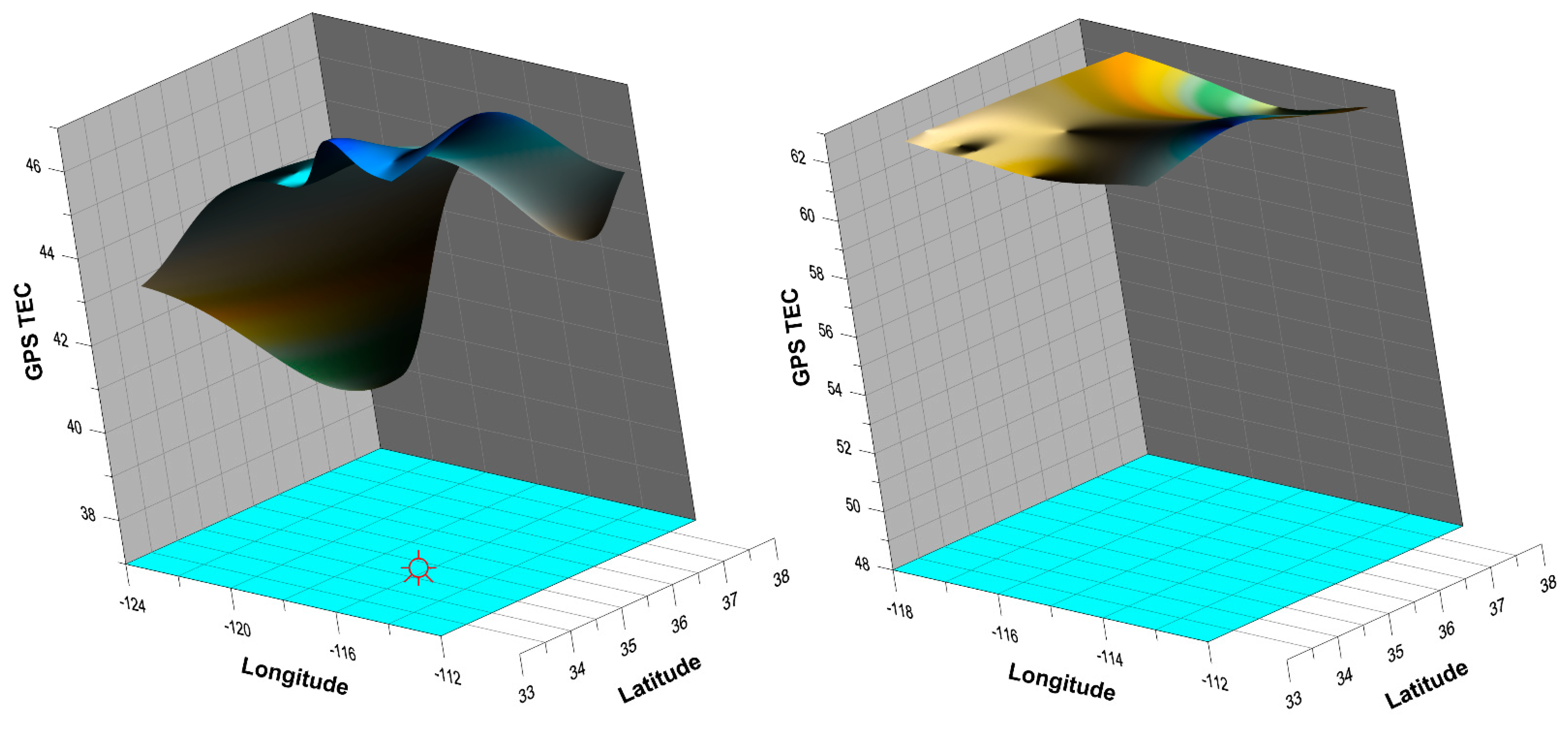
The difference between the ionospheric variations over the earthquake preparation zone during precursory periods and in conditions of geomagnetic disturbance should be discussed. The system of electromagnetic fields and currents during a geomagnetic storm has a global character, and on the scales of a few thousand kilometers (until the local time effects will be essential due to longitude difference), the ionosphere will react identically as if it is a solid plane. Before earthquakes, the gas emission (bringing radon to the surface) has a mosaic character. The strain and stress are distributed irregularly following the complex structure of the area’s tectonic faults and block structure. The electric fields and variations of air conductivity also have an irregular and mosaic character, which demonstrates the appearance of several sources of acoustic gravity waves moving in different directions [
25] and initiating the traveling ionospheric disturbances. It will stimulate an event which we call the Local Ionosphere Variability [
23]. Just for the case of the Hector Mine earthquake (when the ionosphere was magnetically disturbed), we plotted two spatial TEC distributions during the precursory period (
Figure 1, left panel) and geomagnetic storm (
Figure 1, right panel). One can see the drastic difference in the spread of TEC values: in the left panel during precursory period s = 4.08, while during a geomagnetic storm in the right panel s = 1.48.
Using the principles mentioned above, it is possible to unambiguously identify the ionospheric precursors, which we intend to demonstrate in the following paragraphs.
4. Solar and Geomagnetic Conditions around the Time of the Hector Mine Earthquake on 16 October 1999 and Ridgecrest Earthquake on 5 July 2019
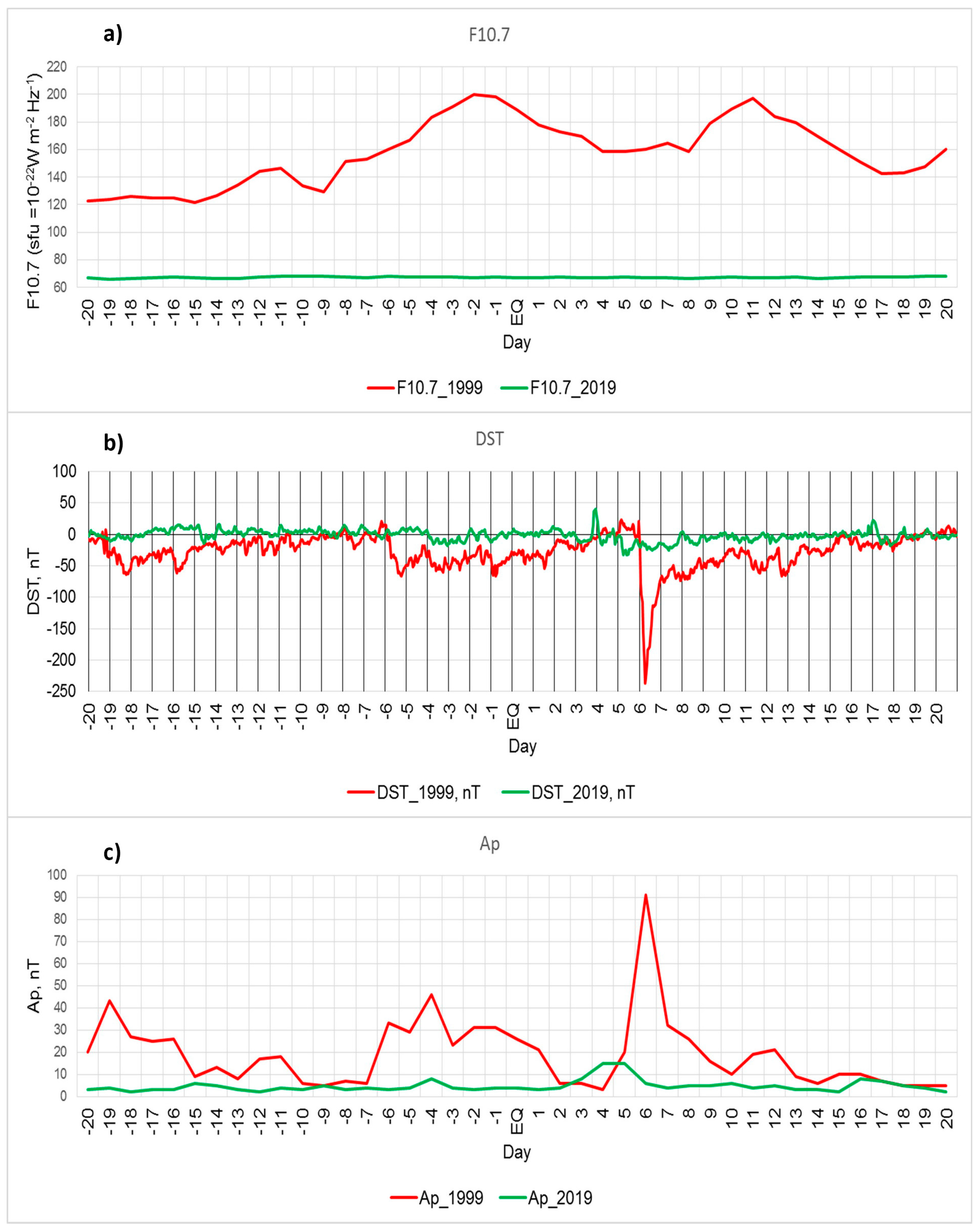
As mentioned earlier, the earthquakes happened in quite different geophysical conditions: the Hector Mine earthquake took place in the middle of the rising phase of the 23rd solar cycle, while the Ridgecrest earthquake happened close to the solar minimum during the falling phase of the 24th cycle. Besides, just during the Hector Mine earthquake, the values of F10.7 reached the magnitude equal to values of the solar maximum. In turn, the 24th solar cycle was extremely weak compared to the two previous cycles, which led to the fact that the solar activity during the Ridgecrest earthquake was nearly three times weaker than during the Hector Mine earthquake (see the top panel of
Figure 2). Consequently, the absolute values of TEC for the period of the Hector Mine earthquake are more than three times larger than values for the Ridgecrest earthquake period (see
Figure 3) regardless of the Ridgecrest earthquake being close to the summer solstice. At the same time, the Hector Mine earthquake was close to the fall equinox. We can see quite strong variations of the Hector Mine case’s solar activity during the observation period (value of 10.7 index changes from 120 on day -15 till 200 on days -2, -1). The maximum TEC values’ envelope follows the variations of the F10.7 index, except for the geomagnetic storm period on day 6 (DOY 295). The most reliable indicator of the geomagnetic storms is the global equatorial geomagnetic index Dst presented in
Figure 2b). For the Hector Mine period (red curve), we see that the whole period was strongly disturbed, with two small disturbances (days -18 and -6) and with a powerful geomagnetic storm, almost −250 nT (day 6). If identifying the strong magnetic storm effect in the ionosphere is not a problem, we should be cautious during the small disturbances to not mix effects in the ionosphere from these disturbances with ionospheric precursors, requiring additional identification tools.
Figure 2 shows the drastic difference in solar and geomagnetic activity for time intervals around the time of the earthquakes considered. The green lines corresponding to the Ridgecrest earthquake demonstrate extremely quiet conditions that are difficult to comment on except the small negligible disturbances on day four seen in Dst’s small positive peak. A small increase of Ap to 10 nT corresponds to quiet geomagnetic conditions.
5. GPS TEC Analysis
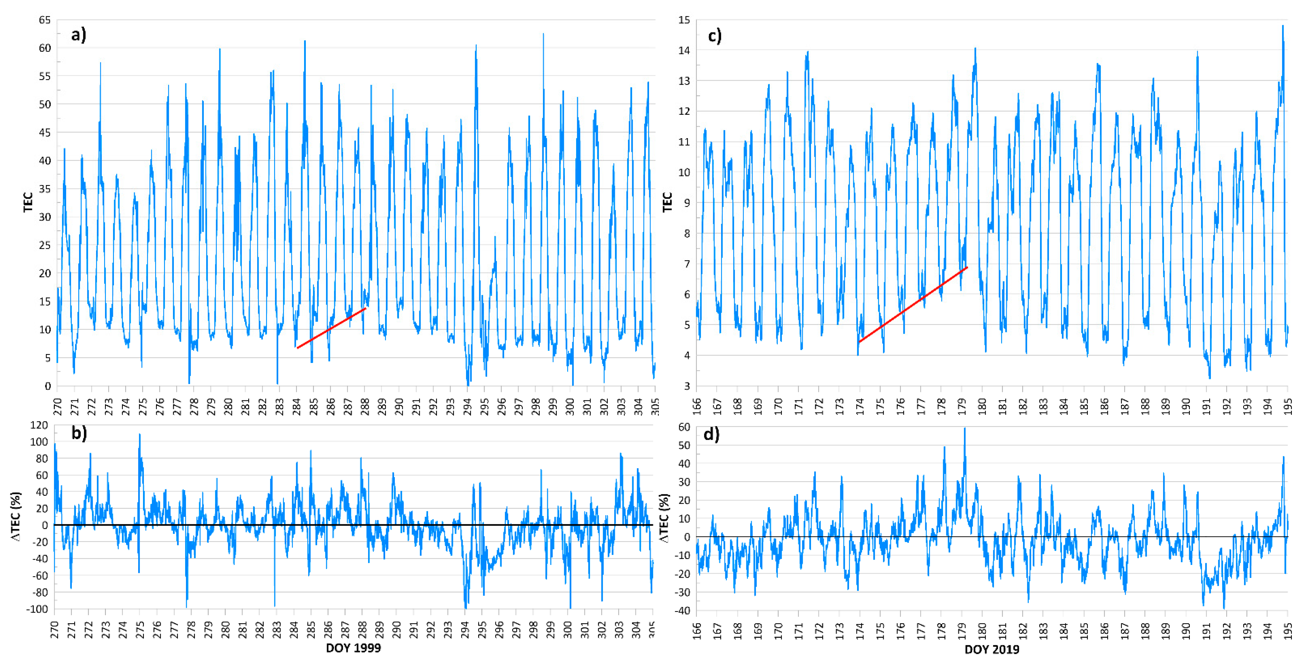
In
Figure 3a,c are presented the time series of the GPS TEC for the stations closest to the earthquake epicenter: (a)—station
gol2 the case of the Hector Mine earthquake; (c)—station
ramt for the Case of Ridgecrest earthquake. To see more in detail the TEC variability, the residual ⊗TEC is presented in a percentage format. Since the absolute TEC values at night can be an order of magnitude lower than the daytime values (which is quite natural), many authors neglect the small nighttime deviations in absolute values and come to incorrect conclusions regarding the presence or absence of precursors. In contrast, the primary game in the scene of precursors generation is played out at night. Conversely, the use of ⊗TEC as a percentage makes it possible to filter out the daily TEC changes associated with variations in the level of ultraviolet radiation from the sun that mainly forms the ionosphere.
Looking at the TEC variations and their residuals for both cases, it is challenging to say whether we see any variation that we can interpret as a precursor. We can see that the only major feature is the effect of the magnetic storm on 22 October (DOY295) of 1999. Moreover, instead of applying the statistical methods, at this point, we start the process of cognitive recognition. As it was demonstrated in [
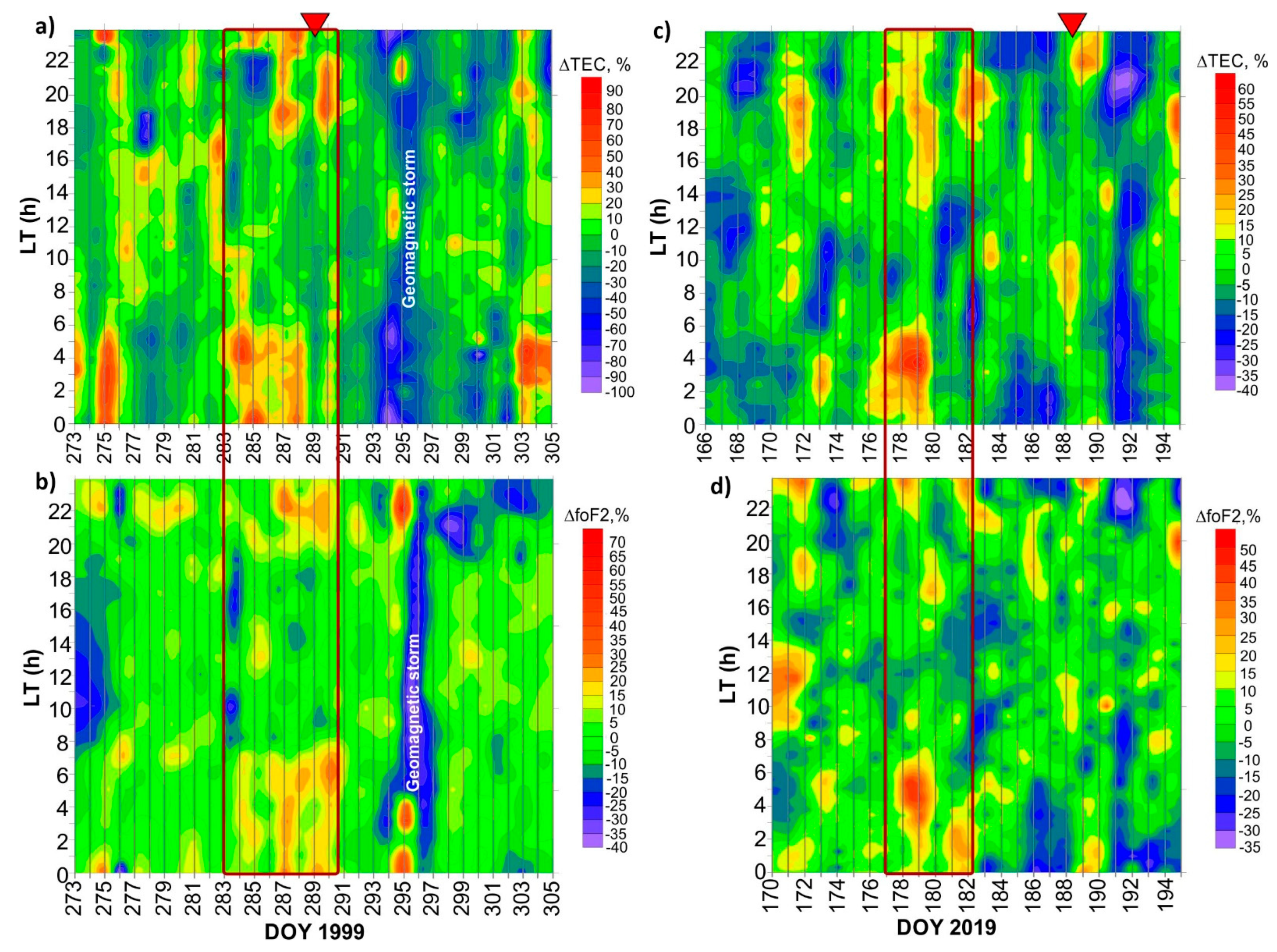
14], the precursor should look like the positive night-time deviation a few days before the earthquake, which could be revealed in the precursor mask shown in
Figure 4. We transformed color tones to express the ⊗TEC graphs shown in the bottom panel of
Figure 3 into two-dimensional distribution along axes of DOY as X and LT as Y. ⊗TEC (%) is expressed by color tones
In addition to the vertical TEC data we present in
Figure 4, the vertical sounding data from Point Arguello ionosonde in the same format (only instead of ΔTEC the ΔfoF2 is shown) provides insights. For the Hector Mine case, we see the positive night-time deviations of TEC and foF2 on days 284–289, and for the Ridgecrest earthquake, the positive variations during the night-time were registered on days 177–180. The only difference we can mark is the leading time of the precursor. If in 1999 the precursor was generated just a few days before the mainshock, in 2019 it appeared earlier; six days before the mainshock M7.1 and five days before the strongest foreshock M6.4. We will discuss this difference later, and here it is necessary to explain why the ionosonde data in 2019 are so messy. This is because of the automatic scaling. In 1999 the ionograms were processed manually. In 2019, the automatic scaling demonstrated the ragging lines instead of quasi-sinusoidal variations of the critical frequency in 1999, which is reflected on residuals. Just recently, a joined analysis of several types of physical precursors (lithosphere, atmosphere, and ionosphere) associated with the 2019 Ridgecrest earthquake was studied [
26]. The Ridgecrest earthquake preparation phase probably activated a series of anomalous patterns in the lithosphere, atmosphere, and ionosphere. The range of lag-time varies between 9 years (lithosphere), 25–79 days (atmosphere), and 25–34 days (ionosphere). Data from Point Arguello ionosondes were analyzed, and the anomaly was revealed on June 2. Our analysis of the same data revealed another anomaly on June 29. There are no contradictions between both results. Instead of in opposite, the results identify the natural processes in the ionosphere revealed by different techniques.
De Santis et al.’s approach identified the medium-term ionospheric precursors of earthquakes from Point Arguello ionosondes, which is inside the zone of earthquake preparation. Similar approaches have been studied and assessed statistically before [
27,
28]. Our analysis considers the short-term type of seismo-ionospheric precursors concerning the earthquake’s final stage as a chaotic process [
29] (the last 10 days before the main shock) when the foreshock sequence is registered together with the b-value decrease [
30] and when the precursor “masks” were formed, representing the ionosphere’s last state before the seismic event. Ideally, both results compliment each other. The results represent the complex developed in the ionosphere during the time of the earthquake preparation phase according to the temporal evolution as a function of magnitude [
31] and spatial allocation concerning the earthquake preparation zone [
32].
Returning to the registered night-time positive deviation of electron concentration presented in
Figure 4, we still do not claim that suspicious variations are precursors. We continue to apply our techniques of identification. As is shown in
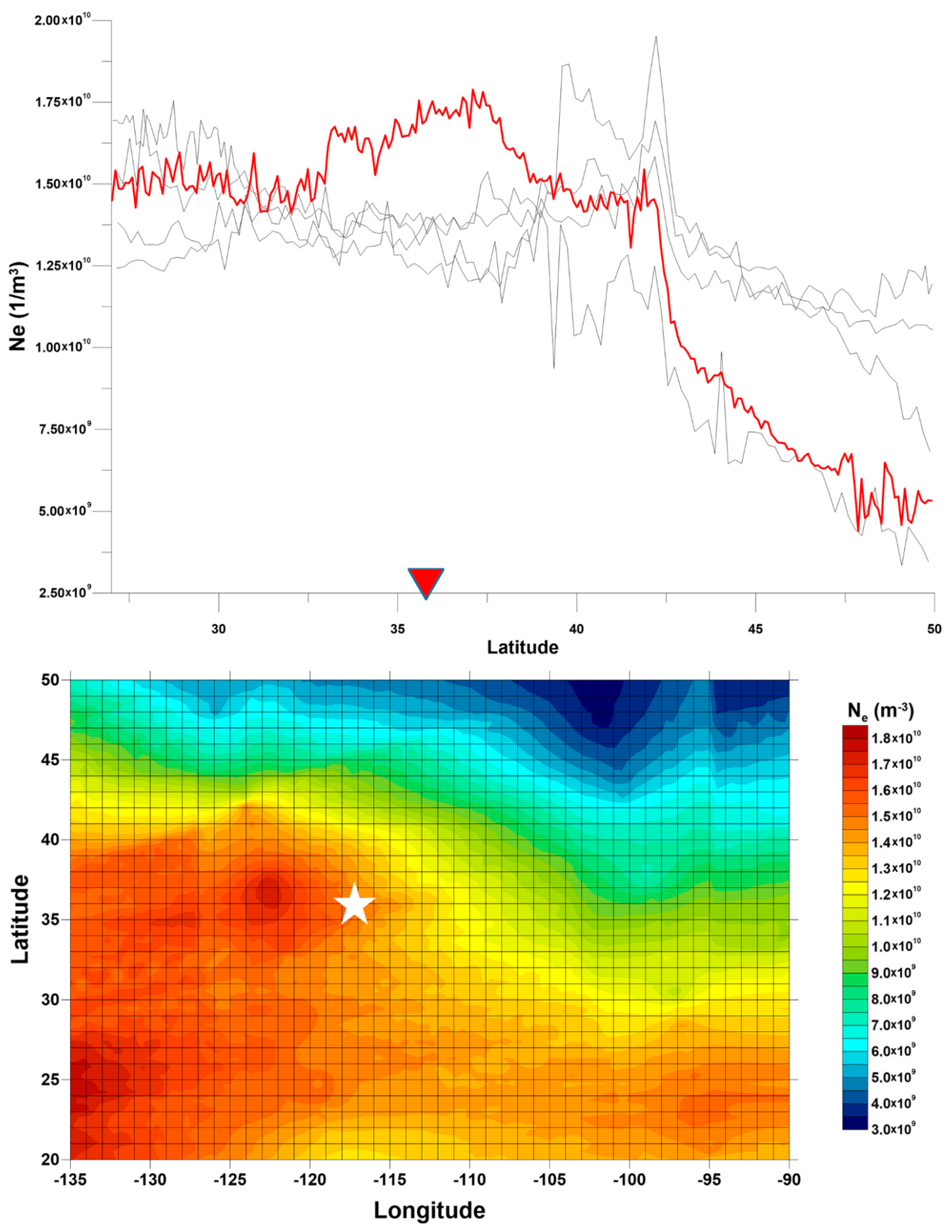
Figure 1, the spatial TEC variability in the vicinity of the epicenter during the precursory period was more extensive than in quiet and even magnetically stormy conditions. So, it is worth applying our spatial variability detection technique to calculate the local spatial variability coefficient. Nevertheless, now, instead of Max-Min analysis [
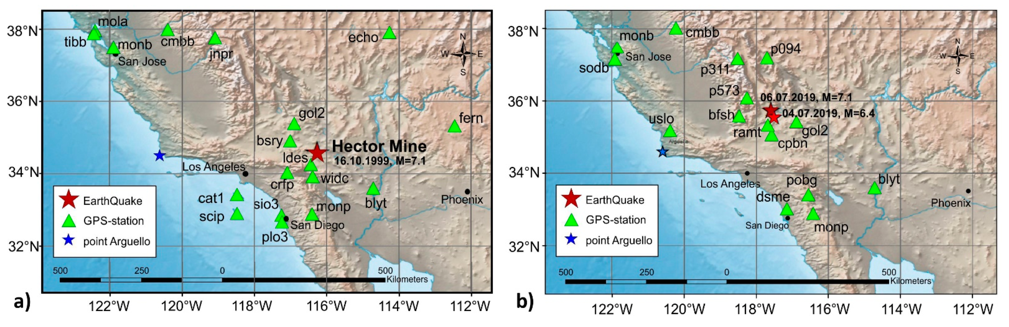
8], we will calculate root mean square deviation (RMSD) of TEC using the vertical series of TEC inside some regions (in our case, in South-East California). GPS receivers’ positions for the 1999 and 2019 cases are shown in
Figure 5.
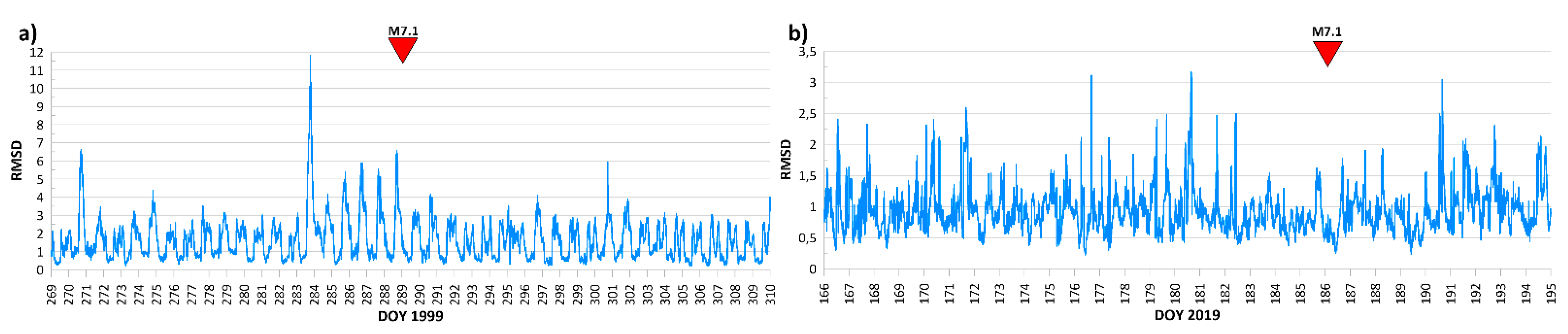
It should be noted that regardless of the fact that the positions of earthquake epicenters are marked by red stars in the figures, in the real analysis, we did not know their positions and used the set of receivers in a specific area of California. The time series of RMSD for the 1999 and 2019 cases are presented in
Figure 6.
As one can see, in both cases the time intervals of increased RMSD in TEC variations coincided with the time of the positive night-time variations of TEC, and critical frequency is demonstrated in
Figure 4. In 2019, the increased spatial variability was not critical because of the TEC values, which were three times lower compared with 1999. By this test, we take one step forward to determine these time intervals as precursory periods.
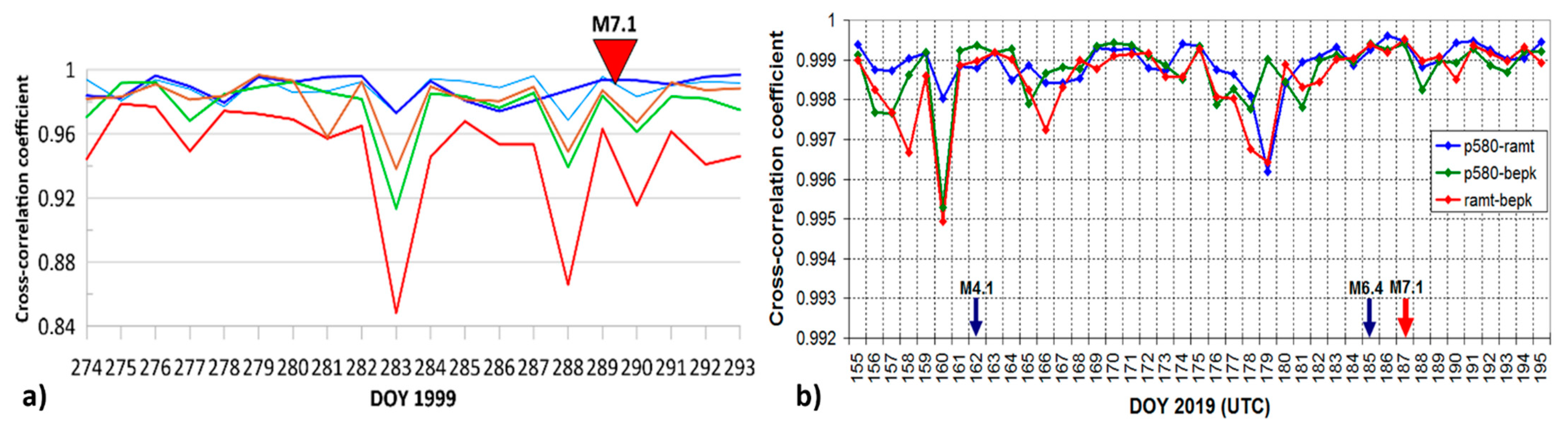
The last test dealing with time series was calculating the cross-correlation coefficient between pairs of stations according to the technology described in [
7]. The results are presented in
Figure 7.
In
Figure 7a (Hector Mine earthquake), we observe that the main minima of cross-correlation coefficients for different pairs of stations fall into the time interval indicated by the Index of spatial variability RMSD from 10 to 15 October, where 15 October is the day before the mainshock (
Figure 6). In the Ridgecrest earthquake (
Figure 7b) case, we observe an additional minimum appearing before the M4.1 foreshock having a place on 18 June 2019. The coherent minimum is observed inside the precursory interval for the Ridgecrest earthquake on 28 June (DOY 179) when the maximum deviations are observed in the precursor mask.
Summarizing the results of the multicomponent analysis of the GPS TEC monitoring over the areas of the M7.1 Hector Mine earthquake (1999) and Ridgecrest earthquake (2019), we can state that in both cases, the positive deviation in GPS TEC was registered during night-time. One can clearly see the positive trend of night-time TEC values marked by red lines on the time series in
Figure 3. These periods coincide with yellow and red spots in the morning and evening segments of precursors’ masks inside the blue rectangles both on the GPS and vertical sounding data (
Figure 4). We reveal the increased spatial variability over the area of earthquake preparation in the RMSD plots (
Figure 6) coinciding with the precursory periods observed at time series of TEC and foF2 on precursors’ masks. We observe a drop of cross-correlation coefficients value inside these intervals for both earthquakes (
Figure 7).
Still, we do not have the confidence that registered variations are precursors, except for the fact that they are similar to ionospheric variations recognized as a precursor for many other cases of ionospheric precursor studies. Still, we need proof of their regionality and have the instruments to estimate the earthquake magnitude. This is the problem we hope to resolve with ionospheric mapping technology.
6. Ionospheric Mapping
Determining the locality of the ionospheric anomaly detected needs application of the mapping procedure as an obligatory element of the precursor identification. If the precursor itself is detected by the GPS receiver/ionospheric station closest to the epicenter of the event, then its locality should be determined with the mapping procedure. Back in 2003, it was shown [
13] that the locality of an anomalous phenomenon in the ionosphere is the main necessary feature of an ionospheric precursor; therefore, the construction of the mask should be accompanied by the construction of differential maps of TEC over the earthquake preparation zone. In addition to confirming the precursor locality, differential maps also help to clarify the position of the earthquake epicenter and estimate its magnitude. In fact, the process of operational forecasting itself should begin with mapping; when a local anomaly is detected, it is necessary to construct a precursor mask based on the data of the receiver closest to the position of the maximum of the anomaly detected via mapping.
There are several options for mapping that exist today: the creation of maps with a local network of stationary GPS/GLONASS receivers, as was done for the case of the earthquake in Aquila in 2009 [
23], via vertical sounding from the satellite [
33]; high-orbit tomography [
34]; global ionospheric maps (GIMs) distributed by the International Global Navigation Satellite Systems (GNSS) Service (IGS) in the IONEX (IONosphere map EXchange) format [
35,
36]; and radio occultation sounding [
37].
Despite the low resolution of IONEX maps, they are currently the most suitable option for data availability and efficiency. The IGS data in IONEX format is a matrix with elements that are TEC values multiplied by 10. The matrix resolution is 2.5° in latitude and 5° in longitude. The TEC values are calculated by IGS every two hours (the transition to a time resolution of 1 h is currently underway). Differential maps of the global TEC—TECGIM, which represent the deviation of the current TEC
GIM values from the background TEC
GIMA, are calculated and constructed with the formula ΔTEC
GIM = (TEC
GIM–TEC
GIMA)/TEC
GIMA, where the moving average TEC values calculated for 15 previous days are used as background values for the same moment of the local time. Examples of differential maps for various earthquakes can be found in earlier works [
23].
Nevertheless, we should keep in mind that the local GPS receivers’ network in California is very dense, and the number of receivers included in the IGS service is far from complete: data of the small part of this network are included in the procedures of GIM maps constructing. From the other point of view, the local network practically has no receivers in the Pacific Ocean west from the California shore, while the GIM, using procedures of modeling and extrapolation, is able to provide the TEC values over the ocean as well.
In this regard, we decided to experimentalize by comparing the maps constructed with data from the local GPS receivers’ networks and from GIM.
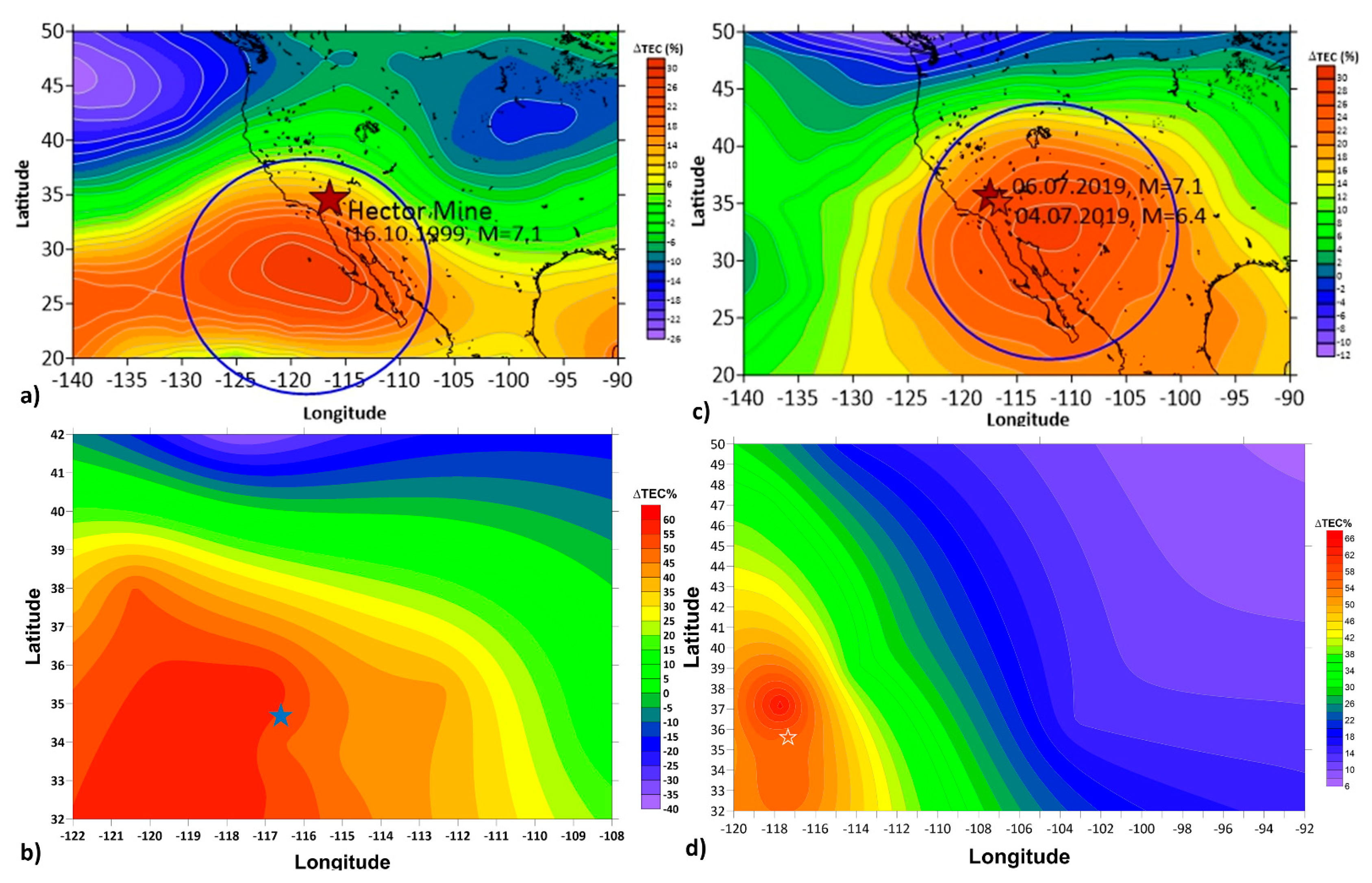
In
Figure 8a,b are the differential GIM and local GPS networks TEC maps built for DOY284 (11 October 1999) for 03:00 LT, and in
Figure 8c,d are the differential GIM and local GPS networks TEC maps built for DOY179 (28 June 2019) for 04:00 LT.
The difference in the local time selection for 1999 and 2019 cases is connected with the fact that in 1999 the IONEX index was calculated every two odd hours, but later IGS started to produce IONEX every two even hours. Nevertheless, the days for which the precursor maps were built were not chosen by chance; they were selected by the ionosphere itself, which in the set of maps appeared in a distribution where the isolated maximum revealed itself. Of course, we had in mind that we were looking for the night time distributions, but the expected distribution appeared on the day when the minimum of cross-correlation coefficient was registered and at the local time when the brightest spot at the precursor mask was revealed as well. This demonstrates the synergy of different factors of temporal behavior.
One can notice that the positions of maxima of the ⊗TEC do not coincide for GIM and the local GPS TEC distributions. Besides, these maxima do not coincide with the epicenter positions. According to our experience with ionospheric mapping using the different techniques, the GIM maps more adequately reflect the real situation, because the procedures of the data calibration and interpolation are more sophisticated than the simple Kriging procedure used for the local GPS TEC data. Local stations may have some bias, introducing false irregularities into the distribution.
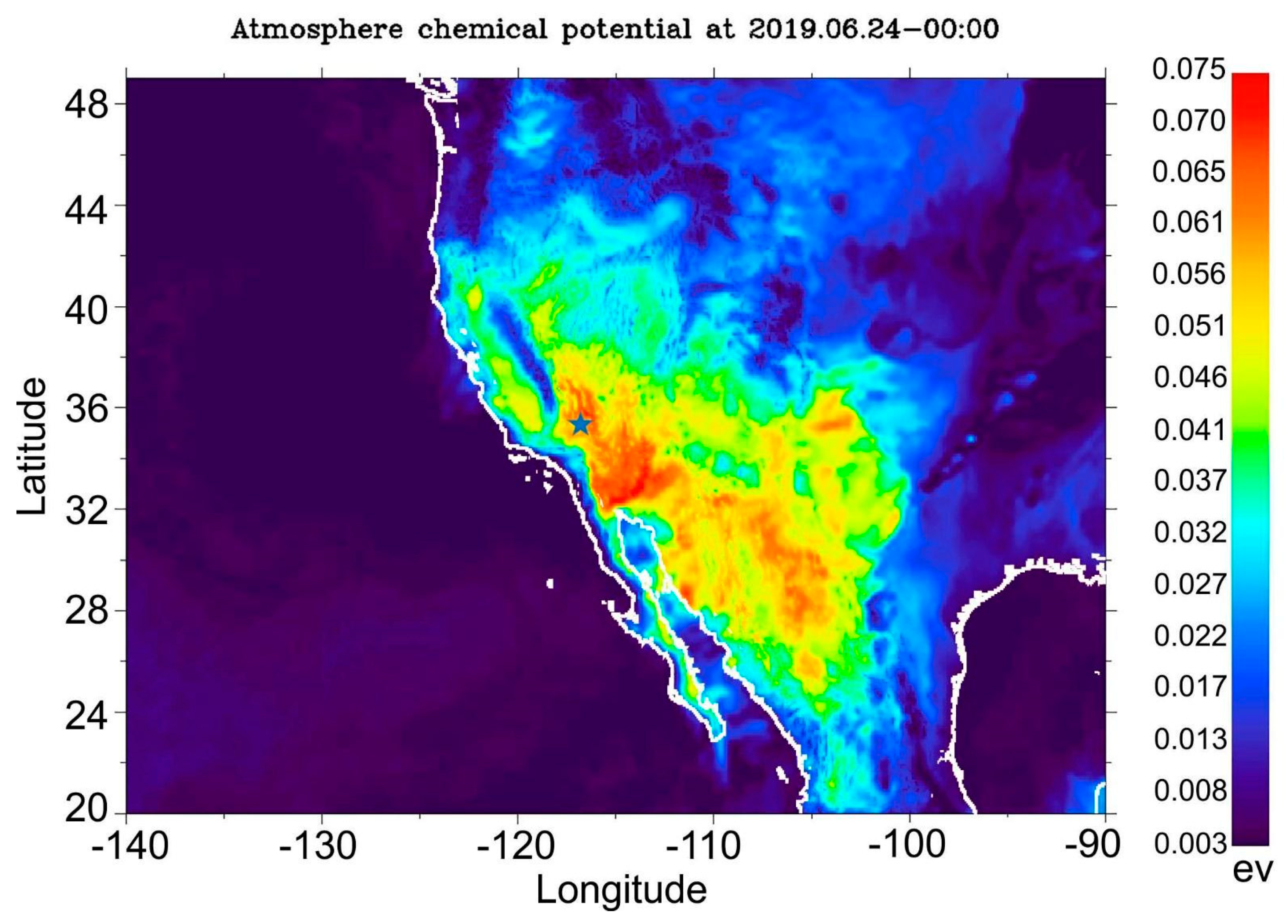
We can add two more reasons which contribute to the non-coincidence of the center of ionospheric distribution and epicenter position. The first one is connected to the physical source through air ionization changes the Global Electric Circuit’s electric properties over the zone of earthquake preparation. This source is the volumetric activity of radon [
4]. The radon activity through the process of air ionization produced by α-particles emitted by radon during its decay leads to sharp changes in the air temperature and relative humidity, which could be monitored by the correction of the chemical potential of water vapor in the atmosphere (ACP) [
4]. Looking at the distribution of the ACP parameter before the Ridgecrest earthquake (
Figure 9), it can be seen that the most intense ACP activity was observed to the south from the epicenter, just close to the maximum of the ionospheric anomaly shown in the upper panel of
Figure 8.
The second reason for the equatorward displacement of ionospheric anomaly from the epicenter of impending earthquake position is connected with the mechanism of electromagnetic seismo-ionospheric coupling. The anomalous electric field changes its direction from vertical to field-aligned, starting from the altitude of 60–80 km. The lower the epicenter latitude, the smaller the magnetic inclination angle, and as the direction taken by the anomalous electric field becomes more horizontal the position of the anomaly mapping within the ionosphere shifts equatorward.
The last proof of the ionospheric precursor locality for the case of the Ridgecrest earthquake we would like to provide the data from the Langmuir probe installed onboard the China Seismo-Electromagnetic Satellite (CSES) which was presented in [
38]. It is interesting to note that the large-scale ionospheric irregularity over California was also registered during the night of 28 June 2019 (
Figure 10). In the upper panel of
Figure 10 one can see the variations of the electron concentration along the orbits registered by the Langmuir probe. The red curve corresponds to the satellite passing over the earthquake preparation zone. The bottom panel shows the distribution of electron concentration over California on DOY 179 (28 June). The CSES satellite has the sun-synchronized orbit with crossing the equator at 14 LT and 02 LT. The night-time passes over California are shown in
Figure 10.
7. Determination of Earthquake Forecast Parameters
After considering the precursors’ behavior in time and space, it is worth discussing the possibility of determining the main forecast parameters: time, place, and magnitude of an impending earthquake.
For both cases, we determined the precursory period (from precursor mask and spatial variability index), which lasted nearly five days. In the Hector Mine earthquake case, the precursory period terminated one day before the mainshock, and in the case of the Ridgecrest earthquake, six days before the mainshock and three days before the foreshock. We obtained 6- and 1-day leading times for the Hector Mine and six days for the Ridgecrest from the cross-correlation coefficients. From the analysis of the ionospheric precursors’ spatial distribution, the most pronounced days revealed the apparent local anomaly was five days before the Hector Mine earthquake and seven days before the Ridgecrest earthquake. In this regard, we should state that we cannot determine the impending earthquake’s time with precision better than 1–7 days before the mainshock. There are plenty of publications with statistical analysis of ionospheric precursors for different regions of the globe [
39,
40] and on a global scale [
41]. Based on the last publication, the largest probability of the ionospheric earthquake precursor lies within the interval 1–7 days, which exactly coincides with our estimations. It should be taken into account that every seismic area has its own characteristics. This means that putting the task of real prediction, the historical study should be undertaken as it was done for Italy [
15], but in any case, the seven days tolerance is much better than any middle-term, and especially long-term, forecast.
Regarding the epicenter position’s determination, it was demonstrated as early as 2003 that the ionospheric precursors have a local character and are “tied” to the anticipated earthquake epicenter position. Li and Parrot [
42] demonstrated the procedure of epicenter position determination from in-situ satellite measurements of electron concentration using mapping of the anomaly registration from several passes of the DEMETER satellite over the seismically active area. The data we have using the GIM data, from which we calculate the differential maps, is similar but continuous in time (
Figure 8, upper panel). We can associate the maximum of the ionospheric anomaly distribution with the earthquake epicenter position. In the Ridgecrest earthquake case we have three sources of information simultaneously: GIM differential map; local network differential map; and in-situ measurements of the electron concentration onboard the CSES satellite. If we associate the probable position of the epicenter with the maximum of the registered anomaly we will get different numbers, but if we calculate the average of the three sources of coordinates we will obtain 35 N and 117.37 W, which against the real values of 35.766 N and 117.605 is not an imperfect estimation.
The earthquake magnitude is based on the idea that the ionospheric anomaly size is the same order of magnitude as the earthquake preparation zone, proposed by Dobrovolsky et al. [
32]. Its radius could be determined as R (km) = 100.43 M, where R is the radius of the earthquake preparation zone, and M is the earthquake magnitude. Many of the magnitude estimation cases are based on differential GIM maps one can find in [
23]. Here we used a modified approach. Instead of differential maps calculated in absolute TEC values, we calculated the percentage differential maps presented in
Figure 8 (upper panel), where the ionospheric anomalies are rounded by some circles based on the Dobrovolsky formula. For the magnitude M7.1, the radius should be 1130 km. To demonstrate that this is a reasonable estimation, we drew the circles with the given radius on both earthquakes’ distributions. One can see that they fall into the range of 20–22% of positive deviation. This coincides with our previous earthquake results in the Kamchatka region [
43]. We can conclude that by estimating the ionospheric anomaly size on the level of deviation 20–22%, we can estimate the earthquake magnitude.
Concluding this paragraph, we can state that data of ionospheric monitoring can allow the estimation of all three parameters necessary for short-term earthquake forecasting with reasonable precision.
8. Discussion
This publication attempts to demonstrate the progress in the technology of the ionospheric precursors of earthquake identification compared with the first attempts [
7,
8,
13]. The Ridgecrest M7.1 earthquake on 5 July 2019 happened precisely 20 years after the Hector Mine earthquake with the same magnitude and in the same region of California, USA, providing a unique opportunity to demonstrate the technological development and its ability to detect the precursors both in quiet and strong disturbing conditions. We have illustrated the uniqueness of the “precursor mask” technology, permitting us to identify the ionospheric precursors even in strongly disturbed conditions, such as existed in October 1999. Simultaneously we demonstrated the close similarity of precursors’ development for the given region and given magnitude. Even the local time of optimal precursor detection is practically the same. The leading time of precursor’s appearance is also the same order of magnitude (11 October, 5 days before, and 28 June, 7 days before the mainshock, but 5 days before the strong foreshock). Within the multiparameter monitoring paradigm [
16], we separated the area of multiparameter ionospheric monitoring where we used several sources of information: vertical ionospheric sounding; GPS TEC from local networks; global GIM maps; and satellite measurements of the space plasma parameters. We also used the multifactor analysis where from the same source, we generated the special detection instruments such as cross-correlation coefficient or spatial variability index, which helped to detect the precursory periods (red lines in
Figure 3 and burgundy rectangles at
Figure 4) and the most sensitive days (minima at cross-correlations coefficient curves at
Figure 7). All together, this has allowed us to detect and identify the ionospheric precursors unequivocally. We did not touch here on the problem of statistical analysis and false alarm determination. The reason is straightforward: this paper’s main task is to demonstrate the precursors’ difference and similarity for two selected earthquakes only. As a hint for future discussion on the false alarm problem, we can say that multiparameter analysis is a cure for false alarms. We can have a similar precursor effect for one parameter, but without an earthquake, to have false indications in many different measurements simultaneously is impossible. Our next goal is to move to the next step: automation of the described procedures to implement our technology in short-term earthquake forecasting.


