Comparison of the Air Pollution Mathematical Model of PM₁₀ and Moss Biomonitoring Results in the Tritia Region

Abstract

Knowing the relationship between pollution sources and air pollution concentrations is crucial. Mathematical modeling is a suitable method for the assessment of this relationship. The aim of this research was to compare the results of the Analytical Dispersion Modelling Supercomputer System (ADMOSS), which is used for air pollution modeling in large areas, with the results of moss biomonitoring. For comparison purposes, air pollution mathematical modeling and the collection of moss samples for biomonitoring in the Czech–Polish–Slovak border area in the European Grouping of Territorial Cooperation (EGTC) Tritia were carried out. Moss samples were analyzed by multi-element instrumental neutron activation analysis (INAA). The INAA results were statistically processed using the correlation-matrix-based hierarchical clustering and correlation analysis of the biomonitoring results and ADMOSS results. Biomonitoring using bryophytes proved to be suitable for the verification of mathematical models of air pollution due to the ability of bryophytes to capture the long-term deposition of pollutants and the resulting possibility of finding the real distribution of pollutants in the area, as well as identify the specific chemical elements, the distribution of which coincides with the mathematical model.

1. Introduction

1.1. Background

Understanding the relationship between pollution sources and air pollution concentrations is crucial for effective air quality management. Mathematical modeling is an appropriate method for the assessment of this relationship, however, it is necessary to take into consideration that various types of errors occur during mathematical modeling:

• Problem formulation error;
• Real-world abstraction error;
• Inputting data error;
• Human factor error;
• Rounding error.

Therefore, a comparison of modeling results with real measured concentrations is required. The ADMOSS includes standard air pollution monitoring in the modeling process. Consequently, it is essential to use alternative methods, including biomonitoring. The present study brings a unique approach to the verification of air pollution mathematical modeling using a comparison of the results of mathematical modeling and moss biomonitoring. In the literature, there was only one study which the authors found that compared mathematical modeling results and biomonitoring results [1]. Based on this fact, the given issue can be considered unsurveyed. This study is based on the research published in the Ph.D. thesis [2].

1.2. Air Pollution

Air pollution is an undesirable phenomenon that entails a multitude of negative health, economic and social impacts [3,4,5]. Previous studies show that PM has significant adverse effects on human health in the form of black lungs, asthma, cardiovascular diseases and lung cancer [6,7,8]. The process that causes air pollution is called polluting. Polluting the air is a process of emitting pollutants into the air from pollution sources (emissions). A pollutant is any substance that can harm the health of organisms, ecosystems or cause irritation by odor (Act No. 201/2012 Coll., on air protection) [9]. Sources are anthropogenic or natural. The characteristic properties of natural sources are their equal distribution in a large area (lightning—NO_x; forest fires—NO_x; PM_x; volcanic activity—PM_x; SO₂, etc.). Anthropogenic pollution is related to human activities, and pollution sources are usually concentrated in inhabited areas [5]. This study focuses on particulate pollution.

1.3. Air Pollution Protection and Modeling

Air protection is the prevention of and reduction in pollutants so that they are not harmful to human health, the environment and ecosystems. The creation of suitable conditions for the regeneration of already damaged components of the environment is also part of air protection. Air quality in the Czech Republic is monitored by air pollution monitoring stations, which perform standard measurements of air pollution concentrations. The law on air protection (Act No. 201/2012 Coll., on air protection) [9] defines the maximum permitted concentrations for specific substances, i.e., limit values. If the limit values are exceeded, the current air quality management system, intermediate air quality developments and expected scenarios of polluting need to be evaluated. The mathematical modeling of air pollution is an ideal tool for evaluating these scenarios [10]. Subsequently, suitable strategies to reduce air pollution are to be determined on the basis of relevant information.

1.4. Study Area

The survey focused on the verification of the model in the area of interest of the AIR TRITIA project [11,12]. This project deals with the issue of air quality management in the European Grouping of Territorial Cooperation (EGTC) Tritia (Figure 1). The region comprises the Moravian-Silesian Region (Czech Republic), the Opole Voivodeship, the Silesian Voivodeship (Republic of Poland) and the Žilina Region (Slovak Republic). Its area is 34,069 km² with a population of approximately 7.8 million.

The Moravia–Silesian Region is located on the southwestern side of the EGTC Tritia. It borders the Silesian Voivodeship in the east, the Opole Voivodeship in the north and the Žilina Region in the southeast. The most important geomorphological formations in the EGTC Tritia area are the Bohemian Massif and the Western Carpathians. Between these two formations, there are the Moravian Gate and the Ostrava Basin, which turn into the Silesian Lowland in the east and northeast, with the Odra River flowing through. The southern part of the territory is mountainous because the Western Carpathians massif originates from there. The Váh river valley passes through this massif [13,14].

The regions grouped into the EGTC Tritia combine common environmental and social problems and intensive socio–economic relations. Given the high population density, improving air quality is a crucial issue for these regions.

2. Material and Methods

2.1. Mathematical Modeling

Air pollution monitoring provides information on air quality only in measurement points, where each monitoring site represents its limited vicinity. The pollution monitoring station network is also usually rather sparse since professional monitoring equipment is costly and demands professional calibration and maintenance [15]. Mathematical modelling is an important tool that complements air quality monitoring. It provides more detailed information on the spatial distribution of air pollution in the area of interest. It can also provide information on the share of various air pollution source groups on air quality and allows studying the effects of “what if” scenarios.

Air pollution models can be classified according to various criteria. Based on the time component, models can be divided into static and dynamic. Static models do not take time into account. The model classification according to the most frequently used types is more detailed [16]:

• Empirical;
• Gaussian;
• Numerical;
• Physical.

This classification is the most general, dividing models into groups based on the general principle of constructing the model. A more subtle classification can be created for each category listed above. For example, numerical models are usually classified into Lagrangian, Eulerian and chemical balance models.

This article focuses on the verification of the Gaussian model. Gaussian models are mathematically based on Sutton’s diffusion theory (Sutton [17]) which is derived from the equations for the Lagrange function in order to represent atmospheric diffusion. The diffusion of pollutants in the axis x direction is characterized by the parameters C_y, C_z. These parameters are derived on the basis of Taylor’s statistical correlation theory of turbulence and the classical diffusion equation.

To evaluate air quality in large areas, the Analytical Dispersion Modelling Supercomputer System (ADMOSS) was developed at the VSB—Technical University of Ostrava (VSB-TUO). The ADMOSS system uses Geographic Information System (GIS), a mathematical model and computing clusters. Currently, the ADMOSS system uses the SYMOS’97 methodology for the mathematical modeling of air pollution. The SYMOS’97 modeling methodology is a Gaussian dispersion model recommended by the Ministry of the Environment of the Czech Republic for assessing the effects of gas or dust emissions. The methodology is capable of evaluating the degree of air pollution by gases and solid pollutants that are released by point, linear or area sources. Pollution values are computed in a network of reference points called receptors. SYMOS’97 calculates the atmospheric pollution characteristics based on the following input data [18]:

• Data describing the sources of air pollution;
• Data describing the receptor point network;
• Data describing the terrain;
• Meteorological characteristics of the modeled areas and time period.

These several characteristics can be calculated for each point:

• Maximum possible short-term (hourly) air pollution concentrations in all wind flow velocity and air stability classes;
• 8 h moving average;
• Annual average concentrations;
• Duration of exceeded limit values (pollution limits);
• Particulate deposition.

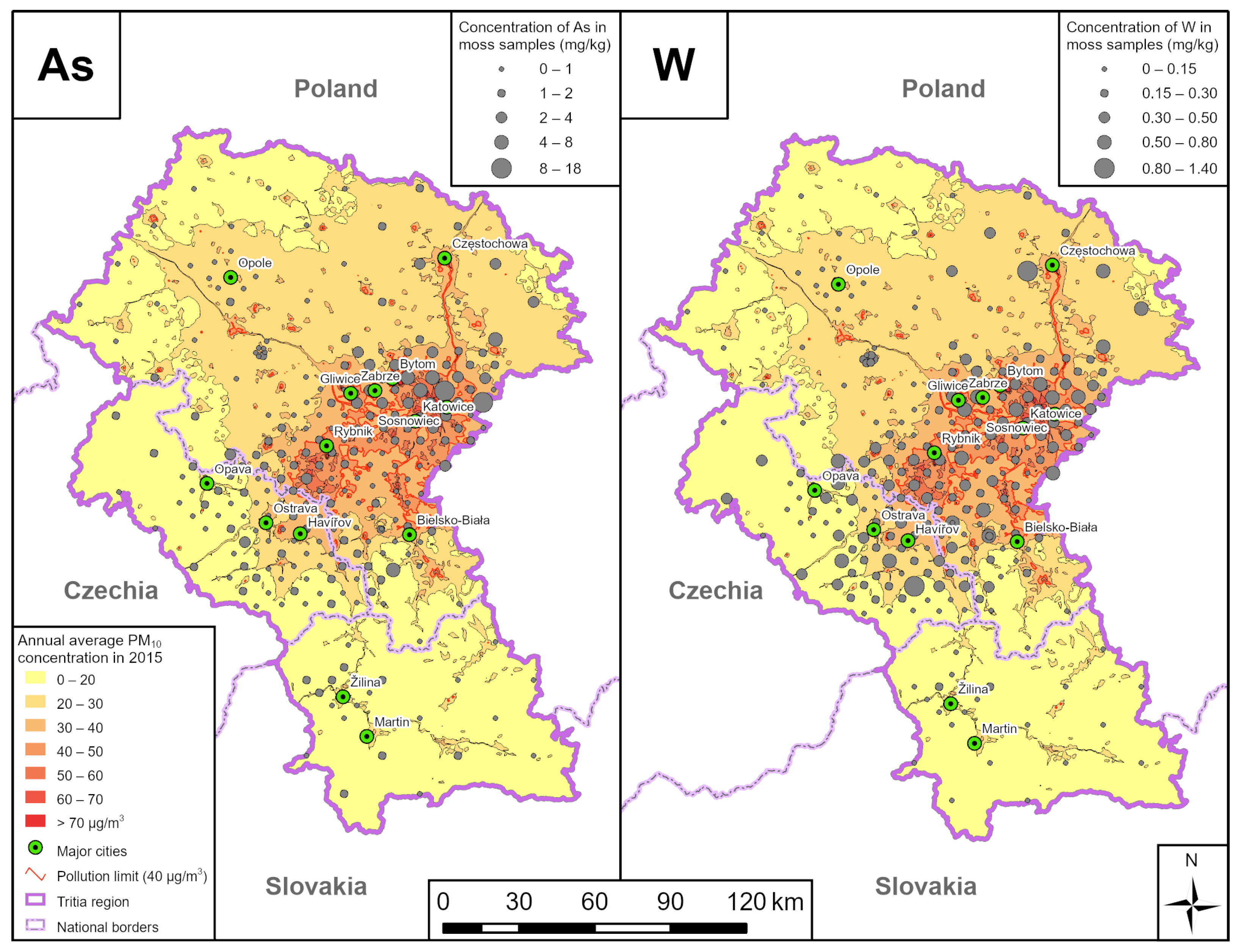
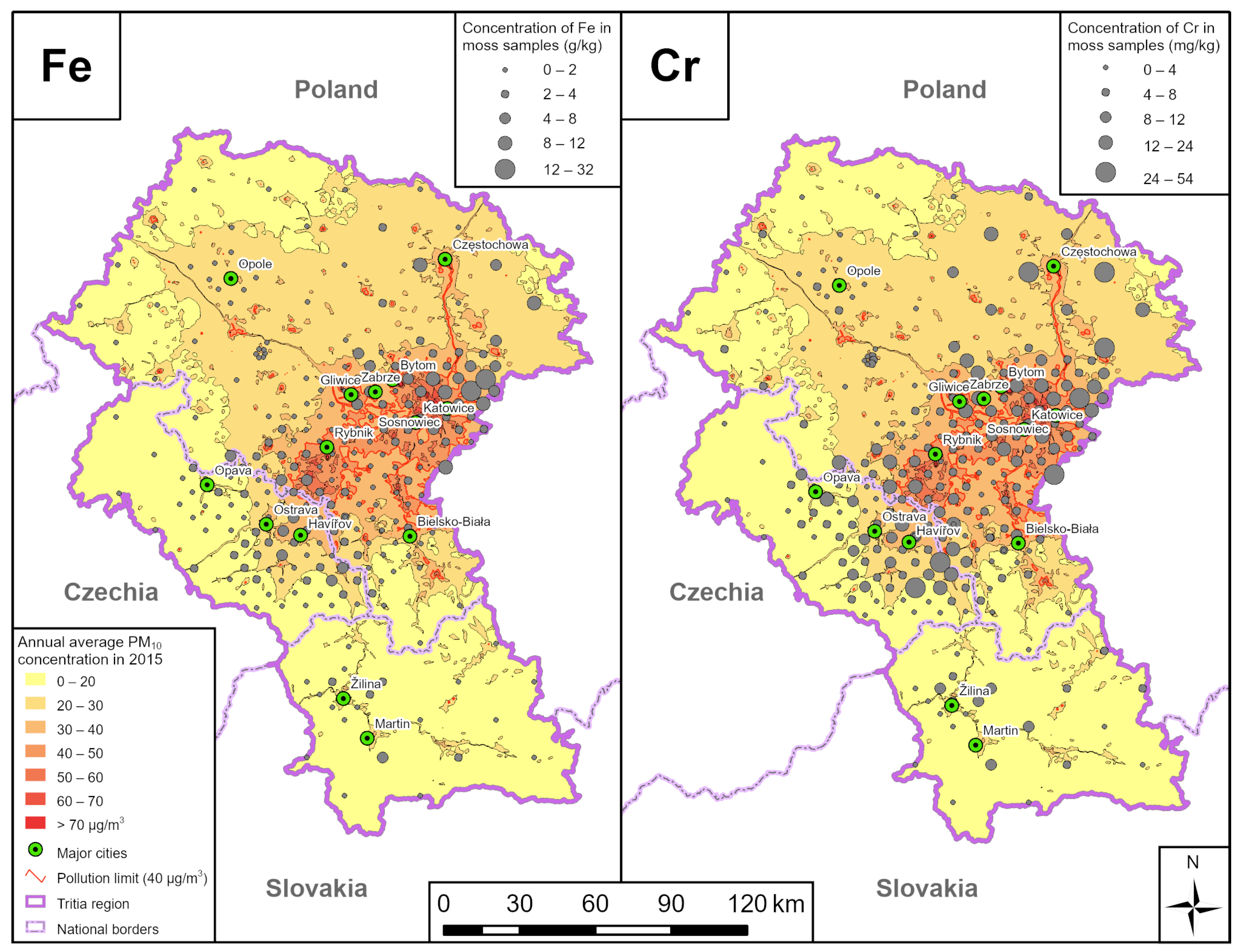
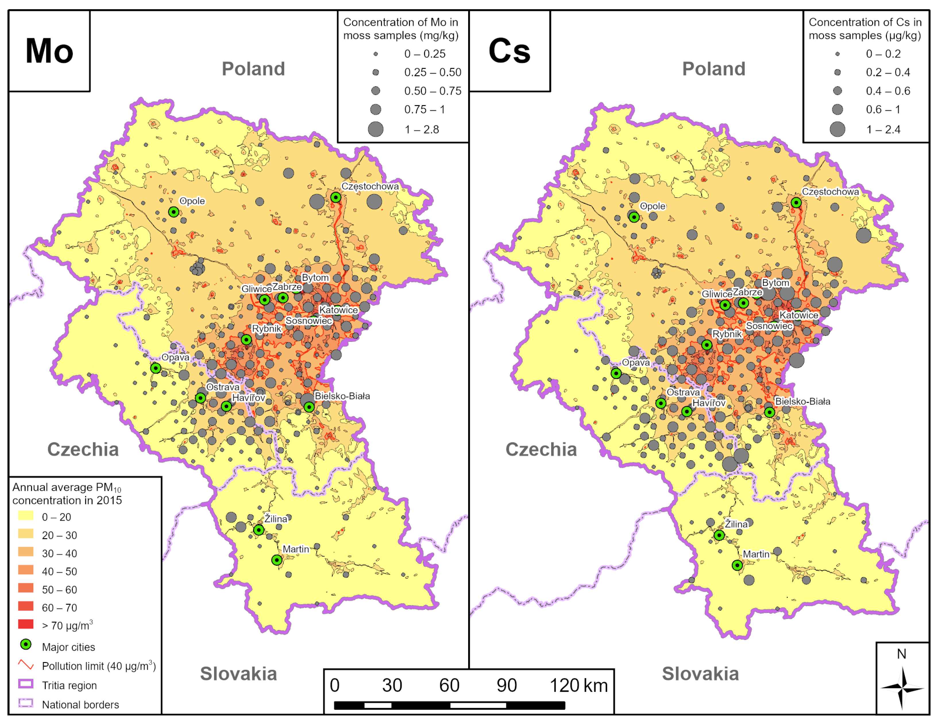
For this analysis, a PM${}_{10}$ deposition model was computed. PM${}_{10}$ was chosen because suspended particles with a diameter of 10 micrometers deposit on the Earth’s surface or vegetation with a decreasing diameter, and this phenomenon is less significant. In Leoni et al. [19], the authors studied the origin and chemical composition of dust particles from samples collected in the vicinity of Liberty’s steelworks in Ostrava. The PMF analysis detected the association of several chemical elements in dust particles with pollution sources. Coal combustion was responsible for the S, As, Se, and Br concentrations, the origin of Al, Si, Ca, Ti, and Cu came from the Earth’s crust, Na, Cl and Zn originated from sintering and steel production, and Mn, Fe and Co corresponded with raw iron production.

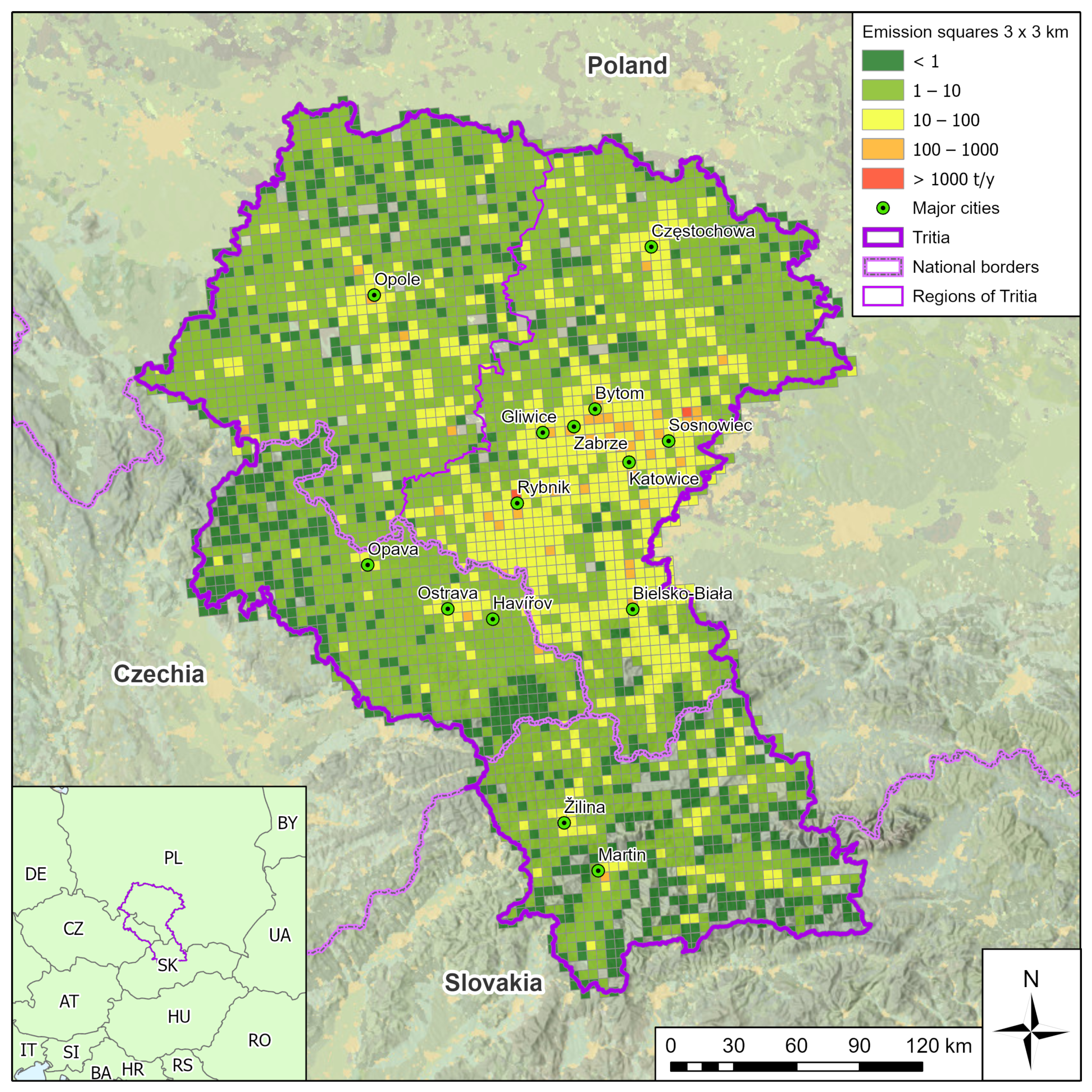
The input data for the model were obtained from the Air Tritia [11,12] dataset, AND the modeling year was 2015. The receptor point network was generated from the coordinates of the sampling sites. This made it possible to compare the moss survey results and deposition model results. The emission data used in modeling are summarized as follows in

Table 1. Emission of PM${}_{10}$ in the area of interest.

Country	Pollution Sources	No. of Sources	Emission (t/y)
Czech Republic	Industrial sources	4728	1325
	Domestic heating	52,669	1225
	Car traffic	59,651	514
Poland	Industrial sources	17,485	9962
	Domestic heating	131,741	20,603
	Car traffic	403,451	1965
Slovakia	Industrial sources	1366	233
	Domestic heating	33,576	2686
	Car traffic	34,009	301
	Total	738,676	38,814

and Figure 2.

The modeling data were corrected by the pollution monitoring data. Two correction coefficients (additive + multiplicative) were added. The additive coefficient represents air pollution from all pollution sources that were not considered in the model, i.e., natural sources, long-range pollution transport, etc. The multiplicative coefficient is a correction of the model (the SYMOS’97 model is known to underestimate pollution), as well as a correction of emission data (emissions can be under- or overestimated) and secondary pollution.

The modeling results can be considered reliable in the vicinity of pollution monitoring stations. However, there are relatively few such stations in the vast monitoring area, so additional model verification is valuable.

2.2. Moss Survey

At present, there are many traditional direct methods for monitoring air pollution. These methods are often costly, hindering extensive long-term studies. Thus, there is space for indirect monitoring methods, including biomonitoring. Biomonitoring refers to the use of organisms (plants, fungi or animals) to assess the condition of the biosphere [20]. Information is obtained by studying the behavior of the organism, the presence of substances in the body, or simply by the presence of the organism. These organisms are called bioindicators. A properly selected bioindicator should reflect and cumulate the monitored element quantitatively and qualitatively (occurrence, color, shape, size). Therefore, grass [21], tree leaves [22], human tissues [23], bryophytes [24], lichens [25], or wood [26] can be used as bioindicators.

Bryophytes are ideal bioindicators of air pollution due to their specific properties. Bryophytes receive only a small amount of nutrients through the root system since they are not rooted in the substrate [27,28]. The intake of substances from the soil can be completely eliminated by active biomonitoring. This is based on the exposure of known bioindicators to the influences in the monitored area and on the monitoring of their reaction or subsequent analysis.

A long-term survey of the atmospheric deposition of heavy metals using bryophytes in Sweden was carried out between 1968 and 1995. The study focused on elements related to metallurgical industry and combustion processes (Cd, Cu, Fe, Pb, Hg, Ni, Va and Zn). A decrease between 1968 and 1995 was recorded for Fe (80%), Pb (89%), Cd (76%), Ni (72%), Hg (69%), V (57%), Zn (49%) and Cu (48%) [29,30].

Within 1985 and 2000, a heavy metal deposition study (Cd, Cr, Cu, Fe, Ni, Pb, Zn, V, As and Hg) was conducted in Finland. In total, 1569 sampling sites were monitored at the beginning and 2000 sampling sites at the end. The Pb (78%), V (70%) and Cd (67%) values decreased during the monitored period. For the other elements, a decrease between 16 and 34% was observed [31].

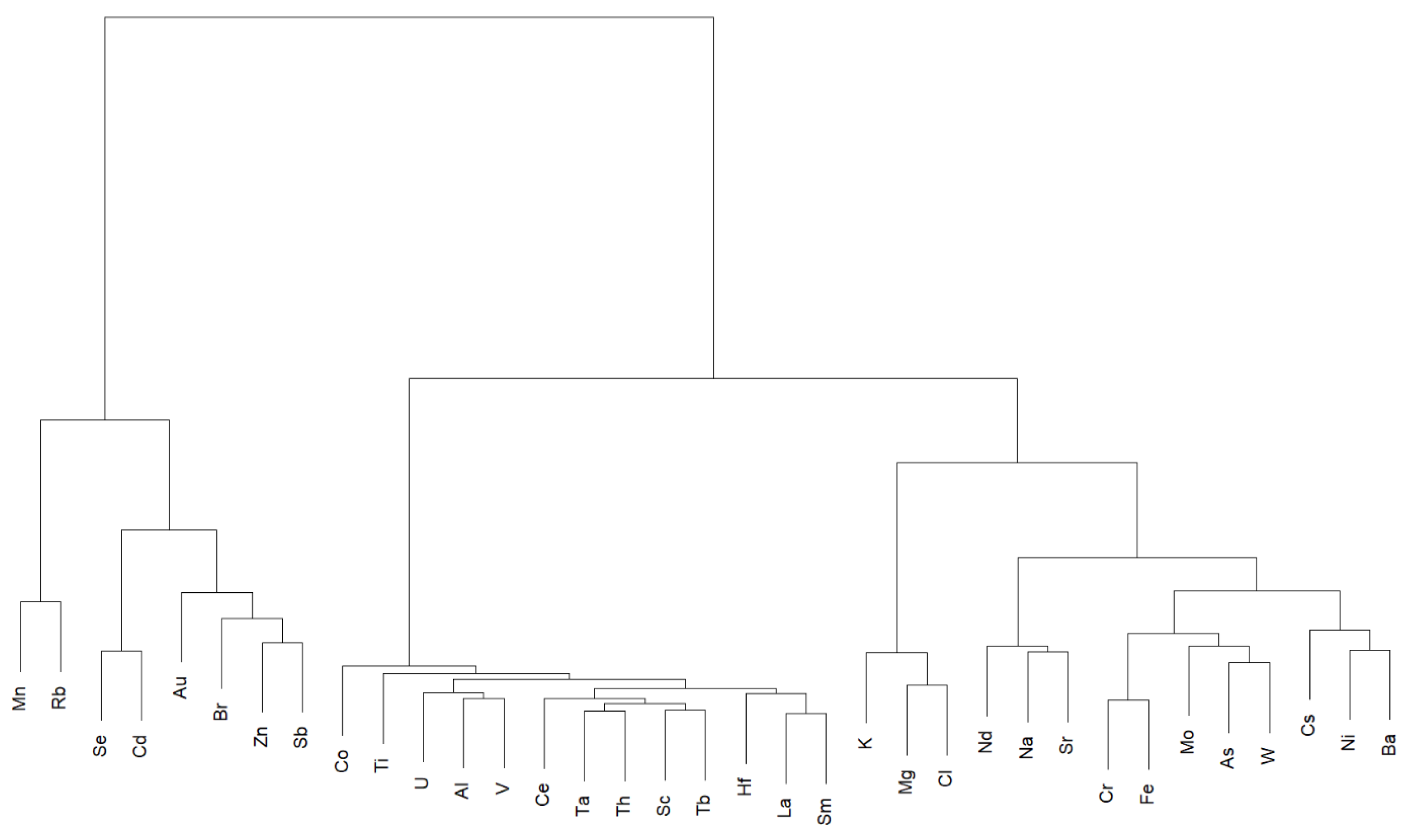
Frontasyeva [24] use instrumental neutron activation analysis (INAA) to analyze the bryophyte samples [32]. By means of INAA, the team of JINR’s Frank Laboratory of Neutron Physics (FLNP) is able to determine mass concentrations of up to 45 elements of Ag, Al, As, Au, Ba, Br, Ca, Ce, Cl, Co, Cr, Cs, Dy, Eu, Fe, Hf, Hg, I, In, K, La, Lu, Mg, Mn, Na, Nd, Ni, Rb, Sb, Sc, Se, Sn, Sm, Sr, Ta, Tb, Ti, V, U, W, Yb, Zn and Zr. However, elements such as Cd, Cu, Hg, and Pb, important for environmental studies, can be additionally determined using Atomic Absorption Spectroscopy (AAS).

Biomonitoring using bryophytes was carried out in the Czech Republic by the Research Institute of Ornamental Gardening (RIOG). Various elements were analyzed within 1991/1992, 1995/1996, 2000/2001, 2005/2006 and 2010. In total, 273 sampling sites were monitored, and the concentrations of Ag, Al, As, Ba, Be, Bi, Cd, Ce, Co, Cr, Cs, Cu, Fe, Ga, In, La, Li, Mn, Mo, Nd, Ni, Pb, Pr, Rb, S, Sb, Se, Sn, Sr, Th, Tl, U, V, Y and Zn was measured in 2010 [33,34].

Biomonitoring is widely used to assess air pollution in large areas, especially in Europe and Asia. That is why biomonitoring is a suitable method for verifying the results of the Analytical Dispersion Modelling Supercomputer System (ADMOSS). Since 2014, the VSB-Technical University of Ostrava (VSB-TUO) has been participating in the project of the International Cooperative Programme on Effects of Air Pollution on Natural Vegetation and Crops (ICP Vegetation) [35], which aims to assess the impact of air pollution on vegetation. The ICP Vegetation project started in the 1980s. Currently, scientific teams from more than 40 countries are involved. The Joint Institute for Nuclear Research (JINR) in Dubna is one of the organizations participating in this project.

The ICP Vegetation project focuses on the impact of air pollution in large areas (at the continental scale). Investigations conducted by the VSB-TUO team applied the principles of ICP Vegetation at a regional scale to identify specific source groups.

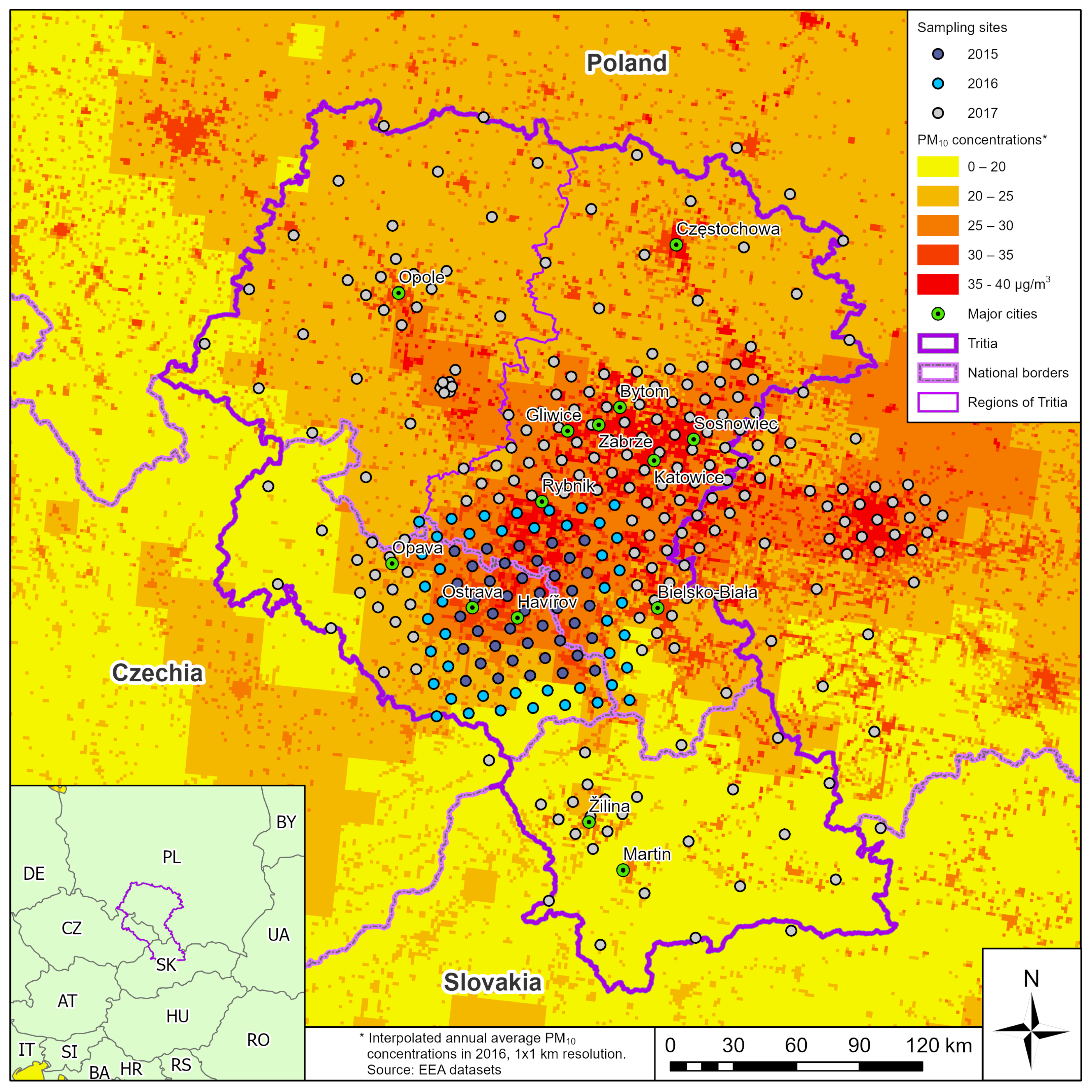
In 2015, based on the results of the AIR SILESIA project [36], a sampling area of 1600 km² (40 × 40 km) in the center of the polluted area in the Czech-Polish border area was selected. A regular network of 41 sampling points was established in the selected area. In 2016, the original sampling network was extended by 44 more sampling sites. In June 2017, the last 244 samples were taken. 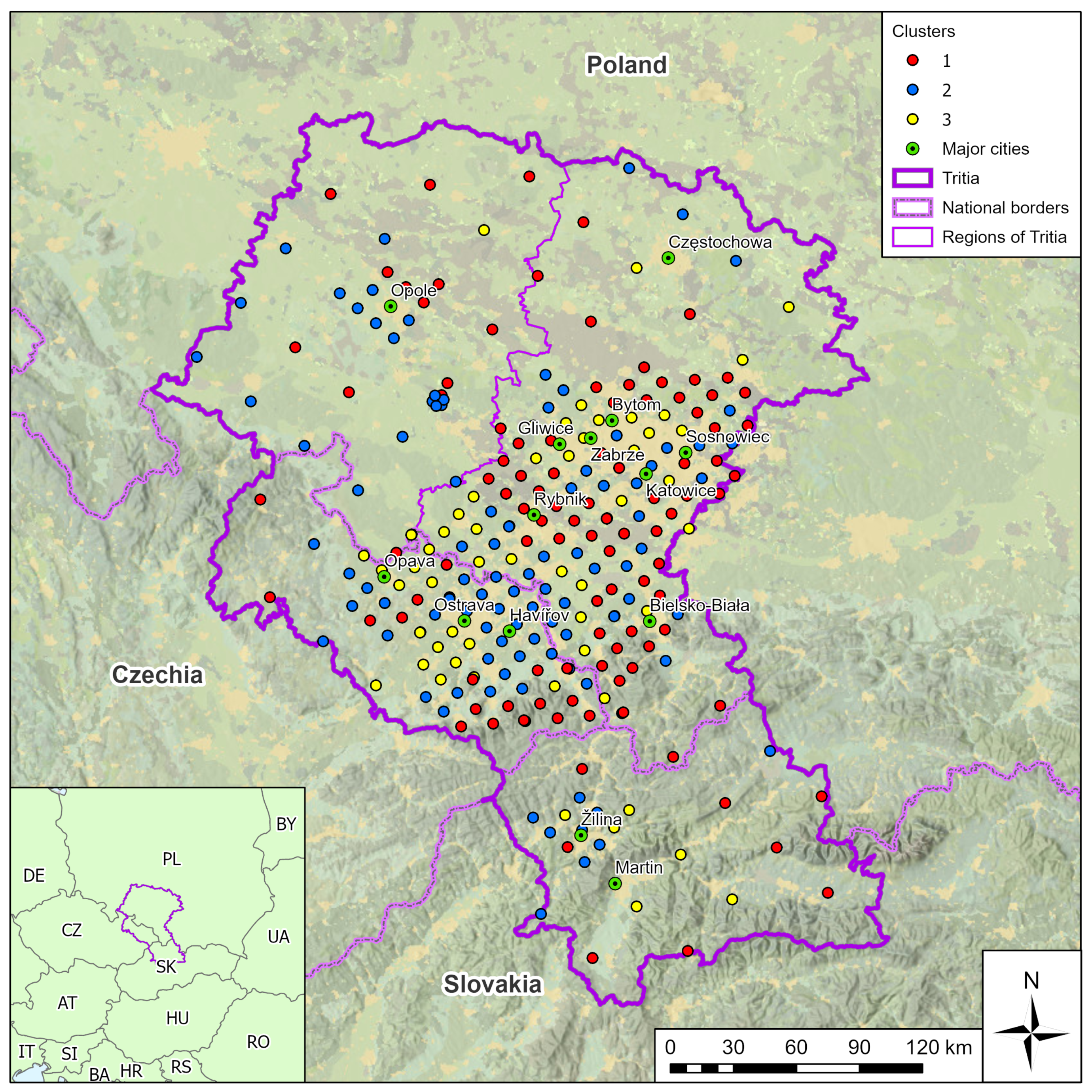In the area of interest of the AIR TRITIA [11,12] project, covering an area of 36,000 km² and its surroundings, an irregular collection network was created (Figure 3). This sampling network encompasses the measurements of air pollution monitoring, mathematical modeling and previous collection campaigns carried out by VSB-TUO. The collection network consists of a regular 20 × 20 km collection network, which is concentrated in areas with an expected higher gradient of pollutant concentrations by a 7 × 7 km network. Within 2015, 2016, and 2017, 285 moss samples were collected in the area of interest of the Air Tritia project.

2.3. Instrumental Neutron Activation Analysis

The collected mosses were analyzed using INAA, which belongs to the analysis recommended by the ICP Vegetation guideline. INAA is a radiological analytical method in which a sample of interest is placed in a neutron field. INAA is not sensitive to the bonding between elements or to the oxidation state of the analyzed substance. It provides qualitative and quantitative information about the analyzed substance. INAA is a non-destructive method, which makes it ideal for analyzing, for example, archaeological or biological samples [24,37].

At JINR, INAA is carried out at the IBR-2M research pulse reactor [38] using the REGATA experimental device. This device is utilized to irradiate and measure the gamma spectra of irradiated samples. To activate the sample, it must be put into the neutron beam generated by the reactor. Since this is a comparative method, it is also necessary to irradiate the considered standard of the detected elements. The quality control of the INAA results was ensured by the simultaneous analysis of the examined samples and standard reference materials (SRM) of the National Institute of Standards and Technology (NIST) and the Institute for Reference Materials and Measurements (IRMM): NIST SRM 1515—Apple Leaves, NIST SRM 1547—peach leaves, NIST SRM 1573a—tomato leaves, NIST SRM 1575a—pine needles, NIST SRM 1633b—coal fly ash, NIST SRM 1633c—coal fly ash, NIST SRM 1632c—coal (bituminous), NIST SRM 2709—San Joaquin soil, NIST SRM 2710—Montana soil, NIST SRM 2711—Montana soil, SRM 2891—copper sand, IRMM BCR 667—estuarine sediment. The interaction of nuclei and neutrons creates unstable radionuclides that emit characteristic gamma radiation for individual elements. This radiation can be detected [39].

Then, the activated sample was removed from the neutron field using a pneumatic system, and its activity was detected in the laboratory environment by HPGe detectors. Since the samples emit ionizing gamma radiation, this process is automated. The result was a gamma spectrum of the sample. This spectrum was then processed by a specialist in special software (GENIE), who also received all the relevant information from the measured spectrum (percentage uncertainty of the measurement, area of individual peaks and measurement time). The individual elements differ in the energy and intensity of the gamma rays emitted. Knowing the spectra of the weighed standard and the sample, one can calculate the mass concentrations of individual elements.

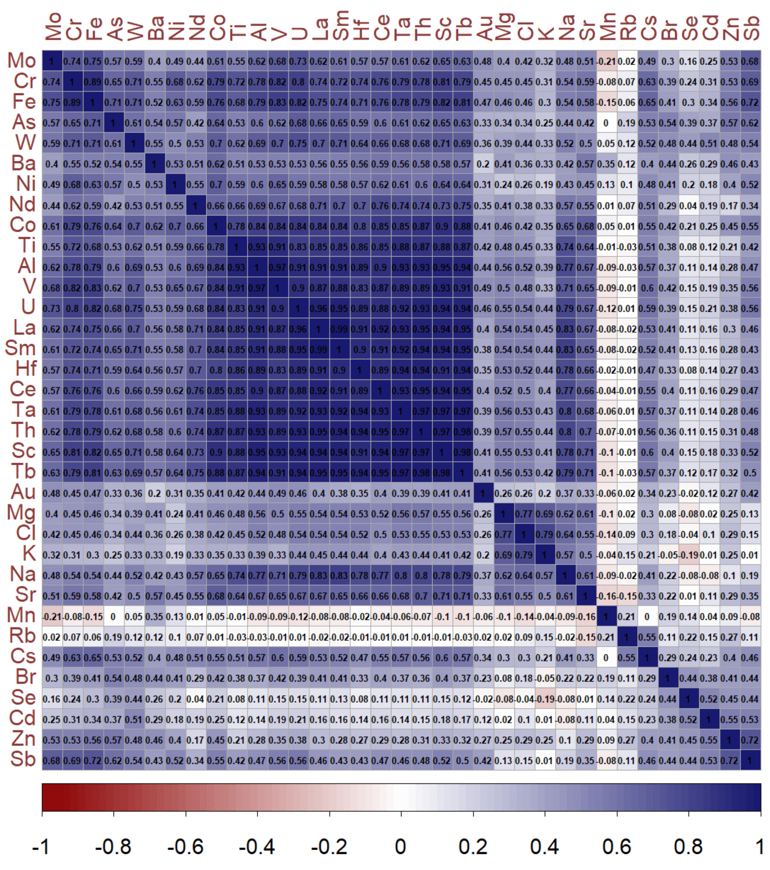
As a result of INAA, mass concentrations of about 40 elements were obtained (the number is variable—

Table 2. Number of analyzed chemical elements for each year.

Year	Number of Analyzed Chemical Elements
2015	38
2016	47
2017	35

). These results were further processed statistically, and a comparison with the modeling results was performed in the Geographic Information System (GIS).

2.4. Statistical Analysis

2.4.1. Exploratory Data Analysis

Statistical distributions of environmental data expressing concentrations are usually left-skewed (inclined to lower values than average) and do not fit the assumption of normal distribution. The Shapiro–Wilk test was used to refute this assumption. The test was implemented in the R environment. This function allows testing selections ranging from 3 to 5000 values [40].

2.4.2. Correlation Analysis

The next step is to perform a correlation analysis. First of all, the correlation between individual chemical elements was investigated. Spearman’s rank correlation coefficient was chosen for that. The correlation analysis results can be displayed in a correlation matrix. The clusters of chemical elements can be visually identified in the correlation matrix. The best way to do this is to display the clusters using a dendrogram [41].

The concentrations computed by the ADMOSS system were checked at the points where bryophyte samples were collected. Using the ST_Value function, the total concentrations and contributions of individual resource groups were extracted from the rasters (modeling results). The extracted values were saved in a separate table. This table was further used in the R environment. The correlation between the INAA results and individual groups of pollutant sources was examined. Spearman’s rank correlation coefficient was used to assess this dependence [41,42].

2.4.3. Hierarchical Clustering on Principal Components (HCPC)

INAA results in mass concentrations of elements. They are shares of the whole and carry relative information. Therefore, this is compositional data, or a composition. The sum of the data contained in the composition is bounded from above by the constant K. The individual components of the composition can have values of 0 and higher. Standard statistical methods assume that the data are elements of the Euclidean space, i.e., they can take arbitrary values without limitation. The compositional data do not meet this condition, the constraints described above guarantee that all permissible values constitute a subset of the Euclidean space called a simplex (2D triangle, 3D tetrahedron). In this case, standard statistical procedures can lead to incorrect results. For the statistical analysis of the compositional data, it is therefore necessary to perform a mathematical transformation that converts the compositional data vector into a vector of new values that no longer have the aforementioned spatial constraints. Aitchison transforms are used for this purpose; in this work, the centered log ratio transformation (CLR) was chosen [43].

For multidimensional data files, it is appropriate to perform dimensional reduction for cluster analysis and the subsequent interpretation of the results. For this, principal component analysis (PCA) is used. By analyzing the main components, the existing variables are replaced by fewer other mutually independent variables, with as minimal information loss as possible. Further computations involve those components that have an eigenvalue greater than or equal to 1. The remaining components were considered statistical noise, reducing cluster stability. Hierarchical clustering on principal components (HCPC) is performed on these selected components [43].

3. Results

3.1. INAA

3.1.1. Exploratory Data Analysis Results

The results of bryophyte analysis by INAA provide information on the mass concentration of individual chemical elements in the examined samples. These results were imported into a PostgreSQL database, and the data were subsequently processed in the R statistical environment [44]. From the calculated characteristics (

Table 3. Basic statistical characteristics of the INAA results.

	Min. Conc.	Max. Conc.	Range	Median	Mean	Variance	Skew
	(mg/g)	(mg/g)	(mg/g)	(mg/g)	(mg/g)	(mg/g)2	/
Na	47.5	1790	1742.5	185	243.33	48,551.78	3.57
Mg	569.42	5654.87	5085.45	1760	1933.33	870,363.5	0.96
Al	305	22,600	22,295	1470	2364.16	6,842,151	3.28
Cl	26	2240	2214	237	340	97,047.3	2.44
K	3740	20,200	16,460	9480	9686.68	10,864,937	0.60
Sc	0.05	3.8	3.75	0.31	0.48	0.24	2.89
Ti	0.17	2200	2199.83	131	210.52	63,470.53	4.23
V	0.55	34	33.45	2.6	3.97	14.27	3.11
Cr	0.02	54	53.98	5.2	7.04	39.51	3.03
Mn	29.5	12,100	12,070.5	194	291.11	456,893.5	14.91
Fe	294	32,000	31,706	1420	2153.51	6,393,958	5.82
Ni	0.32	15.3	14.98	2.86	3.29	4.38	2.53
Co	0.12	4.7	4.58	0.59	0.79	0.39	2.26
Zn	26	1010	984	93	133.2	15,110.45	2.53
As	0.29	18	17.71	0.96	1.28	1.84	7.25
Se	0.02	2.39	2.37	0.38	0.47	0.12	2.32
Br	0.75	9.4	8.65	3.2	3.49	2.06	1.12
Rb	3.2	64	60.8	13	15.33	94.95	1.87
Sr	5.65	89	83.35	24	26.23	176.54	1.27
Mo	0.02	2.8	2.78	0.31	0.38	0.08	3.15
Cd	0.02	13.2	13.18	0.82	1.51	3.39	2.50
Sb	0.05	15.3	15.25	0.36	0.64	1.32	8.42
Ba	7.9	500	492.1	53.9	61.38	1676.69	4.56
Cs	0.02	2.4	2.38	0.29	0.39	0.1	2.35
La	0.19	15	14.81	1.02	1.56	2.99	3.67
Ce	0.01	22	21.99	2.09	3.08	9.82	2.66
Nd	0.09	13.3	13.21	1.48	1.94	2.69	2.31
Sm	0.03	2.27	2.24	0.16	0.25	0.07	3.38
Tb	0	0.37	0.37	0.02	0.04	0	3.69
Hf	0.02	4	3.98	0.22	0.4	0.29	3.78
Ta	0	0.34	0.34	0.03	0.05	0	2.71
W	0.01	1.38	1.37	0.17	0.22	0.03	2.50
Au	0	0.07	0.07	0	0	0	12.53
Th	0.05	3.2	3.15	0.29	0.45	0.23	2.48
U	0	1.07	1.07	0.11	0.17	0.02	2.14

), it was evident that the obtained concentrations of individual chemical elements showed a rather asymmetric distribution skewed to the left.

Since many statistical tests work with the assumption of normal distribution, the normality hypothesis must be upheld or rejected. Based on the low p-value, the data normality hypothesis was rejected for all analyzed elements (

Table 4. Results of the Shapiro–Wilk test for normality.

Chemical Element	W	p-Value	Chemical Element	W	p-Value
Na	0.642358	5.07 × 10${}^{-24}$	Sr	0.916441	1.61 × 10${}^{-11}$
Mg	0.927164	1.36 × 10${}^{-10}$	Mo	0.763946	6.1 × 10${}^{-20}$
Al	0.680549	7.15 × 10${}^{-23}$	Cd	0.700734	3.2 × 10${}^{-22}$
Cl	0.76143	4.85 × 10${}^{-20}$	Sb	0.344264	1.05 × 10${}^{-30}$
K	0.96551	2.51 × 10${}^{-6}$	Ba	0.715013	9.67 × 10${}^{-22}$
Sc	0.708619	5.86 × 10${}^{-22}$	Cs	0.80423	3.09 × 10${}^{-18}$
Ti	0.616256	9.4 × 10${}^{-25}$	La	0.647549	7.17 × 10${}^{-24}$
V	0.729884	3.21 × 10${}^{-21}$	Ce	0.723043	1.84 × 10${}^{-21}$
Cr	0.71803	1.23 × 10${}^{-21}$	Nd	0.81013	5.76 × 10${}^{-18}$
Mn	0.17168	1.64 × 10${}^{-33}$	Sm	0.67519	4.86 × 10${}^{-23}$
Fe	0.557595	2.88 × 10${}^{-26}$	Tb	0.647205	7.01 × 10${}^{-24}$
Ni	0.787189	5.49 × 10${}^{-19}$	Hf	0.604475	4.52 × 10${}^{-25}$
Co	0.790127	7.34 × 10${}^{-19}$	Ta	0.711366	7.26 × 10${}^{-22}$
Zn	0.731635	3.7 × 10${}^{-21}$	W	0.781392	3.12 × 10${}^{-19}$
As	0.469904	2.92 × 10${}^{-28}$	Au	0.13073	4.15 × 10${}^{-34}$
Se	0.743959	1.04 × 10${}^{-20}$	Th	0.721783	1.66 × 10${}^{-21}$
Br	0.931383	3.32 × 10${}^{-10}$	U	0.782747	3.56 × 10${}^{-19}$
Rb	0.842066	2.21 × 10${}^{-16}$

).

3.1.2. Correlation Analysis Results

Consequently, correlation analysis was performed. First, the correlation between individual chemical elements was investigated in the INAA results. Since the hypothesis of data normality was rejected for all chemical elements, it was required to use a non-parametric method to determine the correlation coefficient. Spearman’s rank correlation coefficient corresponded to this criterion. The result was a correlation matrix (Figure 4).

Then, correlation-matrix-based hierarchical clustering (CMBHC) was performed. Three major clusters were identified by CMBHC (Figure 5). The first cluster contained Mn, Rb, Se, Cd, Au, Br, Zn and Sb. This is probably due to natural factors. The second cluster comprises Co, Ti, U, Al, V, Ce, Ta, Th, Sc, Tb, Hf, La and Sm. The concentrations of elements from this cluster could be probably influenced by the soil particles [45]. The last cluster consists of two groups. The first subgroup of elements consists of K, Mg, Cl. The second group contains Nd, Na, Sr, Cr, Fe, Mo, As, W, Cs, Ni and Ba. This cluster, except for Cs, probably involves the impact of human activity. According to Sucharová et al. [34] or Frontasyeva [24], the presence of these elements in bryophytes may be associated with metallurgical processes, coal combustion and mining. The occurrence of Cs is not generally caused by anthropogenic sources in the study area. A probable source of Cs pollution is the Earth’s crust [34].

Map outputs were created on the basis of the INAA results. Cr, Fe, Mo, As, W, Ni and Ba were chosen for a detailed study of spatial distribution (Figure 6, Figure 7, Figure 8 and Figure 9). The distribution of these elements in the Tritia region is similar. All the selected elements show increased values in the Katowice area. All the selected chemical elements, except for As, show increased concentrations in the vicinity of Częstochowa. Increased concentrations of Mo, W and Fe are observed in the Ostrava-Karviná agglomeration. In the area between the towns of Bohumín and Rybnik, there is a locality where all the selected chemical elements, with the exception of As, are elevated.

Furthermore, the interdependence between the INAA results and the results of mathematical modeling using the ADMOSS system was investigated. The first step was the extraction of concentrations calculated by mathematical modeling at the points where moss samples were collected. From the results of the mathematical model, total concentrations, concentrations caused by the influence of industrial sources, concentrations caused by the influence of domestic heating and concentrations caused by the influence of transport were extracted. Spearman’s rank correlation coefficient was used to assess the interdependence since the INAA results do not show normal distribution. Elements correlating with the model had a correlation coefficient greater than 0.3 [42]. In the overall model, Al, Sc, Tb, V, Cl, Cs, Cr, Cd, U, Fe, W, Zn, Sb and Mo correlated best (

Table 5. Correlation between the INAA and ADMOSS results.

Spearman’s Rank Correlation Coefficient
	PM10 Total	PM10 Industry	PM10 Dom. Heating	PM10 Road Traffic
Na	0.13	0.08	0.08	0.30
Mg	0.24	0.22	0.16	0.36
Al	0.30	0.28	0.23	0.37
Cl	0.32	0.30	0.26	0.40
K	0.25	0.22	0.20	0.33
Sc	0.30	0.28	0.24	0.38
Ti	0.23	0.19	0.19	0.29
V	0.31	0.31	0.25	0.35
Cr	0.34	0.37	0.27	0.34
Mn	−0.08	−0.05	−0.05	−0.10
Fe	0.41	0.44	0.32	0.41
Ni	0.17	0.17	0.16	0.14
Co	0.28	0.26	0.24	0.33
Zn	0.49	0.51	0.46	0.34
As	0.27	0.28	0.25	0.23
Se	0.26	0.31	0.27	0.13
Br	0.18	0.19	0.18	0.11
Rb	0.23	0.24	0.28	0.05
Sr	0.22	0.19	0.15	0.35
Mo	0.51	0.53	0.41	0.49
Cd	0.38	0.41	0.38	0.21
Sb	0.51	0.50	0.48	0.37
Ba	0.20	0.20	0.17	0.24
Cs	0.33	0.36	0.29	0.27
La	0.28	0.25	0.23	0.37
Ce	0.25	0.23	0.22	0.33
Nd	0.26	0.25	0.23	0.28
Sm	0.28	0.26	0.23	0.37
Tb	0.30	0.28	0.24	0.39
Hf	0.28	0.25	0.24	0.37
Ta	0.26	0.24	0.21	0.36
W	0.42	0.46	0.36	0.42
Au	0.23	0.23	0.19	0.21
Th	0.28	0.26	0.23	0.38
U	0.39	0.37	0.32	0.44

). The elements Cl, Se, V, Cs, Cr, U, Cd, Fe, W, Sb, Zn and Mo correlated best with the model results for industrial sources. U, Fe, W, Cd, Mo, Zn, Sb and Na correlated with domestic heating. Most of the elements correlated with the model results for transport sources. These are K, Ce, Co, Cr, Zn, Sr, V, Mg, Ta, La, Sm, Al, Hf, Sb, Th, Sc, Tb, Cl, Fe, W, U and Mo.

Table 5 below demonstrates that Mo, Sb, Zn, W, Fe and U showed the highest degree of dependence with the overall model and the model for each group of pollutant sources. Mo and Sb revealed a moderate positive correlation, in particular with the total concentrations and industry. In the case of domestic heating and transport, the values of the correlation coefficient for Mo and Sb were at the upper limit of a low positive correlation. Zn showed a low positive correlation with the total concentrations and domestic heating, but moderate positive correlation rates with industry. W, Cr, Fe and Cd demonstrated a low positive correlation with the overall model and the model for each pollutant source group. U and Cs correlated best with industry. Sm, Tb, Hf, Mg, Al, Cl, La, and Sc revealed a low positive correlation with transport. The remaining elements displayed a weak or very weak degree of dependence. Only Mn showed very little negative correlation.

3.1.3. Hierarchical Clustering on Principal Components (HCPC) Results

The next step was to separate individual bryophyte samples into clusters based on the mass concentrations measured by INAA. The INAA results were transformed by the CLR transformation. Principal component analysis (PCA) was then performed. From the PCA results, the first eight components with an eigenvalue greater than or equal to 1 were selected. The first component describes a 33.39% variance, and the second component represents an 11.33% variance. These eight components together describe a 72.11% variance. The other components are considered statistical noise (

Table 6. PCA results—variance accounting for individual components.

Dimension	Eigenvalue	Variance (%)	Cumulative Variance (%)
Dim. 1	11.68	33.39	33.39
Dim. 2	3.97	11.33	44.71
Dim. 3	2.39	6.82	51.53
Dim. 4	1.80	5.13	56.67
Dim. 5	1.68	4.79	61.45
Dim. 6	1.42	4.04	65.50
Dim. 7	1.20	3.44	68.94
Dim. 8	1.11	3.17	72.11
Dim. 9 to Dim. 34	9.75	27.89	100

).

The eight components were used to perform HCPC. The clusters created were visualized using a map output. The dendrogram slice was set to 3 since there is the highest loss of insertion at this level. Thus, three clusters were created (Figure 10). The resulting clusters were compared with the modeling results (Figure 11) and visualized using a map (Figure 12).

Sampling sites of Cluster 1 are mainly located in rural and sparsely inhabited areas. The PM₁₀ concentrations from all three groups of pollution sources are lower than in the other two clusters. The biggest difference lies in traffic pollution, followed by pollution from industrial sources. There is only a minor difference in domestic heating pollution. Domestic heating, together with unmodeled sources (dust re-emission, natural sources, etc.), is dominant in these sites.

Clusters 2 and 3 are urban sites with a high population density. Cluster 2 represents locations with a higher influence of industrial sources. There are easily recognizable sites of Cluster 2 around the ArcelorMittal coke plant in Zdzieszowice (Opole Voivodeship), in the eastern part of the Katowice agglomeration where heavy industry is concentrated or in the vicinity of Žilina and Ostrava, where most of domestic heating is provided by central heating. Cluster 3 represents sites with a higher influence of domestic heating. Sampling sites are typically located in areas with a larger share of individual housing in the suburbs and in the vicinity of population centers.

4. Discussion of the Results

For the method of biomonitoring air pollution by bryophytes, the area of the European Grouping of Territorial Cooperation (EGTC) of Tritia, integrating the Czech–Slovak–Polish border, was selected. Samples of collected bryophytes were analyzed at the Joint Institute for Nuclear Research (JINR) using Instrumental Neutron Activation Analysis (INAA). The INAA results were then statistically analyzed. The present study extends the previous research [1] with correlation analysis. First, the dependence between the concentrations of individual elements was investigated, and CMBHC was performed. One of the clusters formed contained the Cr, Fe, Mo, As, W, Ni and Ba elements. According to Frontasyeva [24] and Sucharová et al. [34], these elements are associated with coal burning, metallurgical industry or mining. Then, the dependence between the results of biomonitoring and the results of mathematical modeling using the ADMOSS system was investigated. The results suggest that the Cr, Fe, Mo, As, W, Ni and Ba elements represent the group of elements whose values correlated the most with the concentrations calculated by the mathematical model. This was probably due to their increased concentrations caused by air pollution. An interesting location was the area around the city of Częstochowa in the northeastern territory of the EGTC Tritia. In this area, the INAA results for Cr, Fe, Mo, As, W showed increased concentrations, while the results of the ADMOSS system did not. Hierarchical clustering on principal components (HCPC) was also performed. It is apparent from the HCPC results that these increased concentrations are mainly related to industrial sources and domestic heating. These elements are likely to be characteristic air polluting elements in the study region. The difference is probably associated with the fact that the Cracow-Czestochowa Highlands whose ridges reach a height of about 300 m a.s.l. are located in this area. In the case of smog situations, where there is an inversion retention layer in the area, bryophytes on the mountain range can catch a larger number of pollutants. A comparison of seemingly unrelated phenomena, such as atmospheric deposition in bryophytes and PM₁₀ air pollution, which deposits slowly or not at all, provides relatively good results—probably because PM₁₀ emissions are accompanied by the emission of coarser fractions they deposit. These include fugitive emissions in industry or domestic heating.

Based on the results obtained, it can be concluded that industry and domestic heating seem to have a significant influence in the whole investigated area since the conclusions from the correlation analysis of the transport model indicate a low dependence with a large number of chemical elements. Thus, it can be argued that transport emissions are a marginal issue, and they are likely emissions from re-suspension. The results show that biomonitoring performed according to the principles of ICP Vegetation can also be applied at a regional scale. The multi-element INAA results are a valuable source of information for assessing the impact of individual resource groups.

The benefits of the present approach can be seen in the fact that alternative data, which reflect the real air pollution situation in the study area and which are not involved in the process of air pollution modeling, were obtained. The knowledge about the distribution of specific polluting elements is crucial for identifying the originator of pollution and problematic technologies. Mathematical modeling itself provides more detailed information than biomonitoring. Biomonitoring is a suitable supplement to modeling, it adds information that modeling cannot provide. Another additional information it gives relates to the pollution mix. A limitation of the approach lies in the necessity for access to high-quality input data for modeling and a suitable biomonitor. In the field of bryophyte biomonitoring, cross-species calibration is still a major challenge that has not yet been solved satisfactorily.

5. Conclusions

Biomonitoring reflects a long-term situation in the study area. The selected elements associated with metallurgical technologies, solid fuel extraction and combustion correspond well with the results of mathematical modeling, with the exception of the area around Częstochowa. The observed differences between the mathematical model and the results of biomonitoring are probably caused by phenomena that the ADMOSS system cannot cover. This is mainly the effect of inversion situations where the areas affected by air pollution are much wider and significantly dependent on terrain orography.

References

1. Motyka, O.; Pavlikova, I.; Bitta, J.; Frontasyeva, M.; Jancik, P. Moss biomonitoring and air pollution modelling on a regional scale: Delayed reflection of industrial pollution in moss in a heavily polluted region? Environ. Sci. Pollut. Res. 2020, 27, 32569–32578. [Google Scholar] [CrossRef] [PubMed]
2. Svozilik, V. Verification of Mathematical Air Pollution Modelling Results by ADMoSS Model Using UAS Measurement and Biomonitoring. Ph.D. Thesis, Faculty of Mining and Geology, Ostrava, Czech Republic, 2019. [Google Scholar]
3. Hejna, L.; Koblizkova, E.; Cermakova, E.; Greslova, P.; Kochova, T.; Lepicova, P.; Mertl, J.; Pokorny, J.; Prech, J.; Rollerova, M.; et al. Report on the Environment of the Czech Republic 2019, 1st ed.; CENIA, Czech Environmental Information Agency: Praha, Czech Republic, 2019.
4. Vallero, D. Fundamentals of Air Pollution; Elsevier: Amsterdam, The Netherlands, 2007. [Google Scholar] [CrossRef]
5. Kurfürst, J.; Alley, F.C. Kompendium Ochrany Kvality Ovzduší, 4th ed.; Vodní Zdroje Ekomonitor: Chrudim, Czech Republic, 2008. [Google Scholar]
6. Aneja, V.; Isherwood, A.; Morgan, P. Characterization of particulate matter (PM10) related to surface coal mining operations in Appalachia. Atmos. Environ. 2012, 54, 496–501. [Google Scholar] [CrossRef]
7. Hendryx, M. Mortality from heart, respiratory, and kidney disease in coal mining areas of Appalachia. Int. Arch. Occup. Environ. Health 2008, 82, 243–249. [Google Scholar] [CrossRef]
8. Tecer, L.H.; Süren, P.; Alagha, O.; Karaca, F.; Tuncel, G. Effect of Meteorological Parameters on Fine and Coarse Particulate Matter Mass Concentration in a Coal-Mining Area in Zonguldak, Turkey. J. Air Waste Manag. Assoc. 2008, 58, 543–552. [Google Scholar] [CrossRef] [PubMed]
9. Act No. 201/2012 Sb., The Air Quality Act, Law Lexicon of the Czech Republic 69/2012. Available online: https://www.coi.cz/en/about-ctia/legislation/laws-and-regulations/ (accessed on 20 May 2021).
10. Ferreira, J.; Lopes, D.; Rafael, S.; Relvas, H.; Almeida, S.; Miranda, A. Modelling air quality levels of regulated metals: Limitations and challenges. Environ. Sci. Pollut. Res. 2020, 27. [Google Scholar] [CrossRef] [PubMed]
11. Ďurčanská, D.E.A. Riadenie Kvality Ovzdušia [Air Quality Management], 1st ed.; Žilinská Univerzita V Žiline—EDIS—Vydavatelské Centrum ŽU: Žilina, Slovakia, 2020. [Google Scholar]
12. Jancik, P.E.A. Air Tritia. Available online: https://www.interreg-central.eu/Content.Node/AIR-TRITIA.html (accessed on 1 November 2020).
13. Embleton, C.; Demek, J.; Joly, F.; Sestini, A. Hercynian Europe. In Geomorphology of Europe; Palgrave: London, UK, 1984; pp. 165–230. [Google Scholar] [CrossRef]
14. Demek, J.; Bashenina, N.V. Carpathian Mountains. In Geomorphology of Europe; Palgrave: London, UK, 1984; pp. 355–373. [Google Scholar] [CrossRef]
15. Snyder, E.; Watkins, T.; Solomon, P.; Thoma, E.; Williams, R.; Hagler, G.; Shelow, D.; Hindin, D.; Kilaru, V.; Preuss, P. The changing paradigm of air pollution monitoring. Environ. Sci. Technol. 2013, 47, 11369–11377. [Google Scholar] [CrossRef]
16. EPA, U.S. EPA OAQPS Guidline Series—GUIDELINE ON AIR QUALITY MODELS. Available online: https://nepis.epa.gov/Exe/ZyPDF.cgi/91005584.PDF?Dockey=91005584.PDF (accessed on 27 February 2021).
17. Sutton, O.G. A Theory of Eddy Diffusion in the Atmosphere. Proc. R. Soc. Math. Phys. Eng. Sci. 1932, 135, 143–165. [Google Scholar] [CrossRef]
18. Bubník, J.; Keder, J.; Macoun, J.; Maňák, J.; Jareš, R.; Karel, J.; Smolová, E.; Hladík, M.; Janatová, L.; Škáchová, H.; et al. SYMOS’97—Systém Modelování Stacionárních Zdrojů; Český Hydrometeorologický Ústav: Prague, Czech Republic, 1998. [Google Scholar]
19. Leoni, C.; Pokorná, P.; Hovorka, J.; Masiol, M.; Topinka, J.; Zhao, Y.; Křůmal, K.; Cliff, S.; Mikuška, P.; Hopke, P.K. Source apportionment of aerosol particles at a European air pollution hot spot using particle number size distributions and chemical composition. Environ. Pollut. 2018, 234, 145–154. [Google Scholar] [CrossRef]
20. Wolterbeek, B. Biomonitoring of trace element air pollution. Environ. Pollut. 2002, 120, 11–21. [Google Scholar] [CrossRef]
21. Sojinu, O.S.; Sonibare, O.O.; Ekundayo, O.; Zeng, E.Y. Biomonitoring potentials of polycyclic aromatic hydrocarbons (PAHs) by higher plants from an oil exploration site, Nigeria. J. Hazard. Mater. 2010, 184, 759–764. [Google Scholar] [CrossRef]
22. Nicola, F.D.; Claudia, L.; MariaVittoria, P.; Giulia, M.; Anna, A. Biomonitoring of PAHs by using Quercus ilex leaves. Atmos. Environ. 2011, 45, 1428–1433. [Google Scholar] [CrossRef]
23. Slotnick, M.J.; Nriagu, J.O. Validity of human nails as a biomarker of arsenic and selenium exposure. Environ. Res. 2006, 102, 125–139. [Google Scholar] [CrossRef]
24. Frontasyeva, M.V. Neutron activation analysis in the life sciences. Phys. Part. Nucl. 2011, 42, 332–378. [Google Scholar] [CrossRef]
25. Branquinho, C.; Gaio-Oliveira, G.; Augusto, S.; Pinho, P.; Máguas, C.; Correia, O. Biomonitoring spatial and temporal impact of atmospheric dust from a cement industry. Environ. Pollut. 2008, 151, 292–299. [Google Scholar] [CrossRef] [PubMed]
26. Schulz, H.; Popp, P.; Huhn, G.; Stärk, H.J.; Schüürmann, G. Biomonitoring of airborne inorganic and organic pollutants by means of pine tree barks. I. Temporal and spatial variations. Sci. Total Environ. 1999, 232, 49–58. [Google Scholar] [CrossRef]
27. Tamm, C.O. Growth, Yield and Nutrition in Carpets of a Forest Moss (Hylocomium splendens), 1st ed.; Stat. Skogsforskningsinstitut: Stockholm, Sweden, 1953. [Google Scholar]
28. Bates, J.W. Mineral nutrient acquisition and retention by bryophytes. J. Bryol. 1992, 17, 223–240. [Google Scholar] [CrossRef]
29. Ruhling, A.; Tyler, G. Changes in Atmospheric Deposition Rates of Heavy Metals in Sweden A Summary of Nationwide Swedish Surveys in 1968/70–1995. Water Air Soil Pollut. Focus 2001, 1, 311–323. [Google Scholar] [CrossRef]
30. Ruhling, A.; Tyler, G. Recent changes in the deposition of heavy metals in northern Europe. Water Air Soil Pollut. 1984, 22, 173–180. [Google Scholar] [CrossRef]
31. Poikolainen, J.; Kubin, E.; Piispanen, J.; Karhu, J. Atmospheric heavy metal deposition in Finland during 1985–2000 using mosses as bioindicators. Sci. Total Environ. 2004, 318, 171–185. [Google Scholar] [CrossRef]
32. Nazarov, V.M.; Frontasyeva, M.V.; Peresedov, V.F.; Chinaeva, V.P.; Ostrovnaya, T.M.; Gundorina, S.F.; Nikonov, V.V. Resonance neutrons for determination of elemental content of moss, lichen and pine needles in atmospheric deposition monitoring. J. Radioanal. Nucl. Chem. Artic. 1995, 192, 229–238. [Google Scholar] [CrossRef]
33. Sucharová, J.; Suchara, I.; Holá, M.; Reimann, C. Contemporary lead concentration and stable lead isotope ratio distribution in forest moss across the Czech Republic. Appl. Geochem. 2014, 40, 51–60. [Google Scholar] [CrossRef]
34. Sucharová, J.; Suchara, I.; Holá, M. Contents of 37 Elements in Moss and Their Temporal and Spatial Trends in the Czech Republic during the Last 15 Years, 1st ed.; The Silva Tarouca Research Institute for Landscape and Ornamental Gardening, Public Research Institution: Průhonice, Czech Republic, 2008. [Google Scholar]
35. ICP Vegetation, 2019. UC Centre for Ecology and Hydrology. ICP Vegetation. Available online: https://icpvegetation.ceh.ac.uk/ (accessed on 26 March 2021).
36. Jancik, P. Atlas Ostravskeho Ovzdusi; VSB-TU: Ostrava, Czech Republic, 2013. [Google Scholar]
37. Brunčiaková, M. Hodnocení Průmyslového Znečištění Životního Prostředí Moravsko Slezského Kraje s Použitím Radioanalytických Metod; Vysoké Učení Technické v Brně: Brno, Czech Republic, 2016. [Google Scholar]
38. Blokhin, G.E.; Blokhintsev, D.I.; Blyumkina, Y.A.; Bondarenko, I.I.; Deryagin, B.N.; Zaimovskii, A.S.; Zinov’ev, V.P.; Kazachkovskii, O.D.; Bon, K.K.; Krasnoyarov, N.V.; et al. A fast-neutron pulse reactor. Sov. J. At. Energy 1962, 10, 430–438. [Google Scholar] [CrossRef]
39. Shvetsov, V. Neutron Sources at the Frank Laboratory of Neutron Physics of the Joint Institute for Nuclear Research. Quantum Beam Sci. 2017, 1, 6. [Google Scholar] [CrossRef]
40. Royston, P. Remark AS R94. Appl. Stat. 1995, 44. [Google Scholar] [CrossRef]
41. Wei, T.; Simko, V. R Package “Corrplot”: Visualization of a Correlation Matrix, Version 0.84; 2017. Available online: https://github.com/taiyun/corrplot/ (accessed on 1 April 2021).
42. Cohen, J. Statistical Power Analysis for the Behavioral Sciences, 2nd ed.; L. Erlbaum Associates: Hillsdale, NJ, USA, 1988. [Google Scholar]
43. Lê, S.; Josse, J.; Husson, F. FactoMineR. J. Stat. Softw. 2008, 25. [Google Scholar] [CrossRef] [Green Version]
44. R Core Team. R: A Language and Environment for Statistical Computing; R Foundation for Statistical Computing: Vienna, Austria, 2014. [Google Scholar]
45. Ure, A.M.; Berrow, M.L. The elemental constituents of soils. Environ. Chem. 1982, 94–204. [Google Scholar] [CrossRef]
Figure 1. EGTC Tritia regions.
Atmosphere 12 00656 g001
Figure 2. PM10 emission distribution in the Tritia region.
Atmosphere 12 00656 g002
Figure 3. Sampling sites of the AIR TRITIA project.
Atmosphere 12 00656 g003
Figure 4. Correlation matrix of the chemical element concentrations in mosses analyzed using INAA.
Atmosphere 12 00656 g004
Figure 5. Correlation-matrix-based hierarchical clustering result.
Atmosphere 12 00656 g005
Figure 6. As and W concentrations determined by INAA in mosses and ADMOSS results comparison.
Atmosphere 12 00656 g006
Figure 7. Fe and Cr concentrations determined by INAA in mosses and ADMOSS results comparison.
Atmosphere 12 00656 g007
Figure 8. Ni and Ba concentrations determined by INAA in mosses and ADMOSS results comparison.
Atmosphere 12 00656 g008
Figure 9. Mo and Cs concentrations determined by INAA in mosses and ADMOSS results comparison.
Atmosphere 12 00656 g009
Figure 10. Cluster plot—resulting clusters identified by HCPC.
Atmosphere 12 00656 g010
Figure 11. Boxplot of the modelled PM10 concentrations using the ADMOSS for individual source groups and individual clusters Boxplot of the modeled PM10 concentrations using the ADMoSS for individual source groups and individual clusters—the boxplots are colored in accordance to their cluster in the cluster plot.
Atmosphere 12 00656 g011
Figure 12. Map of the resulting clusters—the points are coloured in accordance to their cluster in the cluster plot.
Atmosphere 12 00656 g012