Forecasting of Extreme Storm Tide Events Using NARX Neural Network-Based Models

Abstract

The extreme values of high tides are generally caused by a combination of astronomical and meteorological causes, as well as by the conformation of the sea basin. One place where the extreme values of the tide have a considerable practical interest is the city of Venice. The MOSE (MOdulo Sperimentale Elettromeccanico) system was created to protect Venice from flooding caused by the highest tides. Proper operation of the protection system requires an adequate forecast model of the highest tides, which is able to provide reliable forecasts even some days in advance. Nonlinear Autoregressive Exogenous (NARX) neural networks are particularly effective in predicting time series of hydrological quantities. In this work, the effectiveness of two distinct NARX-based models was demonstrated in predicting the extreme values of high tides in Venice. The first model requires as input values the astronomical tide, barometric pressure, wind speed, and direction, as well as previously observed sea level values. The second model instead takes, as input values, the astronomical tide and the previously observed sea level values, which implicitly take into account the weather conditions. Both models proved capable of predicting the extreme values of high tides with great accuracy, even greater than that of the models currently used.

1. Introduction

Extreme tidal events strongly affect the socio-economic and environmental aspects of many locations around the world. The Bay of Fundy, which separates the eastern Maritime Provinces of Nova Scotia and New Brunswick, Canada, is characterized by the world’s largest tidal ranges. High tide can be up to over 16 m higher than low tide [1]. The tides in the Bay of Fundy are so high because of an unusual combination of factors: the shape of the bay and the seiches. It is very important for people living in the Bay of Fundy to know the tide heights in order to be able to move or sail along the coast safely.

The approach of a storm to the shore leads to an increase in the sea level above the normal value. For less intense storms that cannot be qualified as hurricanes, or which do not cross the coast, this rise is generally lower than 1 m. For very intense hurricanes, the storm surge may exceed 5 m. On 29 August 2005, the storm surge induced by Hurricane Katrina, exceeding 8 m in some places, caused multiple failures to various flood protection structures of greater New Orleans area, submerging 80% of the city [2]. Due to the storm surge, the sea penetrated 10 km inland in many areas and up to 19 km inland along bays and rivers, devastating the coasts of Mississippi and Alabama and making Katrina one of the most destructive natural disasters in the history of the United States.

Unlike what happens in the oceans, in the Mediterranean Sea the maximum tidal fluctuations generally do not exceed a few tens of centimeters, except for some particular cases, where shape and geometry of coastline play a major role along with storm events. The most emblematic and interesting case is represented by the Venice Lagoon, where the storm tide may overcome 1.5 m in correspondence with critical meteorological conditions, exposing its extraordinary historic-architectural heritage to the flooding risk. When the storm tide exceeds 150 cm, 70% of the Historic Centre of Venice is flooded, while a storm tide exceeding 110 cm causes the flooding of 12% of the same Historic Centre.

In order to protect Venice and its lagoon from storm tides exceeding 110 cm, the MOSE system, consisting of 4 mobile barriers, was designed and it is nearing completion by the Interregional Superintendency for Public Works in Veneto—Trentino Alto Adige—Friuli Venezia Giulia of the Italian Ministry of Infrastructures. The 78 flap gates, installed at the bottom of the inlets, allow to temporarily separate the lagoon from the sea during the events of severe storm tide. When the system is fully operational, the mobile barriers will be raised if the storm tide exceeds 110 cm. The procedures for activating the MOSE barriers are still being fine-tuned in detail. However, the lifting procedure of the mobile gates is quite complex and takes about 5–6 h in total. In order to cope with extreme storm tide events, it is advisable to have forecast models that are accurate even with advance times long enough to allow the MOSE (MOdulo Sperimentale Elettromeccanico) system to be activated safely.

Currently, the prediction of extreme storm tide levels in Venice is carried out using statistical [3] or hydrodynamic models [4]. In the last two decades, there has been a significant increase in the use of Machine Learning (ML) algorithms in the prediction of hydrological quantities [5,6,7,8,9,10,11,12]. Few applications so far have involved sea level prediction. Imani et al. (2018) used the Extreme Learning Machine (ELM) for the prediction of the sea level fluctuation at Chiayi coast, Taiwan [13]. Liu et al. (2019) developed a combined tidal forecasting model based on the Support Vector Regression (SVR) and on the Autoregressive Integrated Moving Average, providing a simulation of the measured tidal data at the station of Bay Waveland Yacht Club, USA [14]. Most of the studies in the existing literature are based on Artificial Neural Networks (ANN). Jain et al. (2007) developed a tidal prediction model based on the Feed Forward with Levenberg–Marquardt Back Propagation neural network, reaching a forecasting horizon of 24 h, and used it for the tide prediction on the west Indian Ocean coasts [15]. Karimi et al. (2013) predicted the sea level fluctuation in Darwin Harbor, Australia, based on Adaptive Neuro-Fuzzy Inference System (ANFIS) and ANN [16]. Riazi et al. (2020) proposed a Deep Learning approach for the tide level prediction based on the forces (e.g., astronomical forces) that affects the tide level and applied it for the prediction of the future tides for six stations located on the Queensland coast, Australia [17]. However, no studies based on these procedures and focused on the extreme values of storm tides were reported in literature.

In this study, the Nonlinear Autoregressive Exogenous (NARX) neural networks were used for the prediction of the extreme storm tide events in Venice historic center. NARX networks are a dynamic recurrent neural networks, particularly suitable for the prediction of time series which highlight seasonal components, of quantities relating to natural phenomena [18]. NARX networks have so far found a fair application in some forecasting problems of hydrological time series. Lee and Resdi (2016) developed a NARX-based model capable of catchment-wide simultaneous prediction of river stages at multiple gauging stations in Kemaman basin, Malaysia [19]. Guzman et al. (2017) used NARX networks to simulate daily groundwater levels at a local scale in the Mississippi River Valley Alluvial aquifer [20]. Rjeily et al. (2017) employed NARX network to forecast flooding events within urban drainage systems [21]. Yang et al. (2019) applied NARX and other recurrent neural networks to simulate the operation of three multi-purpose reservoirs located in the upper Chao Phraya River basin, Thailand [18]. Di Nunno and Granata (2020) used NARX network to predict the daily groundwater level fluctuation for 76 monitored wells located in Apulia, Southern Italy [22].

Furthermore, NARX networks are able to optimize time performance in comparison with other ANNs [23]. In the future, this ability will allow a continuous and quick retrain of the network with new data, in order to take into account, in the storm tides forecasting, the effects related to the sea-level rise and subsidence which affect the Venice Lagoon.

This study reports the updates of the research whose first results are shown in Di Nunno et al. (2021), in which NARX networks were used to forecast tide oscillations in 19 tide gauge stations covering the entire Venetian Lagoon [24], while here the attention focused on the extreme storm tide events in Venice historic city center.

The NARX-based models were developed with tide data collected at the Punta della Salute tide gauge, located at the end of Canal Grande, and meteorological data collected at the Piattaforma CNR, located outside of the Venetian Lagoon. The accuracy of the models was assessed as the input variables and lag times varied, considering a forecasting horizon of up to 72 h, that it is enough time to activate the MOSE barriers. Furthermore, a sensitivity analysis to the training time series length and to the duration of the extreme tidal events was also performed. Finally, a comparison with the prediction performed using statistical and deterministic models was also made in order to evaluate the ability of the NARX network to provide reliable predictions with respect to other well-known models.

In addition, Appendix A provides an ensemble modeling, which allows to evaluate the temporally transferability of the model, and Appendix B describe the predictions obtained with a NARX-based model that included only the lagged values of the tide level as input, in order to assess the impact that not considering the astronomical tide as input in the NARX modeling has on forecasting performance.

2. Materials and Methods

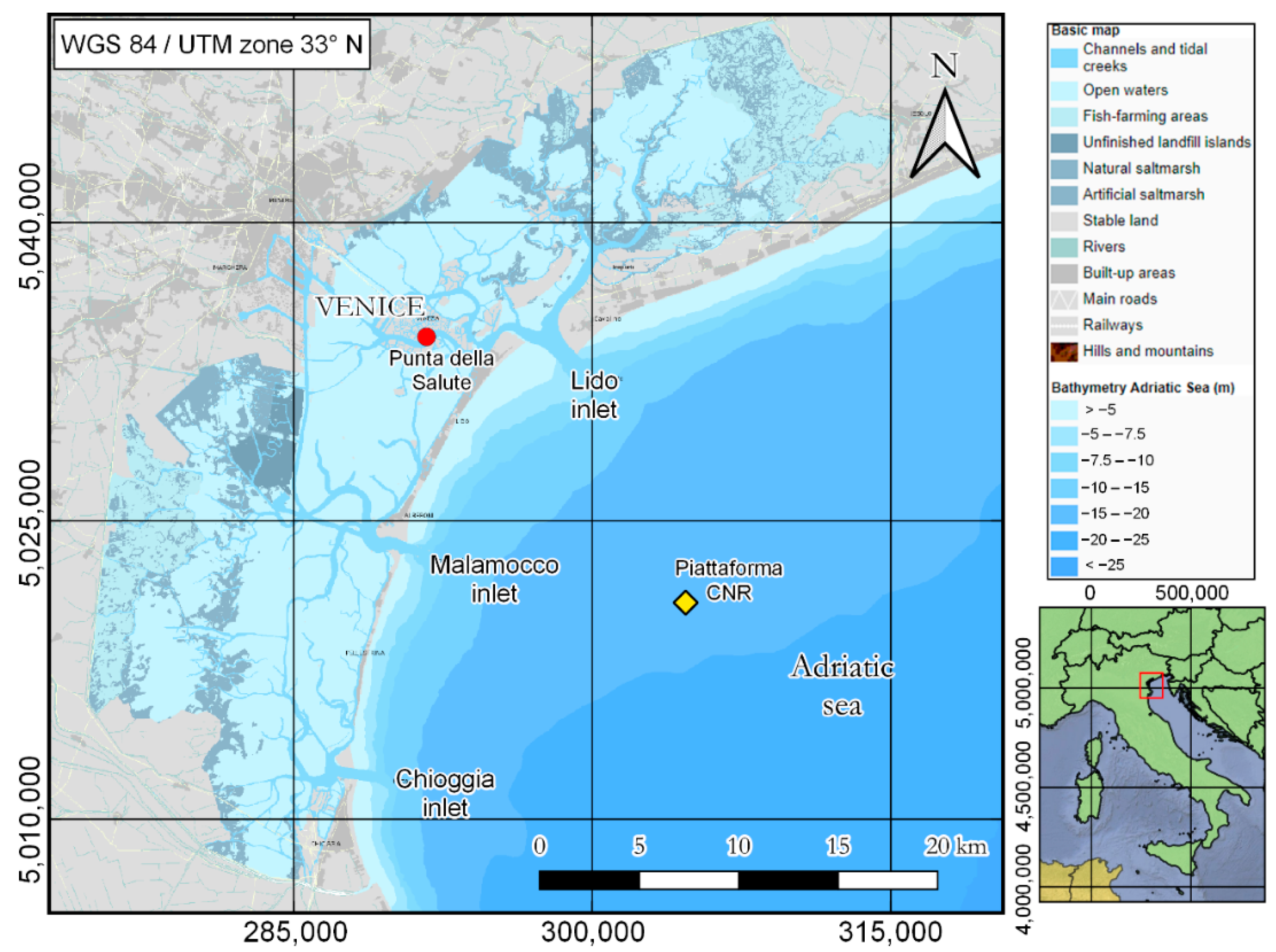
2.1. Study Area and Extreme Events

The Venice Lagoon is located in the Upper Adriatic and extends from the Sile river in the north to the Brenta river in the south, covering an area of 550 km². Only the 8% is represented by land, including the city of Venice and many smaller islands while about 11% is permanently covered by open water and 80% consists of mudflats, tidal shallows, and salt marshes. The lagoon is connected to the Adriatic Sea by means of three inlets: Lido, Malamocco, and Chioggia (Figure 1). In ordinary conditions, the observed sea level in the Lagoon is little different from that induced by the astronomical tide since meteorological effects are small. In the case of particularly adverse weather conditions, with significant drop pressure and strong sirocco wind, the meteorological effects become significant: if they are in phase with a high astronomical tide, they can lead to the phenomenon of high water, which is conventionally defined as a tide level greater than 80 cm with reference to the Punta della Salute tide gauge. At this tide level, the flooding of the lower part of the city begins. The storm surge may be enhanced by a severe low pressure on the upper Adriatic and contemporary high pressure on the lower Adriatic. The situation worsens further if a strong wind from North-East (Bora) blows in the northern Adriatic together with sirocco wind in middle Adriatic, leading to the convergence of wind-induced marine currents. In addition, due to the shape of the Adriatic Sea, a storm surge leads to the formation of seiches whose amplitude is progressively decreasing [25]. The concomitant action of the above factors can lead to extreme values of storm tide levels, as observed more and more frequently in recent decades.

The most well-known and impressive extreme event occurred on 4 November 1966. The storm tide level was the highest recorded, 194 cm [26]. The surge is even more impressive since the astronomical contribution to the observed peak was less than its mean level, so it was negative. Those days were characterized by exceptionally adverse weather conditions that caused extensive civil and hydrogeological damage in various areas of Italy, such as the famous flood in Florence. The sirocco wind was strong and persistent, reaching a speed of 52 knots in Venice, of 58 knots in lower Adriatic Sea. The pressure drop was 30 hPa in 2 days. The flood has been extremely long in time: the tide level persisted over 110 cm for 22 h.

Figure 1. Location of the Punta della Salute tide gauge ( ) and Piattaforma CNR weather station ( ), with a thematic map of the Venice Lagoon [27].

Figure 1. Location of the Punta della Salute tide gauge ( ) and Piattaforma CNR weather station ( ), with a thematic map of the Venice Lagoon [27].

The second most severe event of exceptional high water occurred in Venice on 12 November 2019 and resulted to the flooding of almost 90% of the city. In November 2019, there was an anomalous persistence of sirocco winds on the Adriatic Sea, which caused an accumulation of water masses in the Venetian Lagoon. The simultaneous persistence of low pressure on the upper Adriatic induced a significant rise in sea level, which was about 30 cm higher than the average value of the last 25 years.

In recent years, also due to eustatism and subsidence, as well as due to climate change, the extreme storm tide events affecting Venice have become increasingly frequent. The good availability of data relating to water level, wind characteristics, and barometric pressure has allowed to develop data-driven models capable of accurately predicting storm tide levels with forecast horizons of many hours. It is shown in the following that models based on NARX networks allow to predict even extreme events with high accuracy.

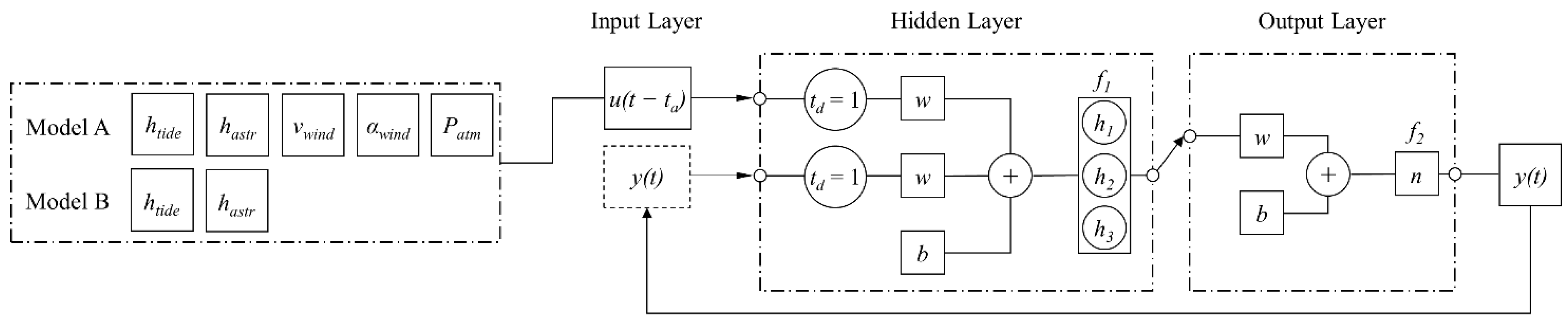
2.2. NARX Model Architectures

NARX is a recurrent dynamic network composed of interconnected nodes. Each node represents an artificial neuron that receives one or more inputs and elaborates them to produce an output. These sums pass through a non-linear activation function. The main advantages of the NARX networks with respect to other ANNs approaches are the faster convergence in reaching the optimal weights of the connections between neurons and input parameters [28] and the reduced number of the latter to calibrate and make the model effective [20]. The defining equation for the NARX model is:

$$y\left(t\right)=f\left(y\left(t-1\right),y\left(t-2\right),\dots ,y\left(t-n_y\right),u\left(t-1\right),u\left(t-2\right),\dots ,u\left(t-n_u\right)\right)$$

(1)

where u(t) and y(t) are, respectively, the input and output values at time t, n_u and n_y are the input and output network layers, and f is the non-linear function, approximating by the Feedforward Neural Network (FNN).

The NARX architectures include 3 different and sequential layers (Figure 2). The first is the input layer, which contains the input parameters of the neural network. The second is the hidden layer, which is the computational step between input and output. The third is the output layer, which leads to the predicted value y(t). Moreover, the output value is then fed back to the input values as part of the NARX architectures.

For the hidden layer, a sigmoid activation function f₁ was used, while a linear activation function f₂, with only one neuron n, was used for the output layer. A preliminary analysis was carried out to assess the optimal number of hidden nodes, which was found to be equal to 3 (Figure 2, indicated as h₁, h₂, and h₃). For the output layer, the weight w and bias b of the NARX model were optimized based on the Bayesian Regularization training algorithm. The NARX process was stopped if one of the following parameters was reached: the maximum number of epochs, settled equal to 1000; the Levenberg–Marquardt adjustment parameter, settled equal to 1 × 10⁻¹⁰; the error gradient was below a minimal value, settled equal to 1 × 10⁻⁷.

The Bayesian Regularization allows to achieve the best predictions in comparison with other two training algorithms preliminarily tested, the Levenberg–Marquardt and the Scaled Conjugate Gradient. It consists of a Gauss–Newton approximation to the Hessian matrix, based on the Bayesian technique proposed by MacKay (1992) [29], and implemented in the Levenberg–Marquardt algorithm, in order to reduce the probability of overfitting and the computational overhead [30]. Despite a slow convergence with respect to the direct application of Levenberg–Marquardt algorithm, the Bayesian Regularization algorithm usually leads to improved forecasting [22].

A normalization of the input values was also performed, in order to have a common range between 0 and 1 and improve the modeling performance. The water level, the astronomical tide, the barometric pressure and the wind speed were normalized with respect to the, respectively, maximum values along the time series, while the wind direction was divided by 360, equal to the complete angle in degree:

$$h_{tide,i}^{*}=\frac{h_{tide,i}}{\max \left(h_{tide}\right)}$$

(2)

$$h_{astr,i}^{*}=\frac{h_{astr,i}}{\max \left(h_{astr}\right)}$$

(3)

$$P_{atm,i}^{*}=\frac{P_{atm,i}}{\max \left(P_{atm}\right)}$$

(4)

$$v_{wind,i}^{*}=\frac{v_{wind,i}}{\max \left(v_{wind}\right)}$$

(5)

$${\alpha }_{wind,i}^{*}=\frac{{\alpha }_{wind,i}}{360}$$

(6)

where i indicates the temporal step and * indicates the dimensionless form of each parameter.

The two different NARX-based models were implemented in MATLAB^® 2020a environment [31]: Model A and Model B. The two models were different in the input variables. Both the models included the lagged values of the water level h_tide(t − t_a) among the inputs.

In addition, Model A considered astronomical tide h_astr(t − t_a), wind speed v_wind(t − t_a), wind direction α_wind(t − t_a), and barometric pressure P_atm(t − t_a) as exogenous input parameters, whereas Model B considered only h_astr(t − t_a) as an exogenous input variable. The astronomical tide h_astr(t − t_a) values were computed through the following:

$$h_{astr}=A_0+\sum _{n=1}^N{A}_n\cos \left({\sigma }_{n}t-k_n\right)$$

(7)

where A₀ is the average sea level, A_n is the amplitude, σ_n the angular frequency, k_n the phase delay of component n, and N is the number of harmonics used to evaluate the astronomical tide height. These values can be found on the Venice Municipality website [32].

It should be noted that, despite the meteorological parameters were neglected for Model B, their influence is implicitly expressed by including previously observed water level values, which in turn also depend on meteorological factors. Different lag time t_a values were considered, in order to assess the performance of the models as t_a increases: 12, 24, 48, and 72 h.

2.3. Evaluation Metrics

The performances of the NARX-based models were evaluated by means of three evaluation metrics: the coefficient of determination R², which assess how well the model replicates observed outcomes and predicts future outcomes, the Mean Absolute Error (MAE), which provides the average error magnitude for the predicted values, and the Relative Absolute Error (RAE), equal to the ratio between absolute error and absolute value of the difference between average and each measured values. These metrics are defined as:

$$R^2=1-\frac{{\sum }_{i=1}^m{\left(f_i-\overline{y_i}\right)}^2}{{\sum }_{i=1}^m{\left(\overline{y_a}-\overline{y_i}\right)}^2}$$

(8)

$$MAE=\frac{{\sum }_{i=1}^m\left|f_i-\overline{y_i}\right|}{m}$$

(9)

$$RAE=\frac{{\sum }_{i=1}^m\left|f_i-\overline{y_i}\right|}{{\sum }_{i=1}^m\left|\overline{y_a}-\overline{y_i}\right|}$$

(10)

where $m$ is the total number of measured data, $f_i$ is the predicted value for the i-th data, $\overline{y_i}$ is the measured value for the i-th data, and $\overline{y_a}$ is the averaged value of the measured data. The performances of the NARX-based model were computed considering only the extreme tidal events, with h_tide equal or greater than 110 cm.

3. Results and Discussion

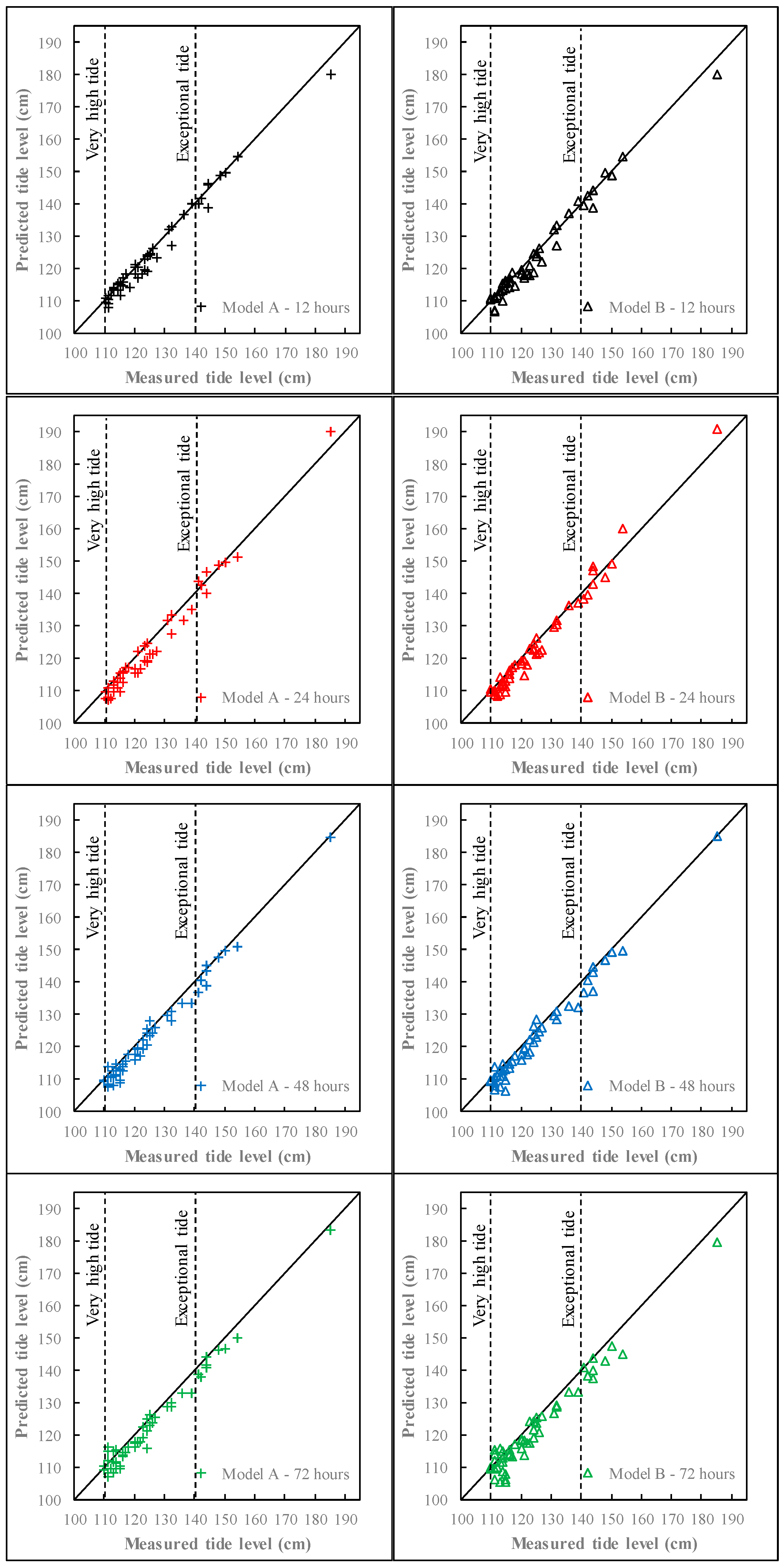
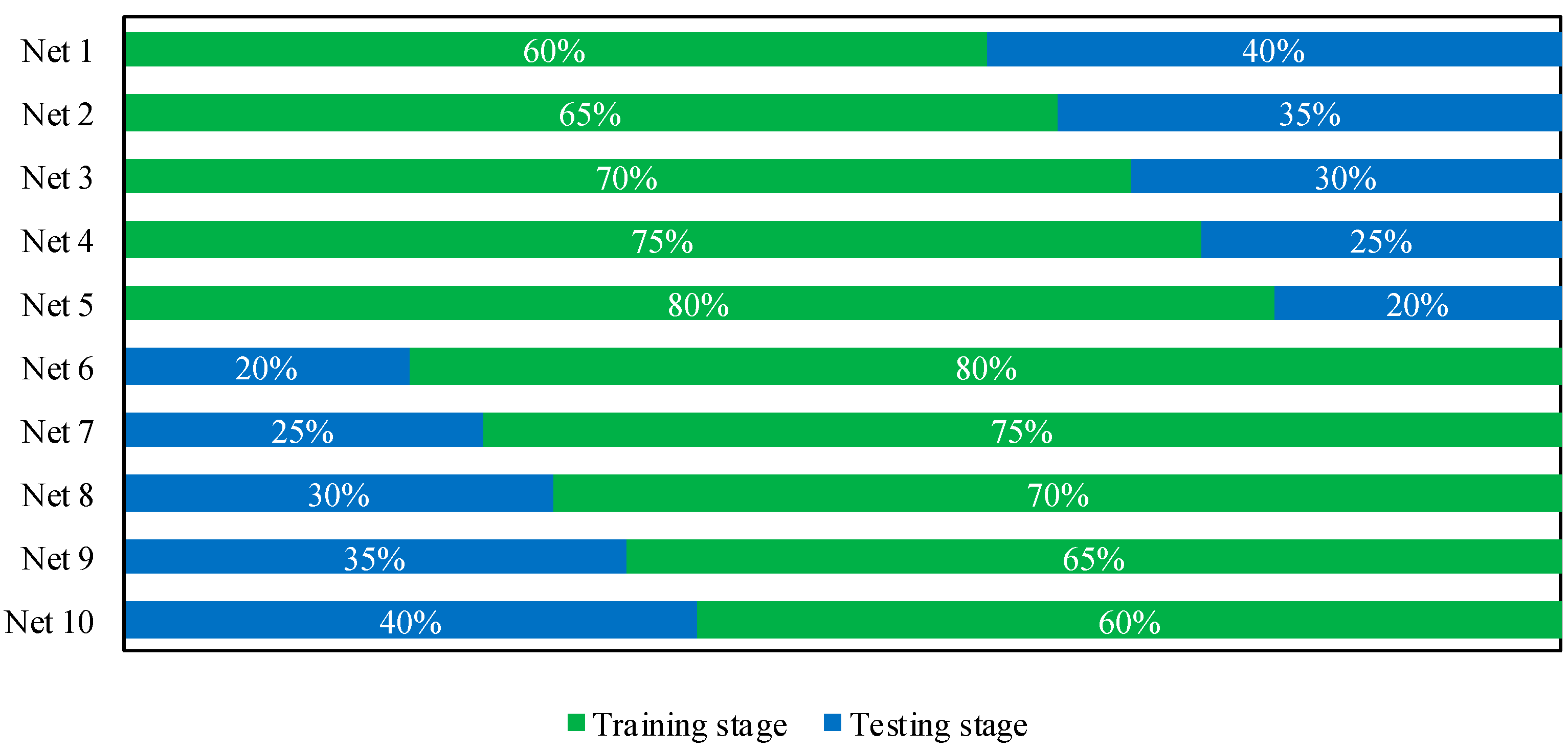
3.1. Training and Testing

The NARX-based models were trained using all water level data, collected between January 2009 and June 2012. After the training stage, the models were employed to simulate all the storm tide events characterized by a level higher than 110 cm that occurred from January 2009 to December 2020. Overall, 52 extreme storm tide events were identified. Of these, 43 events are classified as very high storm tide, with sea level between 110 cm and 140 cm, and 9 events as exceptional storm tide, with storm tide higher than 140 cm.

The NARX-based model showed a very good fit for both Model A and Model B and for all lag time (

Table 1. Forecasting performance.

Metric	Model A				Model B
	ta = 12 h	ta = 24 h	ta = 48 h	ta = 72 h	ta = 12 h	ta = 24 h	ta = 48 h	ta = 72 h
R2	0.950	0.923	0.911	0.899	0.941	0.905	0.888	0.860
MAE (cm)	1.96	2.46	2.91	2.91	2.14	2.55	3.05	3.29
RAE (%)	23.03	28.95	34.21	34.25	25.13	29.97	35.87	38.75

). The best results were achieved for the lower t_a, equal to 12 h (Model A—R² = 0.950, MAE = 1.96 cm and RAE = 23.03%; Model B—R² = 0.941, MAE = 2.14 cm, and RAE = 25.13%). The prediction performance reduces as the lag time increases, with the NARX models providing the less accurate forecasts for t_a = 72 h (Model A—R² = 0.899, MAE = 2.91 cm, and RAE = 34.25%; Model B—R² = 0.860, MAE = 3.29 cm, and RAE = 38.75%). In Figure 3 the comparison between measured and predicted extreme storm tide levels for both Model A and Model B, and for different lag times is reported, highlighting a slight tendency to underestimate these extreme events. Overall, regardless of the lag time, the NARX network-based models are able to forecast extreme storm tide events, including the exceptional storm tides. Moreover, the model performance was not significantly affected by the additional input parameters: Model B is only slightly less accurate than model A. This obviously does not mean that the weather parameters have little influence on extreme events: the fundamental influence of the weather parameters is taken into account by means of the lagged values of the storm tide level [24].

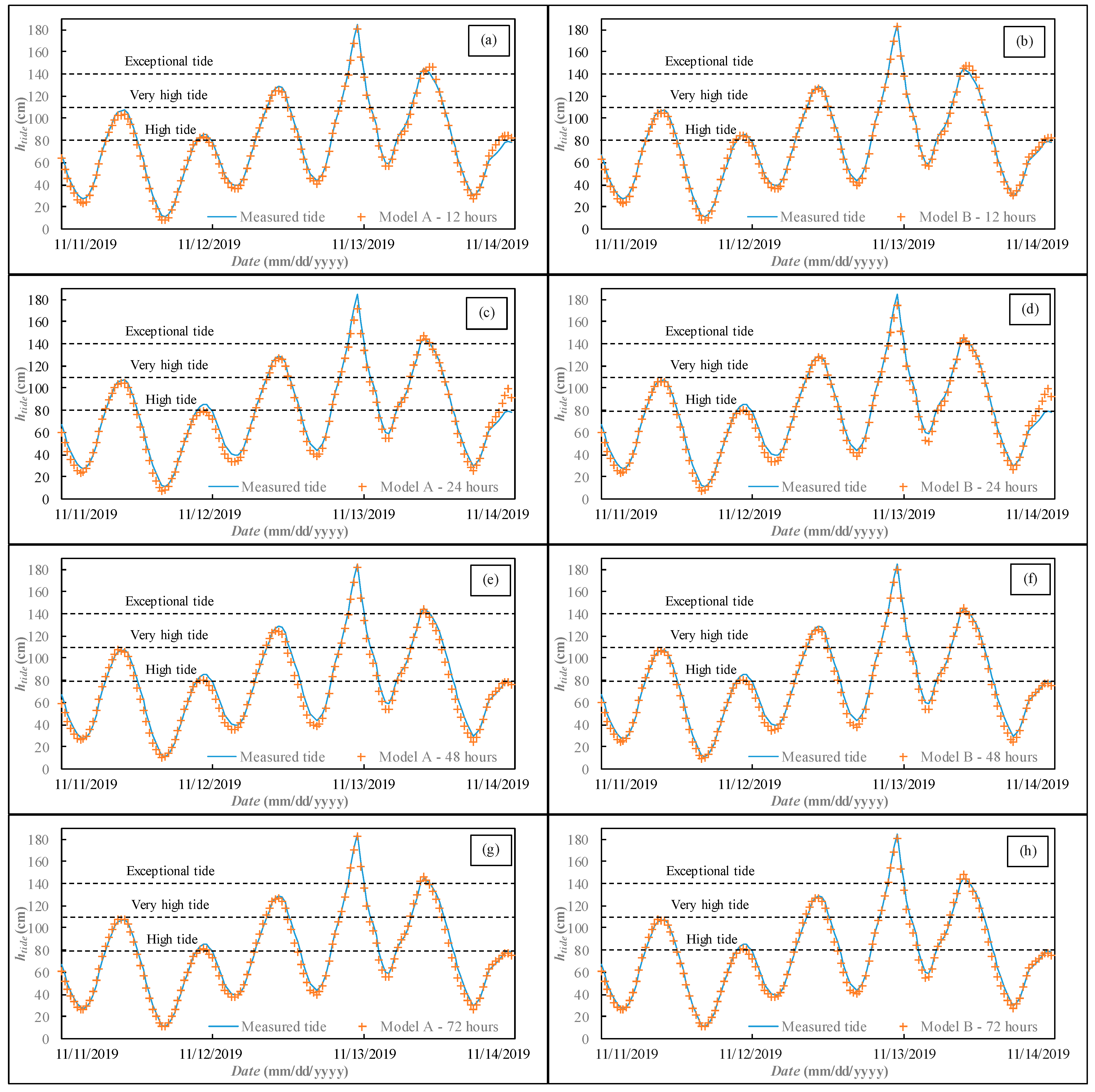
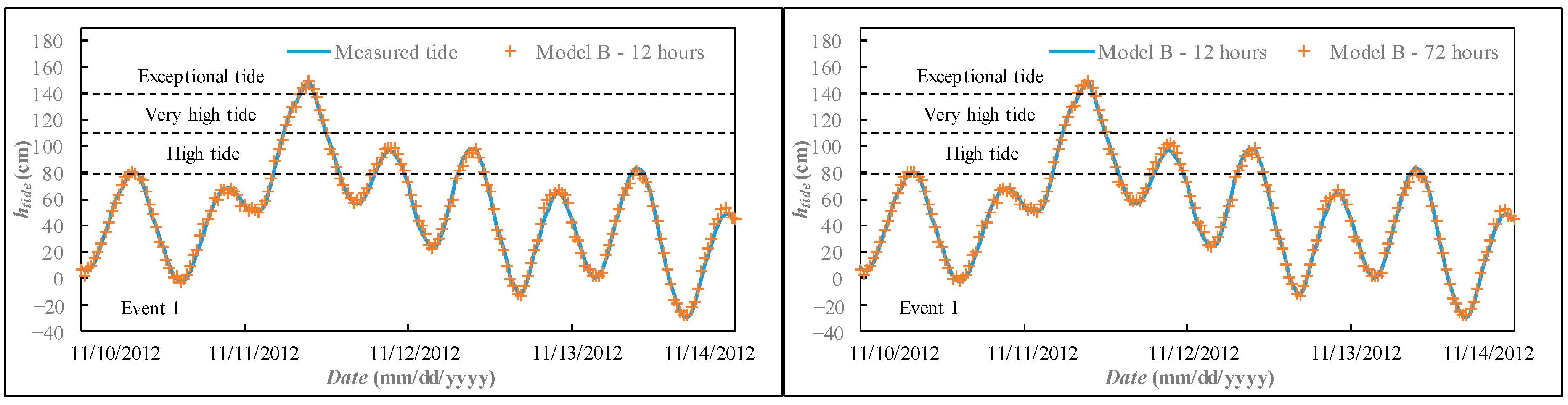
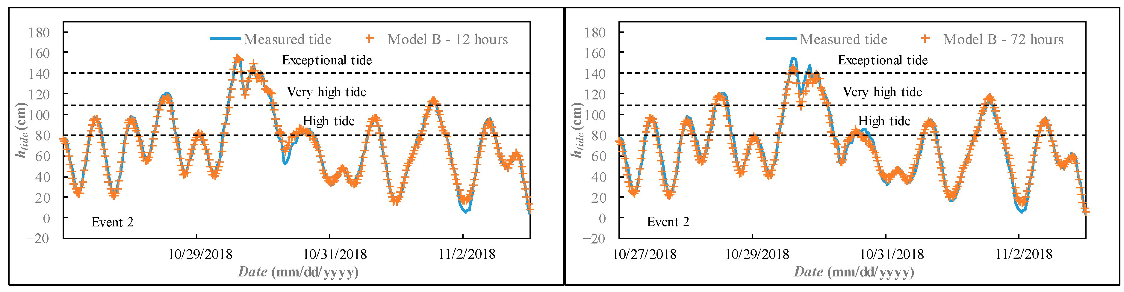
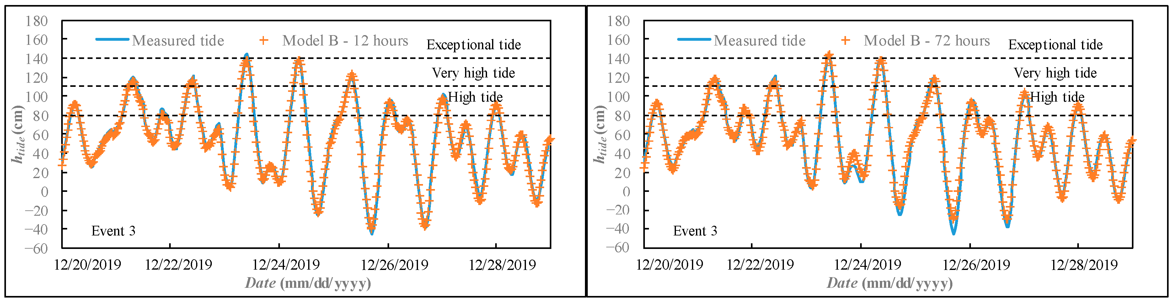
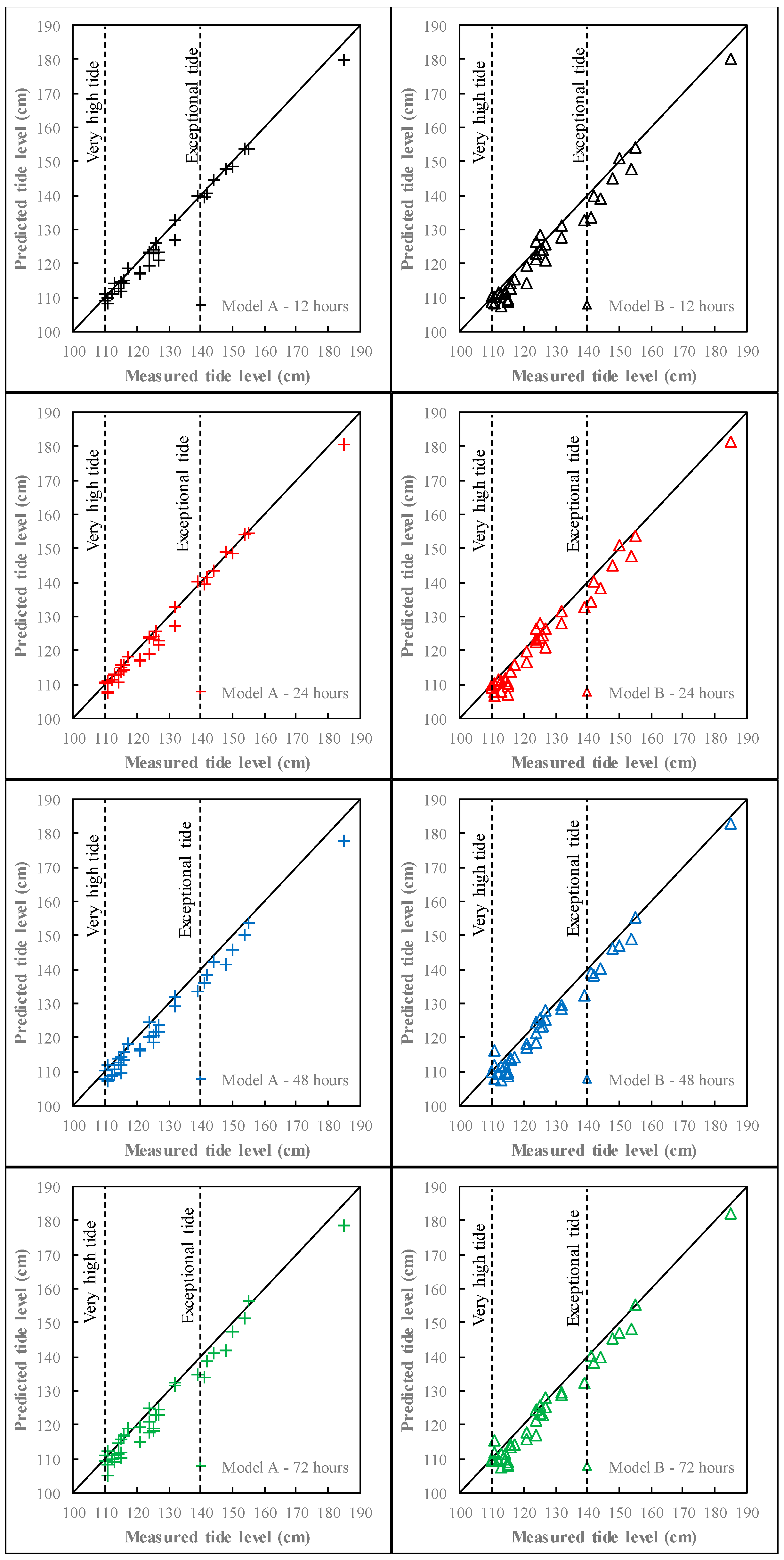
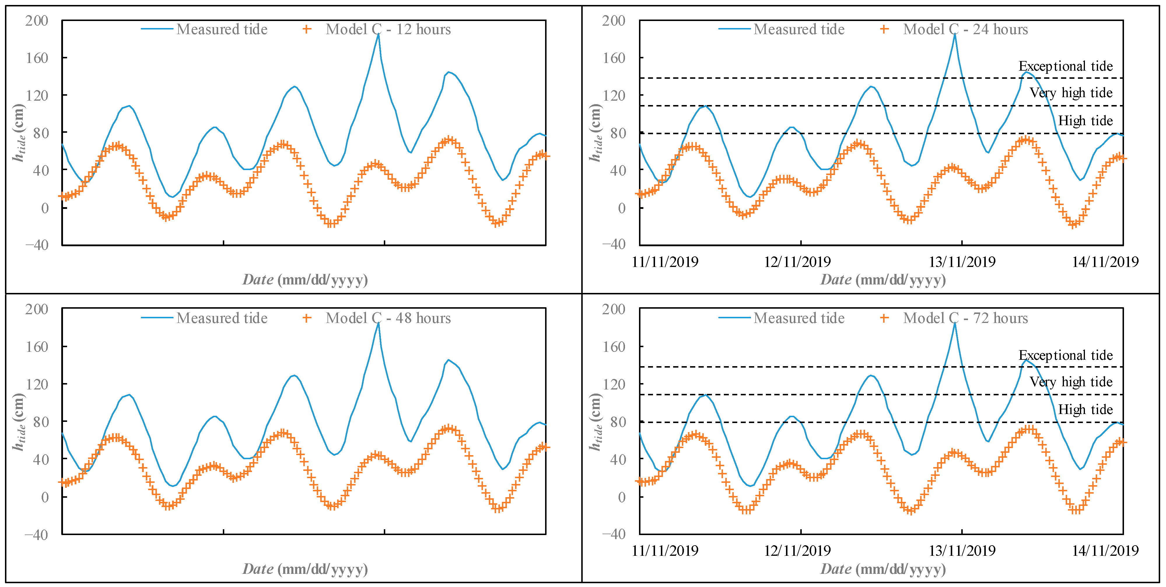
3.2. Time Series Analysis

A further analysis was carried out on the time series related to the extreme storm tide events, in order to evaluate the ability of NARX to provide reliable predictions in the hours before and after the water level peaks, but also the sea level during the whole storm tide event. As an example, the modeling of the highest storm tide in the entire investigated period, equal to 185 cm, is here described. This event took place from 11 to 14 November 2019. Marked level fluctuations, with five peaks, were observed, passing from a minimum sea level of 11 cm on 11 November 2019 to the highest peak of 185 cm on 12 November 2019, with intermediate peaks equal to 108, 85, 129, and 145 cm, classifiable, respectively, as high storm tide (between 80 and 110 cm), very high storm tide, and exceptional storm tide.

For both Model A and Model B, and for all the tested lag times, the NARX network has proven to be able to forecast that extreme event by accurately simulating the storm tide trend. For the 85 cm peak, Model A provides the best prediction with the lower t_a, equal to 12 h, with an overestimation of the storm tide equal to 0.29 cm. Model B also provides very good outcomes: the less accurate forecast was obtained for t_a = 24 h, with an underestimation of 3.08 cm. For the third peak, equal to 129 cm, a very effective prediction was achieved with Model A also for t_a = 72 h, with a slight underestimation of just 0.02 cm. For the same lag time, Model B provides a very accurate forecast too, with an underestimation of 0.61 cm. For the exceptional tide peak = 185 cm, the best forecast was achieved with Model A and t_a = 48 h, with an underestimation of 0.2 cm. However, Model B also provided accurate predictions for all lag times, and the worst forecast was obtained for t_a = 24 h, with an overestimation of 5.99 cm. Following this peak, there is a further exceptional storm tide, corresponding to a 145 cm sea level, the last of the considered period. For the latter, the best forecasts were again achieved with Model A, with an underestimation of 0.27 cm for t_a = 24 h. However, accurate predictions were also obtained with Model B, with an underestimation of 0.28 cm in the case of t_a = 48 h.

Figure 4 reports the comparison between measured and predicted sea level for both Model A and Model B and for the different lag times.

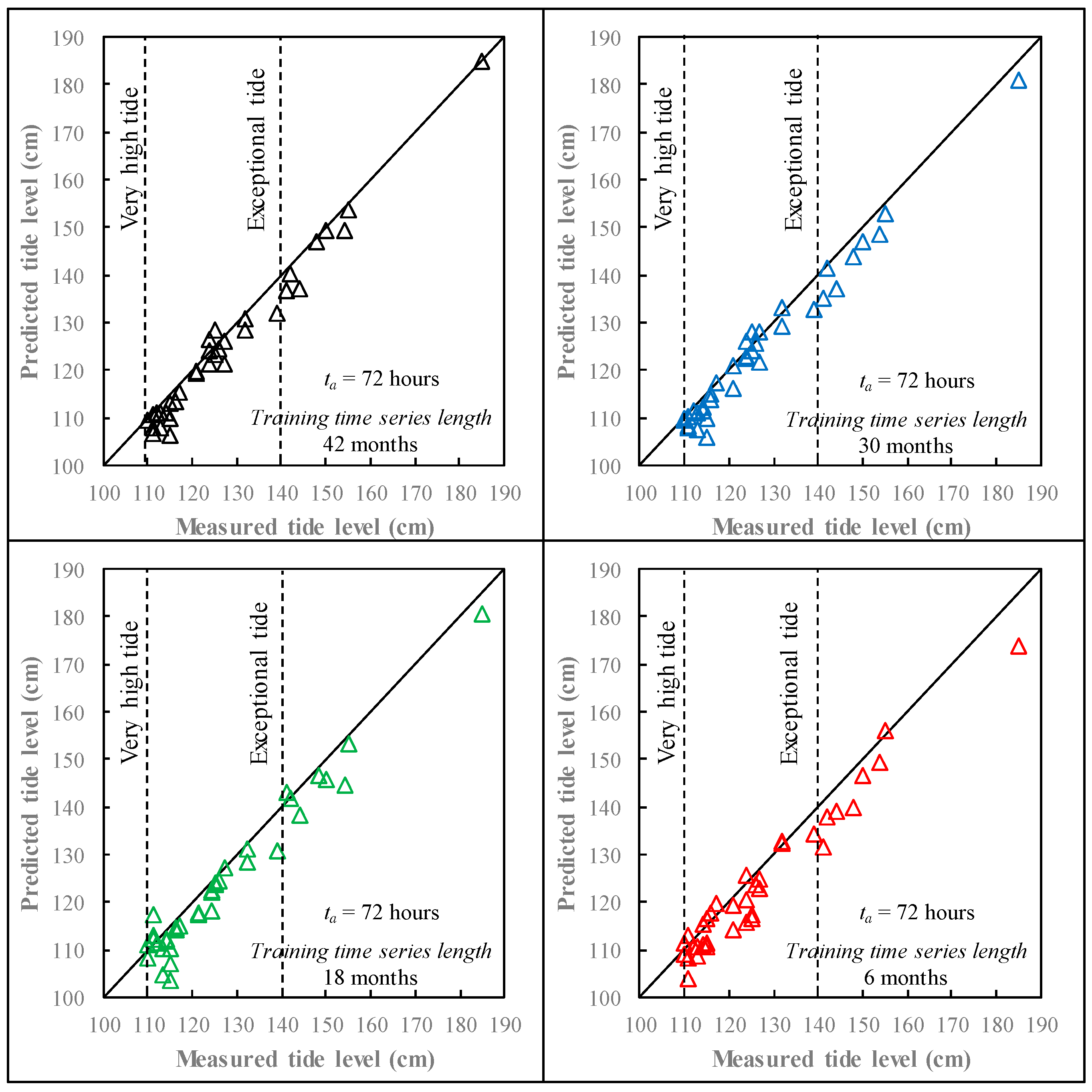
3.3. Sensitivity Analysis

The sensitivity of the NARX-based models to the training time series length and to the duration of the extreme tidal events is discussed in this section.

Model B was considered to assess the prediction accuracy as the training time series length decreases. A total of four different training time series lengths were investigated: overall, 42 months (from January 2009 to June 2012), corresponding to the full length time series (which has been already considered in Section 3.1), 30 months (from January 2010 to June 2012), 18 months (from January 2011 to June 2012), and 6 months (from January 2012 to June 2012).

Figure 5 provides a comparison between measured and predicted tide for a lag time equal to 72 h, which is the most challenging case. The best predictions were obtained for the full length training time series (R² = 0.860, MAE = 3.29 cm, and RAE = 38.75%). As expected, a performance reduction was observed as the length of the time series reduced (

Table 2. Forecasting performance—Sensitivity analysis to the training time series length.

Time Series Length for the Training	ta (h)	R2	MAE (cm)	RAE (%)
January 2009–June 2012 (Full length)	12	0.941	2.14	25.13
	24	0.905	2.55	29.97
	48	0.888	3.05	35.87
	72	0.860	3.29	38.75
January 2010–June 2012	12	0.937	2.19	25.25
	24	0.905	3.14	33.66
	48	0.869	3.18	36.16
	72	0.844	3.43	39.12
January 2011–June 2012	12	0.924	2.61	26.14
	24	0.898	3.25	35.72
	48	0.863	3.23	38.03
	72	0.832	3.56	40.06
January 2012–June 2012	12	0.902	2.67	30.04
	24	0.891	3.54	37.12
	48	0.844	3.71	38.36
	72	0.820	3.96	40.57

), with the worst predictions obtained with the shorter training time series (R² = 0.820, MAE = 3.96 cm, and RAE = 40.57%).

However, predictions obtained even with a reduced time series length were still quite accurate.

The prediction accuracy for extreme tidal events with different duration was evaluated considering three different events.

Figure 6 reports the comparison between measured and predicted tide for an extreme storm tidal event that occurred between 10 November 2012 and 14 November 2012 (indicated as Event 1), with a duration of 48 h. An exceptional storm tide was recorded during this event, with h_tide higher than 140 cm. As confirmed by the metrics, reported in

Table 3. Forecasting performance—Events: 1, 2 and 3.

Event	Metric	Model A				Model B
		ta = 12 h	ta = 24 h	ta = 48 h	ta = 72 h	ta = 12 h	ta = 24 h	ta = 48 h	ta = 72 h
Event 1 (length 48 h)	R2	0.995	0.993	0.990	0.989	0.995	0.989	0.989	0.975
	MAE (cm)	2.01	2.66	3.35	3.56	2.04	3.53	3.44	4.68
	RAE (%)	6.59	8.71	10.99	11.68	6.69	11.58	11.28	15.33
Event 2 (length 168 h)	R2	0.992	0.989	0.987	0.984	0.987	0.982	0.975	0.974
	MAE (cm)	2.43	2.70	3.24	3.53	2.76	3.65	4.17	4.09
	RAE (%)	9.30	10.33	12.37	13.49	10.57	13.96	15.95	15.62
Event 3 (length 216 h)	R2	0.995	0.993	0.992	0.992	0.992	0.988	0.988	0.986
	MAE (cm)	2.46	2.85	2.75	2.95	2.90	3.26	3.46	3.30
	RAE (%)	7.88	9.13	8.80	9.44	9.28	10.42	11.07	10.54

, both models A and B were able to provide accurate predictions of this event, for all lag times.

Figure 7 reports a second event (Event 2) which occurred between 27 October 2018 and 3 November 2018, with a duration of 168 h. The two consecutive exceptional storm tides were measured during this period, with also two very high storm tides (h_tide higher than 110 cm) before and after the exceptional storm tides. Additionally, in this case, predictions were very accurate, with a slight underestimation of the exceptional storm tides for Model B and t_a = 72 h.

The third event (Event 3) is shown in Figure 8. It occurs between 20 December 2019 and 29 December 2019, with a duration of 216 h. During this period, one exceptional storm tide was measured, preceded by two very high storm tides, and followed by another very high storm tide. In this case, it is observed that both Model A and Model B are able to provide an accurate prediction of the peaks, for all lag times.

The analysis of the investigated events indicates that the accuracy of the model is not affected by the duration of the storm tide event (Table 3).

3.4. Comparison with Other Models

The accuracy of NARX-based models in predicting extreme events was compared with that of two statistical models, referred as ISPRA statistical models (ISPRA-STAT2008 [33]), and one deterministic model, referred as Shallow water Hydrodynamic Finite Element Model (SHYFEM [4,34]).

To evaluate the prediction accuracy of the deterministic model, the results of a modeling carried out in the period 1 October 2012–1 October 2013 for the tide gauge of Punta della Salute were considered. The evaluation of the prediction accuracy for the statistical models was instead carried out for the period 18 March 2012–30 June 2013 for the same tide gauge [35]. The comparison was conducted based on an accuracy index, expressed as:

$$I={\epsilon }_m\pm 2\sigma$$

(11)

where ε_m indicates the mean error and 2σ the confidence interval, with σ representing the standard deviation of the errors, i.e., the differences between predicted and measured levels.

Statistical models take into account the hourly time series of the sea level and of the meteorological parameters, such as barometric pressure, wind speed, and wind direction observed in the previous hours. For the first model, referred as STAT-1, the meteorological parameters were provided by the European center ECMWF, while for the second model, referred as STAT-2, those parameters were provided by the BOLAM limited area hydrostatic model [36]. The SHYFEM model consists of a two-dimensional hydrodynamic model which allows to forecast the sea level over the entire Mediterranean basin, based on the wind speed, wind direction, and atmospheric pressure fields provided both by ECMWF (SHYFEM 5) and BOLAM (SHYFEM 6), as for the statistical models [37].

Table 4. Accuracy index grouping the measured tides by height classes: comparison between NARX, SHYFEM, and statistical models.

htide (cm)	ta (h)	I = εm + 2σ (cm)				STAT-1	STAT-2
		Model A	Model B	SHYFEM 5	SHYFEM 6
80–100	24	−1.2 ± 5.5	−1.4 ± 6.1	2.0 ± 12.9	1.0 ± 16.8	−3.7 ± 16.1	−4.0 ± 16.6
	48	−1.1 ± 6.3	−1.1 ± 6.4	1.6 ± 18.3	−0.6 ± 18.7
	72	−0.9 ± 6.1	−0.9 ± 6.2	1.9 ± 18.5	−0.3 ± 20.9
101–120	24	−1.6 ± 5.5	−1.6 ± 5.4	0.5 ± 12.5	−3.6 ± 19.6	−5.7 ± 20.7	−5.3 ± 23.3
	48	−1.8 ± 5.9	−1.9 ± 6.1	−3.1 ± 17.5	−5.5 ± 24.8
	72	−1.5 ± 5.8	−1.6 ± 6.6	−2.8 ± 20.6	−6.8 ± 26.4
>120	24	−1.5 ± 5.1	−1.1 ± 5.3	−9.4 ± 26.2	−0.0 ± 26.1	−19.4 ± 27.0	−16.7 ± 26.2
	48	−2.2 ± 5.1	−2.5 ± 6.9	−8.6 ± 21.2	0.2 ± 14.8
	72	−2.0 ± 5.2	−2.7 ± 7.0	−11.1 ± 16.8	−8.8 ± 47.0

reports the values of the accuracy index, showing a comparison between NARX-based models, SHYFEM, and statistical models, and grouping the measured levels in height classes. As for the statistical models, the comparison was made regardless of the lag times, while for the SHYFEM model data relating to lag times equal to 24, 48, and 72 h were available.

For h_tide in the range of 80 to 100 cm, SHYFEM model highlights mean errors which, for t_a = 72 h, reach values closer to 0 with respect to the NARX models (Model A—ε_m = −0.9 cm, SHYFEM 6—ε_m = −0.3 cm). However, both NARX-based models exhibit significantly narrower confidence interval 2σ in comparison with SHYFEM and statistical models. In particular, for h_tide between 80 and 100 cm, the lower value of 2σ was computed for Model A and t_a = 24 h, equal to 5.5 cm (Model B and t_a = 24 h—2σ = 6.1 cm). Considering the same h_tide interval and lag time, deterministic and statistical models shows a wider confidence interval, with 2σ equal to 12.9, 16.8, 16.1, and 16.6 cm, respectively, for SHYFEM 5, SHYFEM 6, STAT-1, and STAT-2. Moreover, NARX models do not show a marked increase in 2σ as the lag time increases, with 2σ = 6.1 cm for Model A and t_a = 72 h (Model B and t_a = 72 h—2σ = 6.2 cm). The same cannot be said for the deterministic models that highlight a relevant increase in 2σ as the lag time increases, with 2σ equal to 18.5 cm (SHYFEM 5) and 20.9 cm (SHYFEM 6) for t_a = 72 h.

As the storm tide level increases, statistical models exhibit a marked widening of the confidence interval. In particular, for h_tide > 120 cm, STAT-1 and STAT-2 show 2σ values, respectively, equal to 27 and 26.2 cm. Even the deterministic models exhibit a widening of the confidence interval. For t_a = 24 h, 2σ equal to 26.2 and 26.1 cm were, respectively, computed for SHYFEM 5 and SHYFEM 6. As the lag time increases, instead, SHYFEM 5 and SHYFEM 6 show an opposite trend, with a narrowing of the confidence interval for the first model (2σ = 16.8 cm) and a widening of the same for the second model (2σ = 47.0 cm). NARX-based models instead are characterized by confidence intervals similar to those computed for h_tide between 80 and 100 cm. As for Model A, 2σ values were equal to 5.1 and 5.2 cm, respectively, for lag times of 24 and 72 h. Model B shows a greater widening of the confidence interval as the lag time increases, passing from 5.3 cm for t_a = 24 h to 7 cm for t_a = 72 h.

Overall, the NARX-based models highlight good accuracy for all lag times (from this point of view, the NARX-based models would seem to outperform those based on different Machine Learning algorithms, such as M5P and RF [38]) and sea level with a narrow confidence interval in comparison with the statistical and deterministic models, confirming the ability of the NARX network to provide reliable predictions of extreme storm tide events.

4. Conclusions

This study assessed the ability of NARX network-based models to forecast extreme storm tide events in Venice. A total of two models were built, including the lagged values of the measured sea level and astronomical tide as input values. In the first one, Model A, also the meteorological parameters related to wind features and barometric pressure were taken into account. The prediction accuracy of this model was very good. Meteorological parameters are not included as input in Model B, however, their influence is implicitly expressed by previously observed sea level values, leading to a still high prediction accuracy.

The ability to forecast even the exceptional storm tides, linked with a narrow confidence interval compared to different statistical and deterministic models, makes the NARX networks a reliable tool for the extreme storm tide events forecasting in Venice. Moreover, the limited effect of the lag time increase on the forecasting performance demonstrates the great capability of NARX networks to predict extreme events with a forecasting horizon of 1–3 days, that allows a timely activation of the MOSE barriers.

However, it should be noted that such an approach leads to satisfactory results in appropriately monitored sites, for which adequate datasets are available, including even extreme events. Therefore, where sufficient data are not available, with particular reference to extreme events, an approach based on Machine Learning algorithms cannot be used.

References

1. Garrett, C. Tidal resonance in the Bay of Fundy and Gulf of Maine. Nature 1972, 238, 441–443. [Google Scholar] [CrossRef]
2. Andersen, C.F.; Battjes, J.A.; Daniel, D.E.; Edge, B.; Espey, W., Jr.; Gilbert, R.B.; Jackson, T.L.; Kennedy, D.; Mileti, D.S.; Mitchell, J.K.; et al. The New Orleans Hurricane Protection System: What Went Wrong and Why (Report); American Society of Civil Engineers: Reston, VA, USA, 2007. [Google Scholar]
3. Tosoni, A.; Canestrelli, P. Il modello stocastico per la previsione di marea a Venezia. Atti Ist. Veneto Sci. Lett. Arti. 2011, 169, 2010–2011. [Google Scholar]
4. Umgiesser, G.; Canu, D.M.; Cucco, A. A finite element model for the Venice Lagoon. Development, set up, calibration and validation. J. Mar. Syst. 2004, 51, 123–145. [Google Scholar] [CrossRef]
5. Kişi, Ö. Streamflow forecasting using different artificial neural network algorithms. J. Hydrol. Eng. 2007, 12, 532–539. [Google Scholar] [CrossRef]
6. Wang, W.C.; Chau, K.W.; Cheng, C.T.; Qiu, L. A comparison of performance of several artificial intelligence methods for forecasting monthly discharge time series. J. Hydrol. 2009, 374, 294–306. [Google Scholar] [CrossRef] [Green Version]
7. Granata, F.; Gargano, R.; De Marinis, G. Support vector regression for rainfall-runoff modeling in urban drainage: A comparison with the EPA’s storm water management model. Water 2016, 8, 69. [Google Scholar] [CrossRef]
8. Yaseen, Z.M.; Jaafar, O.; Deo, R.C.; Kisi, O.; Adamowski, J.; Quilty, J.; El-Shafie, A. Stream-flow forecasting using extreme learning machines: A case study in a semi-arid region in Iraq. J. Hydrol. 2016, 542, 603–614. [Google Scholar] [CrossRef]
9. Granata, F.; Saroli, M.; de Marinis, G.; Gargano, R. Machine learning models for spring discharge forecasting. Geofluids 2018, 2018, 8328167. [Google Scholar] [CrossRef] [Green Version]
10. Mouatadid, S.; Raj, N.; Deo, R.C.; Adamowski, J.F. Input selection and data-driven model performance optimization to predict the Standardized Precipitation and Evaporation Index in a drought-prone region. Atmos. Res. 2018, 212, 130–149. [Google Scholar] [CrossRef]
11. Granata, F. Evapotranspiration evaluation models based on machine learning algorithms—A comparative study. Agric. Water Manag. 2019, 217, 303–315. [Google Scholar] [CrossRef]
12. Granata, F.; Gargano, R.; de Marinis, G. Artificial intelligence based approaches to evaluate actual evapotranspiration in wetlands. Sci. Total Environ. 2020, 703, 135653. [Google Scholar] [CrossRef]
13. Imani, M.; Kao, H.C.; Lan, W.H.; Kuo, C.Y. Daily sea level prediction at Chiayi coast, Taiwan using extreme learning machine and relevance vector machine. Glob. Planet. Chang. 2018, 161, 211–221. [Google Scholar] [CrossRef]
14. Liu, J.; Shi, G.; Zhu, K. High-Precision Combined Tidal Forecasting Model. Algorithms 2019, 12, 65. [Google Scholar] [CrossRef] [Green Version]
15. Jain, P.; Deo, M.C. Real-time wave forecasts off the western Indian coast. Appl. Ocean Res. 2007, 29, 72–79. [Google Scholar] [CrossRef]
16. Karimi, S.; Kisi, O.; Shiri, J.; Makarynskyy, O. Neuro-fuzzy and neural network techniques for forecasting sea level in Darwin Harbor, Australia. Comput. Geosci. 2013, 52, 50–59. [Google Scholar] [CrossRef]
17. Riazi, A. Accurate tide level estimation: A deep learning approach. Ocean Eng. 2020, 198, 107013. [Google Scholar] [CrossRef]
18. Yang, S.; Yang, D.; Chen, J.; Zhao, B. Real-time reservoir operation using recurrent neural networks and inflow forecast from a distributed hydrological model. J. Hydrol. 2019, 579, 124229. [Google Scholar] [CrossRef]
19. Lee, W.K.; Resdi, T.A. Simultaneous hydrological prediction at multiple gauging stations using the NARX network for Kemaman catchment, Terengganu, Malaysia. Hydrol. Sci. J. 2016, 61, 2930–2945. [Google Scholar] [CrossRef] [Green Version]
20. Guzman, S.M.; Paz, J.O.; Tagert, M.L.M. The Use of NARX Neural Networks to Forecast Daily Groundwater Levels. Water Resour. Manag. 2017, 31, 1591–1603. [Google Scholar] [CrossRef]
21. Rjeily, Y.A.; Abbas, O.; Sadek, M.; Shahrour, I.; Chehade, F.H. Flood forecasting within urban drainage systems using NARX neural network. Water Sci. Technol. 2017, 76, 2401–2412. [Google Scholar] [CrossRef] [PubMed]
22. Di Nunno, F.; Granata, F. Groundwater level prediction in Apulia region (Southern Italy) using NARX neural network. Environ. Res. 2020, 190, 110062. [Google Scholar] [CrossRef]
23. Siegelmann, H.T.; Horne, B.G.; Giles, C.L. Computational capabilities of recurrent NARX neural networks. IEEE Trans. Syst. Man. Cybern. B Cybern. 1997, 27, 208–215. [Google Scholar] [CrossRef] [PubMed] [Green Version]
24. Di Nunno, F.; de Marinis, G.; Gargano, R.; Granata, F. Tide prediction in the Venice Lagoon using Nonlinear Autoregressive Exogenous (NARX) neural network. Water 2021. under review. [Google Scholar]
25. Franco, P.; Jeftic, L.; Rizzoli, P.M.; Michelato, A.; Orlic, M. Descriptive model of the northern Adriatic. Oceanol. Acta 1982, 5, 379–389. [Google Scholar]
26. Zolt, S.D.; Lionello, P.; Nuhu, A.; Tomasin, A. The disastrous storm of 4 November 1966 on Italy. Nat. Hazards Earth Sys. 2006, 6, 861–879. [Google Scholar] [CrossRef] [Green Version]
27. Atlas of the Lagoon. Basic Map. 2020. Available online: http://atlante.silvenezia.it/en/index_ns.html (accessed on 14 April 2021).
28. Desouky, M.M.A.; Abdelkhalik, O. Wave prediction using wave rider position measurements and NARX network in wave energy conversion. Appl. Ocean Res. 2019, 82, 10–21. [Google Scholar] [CrossRef]
29. MacKay, D.J.C. Bayesian Interpolation. Neural Comput. 1992, 4, 415–447. [Google Scholar] [CrossRef]
30. Foresee, F.D.; Hagan, M.T. Gauss-Newton approximation to Bayesian learning. In Proceedings of the International Conference on Neural Networks (ICNN’97), Houston, TX, USA, 12 June 1997; Volume 3, pp. 1930–1935. [Google Scholar] [CrossRef]
31. MathWorks. MATLAB Deep Learning Toolbox Release 2020a; MathWorks: Natick, MA, USA, 2020. [Google Scholar]
32. Comune di Venezia. Centro Previsioni e Segnalazioni Maree La marea La marea astronomica. 2020. Available online: https://www.comune.venezia.it/it/content/la-marea-astronomica (accessed on 14 April 2021).
33. ARPA. Operational Oceanography in Italy toward a Sustainable Management of the Sea; Oddo, P., Coppini, G., Sorgente, R., Cardin, V., Reseghetti, F., Eds.; Arpa Emilia-Romagna: Bologna, Italy, 2012; Available online: https://www.arpae.it/it/documenti/pubblicazioni/quaderni/oceanografia-operativa-in-italia-operational-oceanography-in-italy (accessed on 14 April 2021).
34. Umgiesser, G. The impact of operating the mobile barriers in Venice (MOSE) under climate change. J. Nat. Conserv. 2020, 54, 125783. [Google Scholar] [CrossRef]
35. ISPRA. Modellistica Accuratezza dei Modelli. 2020. Available online: https://www.venezia.isprambiente.it/modellistica#Accuratezza%20dei%20modelli (accessed on 14 April 2021).
36. Mariani, S.; Casaioli, M.; Coraci, E.; Malguzzi, P. A new high-resolution BOLAM-MOLOCH suite for the SIMM forecasting system: Assessment over two HyMeX intense observation periods. Nat. Hazards Earth Syst. Sci. 2015, 15, 1–24. [Google Scholar] [CrossRef] [Green Version]
37. CNR-ISMAR. Shallow Water Hydrodynamic Finite Element Model SHYFEM. 2020. Available online: https://sites.google.com/site/shyfem (accessed on 14 April 2021).
38. Granata, F.; Di Nunno, F. Artificial Intelligence models for prediction of the tide level in Venice. Stoch. Environ. Res. Risk Assess. 2021, 1–12. [Google Scholar] [CrossRef]
Figure 2. Sketch of the NARX model architecture.
Atmosphere 12 00512 g002
Figure 3. Comparison between measured and predicted storm tide.
Atmosphere 12 00512 g003
Figure 4. Extreme storm tide events forecasting in the period 11–14 November 2019, comparison between measured time series and predicted values: Model A—ta = 12 h (a); Model B—ta = 12 h (b); Model A—ta = 24 h (c); Model B—ta = 24 h (d); Model A—ta = 48 h (e); Model B—ta = 48 h (f); Model A—ta = 72 h (g); Model B—ta = 72 h (h).
Atmosphere 12 00512 g004
Figure 5. Comparison between measured and predicted storm tide—Sensitivity analysis to the training time series length.
Atmosphere 12 00512 g005
Figure 6. Event 1, extreme storm tide event forecasting for the period 10–14 November 2012, comparison between measured time series and predicted values: Model B, ta = 12 h (on the left), ta = 72 h (on the right).
Atmosphere 12 00512 g006
Figure 7. Event 2, extreme storm tide event forecasting for the period 27 October–3 November 2018, comparison between measured time series and predicted values: Model B, ta = 12 h (on the left), ta = 72 h (on the right).
Atmosphere 12 00512 g007
Figure 8. Event 3, extreme storm tide event forecasting for the period 20–29 December 2019, comparison between measured time series and predicted values: Model B, ta = 12 h (on the left), ta = 72 h (on the right).
Atmosphere 12 00512 g008