Article

Changes in Air Quality Associated with Mobility Trends and Meteorological Conditions during COVID-19 Lockdown in Northern England, UK

1
Department of Civil and Structural Engineering, The University of Sheffield, Sheffield S1 3JD, UK
2
Department of Chemical Engineering, College of Engineering, University of Bahrain, Isa Town P.O. Box 32038, Bahrain
3
Department of Geomatics Engineering Technology, Yanbu Industrial College, Yanbu 41912, Saudi Arabia
4
Department of Applied Mathematics and Statistics, Institute of Space Technology, Islamabad 44000, Pakistan
*
Author to whom correspondence should be addressed.
Atmosphere 2021, 12(4), 504; https://doi.org/10.3390/atmos12040504
Submission received: 12 March 2021 / Revised: 13 April 2021 / Accepted: 14 April 2021 / Published: 16 April 2021

Abstract

:
The COVID-19 pandemic triggered catastrophic impacts on human life, but at the same time demonstrated positive impacts on air quality. In this study, the impact of COVID-19 lockdown interventions on five major air pollutants during the pre-lockdown, lockdown, and post-lockdown periods is analysed in three urban areas in Northern England: Leeds, Sheffield, and Manchester. A Generalised Additive Model (GAM) was implemented to eliminate the effects of meteorological factors from air quality to understand the variations in air pollutant levels exclusively caused by reductions in emissions. Comparison of lockdown with pre-lockdown period exhibited noticeable reductions in concentrations of NO (56.68–74.16%), NO2 (18.06–47.15%), and NOx (35.81–56.52%) for measured data. However, PM10 and PM2.5 levels demonstrated positive gain during lockdown ranging from 21.96–62.00% and 36.24–80.31%, respectively. Comparison of lockdown period with the equivalent period in 2019 also showed reductions in air pollutant concentrations, ranging 43.31–69.75% for NO, 41.52–62.99% for NOx, 37.13–55.54% for NO2, 2.36–19.02% for PM10, and 29.93–40.26% for PM2.5. Back trajectory analysis was performed to show the air mass origin during the pre-lockdown and lockdown periods. Further, the analysis showed a positive association of mobility data with gaseous pollutants and a negative correlation with particulate matter.

1. Introduction

Coronavirus disease (COVID-19) caused by severe acute respiratory syndrome coronavirus 2 (SARS-CoV-2) is a respiratory disease with symptoms of high temperature, new continuous cough and loss or change in sense of smell or taste and may in worse case lead to shortness of breath and pneumonia. COVID-19 was first identified in Wuhan, China, in late 2019 and spread globally within a limited time. COVID-19 was called a “global pandemic” by the World Health Organisation (WHO) on 11 March 2020 [1]. The outbreak of the disease started at the end of 2019 and spread rapidly across the globe leading to considerable stress on health systems and causing fatalities [2]. To curb the spread of the disease and the subsequent public health impacts, governments across the globe announced different periods of first lockdowns from January to August 2020. While the lockdowns might have been effective in reducing the rate of infections [3], the socio-economic impacts of the restrictions were remarkable. However, the reduction in human activities positively influenced the environment. An increasing number of studies, using satellite and ground data, reported reductions in the concentrations and emissions of air pollutants across the world [4]. Considering the health problems caused by exposure to air pollutants [5,6,7,8,9], the reductions in pollutant levels offer an opportunity to rethink pollution control strategies since an estimated 50,000 pollution-related deaths were avoided during the lockdown [10].
Kumari and Toshniwal [11] in their study of 12 cities and over 150 air quality monitoring stations (AQMS), highlighted the reductions in air pollutant concentrations (PM2.5, PM10 and NO2) varying from 20 to 64%. SO2 had relatively a lower reduction, while the concentrations of O3 increased during the lockdown period. Pacheco et al. [12] reported a maximum of 23% reduction in NO2 concentrations in Ecuador. Rodríguez-Urrego and Rodríguez-Urrego [13] in a global study of PM2.5 in the most polluted cities, found an average reduction of 12% in PM2.5 concentrations, while reporting the highest reductions in Bogota and Kuwait City. Habibi et al. [14] reported reductions as high as 60% in the levels of air pollutants (NO2, CO, and PM2.5) in Wuhan, Lima, and Berlin. In another global study of eight cities, Wang and Li [15] noted nonlinear relationships between COVID-19 lockdown and pollution, and variations in the magnitude of changes in pollutant levels due to local conditions. Fu et al. [16] also acknowledged that local elements such as pollution control regulations and meteorological conditions can result in variations in the impacts of the lockdown on air quality. In the same vein, Kroll et al. [4] suggested that due to the complexity of the atmospheric system, more studies should be performed for better understanding the roles of atmospheric compositions, meteorological conditions, and emissions from specific sectors, such as traffic, to be able to make informed policies based on the reductions due to COVID-19.
Many researchers have reported changes in NO2 and particulate matter (PM10 and PM2.5) concentrations during the lockdown period over Europe and the UK as shown in Table 1. However, the changes in air pollutant concentrations vary among different studies depending on the meteorological conditions, the approach used for calculating the reduction, geographical settings, and the level of reduction in emissions due to the varying lockdown measures implemented.
In the UK, the lockdown started on 24 March 2020 with restrictions on movement, closure of non-essential businesses and implementing rules for public gathering [28]. The lockdown caused a significant pause in socio-economic activities and consequently impacted air quality. Similar to other countries, the results of the studies in the UK have shown variations in the impacts of lockdown on air quality, especially on particulate matter (PM). For instance, Jephcote et al. [28] reported that the PM levels, during and after the lockdown, did not change significantly in Scotland, which they attributed to local meteorological differences between the AQMS in Scotland and other parts of the UK. Similarly, Ropkins and Tate [30] asserted that the changes in the values of PM across the UK cannot be directly attributed to the lockdown as the values moderately increased during the lockdown period. Shi et al. [29], in a study of several cities around the world, found that the values of PM2.5 increased during the lockdown in London. Air Quality Expert Group [31] suggested that aerosol transport from continental Europe contributed to the levels of PM observed at some sites in the UK, during the lockdown period. Another recent study observed increases in the concentrations of both PM10 (5.9 to 6.3 μg/m3) and PM2.5 (3.9 to 5.0 μg/m3) at both rural and urban stations during the lockdown, probably suggesting that the lockdown was not a direct cause of variation in PM levels [30].
To investigate the effect of meteorological conditions on the air pollutants, researchers, e.g., [29,30,32,33,34], used different statistical and machine learning techniques such as Random Forest, Boosted Regression Tree, and Generalised Additive Models (GAM). Ropkins and Tate [30] used data from several stations across the UK to examine the effect of lockdown on air pollutants while they used the backgrounds of the stations (Rural, Urban, and Traffic) to investigate the effect of traffic. Some studies have successfully used geolocation mobility data provided by Google and Apple as proxies of traffic to investigate movement and risk perception [35] and changes in air quality [36,37] during COVID-19 lockdown. Munir et al. [38] in a study in Sheffield, UK highlighted the role of traffic in driving NO2 emissions. These studies demonstrated the importance of meteorological conditions and mobility characteristics in controlling the levels of air pollution. Therefore, it is vital to account for the effects of these parameters on air quality, while extracting the effect of COVID-19 lockdown on air quality.
Focusing on three Northern England cities that were severely affected by COVID-19 pandemic and were not fully analysed in the previous studies, we firstly compared the lockdown period with the pre- and post-lockdown periods using data from 2020, and secondly compared the lockdown period in 2020 with previous year 2019 for the equivalent period. This work aims to use GAM in deweathering (removing the effect of weather variations from air pollutant concentrations, also referred to as adjusting for weather conditions) air pollutant data in selected UK cities and Apple mobility trend [39] data as a proxy of urban traffic to examine the effects of COVID-19 lockdown interventions on the levels of air pollutants. The study uses measured concentration which is more reliable and accurate than estimated and satellite data. Furthermore, it uses both observed and deweathered data, in contrast to just using raw data. In addition, it analyses the effect of mobility and meteorological conditions on air quality during the lockdown periods. Hysplit trajectory analysis was performed to identify the origin of the air masses during the pre-lockdown and lockdown periods.

2. Methodology

In this section, we describe what methodology, techniques and resources were used to analyse the effects of COVID-19 lockdown on air quality. In this study, we compared the levels of several air pollutants (NO, NO2, NOx, PM10, and PM2.5) in the three periods: pre-lockdown, lockdown, and post-lockdown periods. The study area, air quality data, meteorological data, mobility data, general statistical analysis, and GAM are described in this section.

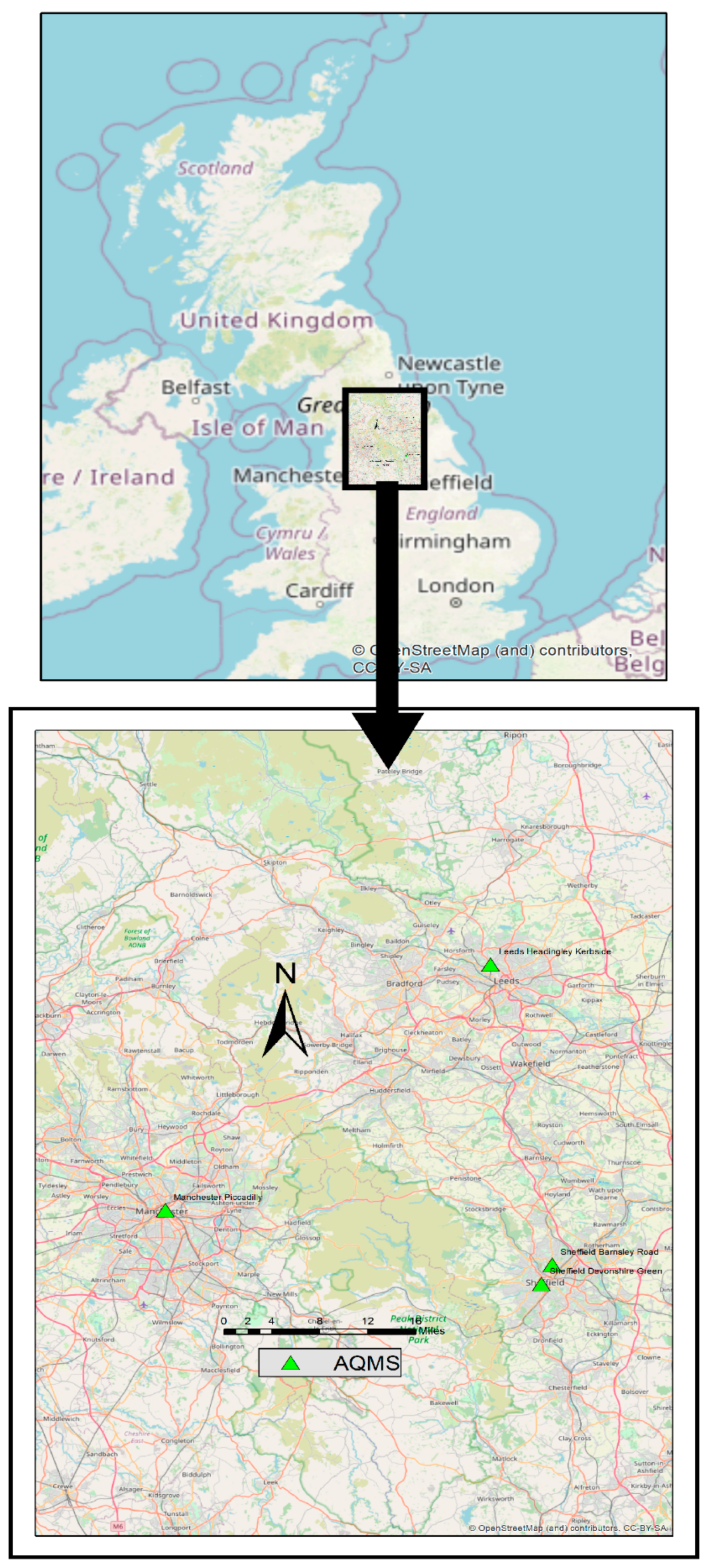
2.1. Study Area and Air Quality Monitoring Stations (AQMS)

In this study, we have selected cities with different sizes and population densities located in the north of England, UK: Leeds, Manchester, and Sheffield. Manchester is the third, Leeds is the fourth, and Sheffield is the seventh-largest city in the UK, with population of 2.84, 2.33, and 1.41 million, respectively (https://www.statista.com/statistics/294645/population-of-selected-cities-in-united-kingdom-uk/ (accessed on 02 March 2021). All these cities have temperate climates and air pollution is considered one of the growing environmental problems. Figure 1 shows the locations of the selected AQMS within the study area, together with a UK map showing the locations of cities under investigation.
The UK has a large network of 170 AQMS covering both urban and rural areas. The network is referred to as the Automatic Urban and Rural Network (AURN) and is operated by the United Kingdom (UK) Department for Environment, Food and Rural Affairs (DEFRA). The AQMS provides measurements of several air pollutants, including NO, NO2, NOx, O3, PM10, and PM2.5. Based on environment types, DEFRA divides the AQMS into three main groups as urban, suburban, and rural sites. These groups are further subdivided into traffic, industrial and background sites to reflect the major source of air pollution in the area. Therefore, there are six categories of AQMS in the AURN: Urban Traffic (UT), Urban Industrial (UI), Urban Background (UB), Suburban Industrial (SI), Suburban Background (SB), and Rural Background (RB). In this study, we have collected data from three UT and one UB AQMS. Table 2 shows the names, geographical coordinates, and environmental types of the AQMS used in this study.

2.2. Air Quality and Meteorological Data

Hourly measured concentrations of several air pollutants are freely available for download at the DEFRA website (https://uk-air.defra.gov.uk/networks/network-info?view=aurn (accessed on 15 January 2021), along with some other important details, e.g., data ratification, quality control, and measurement techniques of these air pollutants. In this study we considered several air pollutants: NO, NO2, NOx, PM2.5, and PM10. Details on the measurement techniques used for these air pollutants are provided on: https://uk-air.defra.gov.uk/networks/monitoring-methods?view=eu-standards (accessed on 15 January 2021). NO, NO2, and NOx are measured by the reference techniques—chemiluminescent analysers, whereas PM10 and PM2.5 are measured using Filter Dynamics Measurement System (FDMS), e.g., Thermo 1405-F FDMS. Manchester Piccadilly AQMS had NO, NO2, NOx, PM2.5, and PM10 measurements for the year 2020 but PM10 data was missing for the year 2019. PM10 data was also missing at Sheffield Barnsley Road AQMS for both 2019 and 2020. Hourly air quality data from the four AQMS were used for 2019 and 2020. Less than 2% of the air quality data were missing in this study. The missing data were ignored as they will not affect the overall results due to the huge amount of data utilised in this study. In addition to air quality parameters, all AURN sites have modelled meteorological data of wind speed (WS), wind direction (WD) and air temperature (Temp), which are estimated by the high-resolution Met Office Model. Meteorological data were used for deweathering the air quality data and producing pollution roses to see the impact of meteorological conditions on air quality during the pre-lockdown, lockdown, and post-lockdown periods. The meteorological data are summarised in Figure 2 in the form of a polar plot, showing how WS, WD, and Temp varied during the pre-lockdown, lockdown, and post-lockdown periods.
To extract the impact of COVID-19 lockdown on the air quality, the air quality datasets were divided into three periods: (i) pre-lockdown (1 February 2020–23 March 2020), (ii) lockdown (24 March 2020–10 May 2020), and (iii) post-lockdown (11 May 2020–30 June 2020).

2.3. Mobility Data

According to Jephcote et al. [29], road traffic counts were down by 70% during the lockdown period as compared to the pre-lockdown period in the UK. Mobility data normalised by 13 January 2020 across the UK for the three cities were obtained from the Apple mobility website, which was grouped into three categories: walking, driving, and public transit [39]. Changes in mobility data as a percentage for the whole UK shown in Figure 3, from 14 January 2020, until 30 June 2020. Figure 3 shows the mobility changes in the form of walking, driving, and public transit. All mobility data showed dramatic decreases from the start of March even before the beginning of COVID-19 lockdown which started on 24 March 2020. Later, mobility data showed a slightly increasing trend since April 2020. Walking has no direct impact on air pollutant emissions; therefore, it was not included in the correlation analysis.

2.4. Building a Generalised Additive Model (GAM)

To investigate the effect of meteorological conditions on air pollutants, researchers, e.g., [29,30,32,33,34], used different statistical and machine learning techniques such as Random Forest, Boosted Regression Trees, and Generalised Additive Models (GAM). Here we adopted the GAM approach used by [30,34], which is an interpretable machine learning approach. Atmospheric air pollutant data often exhibit non-linear behaviour with meteorological parameters and emission sources that hinder the researchers from making straightforward inferences about the fitted model parameters. Several methods have been proposed and thoroughly evaluated from time to time and efforts are made to come up with more effective models for a better understanding of the processes that affect air quality. Consequently, today there are numerous modelling techniques available to researchers such as generalised linear models (GLM) or a more flexible version called GAM. GLM attempts to model a transformed response variable to achieve linearity in regression. However, it is still strictly parametric, and the error distribution follows a valid probability model. GAM is slightly different as it allows the inclusion of non-parametric terms into the model. GAMs are now widely used in the analyses of air pollution, climate change, and its impact on public health and regional ecosystems [40,41,42,43,44]. The fundamental purpose of GAM is to get a smoothed response variable by removing the effect of weather changes and seasonal trends from a given air pollutant concentration, which is called deweathering.
For a given response variable Y regressed over m explanatory variables X 1 , X 2 , . X m an ordinary multiple linear regression model is given in Equation (1),
Y = β 0 + β 1 X 1 + β 2 X 2 + + β m X m + ϵ
where β 0 , β 1 , β 2 , , β m are the model parameters that can be best estimated using the ordinary least square method provided a few assumptions are satisfied such as the response variable is continuous, have symmetric or normal-like distribution, and hence normal errors ( ϵ N 0 , σ 2 ), homogeneity of error variances, and no-multicollinearity among explanatory variables. When these conditions, especially when the response variable depends on an explanatory variable in a non-linear manner or when it is non-continuous (say counts) with a highly skewed distribution (e.g., Poisson), a transformation is usually employed to force the response variable to behave like a linear function of explanatory variables. Using the link function g, GLM links the weighted sum with the mean (average) value of the assumed distribution, as shown in Equation (2):
E Y | X = g β 0 + β 1 X 1 + β 2 X 2 + + β m X m
For which the inverse transformation produces Equation (3):
g 1 E Y | X = β 0 + β 1 X 1 + β 2 X 2 + + β m X m
GAM is a further generalisation of a GLM by adding further non-linear smoothening functions of the explanatory variables. GLM is strictly parametric, i.e., the model shape is predetermined and every explanatory variable in the model has a known association with the response variable. GAM is more flexible in the sense that, based on some link function, it can incorporate non-linear functions of explanatory variables say f X to compensate for the detailed parametric relationships on the explanatory terms to better explain the variation in the response variable. It is equivalent to relaxing the linearity assumption flexibly so that one can learn about the relationship of response and explanatory variables without specifying the actual parametric function of the relationship. A typical GAM with a link function g is given in Equation (4):
g 1 E Y | X = β 0 + f 1 X 1 + f 2 X 2 + + f m X m
For more details on GAM see [45,46].

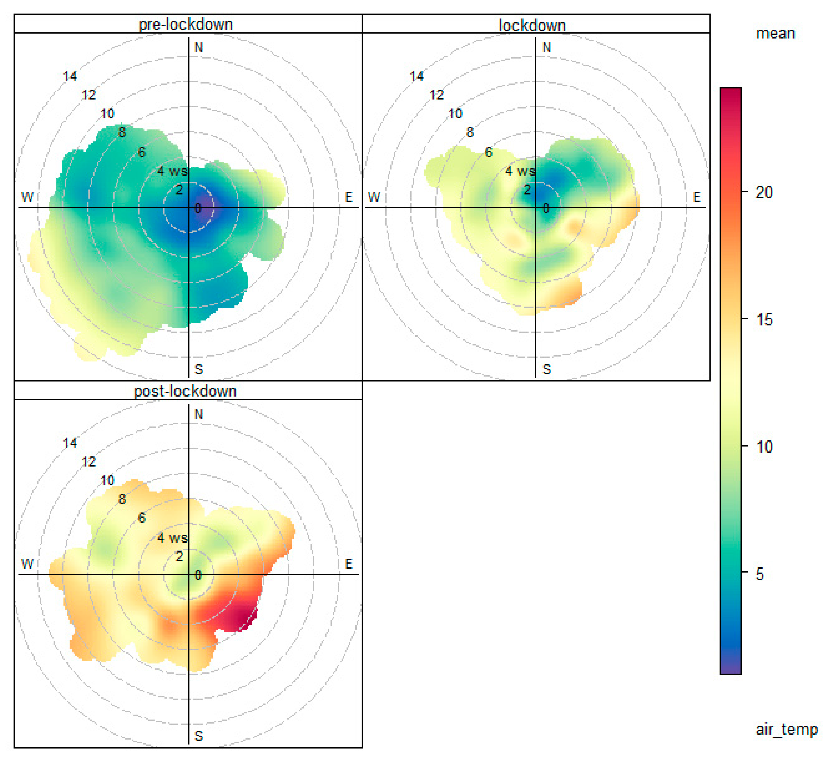
2.5. Statistical Analysis and Deweathering of Air Quality Data

In this study, we used a GAM, an interpretable supervised machine learning technique, to remove the impact of meteorological variations from the air quality data, which is referred to as deweathering or normalising/adjusting the air quality data for meteorological effect, using ‘mgcv’ package [47] in R programming language [48]. Six predictors were used to deweather each air pollutant including three meteorological parameters (WS, WD, and Temp) and three temporal variables (hour of the day, day of the month, and week of the year) to account for temporal variability. Separate deweathering models were developed for 2019 and 2020. Deweathered concentrations have been designated with “dw” annotations. The full dataset was divided into two sub-datasets: training (80%) and testing (20%) datasets. GAM models were fitted (trained) on the 80% training dataset and validated (tested) based on the 20% testing datasets, both randomly selected. The validated models were applied to each year separately to deweather each pollutant for each AQMS. Both measured (raw data) and deweather data are used in this study. Deweathered data present changes in air pollutant concentrations based on variations of the emissions more realistically. Partial deweathering was carried out in this study due to the availability of limited meteorological data (WS, WD, and Temp). Data for other meteorological conditions, such as relative humidity, atmospheric pressure, solar radiations, rainfall and cloud cover were not available. Temporal variation plots and pollution roses plots were developed using openair-package [49] which is a dedicated R programming language package for air quality analysis. Openair back trajectory function was used to calculate back trajectory for identifying the origin of air masses [49].
In this study, we focused on the first lockdown period in the UK, which was from 24 March to 10 May 2020. We used three approaches for assessing the effect of COVID-19 lockdown intervention on air quality. The three main approaches used in this study are as follows:
  • Comparing pre-lockdown, lockdown, and post lockdown periods using data from 2020.
  • Comparing COVID-19 lockdown period in 2020 with the equivalent period in 2019. This approach has the benefit of comparing the same season in different years and therefore produces more realistic results.
  • Comparing mobility trend with the trend of air pollutant concentrations.

3. Results and Discussion

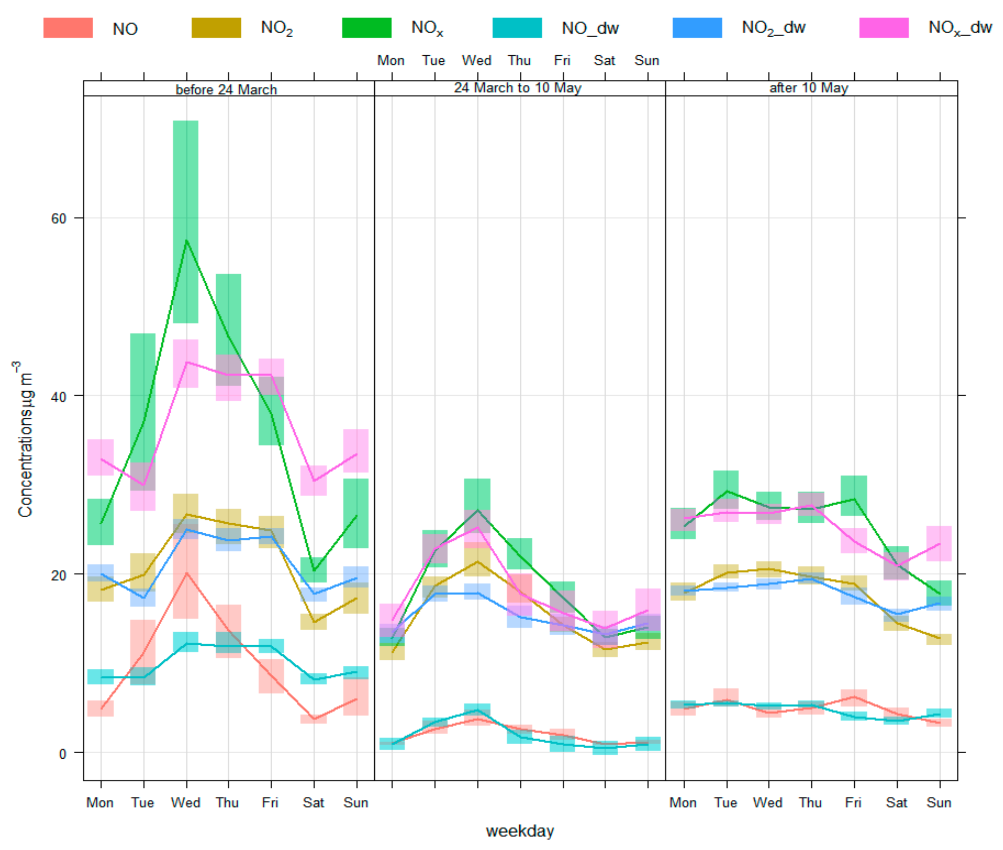
3.1. Changes in Air Pollutant Concentrations during Pre-Lockdown, Lockdown, and Post Lockdown Periods

Table 3 summarises the variations in both measured and deweathered air pollutant concentrations as a percentage (%) for lockdown and post-lockdown periods. The data with ‘dw’ indicates deweathered concentrations for each air pollutant. Hourly air quality data was used in all data analysis. Firstly, mean hourly concentrations of each air pollutant at each period were calculated. Then corresponding mean air pollutant concentration from one period (e.g., pre-lockdown) was deducted from the mean hourly concentrations of this air pollutant from the following period (e.g., lockdown). Finally, the differences in those mean air pollutant concentrations were calculated as percentages (%). The negative sign shows a reduction in air pollutant concentrations while the positive sign indicates an increase in concentration between two successive phases, using the pre-lockdown concentrations as a baseline.
The Sheffield Devonshire Green site is selected because it is the only UB type of station that can serve as a baseline for the area under investigation. The trends of both measured and deweathered data for each air pollutant concentration are illustrated. The weekly cycles of both measured and deweathered NO, NO2, and NOx for pre-lock down, lock-down, and post-lockdown periods at the station are presented in Figure 4.
The levels of NO, NO2, and NOX exhibited substantial reductions during the lockdown period. The mean reductions (%) averaged for all four sites in NO, NO2, and NOx concentrations of deweathered data were 67.20%, 36.58%, and 50.31%, whereas for measured (raw) concentrations were 64.86%, 34.92%, and 47.69%, respectively, during lockdown compared to the pre-lockdown period. Reductions in NO2 concentrations in our study were consistent with the finding of a recent study carried out by Dacre et al [27]. In this study AURN stations in the north and middle England showed lower NO2 concentrations during the period of 17 March–30 April 2020 due to reduced emissions. NO, NO2, and NOx concentrations decreased on average 32% to 50% at roadsides during lockdown [30]. During the post-lock-down period, the mobility restrictions have been lifted in the UK therefore slight increases in NO, NO2, and NOx concentrations were observed. The mean increases in NO, NO2, and NOx concentrations of deweathered data were 5.93%, 16.71%, and 12.81%, correspondingly, during the post-lock down period due to increased emissions from vehicles.
The weekly cycles of NO, NO2, and NOx concentrations exhibited a similar trend during the investigated periods. In general, concentrations of these air pollutants showed an increasing trend from Monday up to Wednesday and then started to decrease from Wednesday until the end of the week. This trend was more noticeable during pre-lockdown and lock-down periods for all air pollutants. The lowest concentrations of NO, NO2, and NOx were observed on weekends (Saturday and Sunday) during pre-lockdown, lockdown, and post-lockdown periods, which is expected as the levels of traffic flows are significantly lower on weekend compared to the weekdays in the UK.
The weekly cycles of both measured and deweathered PM2.5 and PM10 for pre-lock down, lock-down, and post-lockdown periods at Devonshire Green AQMS are given in Figure 5. The weekly variations of both PM10 and PM2.5 showed an almost similar pattern in all three periods (Figure 5). A positive correlation between PM2.5 and PM10 is expected [50]. During the lockdown period, dramatic increases in PM10 and PM2.5 levels were observed in comparison to the pre-lockdown period followed by a slight reduction during the post-lock down period at Devonshire Green AQMS. The mean increases (%) in PM10 and PM2.5 concentrations of deweathered data were 48.02% and 49.34%, respectively, during lockdown compared to the pre-lockdown period which is lower than the mean increases (%) in measured PM10 and PM2.5 concentrations (62.00% and 80.31%), respectively). PM concentrations have increased during the lock-down period at all AQMS under investigation. In general, concentrations of PM levels increased from Monday up to Wednesday and then started to decrease from Wednesday until the end of the week. This trend was more noticeable during pre-lockdown and lock-down periods for all air pollutants. The lowest concentrations of PM were observed on weekends.
In addition to changes in pollutant emissions, a significant change in weather patterns was observed during the pre-lockdown, lockdown, and post-lockdown periods. As an example, we presented meteorological conditions and PM2.5 concentrations from the Manchester site, in the form of pollution rose (Figure 6), which showed how WD, WS, and Temp changed during the three study periods. Figure 6a shows the temperature variations while Figure 6b illustrates the variations in PM2.5 concentrations (µg/m3) with WS and WD at Manchester Piccadilly site. All three meteorological parameters demonstrated considerable variations in their characteristics, which affected the levels of air pollution during the three different periods. During the pre-lockdown wind direction was predominantly south-westerly, bringing clean air from the sea, whereas during the lockdown the wind was easterly and north-easterly bringing polluted air masses from central and eastern Europe. The polluted air masses contained PM from different sources including natural sources. Furthermore, air masses enriched with PM precursors might have increased the formation of secondary PM. Because of these conditions the UK experienced an episode of PM (also shown by [29,31]). The highest easterly wind frequencies during lockdown resulted in peak PM levels at all AQMS. Moreover, frequencies of easterly wind direction were higher during post-lockdown compared to the pre-lockdown period as shown in Figure 6b, which resulted in higher PM concentrations in post lockdown compared to pre-lockdown. Temperature plays an important role in the photochemical reaction and dispersion of locally emitted air pollutants. During high-temperature boundary layer height increases which encourages horizontal and vertical dispersion of pollutants. These meteorological conditions showed that the air pollution episode during the lockdown despite the fact the local emissions had decreased, was caused by the horizontal advection of pollutants from Europe. To further elaborate that during the lockdown period, air masses coming to the UK originated in Europe, we performed back trajectory analysis (Figure 7). Back trajectories in April and February showed totally different origins. The back trajectories in April originated mostly in the eastern Europe bringing polluted air masses to the UK, causing PM episodes during the lockdown periods as the precursors of PM were converted to secondary PM. In February the westerly wind direction brought clean air masses and as a results PM levels were low in the pre-lockdown period. Here we used the back trajectories for London as back trajectories for 2020 were not available for other cities in the UK, at the time of writing this article. However, the same results will be expected for other areas in mid and north England.

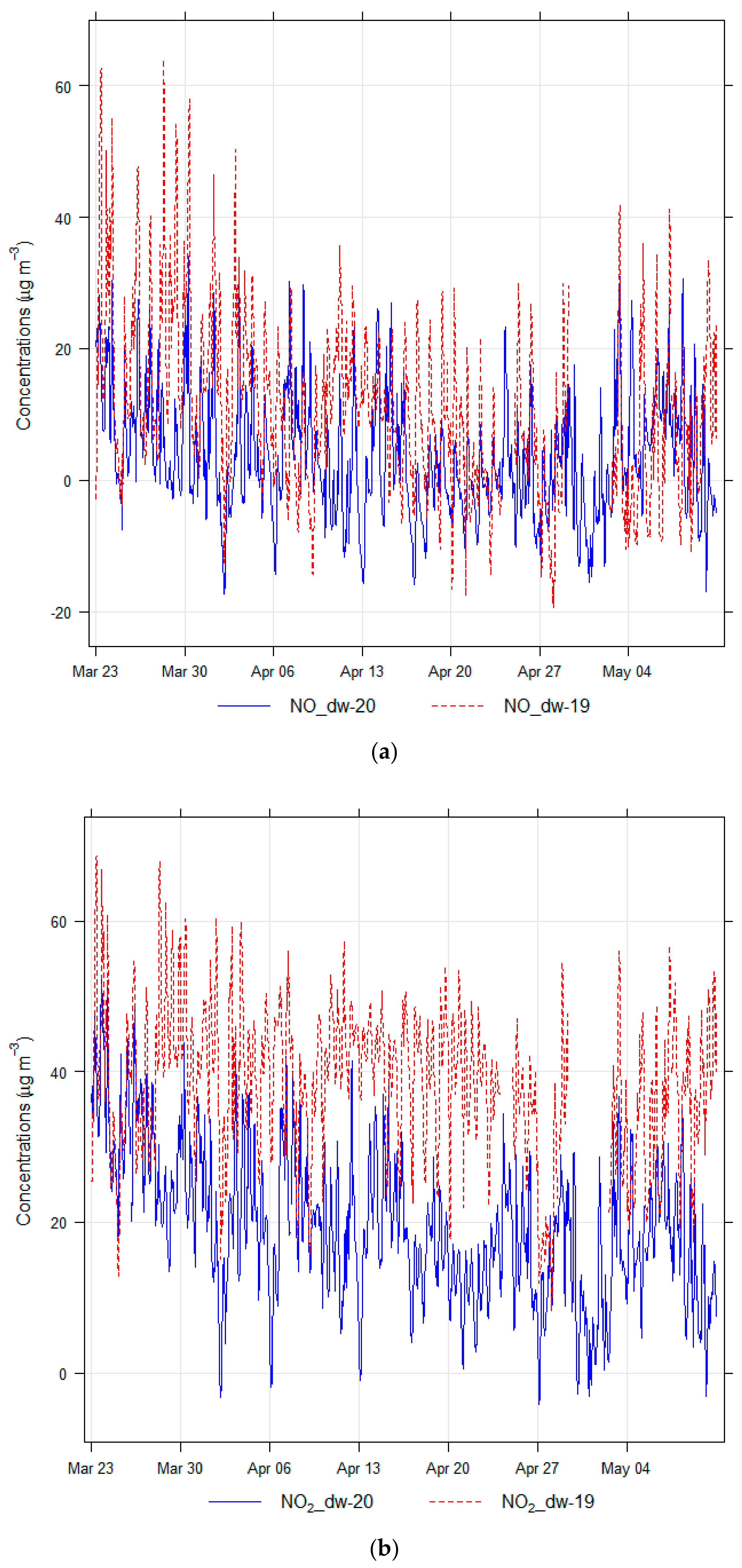
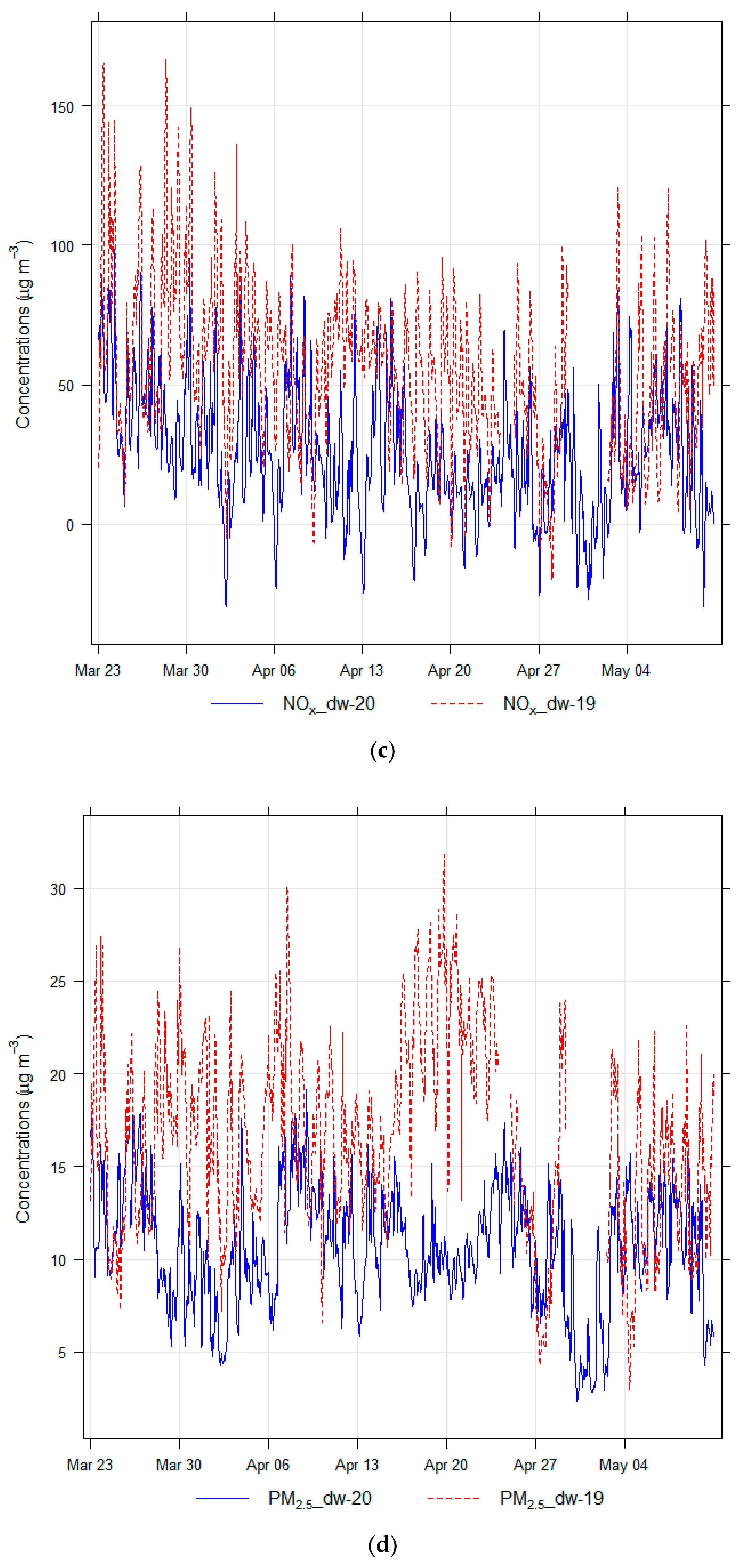
3.2. Changes in Air Quality during Lockdown Period—2020 vs. 2019

Air pollutant concentrations during the lockdown in 2020 were compared with the equivalent period in 2019. Table 4 shows changes in both measured and deweathered pollutant concentrations for the year 2019 vs. 2020. The concentration for each air pollutant in the year 2020 was lower than its measured values in 2019, except for PM10 data at Leeds Headingly AQMS that slightly increased from 22.00 to 22.52 µg/m3. The highest differences in measured concentration were found for NO, NOx, and NO2, respectively. The range of NO reductions was 43.31–69.75%, followed by NOx with 41.52–62.99% and then for NO2 with a reasonably high range between 37.13 and 55.54%. Comparatively, changes in PM concentrations were substantially less: PM10 levels reduced by 19.02% at Sheffield Devonshire Green and increased by 2.36% at Leeds Headingly site. The reduction in PM2.5 concentrations ranged from 29.93% to 40.26%. Changes in the pre-lockdown concentrations between 2019 and 2020 were negligible.
The percentage (%) change between measured and deweathered data was slightly different. The range of changes for NO, NOx, and NO2 were 0.92–4.70%, 0.98–3.89%, and 0.27–0.99%, respectively. On the other hand, the changes for PM10 and PM2.5 concentrations were 0.58–2.46% and 2.01–3.28%, respectively. The deweathering was only based on the WD, WS and temperature; hence, the impact of other influential meteorological factors was not included due to data unavailability, otherwise, the difference between deweathered and measured data would probably have been greater. Figure 8 compares the air quality data during the lockdown period 2020 with the equivalent period in 2019 at Manchester Piccadilly AQMS, which clearly demonstrates reductions in the levels of pollutants.

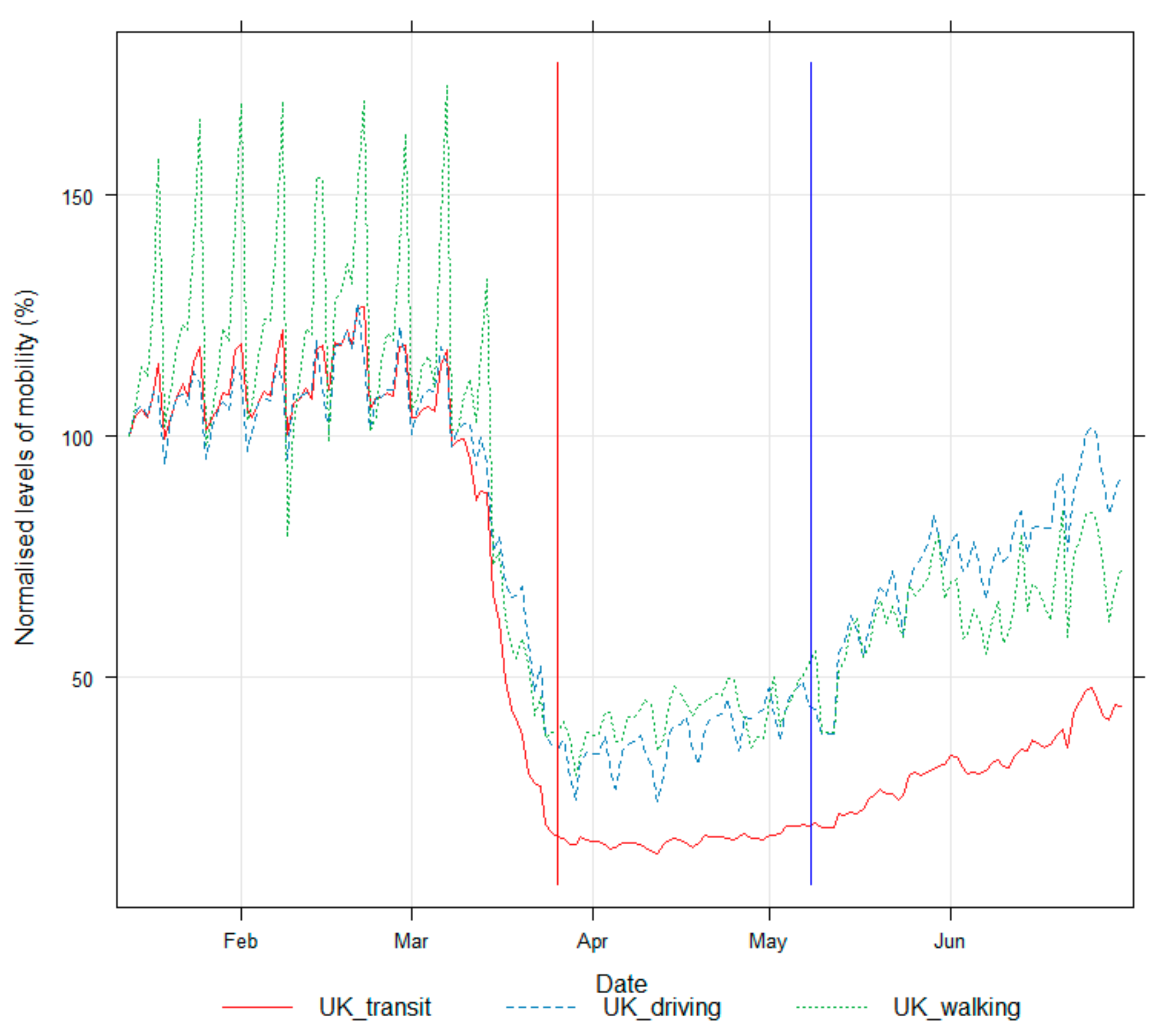
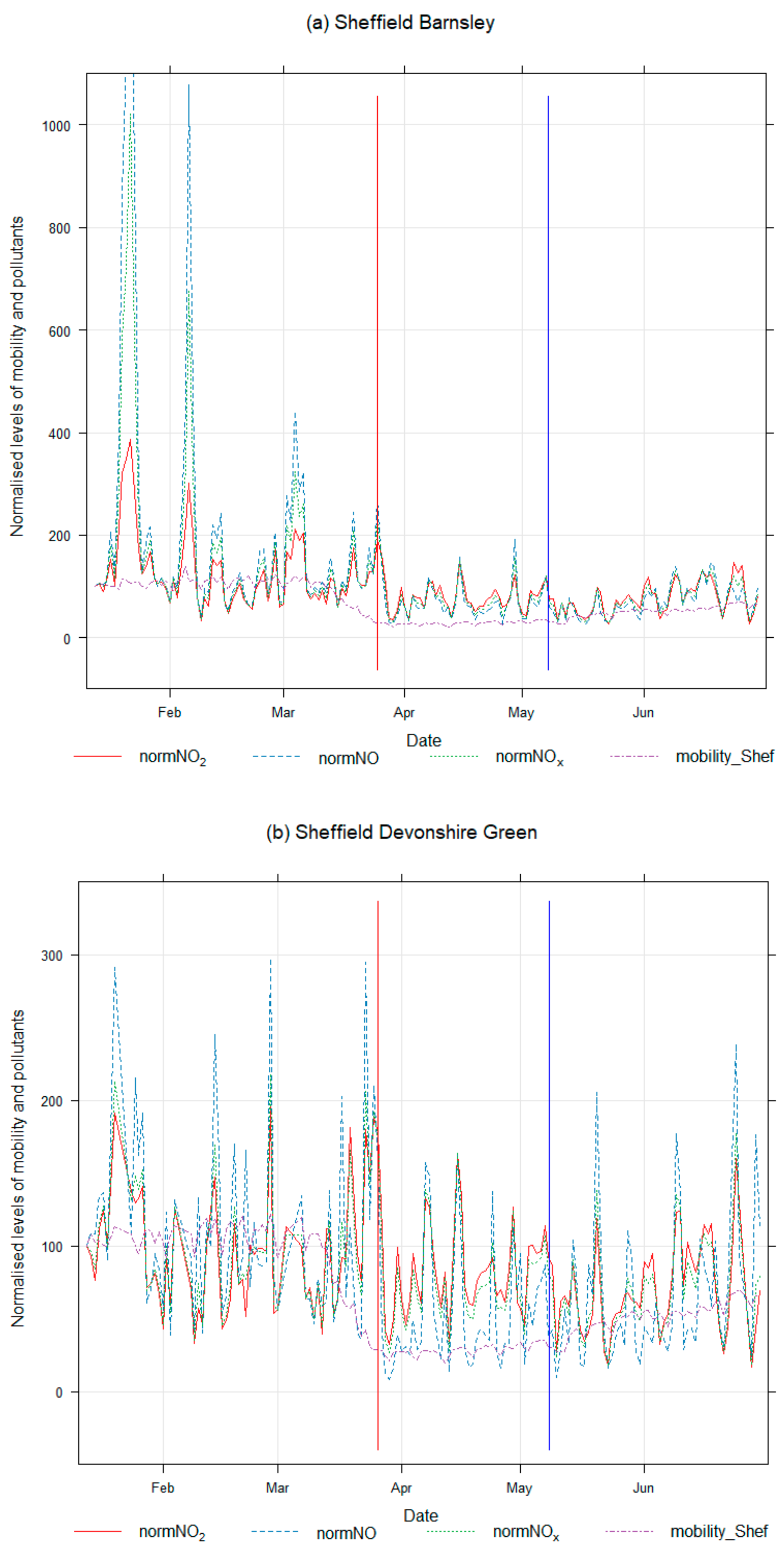
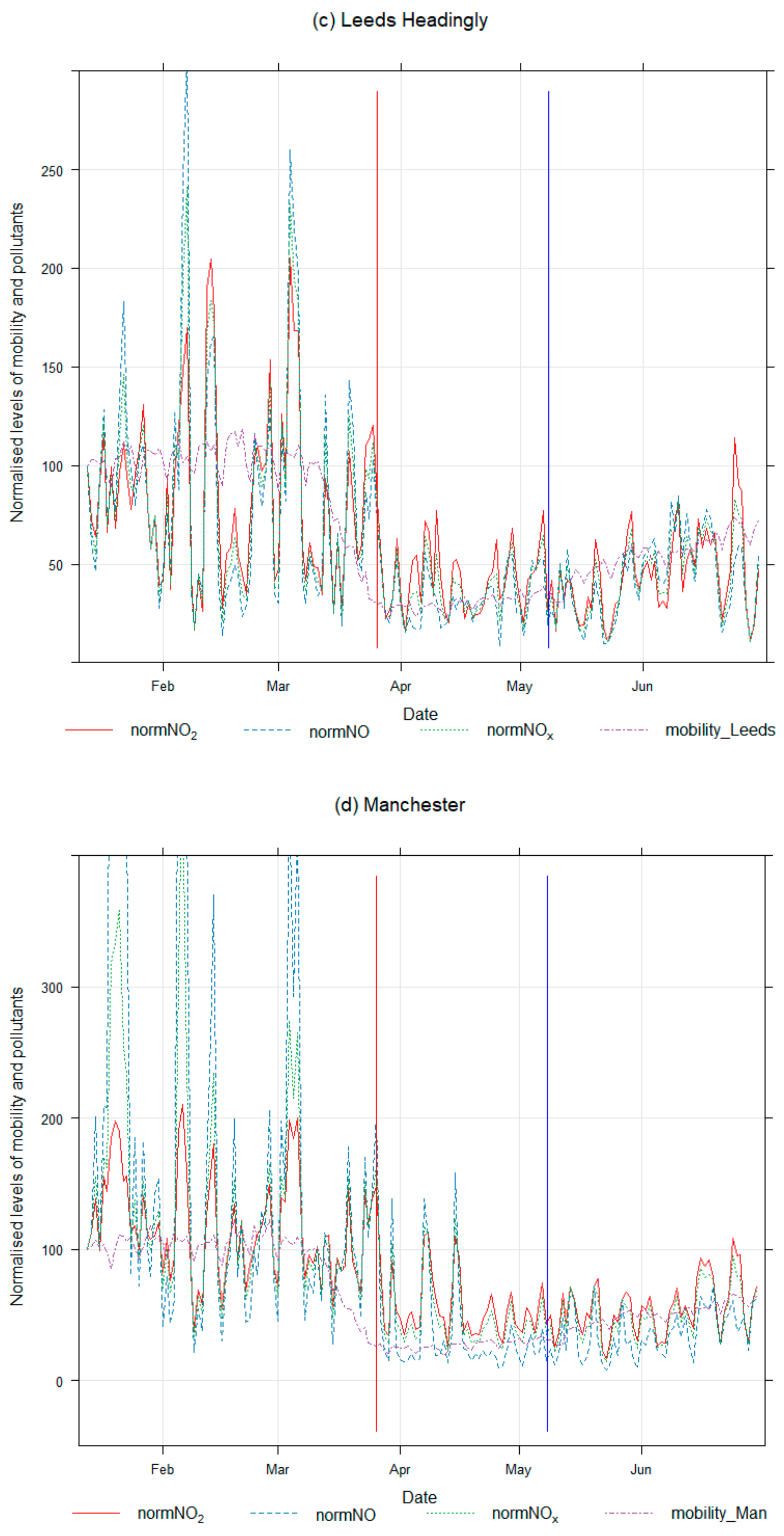
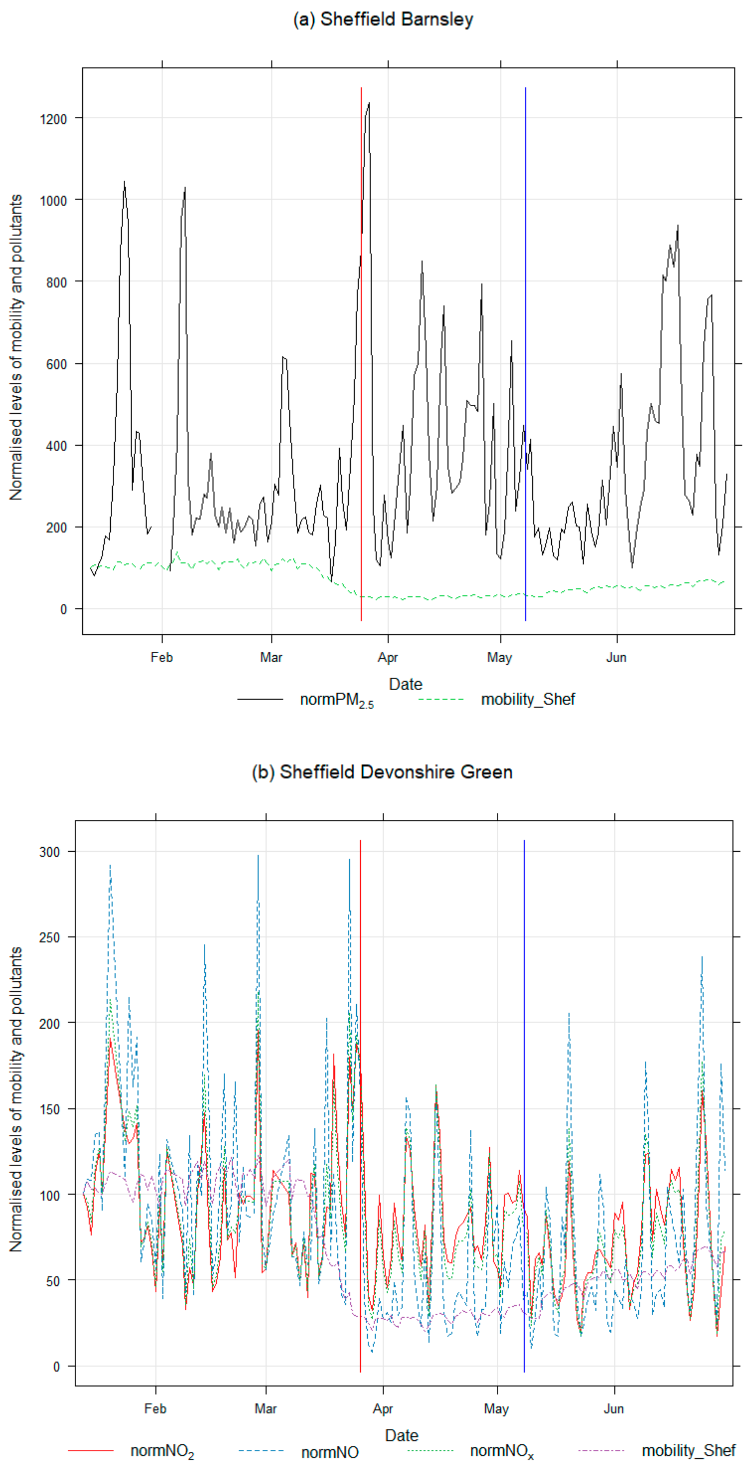
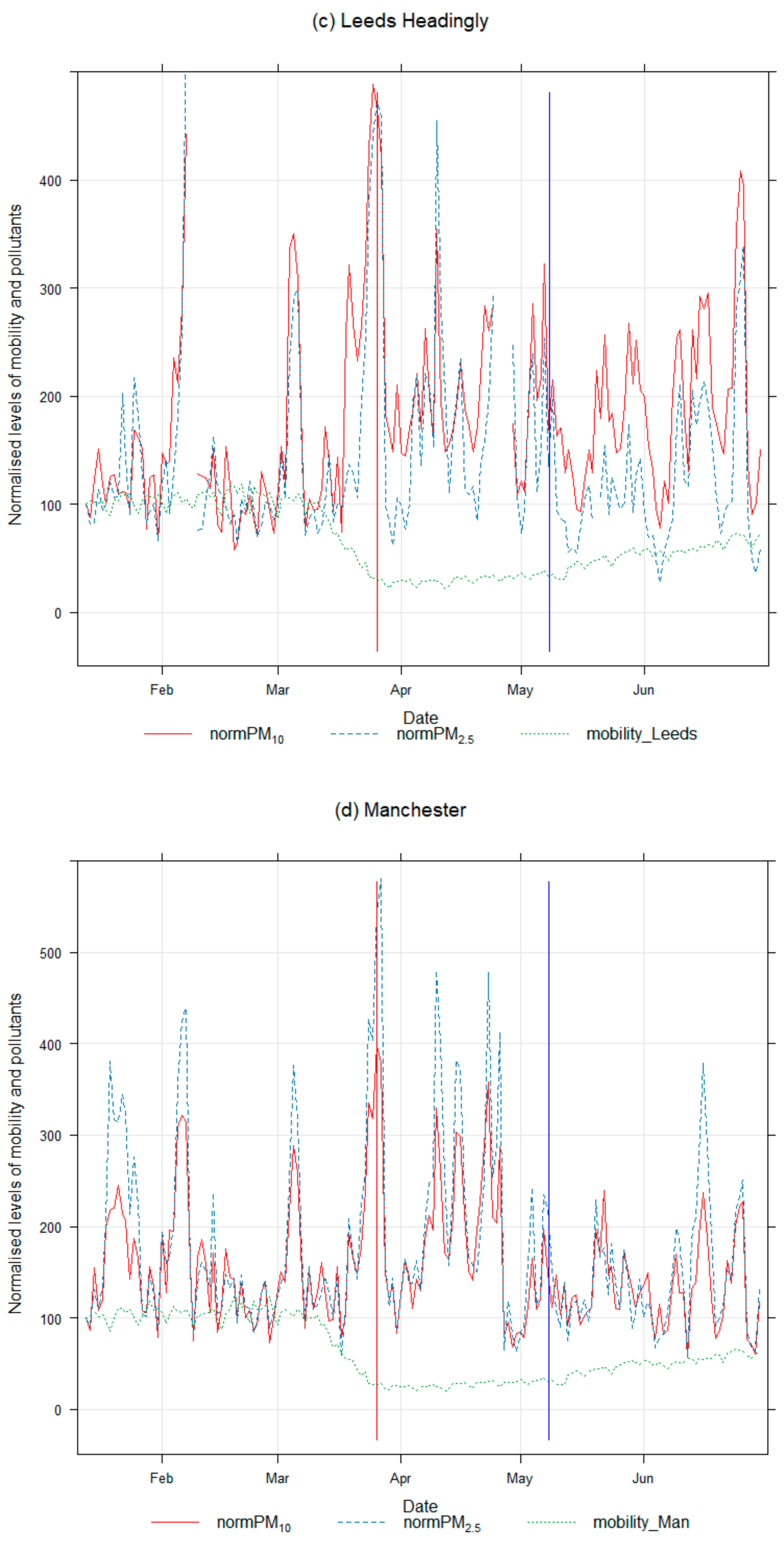
3.3. Relationship between Air Pollutant Concentrations and Mobility

It was expected that a substantial reduction in mobility such as driving and transit (using public transportation) during the lockdown period would reduce vehicular emissions, leading to improvements in air quality. Here we correlated the average of driving and transit trends with different air pollutant concentrations. Generally, NO, NO2, and NOx demonstrated considerable reduction during the lockdown period, however, the reduction was not linear and reduction in the level of mobility was much greater than the reduction in pollutant concentrations. The PM showed an inverse relationship with the levels of mobility. Time series plots of mobility data together with NO, NO2, and NOX at AQMS in Sheffield, Manchester and Leeds covering pre-lockdown, lockdown and post-lockdown periods are shown in Figure 9. Time series plots of PM10 and PM2.5 concentrations with mobility data are shown in Figure 10, showing a weak correlation between PM and mobility at all four sites.
Correlation analysis was performed between mobility data and each air pollutant concentrations to investigate the strength of linear association between them. In this study, absolute values of the correlation coefficient between 0.00 and 0.09 have been considered as negligible correlation, the range between 0.10 and 0.39 as weak correlation and values between 0.40 and 0.69 as moderate correlation. Correlation coefficients between 0.70 and 0.89 were considered as strong correlations while any value over 0.90 was interpreted as a very strong correlation [51]. The values of correlation coefficients are presented in Table 5. In this study, the correlation was either weak or moderate, strong correlation was not observed between the mobility data and any air pollutant.
The highest positive correlation of NO, NO2, and NOx concentrations with mobility were observed at Manchester Piccadilly AQMS, with r-values of 0.48, 0.66, and 0.58, followed by Leeds Headingly with r-values of 0.51, 0.53, and 0.53, respectively. Correlation coefficients for NO, NO2, and NOx concentrations with mobility at Sheffield Devonshire Green and Sheffield Barnsley Rd AQMS were slightly lower than for both Leeds Headingly and Manchester Piccadilly. The population of Manchester, Leeds, and Sheffield are 2.84, 2.33, and 1.41 million, respectively. The correlation analysis showed that larger cities had a stronger correlation between mobility data and pollution levels. A negative correlation was witnessed between mobility data and PM2.5 and PM10 concentrations. The range of correlation coefficient values was between −0.10 and −0.34 for PM10 and −0.10 and −0.26 for PM2.5. According to the observations of this study, PM is not directly associated with mobility data, probably because variations in PM concentrations are more controlled by meteorological conditions and regional PM transportation than by local traffic emission sources. These findings are in agreement with Munir et al. [52], who, using dispersion modeling in Sheffield, found that PM emissions were dominated by points sources, whereas NOx emissions were dominated by road traffic.
According to the current study, the levels of NO, NO2, and NOx have relatively decreased during the lockdown period compared to the control periods (whether pre-lockdown in 2020 or equivalent period in 2019). The NOx species are predominantly emitted by road traffic in urban areas; therefore, their levels in the atmosphere are directly associated with the levels of traffic. However, reductions in road traffic are more than the reductions in atmospheric concentrations (e.g., reduction in road traffic was about 70%, whereas reduction in pollutant levels was much less). The association between air pollutant emissions and their atmospheric concentrations is complicated by several factors including meteorological conditions, boundary layer height and geographical settings.
Changes in the levels of PM10 and PM2.5 during the lockdown period are more controversial. Previous studies have shown conflicting results ranging from reductions to positive gains even in different cities of the same country as shown in Table 1. For example, Donzelli et al. [20] reported +33.0% increase in Pisa and −50.0% reduction in Florence, Italy in the levels of PM2.5. In the UK, similar to the current study, several researchers have reported that the levels of PM10 and PM2.5 have increased [29,30]. In contrast, others have reported that reduction in the levels of PM is much subtler compared to NO2 [28]. Why PM levels have increased or not decreased as much as expected, is a question not yet answered satisfactorily. However, researchers have provided different explanations according to their understanding and based on the local meteorological and emission conditions. Donzelli et al. [20], Marinello et al., [24] and Hormann et al. [22] thought that people used the indoor heating system more frequently as they spent more time indoors during the lockdown, which increased PM emissions. They suggested further research to fully comprehend this matter. Hormann et al. [22] stated that the reduction in traffic levels did not result in a significant reduction in PM10 levels because PM10 pollution in urban areas is not a monocausal phenomenon. They mentioned that increases in indoor residential emissions could be a possible cause for the positive PM10 gain during the lockdown period. In addition, they also mentioned that PM10 values were unusually low in the control group. In addition, Marinello et al., [24] suggested that primary emissions, biomass combustion, PM precursors emissions, meteorological conditions, and the formation of secondary PM could have resulted in the high levels of PM during the lockdown period. Furthermore, industrial sources, harbour emissions, construction works, dust resuspension, regional air mass transport, and Saharan dust episodes could be responsible for the PM episodes [26]. Ropkins and Tate [30] highlighted that public transport, mainly buses which were not stopped in most areas during the UK lockdown, could be a potential source of PM that did not let the PM levels decrease as expected during the lockdown period. Buses are considered as major airborne particle sources due to: (a) tail-pipe emissions from buses, not equipped with diesel particle filters; (b) higher levels of particle resuspension associated with the large frontal area. Shi et al. [29] stated that relative minor reduction in primary PM2.5 emissions from road traffic could be readily overwhelmed by enhanced secondary PM2.5 formation and transportation of PM2.5 from more polluted regions. The conclusion of Shi et al. [29] supports the findings of the current study as we showed using back trajectory that air masses in the UK during the lockdown period originated in central and eastern Europe bringing along polluted air that resulted in the formation of secondary PM formation.
Considering the outcomes of previously published works and the results of our data analysis, the main causes for positive gains or less reduction in PM levels could be summarised as follows:
(a)
Waste burning (as they were not timely collected and people started burning them in their gardens;
(b)
Formation of secondary PM controlled by meteorological conditions and PM emissions precursors;
(c)
Regional transport of PM from other polluted regions;
(d)
Increase in indoor emissions as more people worked from home and used their indoor heating system more frequently, including wood burner stoves;
(e)
Public transport, especially buses, did not stop in many areas during the lockdown period, which did not let the PM levels decrease.
The above analysis showed that sustained improvement in air quality requires actions across various sectors, including cutting local emissions and working with international and European initiatives on long-range transport air pollutants, especially PM2.5.

4. Conclusions

The lockdown period in the UK provided an opportunity to investigate the impact of substantial abrupt reductions in mobility levels on air quality. This study analyses changes in selected air pollutant concentrations due to COVID-19 lockdown measures in Leeds, Sheffield, and Manchester. The non-parametric GAM and other statistical methodologies exhibited significant reductions in NO, NO2, and NOx concentrations during lockdown period, highlighting the influence of reduction in vehicular emissions.
The results demonstrated a stronger positive relationship of mobility with NO, NO2, and NOx concentrations, and a weaker negative relationship with PM10 and PM2.5. In fact, correlation coefficient values for NO, NO2, and NOx were higher for Manchester Piccadilly and Leeds Headingly areas probably showing that the association of pollutant levels with mobility data gets stronger in the cities with heavier traffic. Our results echoed the findings of previous studies which showed that quarantine mobility pattern resulted in immediate and substantial reductions in transportation traffic that reflected upon NO, NO2, and NOx concentrations. On the contrary, PM showed weak association with mobility indicating that PM at the sites included in this study is emitted predominantly by other sources than the road traffic. The weekly cycles of these pollutants during pre-lockdown, lockdown and post-lockdown periods assisted in understanding the consequences of the mobility behaviour on air quality.
Both PM10 and PM2.5 concentrations indicated reasonable increase at all AQMS during lockdown compared with the pre-lockdown period in 2020. However, further statistical analysis of PM10 and PM2.5 concentrations between the lockdown period in 2020 and the equivalent period in 2019 showed that the concentrations of both measured and deweathered data of all air pollutants in 2020 were lower than in 2019. This comparison confirmed that increases in PM levels during the COVID-19 lockdown period was more strongly associated with seasonal variations, and in the absence of lockdown the PM levels would have been even higher. Hence we concluded that COVID-19 lockdown measures have improved the air quality in selected Northern England cities. In this study, both measured and deweathered data was used. The difference in measured and deweathered concentrations was not as much as we expected. This was probably due to the fact that it was a partial deweathering using only WS, WD, and temperature as data for other meteorological parameters like cloud, atmospheric pressure and relative humidity was not available.
As a short-term strategy, UK policymakers should consider a reduction in mobility as a mitigation measure to improve air quality. However, as a long-term strategy, an integrated policy needs to be developed to cut emissions from various sectors and change people’s behaviour towards environmental issues for sustainable air quality improvement. The results of PM recommend investigation of cross-boundary air pollutant transport to analyse dominant source apportionment across Europe as shown with our metrological pollution roses and back trajectory analysis.

Author Contributions

Conceptualization, S.M., G.C., and Y.A.A.; Formal analysis, S.M., G.C., and M.S.J.; Funding acquisition, S.M. and M.M., Methodology, S.M., G.C., M.S.J., and A.A.; Supervision, G.C. and S.M.; Visualisation, S.M., A.A., G.C., and M.S.J.; Writing—original draft, G.C., M.S.J., S.M., Y.A.A., and A.A.; Writing—review and editing, G.C., S.M., M.S.J., A.A., Y.A.A., and M.M. All authors have read and agreed to the published version of the manuscript.

Funding

This research was funded by the Engineering and Physical Sciences Research Council (EPSRC) (grant number—EP/R512175/1) and Siemens plc. The APC was also funded by UKRI/EPSRC.

Data Availability Statement

Publicly available datasets were analysed in this study. This data can be found here: [https://uk-air.defra.gov.uk/networks/network-info?view=aurn (air quality data) and https://www.apple.com/covid19/mobility (mobility data) (accessed on 14 February 2021).

Acknowledgments

We are thankful to the Engineering and Physical Sciences Research Council (EPSRC) (grant number—EP/R512175/1) and Siemens plc for funding this project. The APC was also funded by UKRI/EPSRC.

Conflicts of Interest

The authors declared no potential conflict of interest with respect to the research, authorship and/or publication of this article.

References

  1. WHO. Coronavirus Disease (COVID-19). Available online: https://www.who.int/emergencies/diseases/novel-coronavirus-2019 (accessed on 2 February 2021).
  2. Azevedo, L.; Pereira, M.J.; Ribeiro, M.C.; Soares, A. Geostatistical COVID-19 infection risk maps for Portugal. Int. J. Health Geogr. 2020, 19, 1–8. [Google Scholar] [CrossRef] [PubMed]
  3. Vinceti, M.; Filippini, T.; Rothman, K.J.; Ferrari, F.; Goffi, A.; Maffeis, G.; Orsini, N. Lockdown timing and efficacy in controlling COVID-19 using mobile phone tracking. EClinicalMedicine 2020, 25, 100457. [Google Scholar] [CrossRef] [PubMed]
  4. Kroll, J.H.; Heald, C.L.; Cappa, C.D.; Farmer, D.K.; Fry, J.L.; Murphy, J.G.; Steiner, A.L. The complex chemical effects of COVID-19 shutdowns on air quality. Nat. Chem. 2020, 12, 777–779. [Google Scholar] [CrossRef]
  5. Aina, Y.A.; Van der Merwe, J.H.; Alshuwaikhat, H.M. Spatial and temporal variations of satellite-derived multi-year particulate data of Saudi Arabia: An exploratory analysis. Int. J. Environ. Res. Public Health 2014, 11, 11152–11166. [Google Scholar] [CrossRef] [PubMed] [Green Version]
  6. Gowers, A.M.; Walton, H.; Exley, K.S.; Hurley, J.F. Using epidemiology to estimate the impact and burden of exposure to air pollutants. Philos. Trans. R. Soc. A 2020, 378, 20190321. [Google Scholar] [CrossRef] [PubMed]
  7. Wu, X.; Nethery, R.C.; Sabath, M.B.; Braun, D.; Dominici, F. Air pollution and COVID-19 mortality in the United States: Strengths and limitations of an ecological regression analysis. Sci. Adv. 2020, 6, eabd4049. [Google Scholar] [CrossRef] [PubMed]
  8. Yao, M.; Wu, G.; Zhao, X.; Zhang, J. Estimating health burden and economic loss attributable to short-term exposure to multiple air pollutants in China. Environ. Res. 2020, 183, 109184. [Google Scholar] [CrossRef]
  9. Travaglio, M.; Yu, Y.; Popovic, R.; Selley, L.; Leal, N.S.; Martins, L.M. Links between air pollution and COVID-19 in England. Environ. Pollut. 2021, 268, 115859. [Google Scholar] [CrossRef]
  10. Venter, Z.S.; Aunan, K.; Chowdhury, S.; Lelieveld, J. Air pollution declines during COVID-19 lockdowns mitigate the global health burden. Environ. Res. 2021, 192, 110403. [Google Scholar] [CrossRef]
  11. Kumari, P.; Toshniwal, D. Impact of lockdown on air quality over major cities across the globe during COVID-19 pandemic. Urban Clim. 2020, 34, 100719. [Google Scholar] [CrossRef]
  12. Pacheco, H.; Díaz-López, S.; Jarre, E.; Pacheco, H.; Méndez, W.; Zamora-Ledezma, E. NO2 levels after the COVID-19 lockdown in Ecuador: A trade-off between environment and human health. Urban Clim. 2020, 34, 100674. [Google Scholar] [CrossRef]
  13. Rodríguez-Urrego, D.; Rodríguez-Urrego, L. Air quality during the COVID-19: PM2.5 analysis in the 50 most polluted capital cities in the world. Environ. Pollut. 2020, 266, 115042. [Google Scholar] [CrossRef]
  14. Habibi, H.; Awal, R.; Fares, A.; Ghahremannejad, M. COVID-19 and the improvement of the global air quality: The bright side of a pandemic. Atmosphere 2020, 11, 1279. [Google Scholar] [CrossRef]
  15. Wang, Q.; Li, S. Nonlinear impact of COVID-19 on pollutions–Evidence from Wuhan, New York, Milan, Madrid, Bandra, London, Tokyo and Mexico City. Sustain. Cities Soc. 2021, 65, 102629. [Google Scholar] [CrossRef]
  16. Fu, F.; Purvis-Roberts, K.L.; Williams, B. Impact of the covid-19 pandemic lockdown on air pollution in 20 major cities around the world. Atmosphere 2020, 11, 1189. [Google Scholar] [CrossRef]
  17. Baldasano, J.M. COVID-19 lockdown effects on air quality by NO2 in the cities of Barcelona and Madrid Spain. Sci. Total Environ. 2020, 741, 140353. [Google Scholar] [CrossRef]
  18. Collivignarelli, M.C.; Abba, A.; Bertanza, G.; Pedrazzani, R.; Ricciardi, P.; Miino, M.C. Lockdown for CoViD-2019 in Milan: What are the effects on air quality? Sci. Total Environ. 2020, 732, 139280. [Google Scholar] [CrossRef]
  19. Fenech, S.; Aquilina, N.J.; Vella, R. COVID-19-related changes in NO2 and O3 concentrations and associated health effects in Malta. Front. Sustain. Cities 2021, 3, 631280. [Google Scholar] [CrossRef]
  20. Donzelli, G.; Cioni, L.; Cancellieri, M.; Llopis Morales, A.; Morales Suarez-Varela, M.M. The effect of the Covid-19 lockdown on air quality in three Italian medium-sized cities. Atmosphere 2021, 11, 1118. [Google Scholar] [CrossRef]
  21. Grivas, G.; Athanasopoulou, E.; Kakouri, A.; Bailey, J.; Liakakou, E.; Stavroulas, I.; Kalkavouras, P.; Bougiatioti, A.; Kaskaoutis, D.G.; Ramonet, M.; et al. Integrating in situ measurements and city scale modelling to assess the COVID–19 lockdown effects on emissions and air quality in Athens, Greece. Atmosphere 2020, 11, 1174. [Google Scholar] [CrossRef]
  22. Hörmann, S.; Jammoul, F.; Kuenzer, T.; Stadlober, E. Separating the impact of gradual lockdown measures on air pollutants from seasonal variability. Atmos. Pollut. Res. 2021, 12, 84–92. [Google Scholar] [CrossRef] [PubMed]
  23. Lonati, G.; Riva, F. Regional scale impact of the COVID-19 lockdown on air quality: Gaseous pollutants in the Po Valley, Northern Italy. Atmosphere 2021, 12, 264. [Google Scholar] [CrossRef]
  24. Marinello, S.; Lolli, F.; Gamberini, R. The impact of the COVID-19 emergency on local vehicular traffic and its consequences for the environment: The case of the city of Reggio Emilia (Italy). Sustainability 2020, 13, 118. [Google Scholar] [CrossRef]
  25. Piccoli, A.; Agresti, V.; Balzarini, A.; Bedogni, M.; Bonanno, R.; Collino, E.; Colzi, F.; Lacavalla, M.; Lanzani, G.; Pirovano, G. Modeling the effect of COVID-19 lockdown on mobility and NO2 concentration in the Lombardy region. Atmosphere 2020, 11, 1319. [Google Scholar] [CrossRef]
  26. Tobías, A.; Carnerero, C.; Reche, C.; Massagué, J.; Via, M.; Minguillón, M.C.; Alastuey, A.; Querol, X. Changes in air quality during the lockdown in Barcelona (Spain) one month into the SARS-CoV-2 epidemic. Sci. Total Environ. 2020, 726, 138540. [Google Scholar] [CrossRef]
  27. Dacre, H.F.; Mortimer, A.H.; Neal, L.S. How have surface NO2 concentrations changed as a result of the UK’s COVID-19 travel restrictions? Environ. Res. Lett. 2020, 15, 104089. [Google Scholar] [CrossRef]
  28. Jephcote, C.; Hansell, A.L.; Adams, K.; Gulliver, J. Changes in air quality during COVID-19 ’lockdown’ in the United Kingdom. Environ. Pollut. 2021, 272, 116011. [Google Scholar] [CrossRef]
  29. Shi, Z.; Song, C.; Liu, B.; Lu, G.; Xu, J.; Van Vu, T.; Elliot, R.J.R.; Li, W.; Bloss, W.J.; Harrison, R.M. Abrupt but smaller than expected changes in surface air quality attributable to COVID-19 lockdowns. Sci. Adv. 2021, 7, eabd6696. [Google Scholar] [CrossRef]
  30. Ropkins, K.; Tate, J.E. Early observations on the impact of the COVID-19 lockdown on air quality trends across the UK. Sci. Total Environ. 2021, 754, 142374. [Google Scholar] [CrossRef]
  31. Air Quality Expert Group. Fine Particulate Matter (PM2.5) in the United Kingdom; Crown: New York, NY, USA, 2012. [Google Scholar]
  32. Zhao, Y.; Zhang, K.; Xu, X.; Shen, H.; Zhu, X.; Zhang, Y.; Hu, Y.; Shen, G. Substantial changes in nitrogen dioxide and ozone after excluding meteorological impacts during the COVID-19 outbreak in mainland China. Environ. Sci. Technol. Lett. 2020, 7, 402–408. [Google Scholar] [CrossRef]
  33. Menut, L.; Bessagnet, B.; Siour, G.; Mailler, S.; Pennel, R.; Cholakian, A. Impact of lockdown measures to combat Covid-19 on air quality over western Europe. Sci. Total Environ. 2020, 741, 140426. [Google Scholar] [CrossRef]
  34. Solberg, S.; Walker, S.E.; Schneider, P.; Guerreiro, C. Quantifying the impact of the Covid-19 lockdown measures on nitrogen dioxide levels throughout Europe. Atmosphere 2021, 12, 131. [Google Scholar] [CrossRef]
  35. Lawal, O.; Nwegbu, C. Movement and risk perception: Evidence from spatial analysis of mobile phone-based mobility during the COVID-19 lockdown, Nigeria. GeoJournal 2020, 1–16. [Google Scholar] [CrossRef]
  36. Li, J.; Tartarini, F. Changes in air quality during the COVID-19 lockdown in Singapore and associations with human mobility trends. Aerosol Air Qual. Res. 2020, 20, 1748–1758. [Google Scholar] [CrossRef]
  37. Venter, Z.S.; Aunan, K.; Chowdhury, S.; Lelieveld, J. COVID-19 lockdowns cause global air pollution declines. Proc. Natl. Acad. Sci. USA 2020, 117, 18984–18990. [Google Scholar] [CrossRef]
  38. Munir, S.; Mayfield, M.; Coca, D. Understanding spatial variability of NO2 in urban areas using spatial modelling and data fusion approaches. Atmosphere 2021, 12, 179. [Google Scholar] [CrossRef]
  39. Apple Inc. COVID-19–Mobility Trends Reports. 2020. Available online: https://www.apple.com/covid19/mobility (accessed on 14 February 2021).
  40. Ravindra, K.; Rattan, P.; Mor, S.; Aggarwal, A.N. Generalized additive models: Building evidence of air pollution, climate change and human health. Environ. Int. 2019, 132, 104987. [Google Scholar] [CrossRef]
  41. Bertaccini, P.; Dukic, V.; Ignaccolo, R. Modeling the short-term effect of traffic and meteorology on air pollution in Turin with generalized additive models. Adv. Meteorol. 2012. [Google Scholar] [CrossRef]
  42. Dehghan, A.; Khanjani, N.; Bahrampour, A.; Goudarzi, G.; Yunesian, M. The relation between air pollution and respiratory deaths in Tehran, Iran-using generalized additive models. BMC Pulm. Med. 2018, 18, 1–9. [Google Scholar] [CrossRef]
  43. Frengut, J.; Tomar, A.; Burwell, A.; Francis, R. Analysis of real-time particulate matter (PM 2.5) concentrations in Washington, DC, using generalized additive models (GAMs). In Proceedings of the 2020 Systems and Information Engineering Design Symposium (SIEDS), Charlottesville, VA, USA, 24 April 2020; pp. 1–5. [Google Scholar]
  44. Li, W.; Pei, L.; Li, A.; Luo, K.; Cao, Y.; Li, R.; Xu, Q. Spatial variation in the effects of air pollution on cardiovascular mortality in Beijing, China. Environ. Sci. Pollut. Res. 2019, 26, 2501–2511. [Google Scholar] [CrossRef]
  45. Wood, S.N. Generalized Additive Models: An Introduction with R; Chapman and Hall/CRC: Boca Raton, FL, USA, 2006. [Google Scholar]
  46. Hastie, T.J.; Tibshirani, R.J. Generalised Additive Models; Chapman & Hall: London, UK, 1990. [Google Scholar]
  47. Wood, S. The mgcv Package: Mixed GAM Computation Vehicle with Automatic Smoothness Estimation. Version 1.8–33. 2020. Available online: https://rdrr.io/cran/mgcv/ (accessed on 2 February 2021).
  48. R Core Team. R: A Language and Environment for Statistical Computing. R Foundation for Statistical Computing: Vienna, Austria, 2020. Available online: https://www.R-project.org/ (accessed on 2 February 2021).
  49. Carslaw, D.C. The Openair Manual–Open-Source Tools for Analysing Air Pollution Data. Manual for Version 2.6–6; University of York: New York, NY, USA, 2019. [Google Scholar]
  50. Coskuner, G.; Jassim, M.S.; Munir, S. Characterizing temporal variability of PM2.5/PM10 ratio and its relationship with meteorological parameters in Bahrain. Environ. Forensics 2018, 19, 315–326. [Google Scholar] [CrossRef]
  51. Schober, P.; Christa Boer, M.; Schwarte, L.A. Correlation coefficients: Appropriate use and interpretation. Anesth. Analg. 2018, 126, 1763–1768. [Google Scholar] [CrossRef]
  52. Munir, S.; Mayfield, M.; Coca, D.; Mihaylova, L.S.; Osammor, O. Analysis of air pollution in urban areas with Airviro dispersion model—A case study in the city of Sheffield, United Kingdom. Atmosphere 2020, 11, 285. [Google Scholar] [CrossRef] [Green Version]
Figure 1. Locations of the air quality monitoring stations (AQMS) within the study area in the UK (Source: OpenStreetMap, developed in ArcGIS 10.5.1).
Atmosphere 12 00504 g001
Figure 2. Polar plots of wind speed, wind direction and temperature at Manchester Piccadilly AQMS during pre-lockdown, lockdown, and post-lockdown period, 2020.
Atmosphere 12 00504 g002
Figure 3. Changes in mobility data (%) in the UK during the lockdown period. The vertical red and blue lines show the start and end of the lockdown period, respectively.
Atmosphere 12 00504 g003
Figure 4. Weekly cycles of NO, NO2, and NOx for pre-lock down, lock-down, and post-lockdown periods at Devonshire Green AQMS in Sheffield.
Atmosphere 12 00504 g004
Figure 5. Weekly cycles of PM2.5 and PM10 for pre-lock down, lock-down, and post-lockdown periods at Devonshire Green AQMS in Sheffield.
Atmosphere 12 00504 g005
Figure 6. Pollution roses demonstrating how weather conditions changed during the three periods: changes in temperature linked with wind speed and directions (a); changes in PM2.5 linked with changes in wind speed and directions at the Manchester Piccadilly site (b).
Atmosphere 12 00504 g006aAtmosphere 12 00504 g006b
Figure 7. Hysplit back trajectories centred on the UK for 6 days in April (20 to 25 April) (upper-panel) and 6 days in February (20 to 25 February) 2020 (lower-panel).
Atmosphere 12 00504 g007aAtmosphere 12 00504 g007b
Figure 8. Comparison of deweathered mean hourly air quality data between lockdown period 2020 with the equivalent period in 2019 at Manchester Piccadilly AQMS. (a) NO; (b) NO2; (c) NOX; (d) PM2.5.
Atmosphere 12 00504 g008aAtmosphere 12 00504 g008b
Figure 9. Time series plots between normalised daily mean (%) mobility data and air pollutant concentrations at all AQMS January to June 2020. January 13 is taken as the baseline for normalisation. Vertical red and blue lines show the start and end of the lockdown period, respectively. (a) Sheffield Barnsley; (b) Sheffield Devonshire Green; (c) Leeds Headingley and (d) Manchester.
Atmosphere 12 00504 g009aAtmosphere 12 00504 g009b
Figure 10. Time series plots between daily mean (%) mobility data and PM2.5 and PM10 at all AQMS. January 13 is taken as the baseline for normalisation. Vertical red and blue lines show the start and end of the lockdown period, respectively. (a) Sheffield Barnsley; (b) Sheffield Devonshire Green; (c) Leeds Headingley and (d) Manchester.
Atmosphere 12 00504 g010aAtmosphere 12 00504 g010b
Table 1. Changes in NO2 and particulate matter levels during the COVID-19 lockdown period in 2020 over several European and UK cities.
City, CountryPollutant StudiedReduction (−)/Gain (+)Reference
Barcelona, SpainNO2−50.0%[17]
Madrid, Spain−62.0%
Milan, ItalyPM10−39.5%[18]
Milan, ItalyPM2.5−37.1%
Milan, ItalyNO2−43.1%
Msida, Malta NO2−54.0%[19]
Florence, Italy −36.0%[20]
Pisa, Italy NO2−41.0%
Lucca, Italy −37.0%
Florence, Italy PM10−31.0%,[20]
Pisa, Italy PM2.5 +33.0%
Florence, Italy PM2.5−50.0%
Athens, Greece NO2−32.0%[21]
Athens, Greece PM2.5−18.0%
Graz, AustriaNO2−(35.0% to 41.0%)[22]
Po Valley, Italy NO2 −40.0% [23]
Reggio Emilia, Italy NO2−30.0%[24]
Reggio Emilia, Italy PM10 +46.0%
Milan, Italy NO2−33.0%[25]
Barcelona, Spain NO2−51.0%[26]
Barcelona, Spain PM10−(28.0% to 31.0%)
London, UK NO2−42.0%[27]
Glasgow, UK −30.0%
Belfast, UK −71.0%
Newport, UK −26.0%
Eastbourne, UK +46.0%
Chilbolton Observatory, UK+36.0%
Reading, UK+6.0%
UKNO2−38.0%[28]
UKPM2.5−17.0%
Milan, ItalyNO2−16.0%[29]
Rome, Italy−27.0%
Madrid, Spain−35.0%
London, UK−8.0%
Paris, France−26.0%
Berlin, Germany−11.0%
Rome, ItalyPM2.5−1.0%[29]
Madrid, Spain−24.0%
London, UK+11.0%
Paris, France+27.0%
UKNO2−(32.0% to 50.0%)[30]
Table 2. Names, environment types, and geographical coordinates of the air quality monitoring sites (AQMS).
AQMSLatitude (y)Longitude (x)CodeAQMS Type
Sheffield Devonshire Green53.378622−1.47810SHDGUB
Sheffield Barnsley Road53.404950−1.45582SHBRUT
Manchester Piccadilly53.481520−2.23788MAN3UT
Leeds Headingly53.819972−1.57636LED6UT
Table 3. Variations in air pollutant concentrations (%) during lockdown (LD) and post-lockdown (PLD) periods at all AQMS.
Devonshire GreenSheffiel
Barnsley Rd
Manchester PiccadillyLeeds Headingly
PollutantLDPLDLDPLDLDPLDLDPLD
NOx−35.8111.52−44.714.03−56.525.94−53.757.33
NOx(dw)−44.4912.81−50.304.14−57.427.83−49.020.29
NO2−18.0617.35−27.935.49−46.555.02−47.152.89
NO2(dw)−22.7016.71−31.634.19−46.397.44−45.593.50
NO−68.2615.99−56.682.30−74.169.33−60.3520.97
NO(dw)−77.595.93−62.744.03−76.129.86−52.353.15
PM1062.00−6.02N/AN/A21.96−29.0930.86−14.87
PM10(dw)48.02−12.58N/AN/A14.45−29.0826.04−15.77
PM2.580.31−27.2441.43−17.6736.24−35.7943.87−35.93
PM2.5(dw)49.34−29.4645.94−17.5623.05−35.4529.59−36.25
Note: Lockdown = Lockdown mean concentration—Pre-lockdown mean concentration as percentage (%). Post-lockdown = Post-lockdown mean concentration—Lockdown mean concentration as percentage (%).
Table 4. Change (%) in air pollutant concentrations during the lockdown in 2020 as compared with the same period in 2019 at all AQMS, where dw = deweathered, diff = difference.
Sheffield DevonshireBarnsley RdManchester PiccadillyLeeds Headingly
Air Pollutant(ug/m3)
2019
(ug/m3)
2020
(%)
Diff.
(ug/m3)
2019
(ug/m3)
2020
(%)
Diff.
(ug/m3)
2019
(ug/m3)
2020
(%)
Diff.
(ug/m3)
2019
(ug/m3)
2020
(%)
Diff.
NO32.3818.3643.3123.7112.7846.079.913.3366.4021.826.6069.75
NO(dw)31.7017.6844.2323.8012.0949.2210.753.2070.2221.657.5665.05
NO225.8515.2940.8337.5923.6437.1338.3018.8050.9030.3713.5055.54
NO2(dw)25.5115.0241.1037.1423.0038.0638.1619.0150.1930.1013.6854.55
NOx4.262.0053.1273.9443.2441.5253.5023.9155.3063.8223.6262.99
NOx(dw)4.061.7557.0173.6941.5443.6354.6423.8856.2863.2525.2560.07
PM1024.5419.8719.02N/AN/AN/AN/AN/AN/A22.0022.522.36
PM10(dw)24.2219.4719.60N/AN/AN/AN/AN/AN/A22.1022.080.10
PM2.519.6211.7240.2620.9512.6739.5317.2511.1535.3817.5312.2929.93
PM2.5(dw)19.4310.9743.5420.4311.7342.5816.6210.5736.4217.1811.6931.94
Table 5. Correlation analysis between mobility data and air pollutant concentrations at different monitoring stations during the lockdown period.
Location of AQMSAir PollutantCorrelation CoefficientType of Correlation
Sheffield Devonshire GreenNO
NO2
NOx
PM10
PM2.5
0.30
0.35
0.33
−0.28
−0.26
Weak positive
Weak positive
Weak positive
Weak negative
Weak negative
Sheffield Barnsley RdNO
NO2
NOx
PM10
PM2.5
0.39
0.45
0.41
N/A
−0.10
Weak positive
Moderate positive
Moderate positive
N/A
Weak negative
Manchester PiccadillyNO
NO2
NOx
PM10
PM2.5
0.48
0.66
0.58
−0.10
−0.10
Moderate positive
Moderate positive
Moderate positive
Weak negative
Weak negative
Leeds HeadinglyNO
NO2
NOx
PM10
PM2.5
0.51
0.53
0.53
−0.34
−0.19
Moderate positive
Moderate positive
Moderate positive
Weak negative
Weak negative
Publisher’s Note: MDPI stays neutral with regard to jurisdictional claims in published maps and institutional affiliations.

