Improvement of Global Ionospheric TEC Derivation with Multi-Source Data in Modip Latitude

Abstract

Global ionospheric total electron content (TEC) is generally derived with ground-based Global Navigation Satellite System (GNSS) observations based on mathematical models in a solar-geomagnetic reference frame. However, ground-based observations are not well-distributed. There is a lack of observations over sparsely populated areas and vast oceans, where the accuracy of TEC derivation is reduced. Additionally, the modified dip (modip) latitude is more suitable than geomagnetic latitude for the ionosphere. This paper investigates the improvement of global TEC with multi-source data and modip latitude, and a simulation with International Reference Ionosphere (IRI) model is developed. Compared with using ground-based observations in geomagnetic latitude, the mean improvement was about $10.88\%$ after the addition of space-based observations and the adoption of modip latitude. Nevertheless, the data from JASON-2 satellite altimetry and COSMIC occultation are sparsely-sampled, which makes the IRI TEC a reasonable estimation for the areas without observation. By using multi-source data from ground-based, satellite-based and IRI-produced observations, global TEC was derived in both geomagnetic and modip latitudes for 12 days of four seasons in 2014 under geomagnetic quiet conditions. The average root-mean-square error (RMSE) of the fitting was reduced by $7.02\%$ in modip latitude. The improvement was largest in March and smallest in June.

1. Introduction

The ionosphere is the ionized part of Earth’s upper atmosphere, in the range of 60~1000 km above the ground. Excited by solar radiation, it contains free electrons deteriorating the propagation of radio waves in the L-band. Radio signals of satellite systems, such as Global Navigation Satellite Systems (GNSSs), traveling through the ionosphere are delayed in time and advanced in phase, which are proportional to the integration of electron density along the signal propagation path and referred to as total electron content (TEC). This provides a means to obtain TEC from the differences in time delays or phase advances of dual-frequency satellite observations. With the rapid development of GNSS applications, global TEC has been effectively measured at low-cost with ground-based GNSS receivers.

In TEC derivation from GNSSs, the task of assessing differential code biases (DCBs), which originate in the hardware of the satellite and the receiver, and obtaining absolute TEC has been assumption-dependent and time-consuming. Numerous papers have studied the TEC derivation methods and various algorithms have been intensively developed and improved for the last several decades [1,2,3,4,5,6,7,8,9,10,11]. TEC and DCB estimations were first developed in the ionospheric derivation by a single station [1], and then applied to multiple stations in network [2]. Daily global TEC and DCBs are routinely generated with more receivers being set up [3]. Currently, the International GNSS Service (IGS) provides global ionospheric maps (GIMs) and DCB estimations based on the results from seven members called Ionospheric Associate Analysis Centers (IAACs), each of which uses an individually developed algorithm based on ground-based GNSS observations to provide ionosphere products, and IGS combines these products with corresponding weights [4]. Global TEC data from the Center for Orbit Determination in Europe (CODE), European Space Agency (ESA) and Natural Resources Canada (NRCan/EMR) are obtained from series of spherical harmonic (SH) functions up to 15 degrees and orders but with several differences in details [5,6,7]. The Jet Propulsion Laboratory (JPL) uses a linear composition of bi-cubic splines with 1280 spherical triangles and the Polytechnic University of Catalonia (UPC) uses a rectangular grid with two layers model and an interpolation scheme [8,9]. Wuhan University (WHU) obtains the global TEC by using a SH function and inequality-constrained least-squares method, and the approach used by Chinese Academy of Sciences (CAS) is integrating the spherical harmonic and the generalized trigonometric series functions on global and local scales, respectively [10,11]. However, comparative research has shown that the relative errors between GIMs from different centers can reach 20~30% in equatorial and oceanic areas of the Southern Hemisphere where the ground observation is not sufficiently set or there is no observation [12].

Recently, satellite-based observations have been used together with ground-based GNSS observations to improve GIM results. Satellite altimetry missions such as JASON-2/3 provide precise ionospheric information over the oceanic areas, and low-Earth orbiting (LEO) satellites such as Constellation Observing System for Meteorology, Ionosphere, and Climate (COSMIC) occultation provide well-distributed information about the ionosphere on a global scale, which can be powerful supplements to the ground-based observations. Alizadeh et al. [13] obtained GIMs in geomagnetic latitude through combining observations from GNSS, satellite altimetry and occultation measurements, and the results show that the root-mean-square error (RMSE) of the combined GIMs is decreased when compared with the results of fitting with ground-based GNSS data. Yao et al. [14] derived global TEC with ground-based GNSS, satellite altimetry and COSMIC observations in a solar-geomagnetic reference frame using an SH function. The performance of using both ground- and satellite-based data has been improved and was validated by satellite altimetry observations over long periods. Since satellite observations have been sparsely sampled, their supplementary effect on ground-based observation is limited. For obtaining TEC on a global scale, estimation from empirical ionosphere models plays an important role for those areas with limited observations. An et al. [15] used observations of multi-GNSS and satellite altimetry, and a priori values from an International Reference Ionosphere (IRI) model to map the ionosphere in a solar-geomagnetic reference frame, and the validation results suggest the GIMs from this model are further improved through employing multi-source data, especially for the ionosphere over the oceans. Later, the same group only used ground-based observations and the IRI model to obtain the GIMs, and concluded their method has a higher precision than IGS GIMs, even for ionosphere disturbances during geomagnetic storms [16].

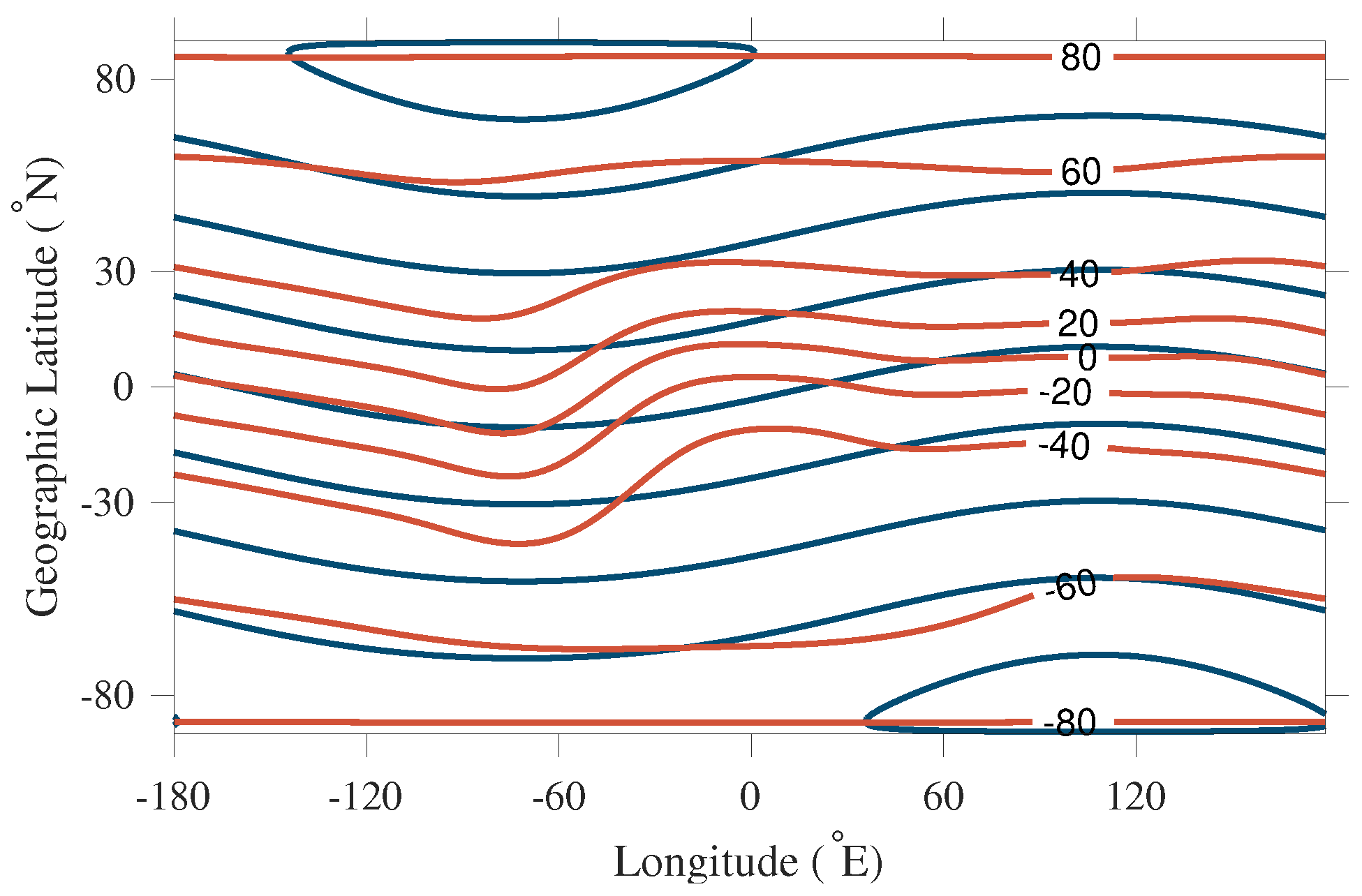
The coordinate system is another important factor since an unsuitable one has a risk of over fitting and spurious peaks. The dip latitude calculated from magnetic elements is unsuitable for global mapping of the ionosphere due to the anomaly of meridional variation near South Africa, and the usual solution of geomagnetic latitude defined by the dipole approximation does not coincide with the true magnetic equator, and is distorted from the real magnetic field of the Earth [17]. In 1963, Rawer [18] introduced the modified dip (modip) latitude, and investigated the benefits of describing the variability of TEC at low and middle latitudes in 1984 [19]. Azpilicueta et al. [20] used ground-based GNSS data in a modip latitude to derive the global ionospheric TEC, and results show that the accuracy of global vertical TEC (VTEC) representation was improved by more than $10\%$ compared with fitting in geomagnetic latitude, particularly in the region of the equatorial anomaly. This suggests that the modip latitude is more suitable for TEC derivation through fitting with observation in the global scale. However, this performance was only studied over three months (March, April and May) of 1999 and validated in areas with existing Topex observations, so the improvement is not clear from a global perspective.

We conclude therefore that the impact of multi-source data and the coordinate system on global TEC derivation is still an open question. Simulation and data analysis can enhance our understanding. In this paper, Section 2 introduces the multi-source data and analysis method in the global ionospheric TEC derivation. In Section 3, due to the non-homogeneous distribution of observational data on a global scale, we study the impacts of data distribution and coordinate system in global TEC derivation by using the reference data generated from the IRI-2016 model. In Section 4, global TEC are derived in a solar-modip coordinate system using an SH function with multi-source data, including observations from GNSS, satellite altimetry (JASON) and occultation (COSMIC), and virtual observations from the IRI-2016 model. Data for 12 days in quiet geomagnetic conditions for four seasons in 2014 were collected and processed, and the final results were examined.

2. Data and Analysis Method

2.1. Ionospheric Observation Data

2.1.1. Observation of GNSS from IGS

TEC can be derived from dual-frequency measurements due to the dispersive characteristics of the ionosphere. IGS had deployed around 400 GNSS dual-frequency receivers worldwide in 2014, which can monitor the global ionosphere all day. The pseudoranges and carrier phases measured at $f_1$ and $f_2$ are used to calculate the slant TEC (STEC) from a satellite to a receiver as

$$STE{C}_{sp}=\frac{2{\left(f_1{f}_2\right)}^2}{k(f_1^2-f_2^2)}(P_2-P_1),$$

(1)

$$STE{C}_{sl}=\frac{2{\left(f_1{f}_2\right)}^2}{k(f_1^2-f_2^2)}(L_1{\lambda }_1-L_2{\lambda }_2),$$

(2)

where $k=80.62$ ${\mathrm{m}}^3·{\mathrm{s}}^{-2}$ is ionospheric refraction, $P_1$, $P_2$ and $L_1$, $L_2$ are distances (pseudorange) and phase measurements, ${\lambda }_1$ and ${\lambda }_2$ are the wavelength of the signal [21].

2.1.2. Observation from JASON-2 Satellite Altimetry

Observations from JASON-2 have a temporal resolution of 1s but only cover ocean areas. Since the ionospheric effects on electromagnetic wave paths are proportional to the density of free electrons and inversely proportional to the square of the frequency of the electromagnetic wave, the altimeter (Ku and C dual-band emission) equipped on JASON-2 can provide ionospheric range correction from the sea level up to the satellite orbit altitude. The measurement error caused by the instrument hardware, satellite attitude, waves or other factors is usually no more than 2~3 TECU (1 TECU = ${10}^{16}e/{\mathrm{m}}^2$), and the credibility of JASON-satellite-derived VTEC at low latitudes and equatorial regions is high [22].

2.1.3. Observation from COSMIC Occultation

The occultation system of COSMIC has advantages of high accuracy and vertical resolution in global coverage. For COSMIC data, VTEC at the position of maximum electron density of every occultation event can be obtained in the ‘ionPrf’ products provided by the COSMIC Data Analysis and Archive Center (CDAAC). The DCBs in COSMIC systems have already been eliminated, therefore further processing is unnecessary.

2.2. Analysis Method

2.2.1. Single-Layer Assumption

In ionospheric research, VTEC or the absolute TEC, which refers to the total electron content along the path that passes through the ionosphere perpendicularly, are generally used. In this paper, the single-layer (SL) assumption is adopted to convert to VTEC from STEC, where all free electrons are assumed to be contained in a shell of infinitesimal thickness at the height above the ground [23]. The altitude of this idealized layer is usually set to 350, 400, or 450 km above a spherical Earth, which approximately corresponds to the altitude of maximum electron density [7]. In this assumption, $\alpha$ is the elevation of satellite S from receiver R, $\chi$ is the zenith angle and P is the ionospheric piercing point (IPP), which is the intersection of the ionosphere and sight line. The zenith angle can be calculated as

$$\chi =arcsin\frac{R_{e}cos\alpha }{R_e+h},$$

(3)

where h is the height of the SL assumption above the ground, and we set $h=450$ km in this paper.

According to Equations (1) and (2) in the TEC obtainment from GNSS, $STE{C}_{sl}$ is a relative value due to the $2\pi$ ambiguity in the phase measurement but $STE{C}_{sp}$ contains more noise than $STE{C}_{sl}$ [24]. High precise STEC can be obtained through carrier-phase smoothing over the pseudorange from GNSS observations after a baseline for the differential phase related $STE{C}_{sl}$ is introduced as [9,25].

$$STE{C}_G=STE{C}_{sl}+\frac{{\sum }_{i=1}^n(TE{C}_{s{p}_i}-TE{C}_{s{l}_i}){sin}^2{\alpha }_i}{{\sum }_{i=1}^n{sin}^2{\alpha }_i},$$

(4)

where n is the number of measurements without a cycle slip. To reduce the multi-path effect at a low elevation angle, the square sine of the satellite’s elevation is included as a weighting factor and the cutoff angle is set as ${25}^{\circ }$ in this paper. Then the $VTE{C}_G$ at the piercing point in the SL assumption can be calculated, where $B_s$ and $B_r$ represent the DCBs from satellites and receivers:

$$VTE{C}_G=(STE{C}_G-B_s-B_r)cos\chi .$$

(5)

Additionally, according to Brunini et al. [26], $VTE{C}_A$, which represents the VTEC obtained from JASON-2 satellite altimetry, can be calculated as

$$VTE{C}_A=-\frac{dR·f_{ku}^2}{40.3},$$

(6)

where $dR$ is the Ku-band ionospheric range correction, and $f_{ku}$ is the Ku-band frequency of 13.575 GHz. Besides, $VTE{C}_A$ needs a 21 s smoothing window to reduce the inherent noise effects of the altimeter [27].

$VTE{C}_C$, the VTEC obtained from the ionPrf product of COSMIC occultation, can be expressed as

$$VTE{C}_C=VTE{C}_0+VTE{C}_1,$$

(7)

where $VTE{C}_0$ is the VTEC under the COSMIC satellite orbit, and $VTE{C}_1$ is the VTEC above the COSMIC satellite orbit calculated by extrapolation [28].

2.2.2. Spherical Harmonic Function

In our method, observations are combined and fitted by an SH function with a degree and order of $n_{max}$ as an interpolation technique to derive the global ionosphere, which can be expressed as:

$$\begin{array}{c}\hfill VTEC(\varphi ,\lambda )={\displaystyle \sum _{n=0,m=0}^{n_{max}}}{\tilde{P}}_{nm}(sin\varphi )({\tilde{A}}_{nm}cos\left(m\lambda \right)+{\tilde{B}}_{nm}sin\left(m\lambda \right)),\end{array}$$

(8)

where $n_{max}$ is the maximum degree of the SH expansion, ${\tilde{P}}_{nm}$ is the normalized associated Legendre function of degree n and order m, ${\tilde{A}}_{nm}$ and ${\tilde{B}}_{nm}$ are the unknown coefficients to be determined, $\varphi$ and $\lambda$ are the latitude and longitude of IPPs.

2.2.3. Modip Coordinate System

The performance of GIM construction strongly depends on using a coordinate system where ionospheric variability is able to be as smooth as possible in space and time [20]. The geomagnetic (GM) latitude of the usual solution is defined similar to geographic latitude but rotated to coincide the geographic pole to the dipole axis. However, the actual magnetic field is not a simple dipole and is distorted. The ‘modified dip’ or the ‘modip’ latitude ($\mu$) is a more suitable magnetic coordinate system for describing the variability of the ionosphere at mid- and low-latitude areas, which is calculated directly from the three components of Earth’s magnetic field fitted by the International Geomagnetic Reference Field (IGRF) model, and is defined as [19]

$$tan\mu =\frac{I}{\sqrt{cos\phi }},$$

(9)

where I is the true magnetic dip and $\phi$ is the geographic latitude. The modip equator is the locus of points where the magnetic dip (or inclination) is 0.

The comparison of geomagnetic latitude (blue) and modip latitude (red) in September 2014 is shown in Figure 1, where the difference between geomagnetic latitude and modip latitude in the equatorial region is obvious. In principle, the modip coordinate system is more suitable for global ionosphere mapping, since it is parallel to the magnetic equator at low latitudes and the spacing is dense in the equatorial area.

2.2.4. Error Analysis

Several important evaluation metrics, such as mean absolute error (MAE), mean error (ME), and root-mean-square error (RMSE), can be used for quantifying the performance. Here we choose RMSE, which is used to represent the accuracy of the model value relative to the measured value, to specify the precision [29]. The expression of RMSE is defined as

$$\mathrm{RMSE}=\sqrt{\frac{1}{N}{\displaystyle \sum _{i=1}^N}{(y_f-y_r)}^2},$$

(10)

where N is the number of derived values, $y_f$ and $y_r$ are the fitting and reference values, respectively, and $(y_f-y_r)$ represents the fitting residual.

3. Simulation

Simulation was performed to understand the impacts of using multi-source data and a modip coordinate system. We used IRI-2016 to obtain the ‘true’ global TEC, evenly-distributed (ED) with a resolution of ${2.5}^{\circ }\times 5^{\circ }\times 0.1$ h in latitude, longitude and time, respectively. The IRI model source code (in FORTRAN) can be accessed on the homepage at http://irimodel.org (accessed on 28 March 2021). The flag of the ‘URSI foF2 model’ was triggered on and the scenarios from the database were used. The global TEC were fitted with SH functions in both geomagnetic and modip latitudes, and the results were analyzed. We compared the RMSE of different degrees and orders in the SH functions; the comparisons are not shown here but the main conclusions remain unchanged. Considering the time consumption and computer capacity, as well as references Schaer [7], Yao et al. [14] and An et al. [15], an SH function with a degree and order of 15 is used in this paper.

3.1. Comparison of Fitting in Geomagnetic and Modip Latitudes

The residual maps of fitted global TEC in geomagnetic latitude and modip latitude at 18:00 UT on the day of year (DOY) 265, 2014 are shown in Figure 2. In geomagnetic latitude, the fitting residuals are approximately (−6.60, 7.44) TECU, and the large values mainly occur at equatorial regions and parallel to the magnetic equator, which has a relation with the position of the equatorial ionospheric anomaly (EIA). The fitting residuals in the modip latitude range from 1.86 to −2.50 TECU, which are much smaller compared with the results of fitting in the geomagnetic latitude, and the larger deviations occur in the equatorial area (EA) and the South Atlantic Magnetic Anomaly (SAMA) region.

The RMSE statistics for using ED data in geomagnetic and modip coordinate systems over time and different latitude bands on DOY 265, 2014 are depicted in Figure 3. The mean reductions of RMSE are $49.57\%$ and $46.55\%$ in time and latitude, respectively, suggesting the fitting can be improved by over $40\%$ with modip latitude under ideal conditions.

3.2. Fitting with Simulated IGS and Satellite TEC

Next, we evaluated the fittings between ground-based GNSS and combined ground- and space-based data. The locations of the IGS receivers and all the IPPs of the space-based observation data for the period of 16:00–18:00 UT, DOY 265, 2014, are shown in Figure 4, where the observation amounts of COSMIC occultation and JASON-2 altimetry only account for $0.15\%$ and $6.37\%$ of the ground-based observations. It should be pointed out that at a certain time, there were fewer space-based observations. The areas without observation still account for the vast majority with the space-based data added.

Based on the actual IPP positions from ground-based observations, which are denoted as IRI(G), and from ground- and space-based observations including COSMIC occultation and JASON-2 altimetry, which are denoted as IRI(GAC), TEC data were generated by the IRI-2016 model. Residual maps of fitting with IRI(G) and IRI(GAC) data at 18:00 UT are shown in Figure 5, where the performance is much worse than when using the ED data. Due to the lack of ground-based observations, the extrapolation of TEC will lead to the appearance of abnormal values in the areas where observation data are limited, especially in the EA, SAMA regions and oceans. The addition of space-based observations has a slight impact on the global TEC derivation, where the mean residual decreases by 1.86 TECU in geomagnetic latitude and 1.37 TECU in modip latitude, and the major differences occur in the areas with limited data in the Pacific, Atlantic and the equatorial region, which is consistent with the location of data we added. After modip latitude was used, the mean and peak values of the residuals dropped by 1.62 and 4.95 TECU, respectively.

The RMSE results of fitting residuals with IRI(G) and IRI(GAC) data in geomagnetic and modip latitudes are shown in Figure 6, where only the extrapolated regions were statistically analyzed. The mean improvements of fitting in the modip latitude can reach $12.64\%$ (G) and $11.47\%$ (GAC). In the areas that lack data, the reduction of RMSE when using the IRI(GAC) data has mean values of $3.26\%$ and $4.49\%$ in geomagnetic and modip latitude, respectively, suggesting the improvement is limited and has a strong relation to the number of space-based observations. According to these results, obtaining relative reasonable TEC information from an ionospheric empirical model in areas lacking observation data could be another alternative to consider, due to the limited amount of space-based observations in the current situation.

Data on DOYs 081, 173, 265 and 356 were used to analyze the variation in RMSE by using modip latitude and multi-source data in different months. The results are shown in

Table 1. RMSE in simulation by International Reference Ionosphere (IRI) model in 4 days of 2014.

	DOY 081	DOY 173	DOY 265	DOY 356	Improvement
IRI(G)-GM	5.1793	3.2043	4.2219	4.1886	-
IRI(GAC)-GM	4.9823	3.1556	3.9890	4.0723	$3.54\%$
IRI(G)-Modip	4.4595	2.9835	3.8641	3.8950	$9.48\%$
IRI(GAC)-Modip	4.2884	2.9768	3.8121	3.8889	$10.88\%$

, where the mean RMSE reduction is about $10.88\%$. According to the Table 1, the mean improvement is about $9.48\%$ when using modip latitude and ground-based observations, and $3.54\%$ in geomagnetic latitude and $1.40\%$ in modip latitude after adding space-based observations. The largest RMSE reductions from using modip latitude are $13.90\%$ on DOY 081, $8.48\%$ on DOY 265, $7.29\%$ on DOY 356 and $6.89\%$ on DOY 173.

4. GIM Derivation from Multi-Source Data in Modip Latitude

Based on the above simulation, we derived the global TEC with the combination of IGS (G), JASON of satellite altimetry (A), COSMIC occultation (C) and the IRI-2016 model (I) using a spherical harmonic function in solar-modip latitude, which is referred to as GACI hereafter. The height in the SL assumption, sampling rate and cutoff elevation were set to 450 km, 300 s and ${25}^{\circ }$, respectively. Data on DOYs 81–83, 172–174, 264–266 and 355–357 in quiet geomagnetic conditions (|Dst| < 30) were selected to examine the method of GACI.

IRI-2016 was only used to provide ionospheric information for the areas without any observations, where virtual TEC from the IRI model were added at the center of each grid that had no observation data at a resolution of 2 h, with a latitude interval of ${2.5}^{\circ }$ and a longitude interval of $5^{\circ }$. The observations from 22:00 UT of the previous day to 02:00 UT of the next day were combined for estimating 14 sequential groups of SH coefficients and 1 group of DCBs and systematic biases in 1 day. The least-squares method was used for estimating the SH coefficients and DCBs, and the piece-wise linear (PWL) function was introduced to establish connections of VTEC from different sessions. DCBs for all satellites and receivers were treated as daily constant values, with a zero-mean condition imposed on the DCBs of the satellites. The systematic biases of GNSS with JASON-2 of the satellite altimetry, COSMIC occultation and virtual observations from the IRI model were solved together. Since the accuracy of the data from ground-based GNSS, satellite altimetry, COSMIC occultation and the IRI model were not consistent, the weights of these data in different systems needed to be considered in the data combination. The Helmert variance component estimation method of variance component estimation (VCE) was used to determine the weights of different data. Details can be found at Yao et al. [14], Chen et al. [22] and Dettmering et al. [30].

4.1. GIM Results

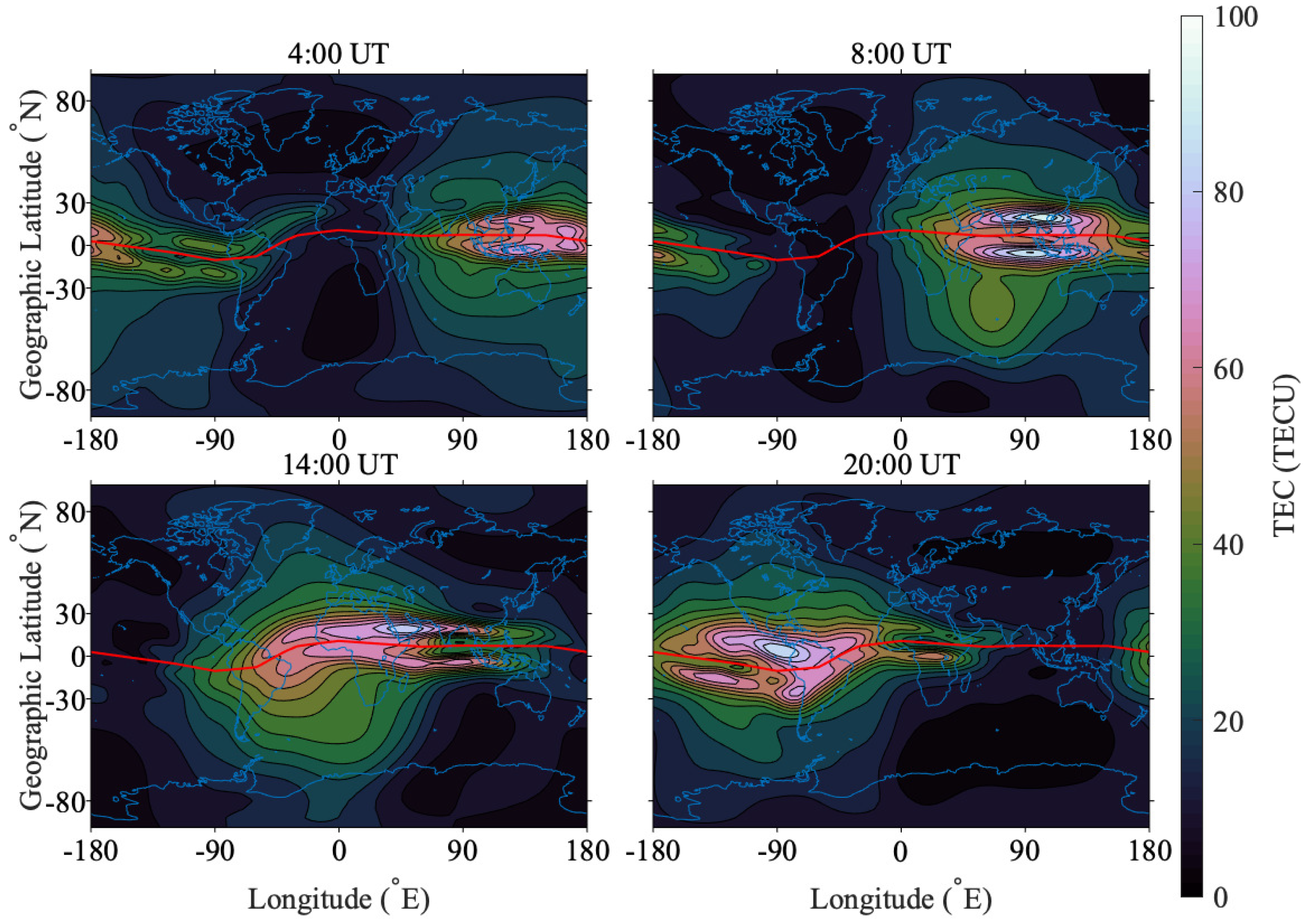
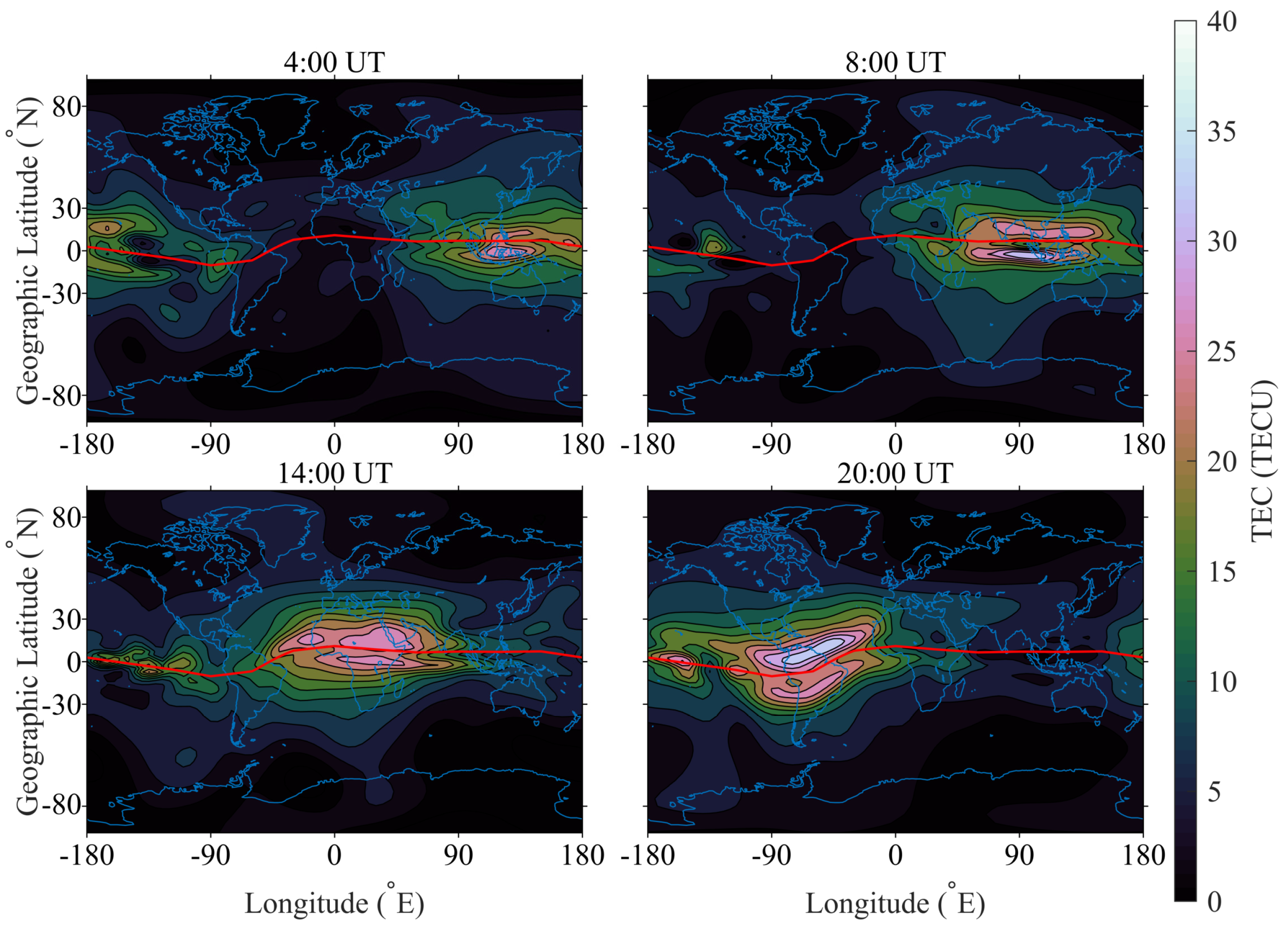
The GIMs obtained by GACI are shown in Figure 7, where the red line represents the true magnetic equator. It can be seen from the GIMs that the phenomenon of EIA is clear near the magnetic equator, and there is no obvious unreasonable value due to the use of multi-source data.

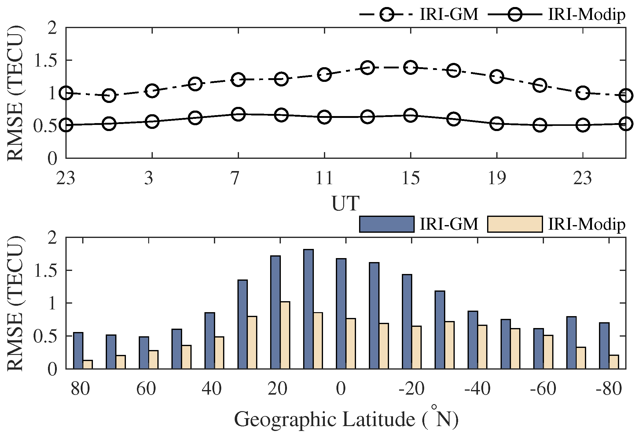
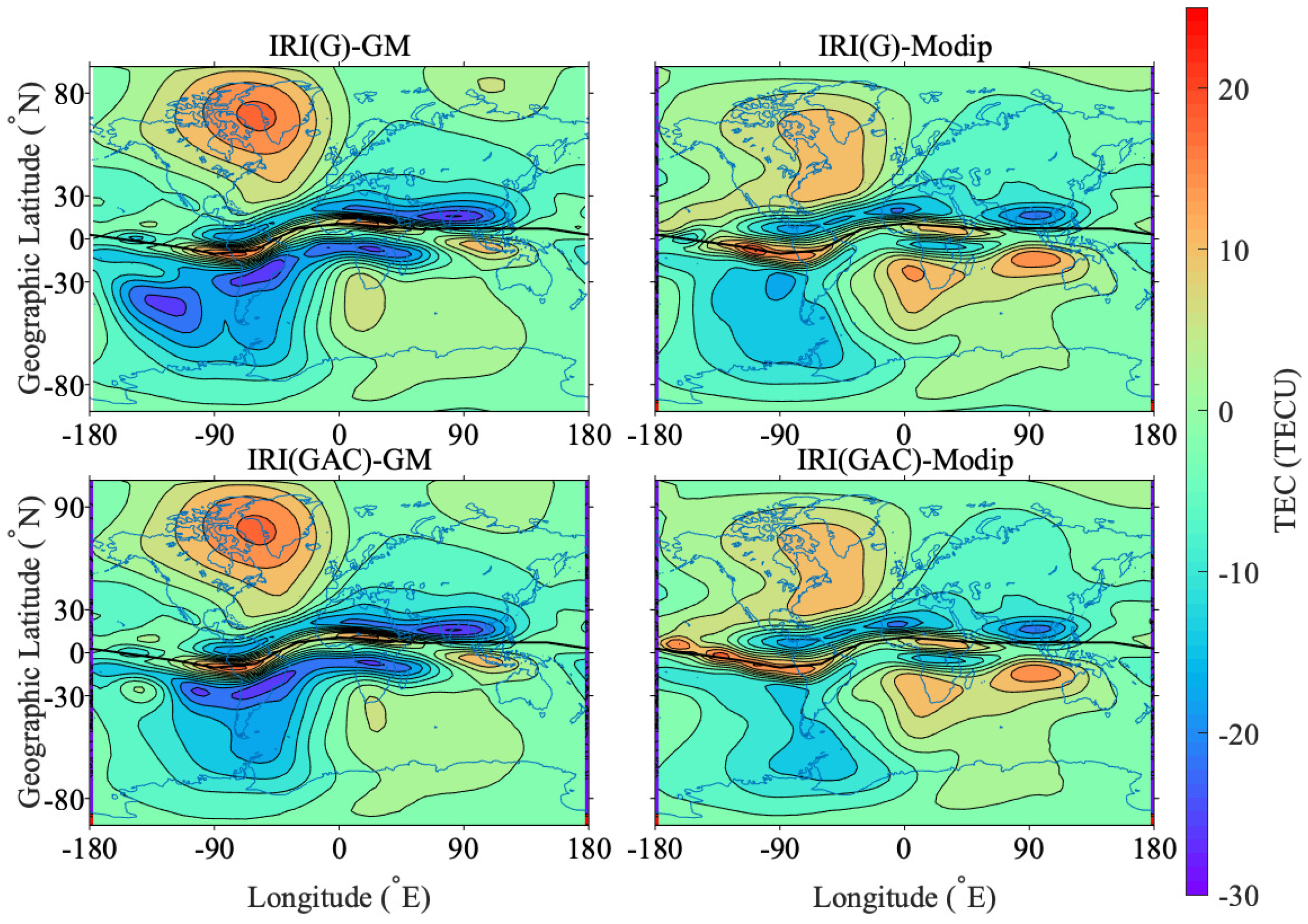
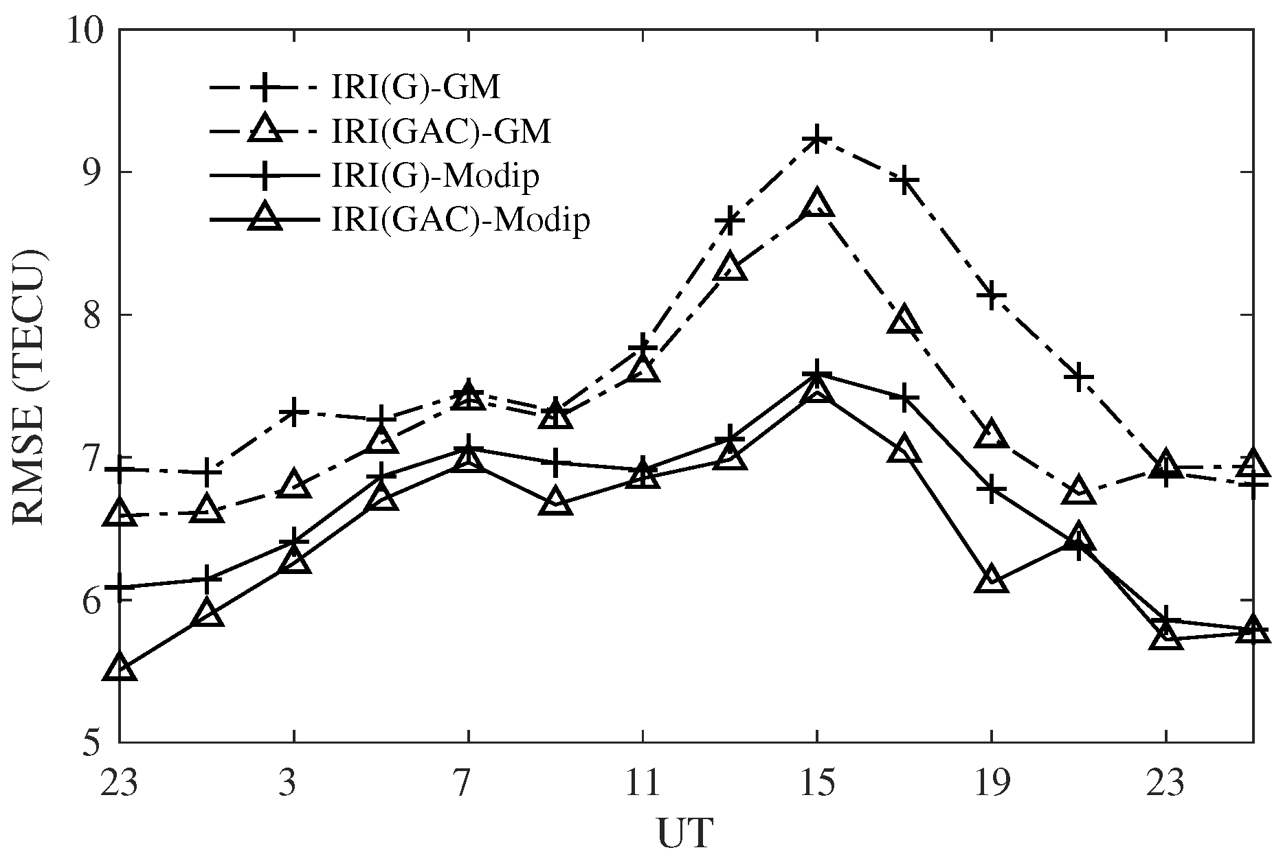
We used the data generated from the IRI model to study the impacts of the coordinate system in the global ionospheric TEC derivation in Section 3, and the conclusion remains unchanged when using the observation data, where the RMSE of the fitting residuals in different coordinate systems can be found at Figure 8. The mean improvement by using the modip latitude is about $7.02\%$ in the 12 days of geomagnetic quiet conditions in 2014, and the performances of using geomagnetic and modip reference frames in the 3 days of June are quite close, but there are obvious improvements in the 3 days of March, September and December.

In Section 3, Figure 2 shows that the main differences between the reference data with the derived values in the modip latitude mainly exist in two regions: the SAMA region and EA, which is related to the position of the EIA. The SAMA region is a place where the lowest value of the total magnetic field intensity is situated, and has a relation with equatorial electrodynamic processes [31]. To investigate the fitting situation in these areas, data from the IRI model in the area of ${20}^{\circ }$ S~${20}^{\circ }$ N in modip latitude and ${180}^{\circ }$ W~${180}^{\circ }$ E in longitude were selected, and the residuals were studied. On DOY 265, 2014, the residuals have a mean value of 6.39 TECU, which ranges from 35.85 to −19.59 TECU and has an obvious diurnal variation. The mean value of the residuals starts to increase at around 9:00 UT and reaches the maximum at 17:00 UT, which has a relation with the positions of the EA and SAMA regions. According to Figure 7, the EIA started to reach the SAMA region at around 8:00 UT, and the residual values began to increase at the same time, reaching the maximum at around 17:00–19:00 UT, which happens to be the time when the longitude of the EIA coincides with the SAMA region.

We also investigated the data for 3 days in September 2020 (DOY 264, 266, 268), which was a year of low solar activity, and the GIMs obtained by GACI on DOY 266, 2020 are shown in Figure 9. COSMIC-2 and JASON-3 were used in this calculation on the date we chose. Currently, COSMIC-2 is able to provide about 4000 radio occultations per day, which is helpful for global ionospheric mapping due to the increased number. Comparing Figure 7 and Figure 9, the TEC fluctuations decrease obviously in the year of low solar activity, the maximum value dropping from about 100 TECU to 40 TECU. In 2014, the RMSE in a global scale decreases from [2.31, 3.33] TECU in geomagnetic latitude to [1.96, 2.91] TECU in modip latitude, while in 2020, the RMSE decreases from [1.35, 1.87] TECU in geomagnetic latitude to [1.29, 1.81] TECU in modip latitude, where the mean improvements are about $8.54\%$ and $3.25\%$ in the 3 days of September in 2014 and 2020, respectively. The performance using the modip latitude is less obvious in the year of low solar activity.

4.2. Comparison of Gim with CODE

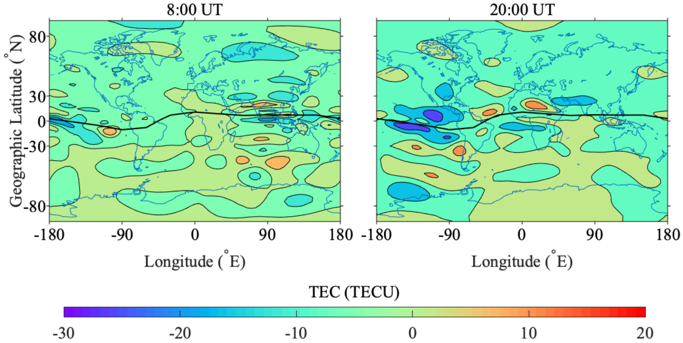
The GIMs obtained from CODE were derived by an SH function but used ground-based GNSS data and geomagnetic latitude [7]. The difference maps between GACI with CODE are shown in Figure 10, where the black line represents the true magnetic equator. The GIMs based on global basis expansions, such as the SH expansion, are more likely to be affected by the unbalanced amount of GNSS observations. The uneven IPP distribution in space distorts the inverted SH coefficients and thus is expected to affect the performance [14]. 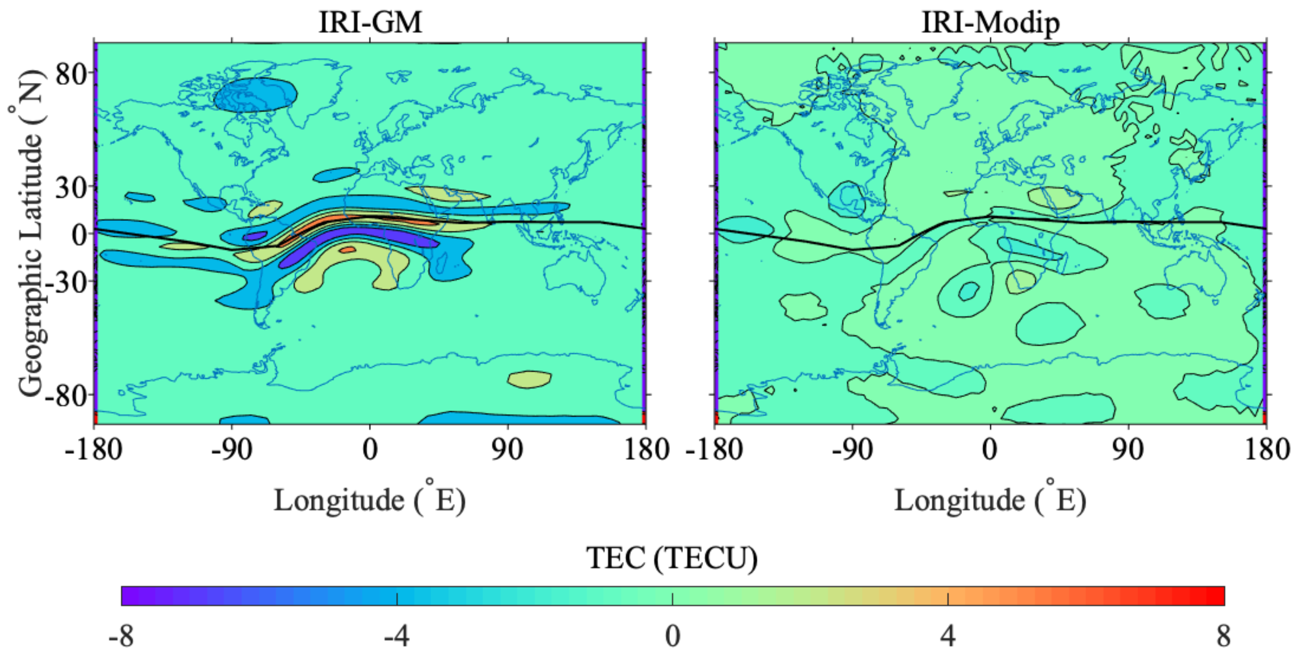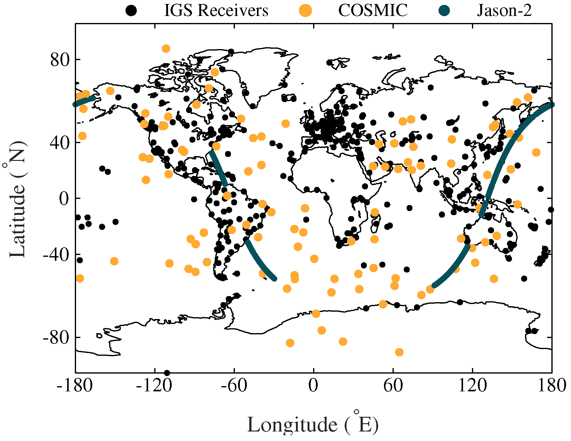From Figure 4, the uneven distribution of IGS receivers will lead to the lack of ground-based observation data in the oceanic areas, especially in the Southern Hemisphere. Compared with the GIMs from CODE, the main difference occurs near the position of the EIA, where the TEC values and the difference between modip and geomagnetic latitude are the largest, ranging from 19.42 to −25.75 TECU. The difference at 20:00 UT is larger than that at 8:00 UT, which can be attributed to the proximity of the EIA and SAMA. At oceanic regions in the Southern Hemisphere, where the ground-based observations are limited, the GIMs from GACI have a larger values about 5 TECU generally, which can result from the addition of multi-source data.

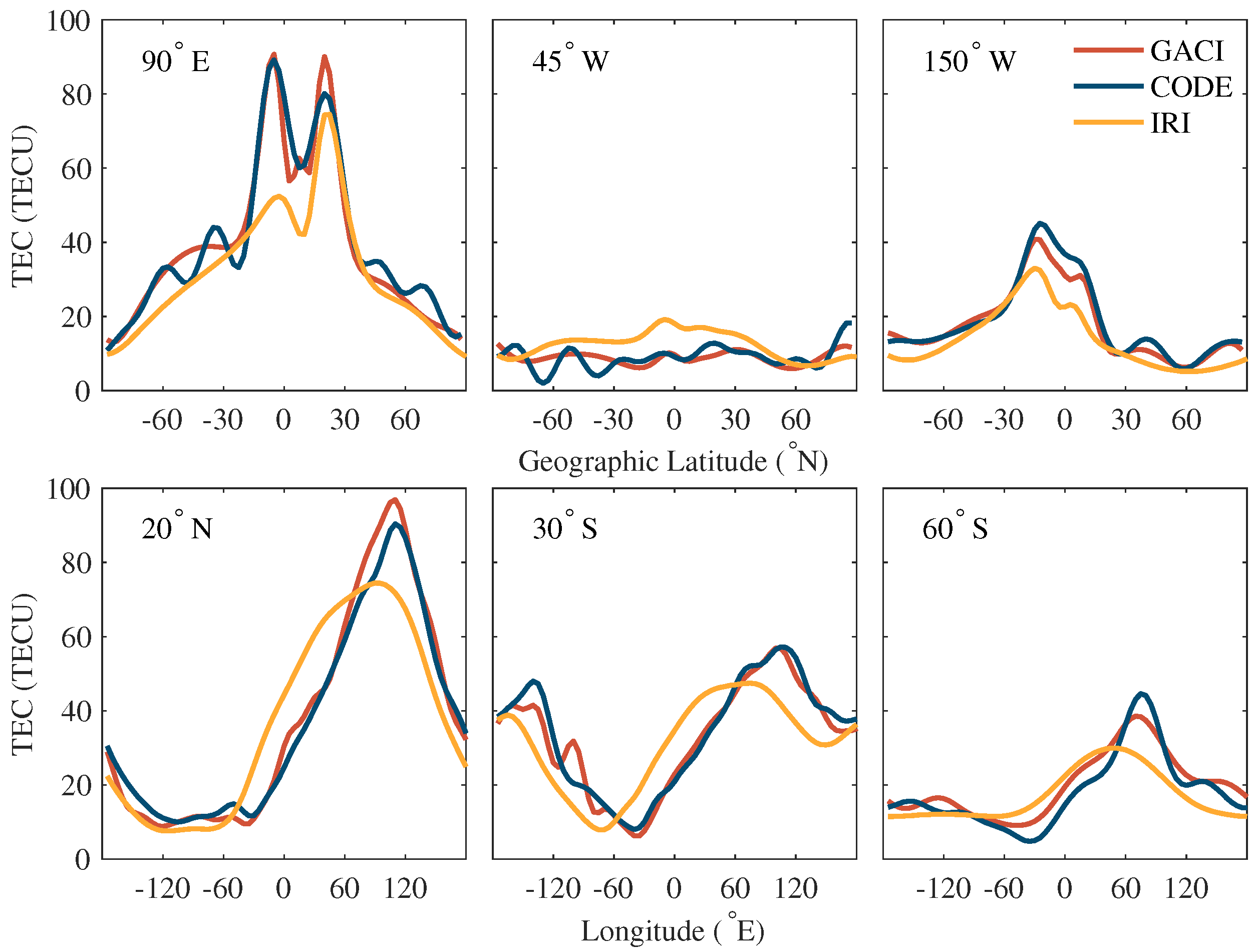
To have a clear picture of the TEC changes, especially in the areas of the EIA, SAMA and the Pacific Ocean, which lack observation data, three averaged latitudinal profiles at ${90}^{\circ }$ E, ${45}^{\circ }$ W and ${150}^{\circ }$ W and three averaged VTEC longitudinal profiles at ${20}^{\circ }$ N, ${30}^{\circ }$ S and ${60}^{\circ }$ S were extracted, the results of which are plotted in Figure 11. In addition, the profiles from GIMs of the IRI-2016 model were computed at the same epoch longitude. Similar to the conclusion we obtained earlier, the differences among GACI and CODE are more obvious in the EA and middle- and high-latitude areas of the Southern Hemisphere, where the number of observations is limited. The mean difference among GACI and CODE is less than 1.88 TECU, but has an obvious discrepancy up to 14.35 TECU in the oceanic areas of the Southern Hemisphere. GIMs obtained from the IRI-2016 of an empirical ionosphere model has a lower precision compared with GIMs from GACI and CODE, where the maximum difference value can reach about 40 TECU. However, the addition of data from the IRI model is still needed to provide ionospheric information for areas where the number of observations is limited to decrease the residual by making data evenly distributed and reduce the occurrence possibility of the unreasonable values.

4.3. Satellite Bias Estimation

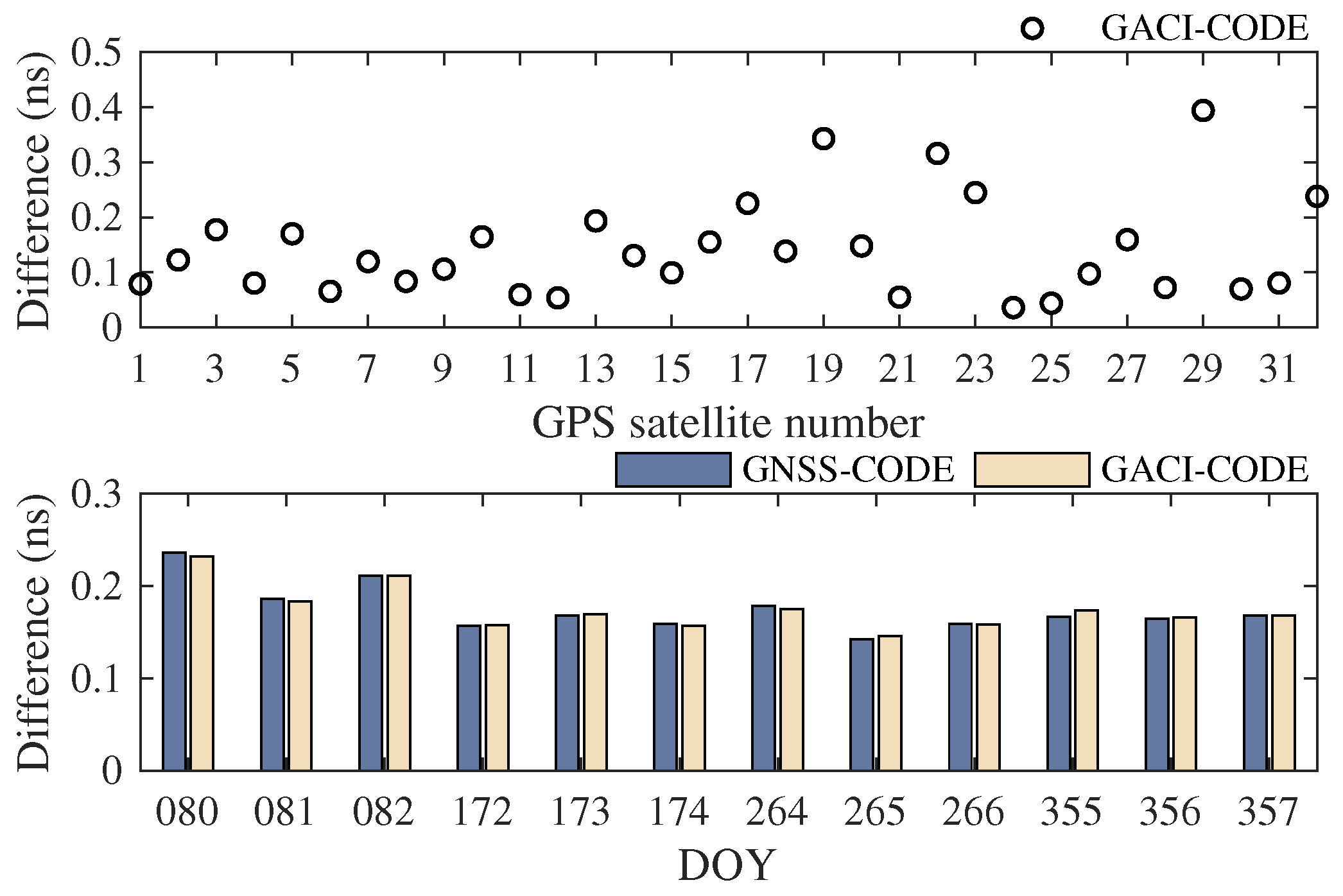
As a by-product in the TEC derivation, the DCBs of satellites and receivers can reflect the accuracy and reliability of the GIM to a certain extent. Figure 12 demonstrates the satellite DCB (P1-P2) comparison for fitting with GNSS and GACI with respect to the Center for Orbit Determination in Europe (CODE) in 2014. The difference in satellite DCBs for GACI with CODE is about 0.17 ns in the 12-day data of 2014, which can be attributed to the different observation data and coordinate systems used in CODE and GACI. In addition, the use of multi-source data exerts a limited influence on the DCB determination.

5. Conclusions

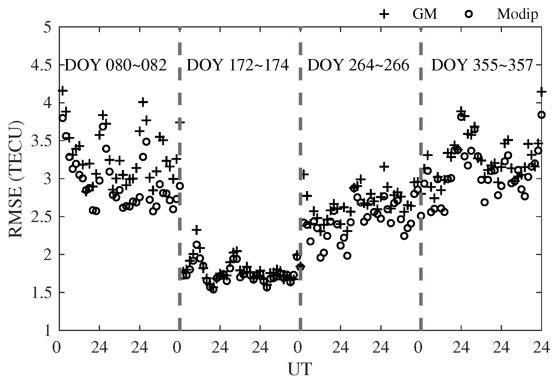
We analyzed the improvement of two aspects in global ionospheric TEC derivation: multi-source data and coordinate system. In order to have an overall understanding of these two aspects, we first generated TEC using the IRI-2016 model at a resolution of ${2.5}^{\circ }\times 5^{\circ }\times 0.1$ h in latitude, longitude and time. Simulation with the IRI model showed that the RMSE can be decreased by about $10.88\%$ when using modip latitude and multi-source data, and the improvement of adding space-based observations is about $4.49\%$ in the extrapolation areas, which have a relation to the amount of space-based data we added. Large deviations mainly occur in the EA, SAMA region and oceans where observation data is limited.

Global TEC were derived by using an SH function in modip latitude with multi-source data at a resolution of ${2.5}^{\circ }\times 5^{\circ }\times 2$ h in latitude, longitude and time. Observations from GNSS, JASON-2/3 satellite altimetry and COSMIC-1/2 occultation, and virtual observations from the IRI-2016 model, which were added at the center of each grid with no observation, were combined to derive the global ionospheric TEC, and following conclusions were made: the RMSE reduction of fitting with modip latitude had a mean value of about $7.02\%$ in the 12 days of geomagnetic quiet conditions for four seasons in 2014 when using multi-source data, and the improvement was the largest in March and smallest in June; the mean residual in the EA, where the difference is supposed to be obvious, showed a diurnal variation and reached the maximum when the positions of the EIA and SAMA are close; the improvement of using modip latitude was less obvious in the year of low solar activity; the DCB difference between GACI and CODE was about 0.17 ns, and the TEC difference was mainly at the EA and oceans, where the GIMs from GACI had a larger value of about 5 TECU in the oceanic areas of the Southern Hemisphere due to the use of multi-source data.

These results show that more satellite observations and a suitable coordinate system play an important role in global ionospheric TEC derivation. With the development of various ionospheric sounding techniques, multi-source observation data will become increasingly crucial in the obtainment of GIMs with high precision in the future.

References

1. Coco, D.S.; Coker, C.; Dahlke, S.R.; Clynch, J.R. Variability of GPS satellite differential group delay biases. IEEE Trans. Aerosp. Electron. Syst. 1991, 27, 931–938. [Google Scholar] [CrossRef]
2. Wilson, B.D.; Mannucci, A.J.; Edwards, C.D. Subdaily northern hemisphere ionospheric maps using an extensive network of GPS receivers. Radio Sci. 1995, 30, 639–648. [Google Scholar] [CrossRef]
3. Schaer, S.; Beutler, G.; Rothacher, M.; Springer, T.A. Daily global ionosphere maps based on GPS carrier phase data routinely produced by the CODE Analysis Center. In Proceedings of the IGS Analysis Center Workshop 1996, Silver Spring, MD, USA, 19–21 March 1996. [Google Scholar]
4. Hernández-Pajares, M.; Juan, J.; Sanz, J.; Orus, R.; Garcia-Rigo, A.; Feltens, J.; Komjathy, A.; Schaer, S.; Krankowski, A. The IGS VTEC maps: A reliable source of ionospheric information since 1998. J. Geod. 2009, 83, 263–275. [Google Scholar] [CrossRef]
5. Ghoddousi-Fard, R. GPS Ionospheric Mapping at Natural Resources Canada; IGS Workshop: Pasadena, CA, USA, 2014. [Google Scholar]
6. Feltens, J. Development of a new three-dimensional mathematical ionosphere model at European Space Agency/European Space Operations Centre. Space Weather. 2007, 5, 1–17. [Google Scholar] [CrossRef] [Green Version]
7. Schaer, S. Mapping and Predicting the Earth’s Ionosphere Using the Global Positioning System. Ph.D. Thesis, Bern University, Bern, Switzerland, 1999. [Google Scholar]
8. Hernández-Pajares, M.; Juan, J.; Sanz, J. New approaches in global ionospheric determination using ground GPS data. J. Atmos. Sol. Terr. Phys. 1999, 61, 1237–1247. [Google Scholar] [CrossRef]
9. Mannucci, A.; Wilson, B.; Yuan, D.; Ho, C.; Lindqwister, U.; Runge, T. A global mapping technique for GPS-derived ionospheric total electron content measurements. Radio Sci. 1998, 33, 565–582. [Google Scholar] [CrossRef]
10. Li, Z.; Yuan, Y.; Wang, N.; Hernandez-Pajares, M.; Huo, X. SHPTS: Towards a new method for generating precise global ionospheric TEC map based on spherical harmonic and generalized trigonometric series functions. J. Geod. 2015, 89, 331–345. [Google Scholar] [CrossRef]
11. Zhang, H.; Xu, P.; Han, W.; Ge, M.; Shi, C. Eliminating negative VTEC in global ionosphere maps using inequality-constrained least squares. Adv. Space Res. 2013, 51, 988–1000. [Google Scholar] [CrossRef]
12. Roma-Dollase, D.; Hernández-Pajares, M.; Krankowski, A.; Kotulak, K.; Ghoddousi-Fard, R.; Yuan, Y.; Li, Z.; Zhang, H.; Shi, C.; Wang, C.; et al. Consistency of seven different GNSS global ionospheric mapping techniques during one solar cycle. J. Geod. 2018, 92, 691–706. [Google Scholar] [CrossRef] [Green Version]
13. Alizadeh, M.; Schuh, H.; Todorova, S.; Schmidt, M. Global ionosphere maps of VTEC from GNSS, satellite altimetry, and Formosat-3/COSMIC data. J. Geod. 2011, 85, 975–987. [Google Scholar] [CrossRef]
14. Yao, Y.; Liu, L.; Kong, J.; Zhai, C. Global ionospheric modeling based on multi-GNSS, satellite altimetry, and Formosat-3/COSMIC data. GPS Solut. 2018, 22, 104. [Google Scholar] [CrossRef]
15. An, X.; Meng, X.; Jiang, W.; Chen, H.; He, Q.; Xi, R. Global Ionosphere Estimation Based on Data Fusion From Multisource: Multi-GNSS, IRI Model, and Satellite Altimetry. J. Geophys. Res. Space Phys. 2019, 124, 6012–6028. [Google Scholar] [CrossRef]
16. An, X.; Meng, X.; Chen, H.; Jiang, W.; Xi, R.; Chen, Q. Modelling Global Ionosphere Based on Multi-Frequency, Multi-Constellation GNSS Observations and IRI Model. Remote Sens. 2020, 12, 439. [Google Scholar] [CrossRef] [Green Version]
17. Laundal, K.M.; Richmond, A.D. Magnetic coordinate systems. Space Sci. Rev. 2017, 206, 27–59. [Google Scholar] [CrossRef] [Green Version]
18. Rawer, K. Meteorological and Astronomical Influences on Radio Wave Propogation; Landmark, B., Ed.; Pergamon Press: Oxford, UK, 1963; pp. 221–250. [Google Scholar]
19. Rawer, K. Encyclopedia of Physics, Geophysics III, Part VII; Springer: Berlin/Heidelberg, Germany, 1984; pp. 389–391. [Google Scholar]
20. Azpilicueta, F.; Brunini, C.; Radicella, S. Global ionospheric maps from GPS observations using modip latitude. Adv. Space Res. 2006, 38, 2324–2331. [Google Scholar] [CrossRef]
21. Teunissen, P.; Montenbruck, O. Springer Handbook of Global Navigation Satellite Systems; Springer: Berlin/Heidelberg, Germany, 2017. [Google Scholar]
22. Chen, P.; Yao, W.; Zhu, X. Combination of ground-and space-based data to establish a global ionospheric grid model. IEEE Trans. Geosci. Remote Sens. 2014, 53, 1073–1081. [Google Scholar] [CrossRef]
23. Sardon, E.; Rius, A.; Zarraoa, N. Estimation of the transmitter and receiver differential biases and the ionospheric total electron content from Global Positioning System observations. Radio Sci. 1994, 29, 577–586. [Google Scholar] [CrossRef]
24. Ma, G.; Gao, W.; Li, J.; Chen, Y.; Shen, H. Estimation of GPS instrumental biases from small scale network. Adv. Space Res. 2014, 54, 871–882. [Google Scholar] [CrossRef]
25. Ma, G.; Maruyama, T. Derivation of TEC and estimation of instrumental biases from GEONET in Japan. Ann. Geophys. 2003, 21, 2083–2093. [Google Scholar] [CrossRef] [Green Version]
26. Brunini, C.; Meza, A.; Bosch, W. Temporal and spatial variability of the bias between TOPEX-and GPS-derived total electron content. J. Geod. 2005, 79, 175–188. [Google Scholar] [CrossRef]
27. Imel, D.A. Evaluation of the TOPEX/POSEIDON dual-frequency ionosphere correction. J. Geophys. Res. Ocean. 1994, 99, 24895–24906. [Google Scholar] [CrossRef]
28. Liou, Y.A.; Pavelyev, A.G.; Matugov, S.S.; Yakovlev, O.I.; Wickert, J. Radio Occultation Method for Remote Sensing of the Atmosphere and Ionosphere; I-Tech Education and Publishing KG: Rijeka, Croatia, 2010. [Google Scholar]
29. Wang, D.; Luo, X.; Wang, J.; Gao, J.; Zhang, T.; Wu, Z.; Yang, C.; Wu, Z. Global Ionospheric Model Accuracy Analysis Using Shipborne Kinematic GPS Data in the Arctic Circle. Remote Sens. 2019, 11, 2062. [Google Scholar] [CrossRef] [Green Version]
30. Dettmering, D.; Schmidt, M.; Heinkelmann, R.; Seitz, M. Combination of different space-geodetic observations for regional ionosphere modeling. J. Geod. 2011, 85, 989–998. [Google Scholar] [CrossRef]
31. Abdu, M.; Batista, I.; Carrasco, A.; Brum, C. South Atlantic magnetic anomaly ionization: A review and a new focus on electrodynamic effects in the equatorial ionosphere. J. Atmos. Sol. Terr. Phys. 2005, 67, 1643–1657. [Google Scholar] [CrossRef] [Green Version]
Figure 1. Comparison of modip (red) and geomagnetic (blue) latitude in September 2014.
Atmosphere 12 00434 g001
Figure 2. Residual maps of fitting in geomagnetic latitude (left) and modip latitude (right) at 18:00 UT, day of year (DOY) 265, 2014.
Atmosphere 12 00434 g002
Figure 3. Root-mean-square error (RMSE) in geomagnetic and modip coordinate systems over time (top) and different latitude bands (bottom) on DOY 265, 2014.
Atmosphere 12 00434 g003
Figure 4. Locations of International GNSS Service (IGS) receivers and ionospheric piercing points (IPPs) of space-based observation data at 16:00–18:00 UT, DOY 265, 2014.
Atmosphere 12 00434 g004
Figure 5. Residual maps of fitting in different coordinate systems (18:00 UT, DOY 265, 2014).
Atmosphere 12 00434 g005
Figure 6. RMSE of fitting residual in geomagnetic and modip latitude (DOY 265, 2014).
Atmosphere 12 00434 g006
Figure 7. Global ionospheric maps (GIMs) calculated with GACI (DOY 265, 2014).
Atmosphere 12 00434 g007
Figure 8. RMSE of fitting residual with observation data in different coordinate systems in 2014.
Atmosphere 12 00434 g008
Figure 9. GIMs calculated with GACI (DOY 266, 2020).
Atmosphere 12 00434 g009
Figure 10. Differences between GIMs from GACI and the Center for Orbit Determination in Europe (CODE) at 08:00 UT (left) and 20:00 UT (right) on DOY 265, 2014.
Atmosphere 12 00434 g010
Figure 11. Averaged vertical TEC (VTEC) latitudinal profiles for GACI, CODE and IRI at 90 E, 45 W and 150 W (top), and averaged VTEC longitudinal profiles for GACI, CODE and IRI at 20 N, 30 S and 60 S (bottom) (8:00 UT, DOY 265, 2014).
Atmosphere 12 00434 g011
Figure 12. Differences in differential code bias (DCB) (P1-P2) in GACI with respect to CODE on DOY 265, 2014 (top), and DCB (P1-P2) comparison for GNSS and GACI with respect to CODE in 2014 (bottom).
Atmosphere 12 00434 g012