Article

Co-Seismic Ionospheric Disturbance with Alaska Strike-Slip Mw7.9 Earthquake on 23 January 2018 Monitored by GPS

1
College of Geodesy and Geomatics, Shandong University of Science and Technology, Qingdao 266590, China
2
School of Geodesy and Geomatics, Wuhan University, Wuhan 430079, China
3
China Earthquake Network Center, Beijing 100045, China
*
Authors to whom correspondence should be addressed.
Atmosphere 2021, 12(1), 83; https://doi.org/10.3390/atmos12010083
Submission received: 11 December 2020 / Revised: 31 December 2020 / Accepted: 5 January 2021 / Published: 7 January 2021
(This article belongs to the Special Issue Ionospheric Monitoring and Modelling for Space Weather)

Abstract

:
The Mw7.9 Alaska earthquake at 09:31:40 UTC on 23 January 2018 occurred as the result of strike slip faulting within the shallow lithosphere of the Pacific plate. Global positioning system (GPS) data were used to calculate the slant total electron contents above the epicenter. The singular spectrum analysis (SSA) method was used to extract detailed ionospheric disturbance information, and to monitor the co-seismic ionospheric disturbances (CIDs) of the Alaska earthquake. The results show that the near-field CIDs were detected 8–12 min after the main shock, and the typical compression-rarefaction wave (N-shaped wave) appeared. The ionospheric disturbances propagate to the southwest at a horizontal velocity of 2.61 km/s within 500 km from the epicenter. The maximum amplitude of CIDs appears about 0.16 TECU (1TECU = 1016 el m−2) near the epicenter, and gradually decreases with the location of sub-ionospheric points (SIPs) far away from the epicenter. The attenuation rate of amplitude slows down as the distance between the SIPs and the epicenter increases. The direction of the CIDs caused by strike-slip faults may be affected by the horizontal direction of fault slip. The propagation characteristics of the ionospheric disturbance in the Alaska earthquake may be related to the complex conditions of focal mechanisms and fault location.

1. Introduction

The deformation of the land and seafloor surface during earthquakes will cause oscillations in the total electron contents (TECs) of the ionosphere. Various detection techniques have been used to study the ionospheric anomalies since the ionospheric disturbance was first detected after the 1964 Alaska Mw9.2 earthquake in the United States [1]. In the early days, traditional monitoring techniques such as high-frequency Doppler sounders, ionosonde, and over-the-horizon radar were used to observe ionospheric disturbances [2,3,4,5]. As the global navigation satellite system (GNSS) was used for ionospheric anomaly detection, it breaks through the space-time limitations of traditional seismic monitoring techniques, and realizes direct observation of the total electron content of ionosphere in the seismic region for the analysis of ionospheric disturbance propagation features and generation mechanisms [6,7,8,9,10,11,12,13].
The TEC oscillations in the ionosphere caused by earthquakes were called co-seismic ionospheric disturbances (CIDs) [14]. A CID has a variety of propagation characteristics (such as propagation velocity, waveform and period) [15,16,17,18,19,20,21,22,23]. These propagation characteristics were different due to different focal mechanisms and fault conditions. Using global positioning system (GPS) data from the GPS Earth Observation Network, it was found that the CID propagation characteristics for the 2011 Mw9.1 Tohoku earthquake could be caused by acoustic waves generated from Rayleigh waves, acoustic waves from the epicenter, and atmospheric gravity waves from the epicenter [24,25]. However, the CID propagation velocity and range caused by the three types of wave were different. The acoustic waves generated by focal rupture usually propagate in the near field (within 1000 km) at the velocity of sound, while the acoustic waves excited by Rayleigh waves can propagate far away in a short time [26]. The CIDs caused by different disturbance sources will overlap near the epicenter and gradually separate in the far field [11]. The waveform of CIDs will be affected by co-seismic crustal movement. The CID caused by three major earthquakes in the Kuril Arc area combined with the focal mechanism found that the waveform polarity of CID is related to the polarity of vertical co-seismic crustal movement [11]. In addition, the direction was also an important feature of CID propagation [14]. The direction of the CID made it easier to follow the direction of the magnetic field in the seismic area [13] and was also affected by the rupture zone [20].
Strike-slip earthquakes mainly produce horizontal fault movement, and the vertical displacement is smaller than that of thrust faulting [6,19]. Vertical ground motion plays a major role in the formation of CID [20,27]. There were differences in CID propagation characteristics caused by strike-slip faulting and thrust faulting [28,29]. Among CIDs caused by three strike-slip earthquakes that occurred near Indonesia, the amplitude of strike-slip faults was smaller than that of earthquakes with large vertical displacements [30]. The CID waveform caused by the two strike-slip earthquakes discovered in Turkey were all N-shaped waves and propagate at a velocity greater than the velocity of sound [31]. Seismological parameters such as the horizontal displacement of the earthquake, the size of the fault, the sliding amplitude and the magnitude of the earthquake will also be crucial with the CID caused by the strike-slip faults, in the case of controlling the vertical displacement of the co-seismic crust [28]. Although the ionospheric disturbance caused by the strike-slip earthquake was found, the earthquake details and CID propagation characteristics were not combined.
This study monitors the ionospheric disturbance after the Mw7.9 Alaska earthquake on 23 January 2018 and calculated the slant total electron content (STEC) on the basis of the GPS data provided by continuously operating reference stations (CORS) in Alaska. Detailed ionospheric disturbance signals will be extracted through singular spectrum analysis (SSA), and the CID phenomenon caused by the strike-slip earthquake was analyzed. The CID propagation characteristics (including amplitude, waveform and velocity) caused by the Alaska earthquake will be discovered. The propagation direction and amplitude attenuation rate of CIDs will be further analyzed in detail, combined with the fault condition of the Alaska earthquake. The connection between the focal mechanism of the Alaska earthquake and the ionospheric response will be revealed, which will help to monitor the short-period variations in the ionosphere after the earthquake.

2. Data and Methods

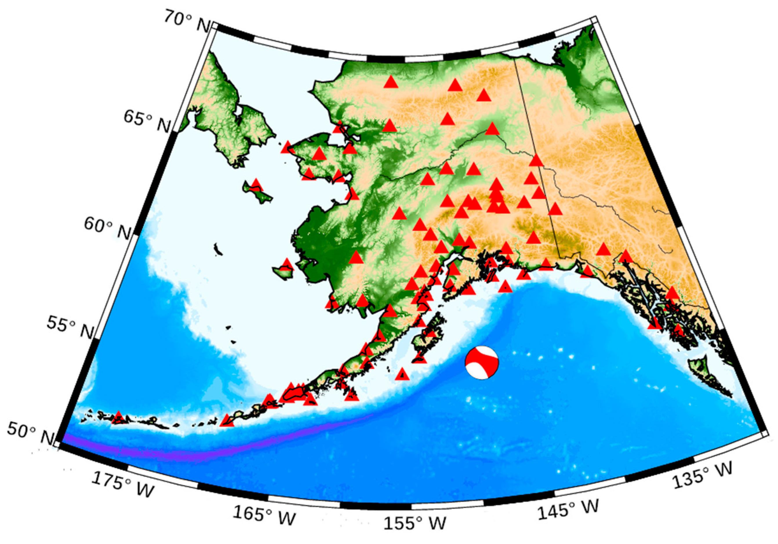
2.1. Earthquake Overview

The United States Geological Survey reported that a Mw7.9 earthquake occurred at approximately 280 km southeast of Kodiak Island in the Gulf of Alaska at 09:31:40 UTC on 23 January 2018. The epicenter was (56.004° N, 149.116° W), and the focal depth was 14.1 km. The earthquake occurred on a steeply dipping fault striking either west-southwest (left lateral) or north-northwest (right lateral) caused by strike-slip motion in the shallow lithosphere of the Pacific Plate.
The horizontal component of the seismic displacement of the Alaska seismic waveform was significantly larger than the vertical component [32]. The co-seismic displacement of the Alaska in the southwestern region of the epicenter has an upward trend from the co-seismic displacement fields released by the Navstar University Association (UNAVCO). The 2018 Mw 7.9 of Alaska Earthquake caused multiple fault ruptures, which ruptured the Pacific plate seaward of the Alaska subduction zone [33]. The largest slip of the Alaska earthquake occurred on the right-lateral south-southeast-striking (sliding amount 2.27 m) and the left-lateral northeast-striking (sliding amount 2.42 m) fault slipping segments [34].

2.2. Global Positioning System (GPS) Data

In this study, the STECs within 1 h around the seismic area of the Alaska earthquake, which are derived from the CORS GPS data at the sampling interval of 15 s, were used as the basis for detecting the CIDs after the Alaska earthquake. The CORS stations in Alaska were largely dense, providing sufficient data for subsequent research. The geographical distribution of approximately 81 CORS GPS tracking stations selected in the study is shown in Figure 1.

2.3. Solar Geomagnetic Data

The ionosphere was affected by solar and geomagnetic activity [35,36,37,38]. Solar and geomagnetic activity should be detected in the period before and after the earthquake, before extracting the ionospheric anomaly information of the Alaska earthquake. This study uses the geomagnetic index (Dst) data provided by the Geomagnetic Data Center in Kyoto, Japan, and the solar radiation index F10.7 data provided by the Space Environment Forecast Center. The Dst index was derived from the H component of the geomagnetic field and reflects the geomagnetic activity, which was normally in the range of −30~30 nT during the period of low geomagnetic activity, and the temporal resolution of the data was 1 h [39]. The solar radiation index F10.7 reflects the solar activity, which was usually less than 100 SFU (1SFU = 10−22 W m−2 Hz−1) during the period of low solar activity, and the temporal resolution for the data was 1 day [35].

2.4. Methodology

The relative change in STEC is sufficient for CID detection [39]. The equation for calculating the relative STEC using the GPS phase observation data is expressed as:
S T E C Δ = 1 40.3 f 1 2 f 2 2 f 1 2 f 2 2 ( L 1 L 2 + λ 1 N 1 λ 2 N 2 + ε )
where f 1 and f 2 are the GPS carrier frequencies, L 1 and L 2 are dual-frequency carrier phase measurements, λ 1 and λ 2 are the carrier wavelengths, N 1 and N 2 are the integer ambiguities of phase observations, and ε is the observation noise obtained from the GPS dual-frequency phase with sampling rate of 15 s. We set the cut-off elevation angle of the satellite for GPS data to 15° to calculate STEC [27].
SSA is one method for spectral decomposition [39], and can extract non-linear trends and identify periodic signals from time series, without being constrained by the assumption of sine waves [40]. Extracting seismic ionospheric disturbance signals from the relative STEC is affected by the trend and period of the TEC background caused by the orbital motion of GPS satellites and the temporal and spatial changes of the ionosphere [41,42]. SSA extracts more reliable information from data with unknown physical properties by extracting linear trend terms, identifying periods, reducing noise processing, and reconstructing time series [43]. The SSA extended empirical orthogonal function is used to extract the principal component features from the noise-containing STEC time series. The weighted correlation analysis (w-correlation) method is used to select the appropriate eigenvectors for reconstruction [41], and the remaining sequence after subtracting the reconstructed sequence is used as the STEC disturbance signals. The detailed ionospheric disturbance signals extraction steps were as follows.

2.4.1. Building the Hysteresis Matrix

The STECs at seismic period (UTC 9:00–10:00 on 23 January 2018) obtained the line of sight (LOS) between the station and GPS satellites were used as the original time series. The time series length is set to 240 under the sampling frequency of 15 s. Given a time series {x} of x 1 , x 2 , , x N , a delay matrix X is constructed as:
X = [ X 1 , X 2 , , X k ] = ( x i j ) i , j = 1 L , k = [ x 1 x 2 x N M + 1 x 2 x 3 x N M + 2 x M x M + 1 x N ]
where N is the length of the time series, and M is the nested dimension. The window length is set to one-third of the STEC data length, which is 80. We can obtain:
X i = ( x i , , x i + M 1 ) T , ( 1 i K )

2.4.2. Decomposing Singular Values

Given matrix S = X X T , where X T is the transpose matrix of X , let λ 1 , , λ M be the eigenvalue of S and U 1 , , U M is the feature vector corresponding to λ 1 , , λ M ( λ 1 λ M 0 ). Let d = r a n k ( X ) , then V i = X T U i / λ i ( i = 1 , , d ) . Delay matrix X can be expressed as:
X = X 1 + X 2 + + X d
Elementary matrix X i = λ U i V i T , r a n k ( X i ) = 1 , which has the same matrix structure as X . U and V are X left and right singular vectors, λ i ( i = 1 , , d ) is the eigenvalue of X , and { λ i } is the singular spectrum of matrix X . Considering that X 2 = i = 1 d λ i and X i 2 = λ i , we can define λ i / i = 1 d λ i as the contribution rate of elementary matrix X i , i = 1 r λ i / i = 1 d λ i and i = 1 r λ i / i = 1 d λ i as the top r contribution rate of X i .

2.4.3. Grouping

Dividing elementary matrix into { 1 , , d } disjoint subsets I 1 , I 2 , , I m ( I = { i 1 , , i p } ). The singular value decomposition (SVD) of trajectory matrix X can be expressed as: X I = X I 1 + + X I m . The group is the process of determining I 1 , I 2 , , I m .
As shown in Equation (2), we can know that the contribution rate of composite matrix X I corresponding to I can be expressed as:
κ = i I r λ i / i = 1 d λ i

2.4.4. Establishing Diagonal Average

A w-correlation method is used to analyze the correlation between reconstruction components (RCs) and grouped RCs with the same signal characteristics [44]. Assuming the obtained RC is Y i , the w-correlation of any two RC can be expressed as:
ρ i , j ω = ( Y ( i ) , Y ( j ) ) Y i ϖ Y j ϖ , ( 1 i , j N )
where Y i ϖ = ( Y ( i ) , Y ( i ) ) ( Y ( i ) , Y ( j ) ) = k = 1 N ϖ k y k i y k j , and ϖ k is the weight coefficient, which is defined as ϖ k = min ( k , M , N k ) .
When the w-correlation of the two RCs is close to one, indicating that the two RCs are more correlated. The matrix obtained by grouping is transformed into a series of new time series with a length of 240. A time series of length 240 is defined as the RCs, and the original sequence is the sum of all RCs. Z = X I k ( z 1 , z 2 , z N ) is defined as the sequence obtained by Z diagonal averaging, and let M = min ( M , K ) , K = max ( M , K ) and N = M + K 1 . z i j = z i j when M < K , otherwise z i j = z j i . The equation for diagonal averaging can be expressed as:
z i = { 1 i m = 1 k z m , i m + 1 1 i < M 1 M m = 1 L z m , i m + 1 M i K 1 N i + 1 m = i K + 1 N K + 1 z m , i m + 1 K < i N

2.4.5. Obtaining the Disturbance Signal

The l RCs and corresponding feature vector λi (1Il) obtained through SVD and eigenvalues λ k of the RCs are arranged in accordance with size λ 1 λ 2 λ l 0 . The feature vector corresponding to the magnitude of the eigenvalue represents the magnitude of the change trend of the TEC signal. The cumulative contribution rate of the eigenvalues of the first five RCs obtained using Equation (3) exceeds 95%. The first five large eigenvalues are intercepted and sorted, and the corresponding sum of χ k is found and reconstructed to fully reflect the overall characteristics of the original TEC sequence, which can be expressed as:
S T E C m a i n = 1 l R C k , ( 1 k l )
The reconstructed STEC time series main component S T E C m a i n containing the ionospheric short-period signal is used as a high-precision background reference value to extract the disturbance signal.
S T E C m a i n is subtracted from the original STEC time series to obtain the preliminary ionospheric STEC disturbance signal:
Δ S T E C = S T E C S T E C m a i n

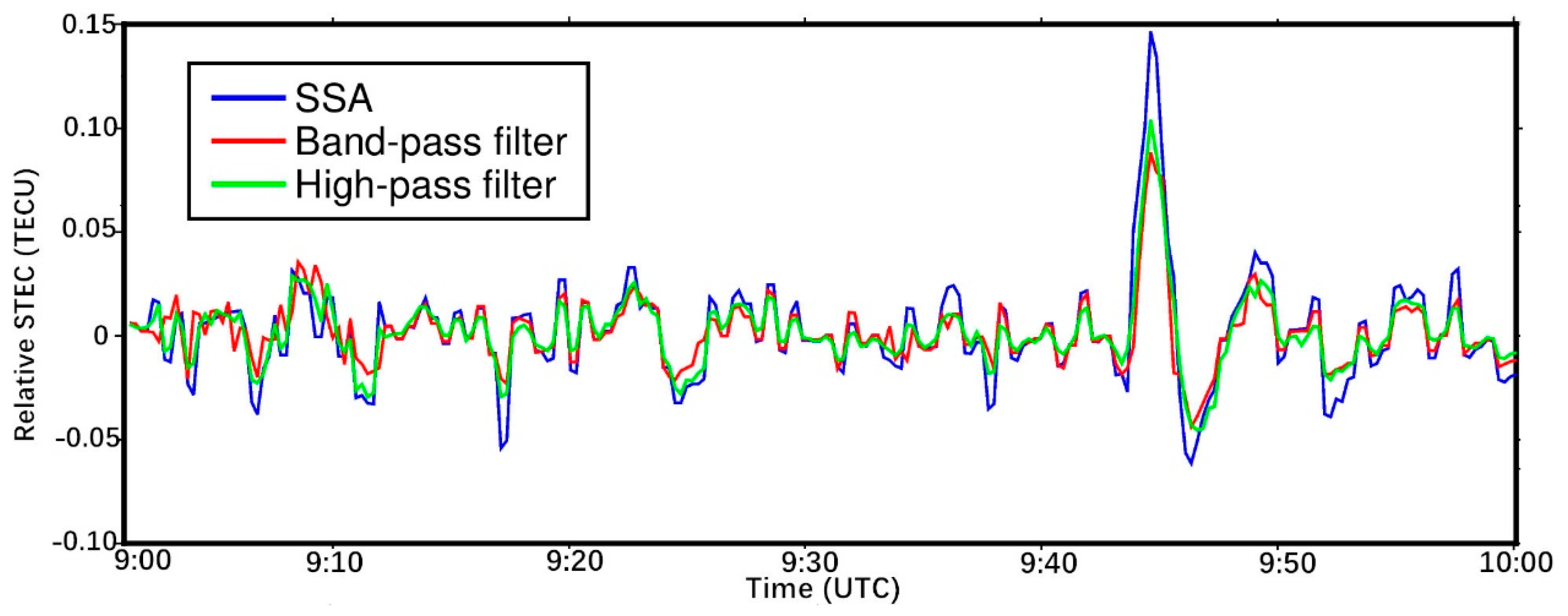
2.4.6. Eliminating Noise

The preliminary STEC disturbance signal obtained is then processed by the above steps 1–5, and the component with small contribution rate is eliminated as noise. Fifteen eigenvectors with larger eigenvalues are extracted to construct a time series as the extracted STEC disturbance signal.
The CID amplitude caused by strike-slip earthquake is small [29,30,31]. The detailed information of CID propagation characteristics caused by strike-slip earthquakes is difficult to extract. The disturbance information of the time series extracted by filtering will leak the signal, causing signal loss when extracting the CID with small amplitude. We use SSA to process the time series to retain more details of the disturbance signal and to analyze the details of CID features caused by the strike-slip earthquake. Figure 2 shows the ionospheric disturbance information along LOS between the station av07 and GPS satellite 05 extracted by the SSA, band-pass filter (cutoffs of 2 mHz and 8 mHz) [28,45], and high-pass filter (cutoff of 2 mHz) [11,14]. The features of ionospheric disturbance extracted by SSA and band-pass filter were more detailed, and the signal processed by high-pass filter causes greater changes. The ionospheric disturbance peak amplitude extracted by SSA is larger than that extracted by band-pass filter and high-pass filter, and the signal amplitude extracted by the band-pass filter is very small. The detailed ionospheric disturbance information extracted by SSA helps to analyze the details of CID propagation characteristics.

3. Results

3.1. Solar-Geomagnetic Activity Analysis

The changes in the geomagnetic D st index and solar radiation F10.7 for 10 days (18–27 January 2018), including the earthquake day. The solar radiation index F10.7 is less than 80 SFU, indicating that the solar activity is low during this period. The variation range of the geomagnetic index D st is | D st | < 25, indicating that the geomagnetic field is relatively quiet. The solar-geomagnetic activity was low on the earthquake day, and would not cause strong ionospheric disturbances.

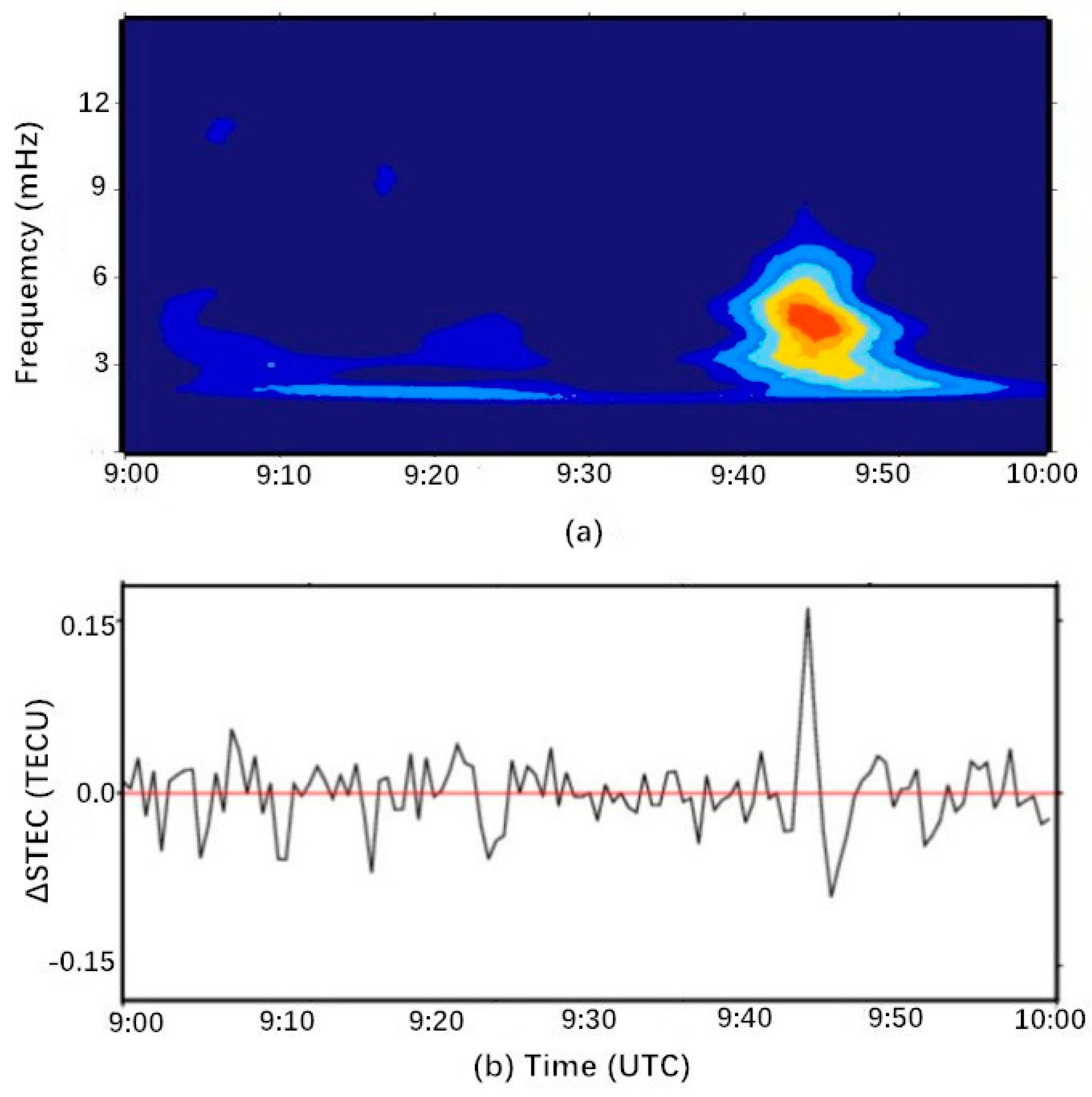
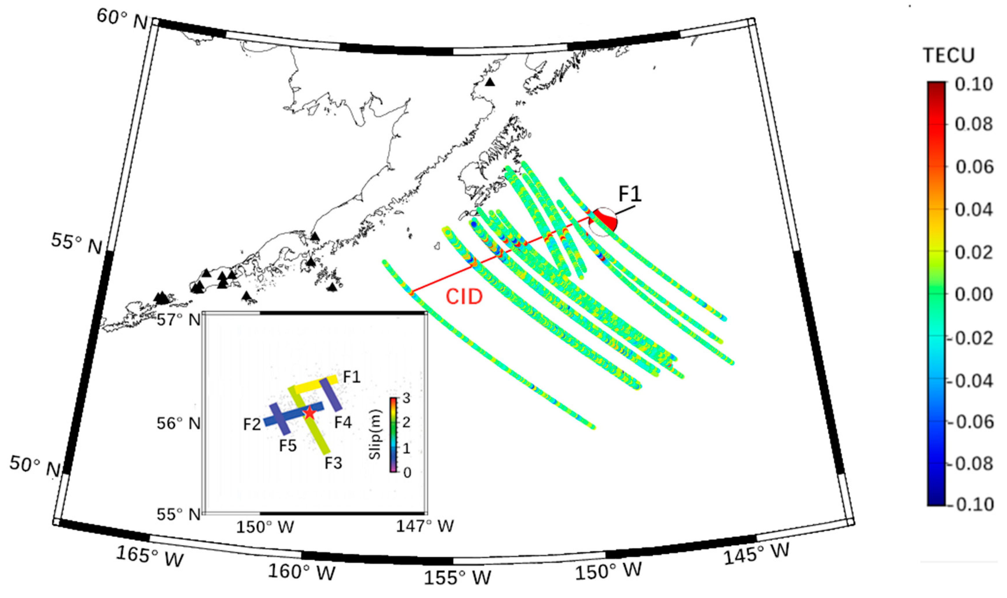
3.2. Total Electron Content (TEC) Anomalies Following the Alaska Earthquake

Based on the GPS data from CORS stations in Alaska, the disturbances of the ionosphere over the epicenter and surrounding areas during 9:00–10:00 UTC on 23 January 2018 was extracted. The height of the ionospheric shell model was given the height of the hmF 2 which was calculated as 300 km by IRI2016 model [8]. Then, the location information of CIDs calculated by the ionospheric shell model was used to analyze the CID propagation characteristics. The coordinates of ionospheric pierce point, which were the intersection of line from the satellite receiver to the thin layer, were calculated, and the epicenter distances of its corresponding sub-ionospheric point (SIP) were obtained.
Figure 3 shows the information along LOSs between the stations near the epicenter and all the GPS satellites (02, 05, 25, 29, and 31) used for the analysis covered the ionospheric area around the epicenter during 9:00–10:00 UTC.
We combine the location and time information of ionospheric anomalies recorded to determine the CID associated with the earthquake. In the information along LOS between the stations and GPS satellites (05 and 25) during 9:00–10:00 UTC on the earthquake day, CID was found above the epicenter and southwest. Figure 4 shows the time series related to the earthquake show typical “N”-shaped disturbances, appearing 8–12 min after the shock with amplitudes of 0.16 TECU (1TECU = 1016 el m−2). The time series along LOS between the station av07 and the GPS satellite 05 is taken as an example for detailed analysis of TEC response. The disturbances began at 9:38 UTC, and the first peak occurred at 9:44 UTC with amplitude of 0.14 TECU, and the distance between SIP and the epicenter was 168 km. After a few minutes, a second peak occurred at 9:48 UTC with amplitude of 0.05 TECU, and the distance between SIP and the epicenter was 162 km. The disturbance lasted for approximately 15 min, and the ionosphere gradually recovered after 9:53 UTC. The CID propagation characteristics were similar to the 2006 Mw8.2 Kuril earthquake in northeast Japan, showing typical compression-rarefaction wave (N-shaped waves) caused by co-seismic vertical crustal movements [11]. The typical waveform of CID may be related to the co-seismic vertical ground motion in the southwest of the epicenter of the Alaska earthquake [34]. The co-seismic vertical crustal movement caused by a strike-slip fault was smaller than the thrust earthquake of the same magnitude [23,29]. Although the co-seismic vertical displacement amplitude of strike-slip faults is small, it can still affect the CID waveform.

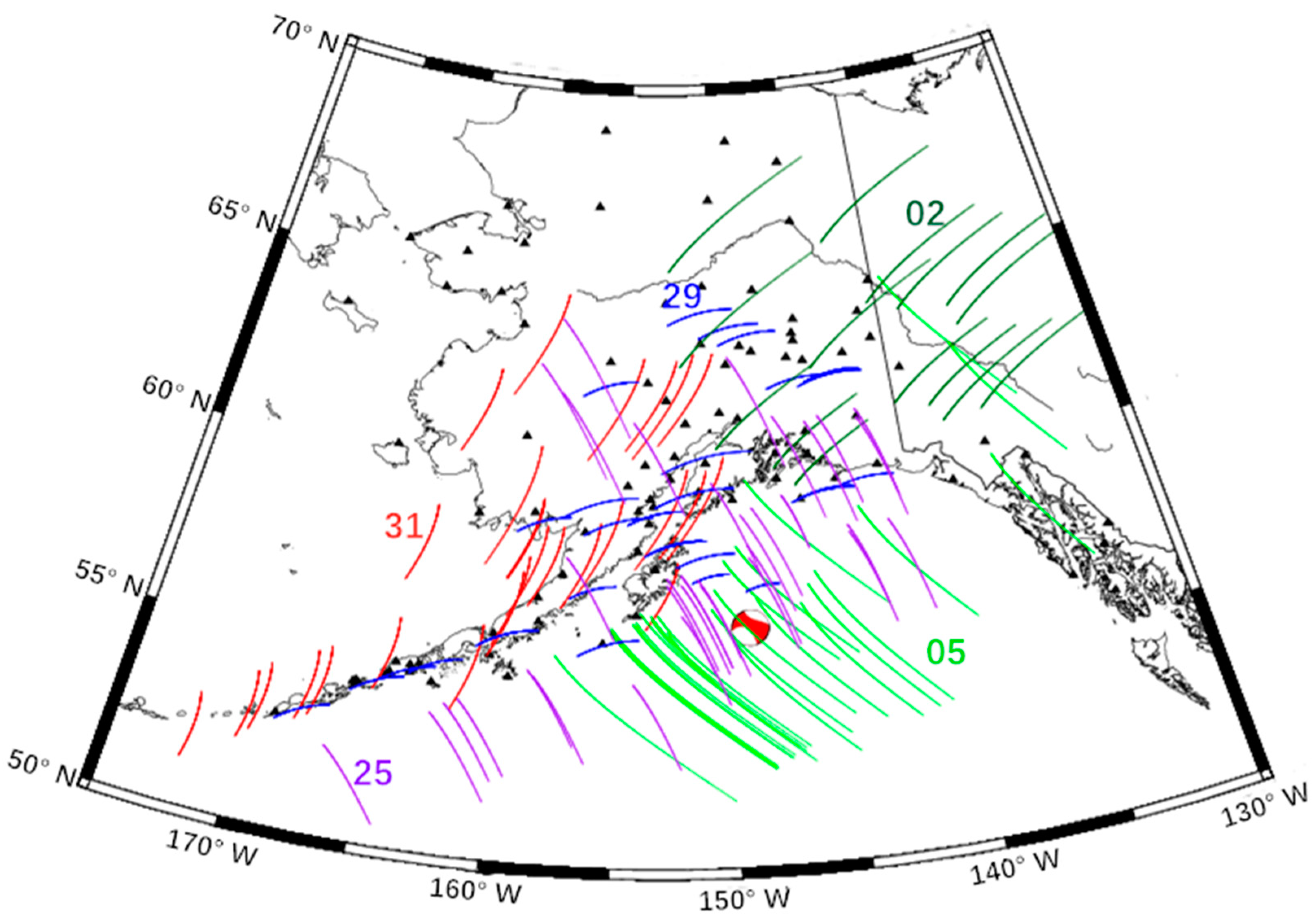
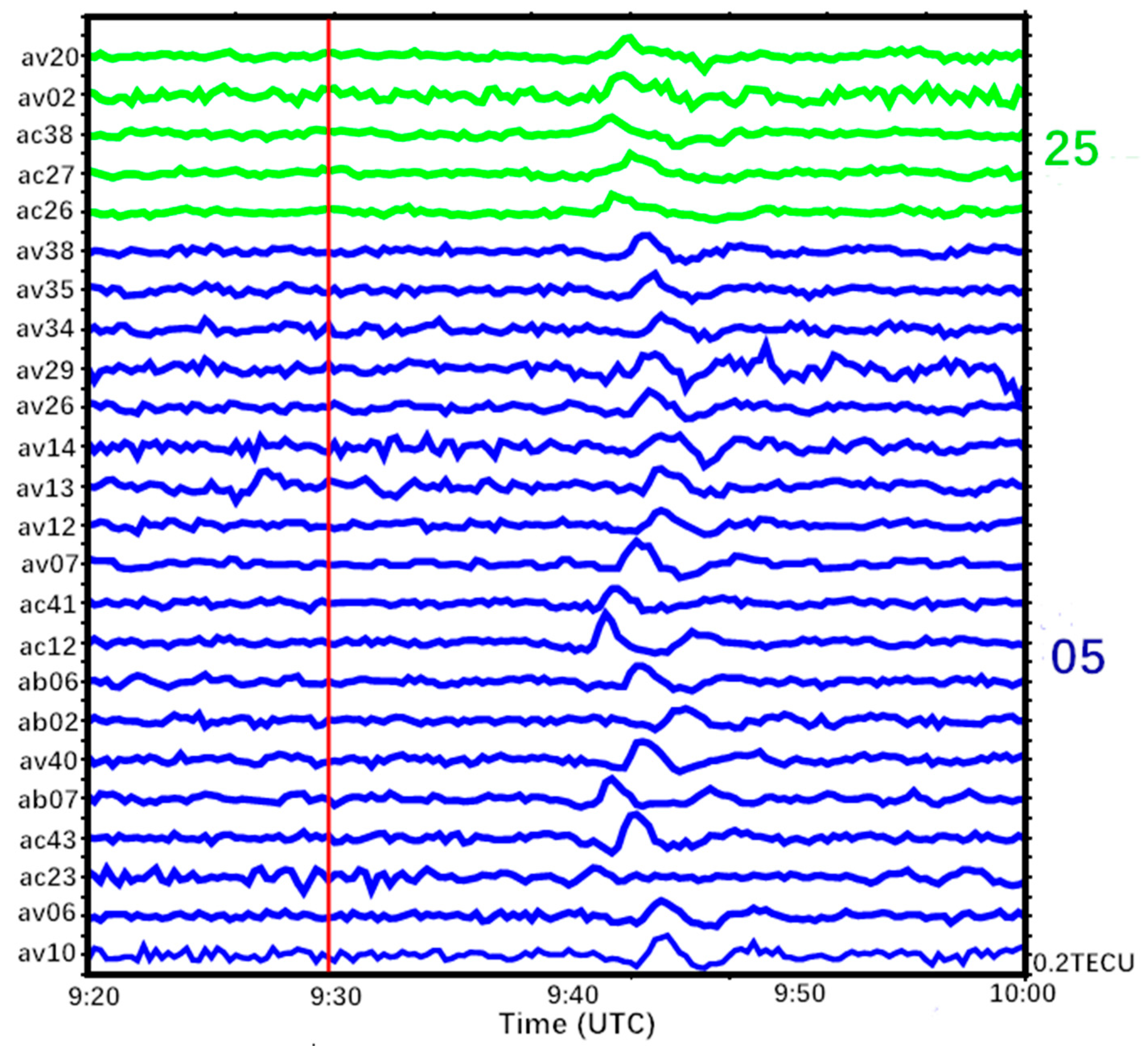
3.3. Velocity of Co-Seismic Ionospheric Disturbance (CID)

When the earthquake’s fault was located on the seafloor, the near-field CID was induced by acoustic gravity waves (AGWs) and internal gravity waves (IGWs) [11,14,31,46]. The observed frequency of ionospheric disturbances caused by gravity waves is 1–2 mHz, and the frequency of ionospheric disturbances caused by acoustic waves is 3–5 mHz [24,26]. The Pacific Tsunami Warning Center issued a tsunami warning after the Alaska earthquake, using frequency to identify ionospheric disturbances caused by IGWs and AGWs [10,21,47].
Figure 5 shows the sequence and the corresponding spectrum diagram obtained by the av07 station to the GPS satellite 05. The perturbation signal was transformed from the time domain to the frequency domain for spectral analysis using wavelet transform to determine the frequency of the time series. At the time when the abnormal value appears in the time series, the peak frequency distribution at the corresponding time in the spectrum diagram is evident, and the peak frequency of 4.8 mHz is consistent with the atmospheric resonance frequencies caused by the upward propagation of acoustic waves [24,26,48].
The horizontal propagation velocity of the CID can be calculated on the basis of the occurrence time of the CID and the epicenter distance of the SIP. Figure 6 shows the distance-time diagram of post-seismic TEC disturbances following the Alaska earthquake. A linear fit was performed using least squares in accordance with the occurrence time and the corresponding position of the CID peaks, and the slope was approximately equal to the CID propagation velocity after the earthquake.
Figure 6 shows that CIDs propagate at a certain velocity, and the amplitude decreases with time and distance between peaks and the epicenter. The propagation velocity of CID is 2.61 ± 0.06 km/s, which is much higher than the propagation velocity of acoustic waves from the epicenter and slightly lower than the horizontal propagation velocity of Rayleigh waves after the earthquake [47]. The velocity of CID was similar to the velocity of near-field CID caused by Rayleigh waves, such as the 2.2 km/s in the 2004 Mw8.1 Macquarie Island earthquake [28] and the 2.22 km/s in the 2012 Mw7.8 Haida Gwaii earthquake [49,50]. The difference in velocities can be attributed to the elevation angle and direction of the GPS satellite corresponding to the LOS [19], which is more obvious near the epicenter.
The solar-terrestrial environment is low in the period. The frequency of CID conforms to the frequency of atmospheric resonance caused by the upward propagation of acoustic waves [24,26], so we can infer that the ionospheric disturbances during this period were caused by the acoustic waves. There were two types of CID disturbance caused by acoustic waves; that is, the acoustic waves generated from Rayleigh wave, and acoustic wave effect of the focal rupture from the ionospheric epicenter. The horizontal velocity of CID caused by Rayleigh waves is close to the propagation velocity (2–4 km/s) of Rayleigh waves that usually exist in the near field [10,11,28,51]. The surface Rayleigh wave group velocity from the bottom pressure in Alaska was estimated to be approximately 2.7 km/s in the southwest directions [45], which was close to the CID velocity. These results indicate that the CID of the Alaska earthquake may be caused by the acoustic waves generated by Rayleigh waves.

3.4. CID Direction Caused by Strike-Slip Fault

Figure 7 shows the detected ionospheric anomalies and SIP trajectories. The CIDs are distributed in the southwest region within 500 km of the epicenter. The CID propagation of the Alaska earthquake showed evident directional differences, propagating from the epicenter to the southwest. The difference in CID propagation direction was mainly affected by two aspects. On the one hand, the CID propagation was affected by the earthquake rupture zone [20]. On the other hand, as the geomagnetic field makes the plasma tend to move freely along the field lines, the CID in the northern hemisphere has a trend spreading south [13].
Strike-slip fault-dominated earthquakes have a smaller rupture magnitude than thrust earthquakes, and horizontal slip is the main source of displacement [28]. The detailed horizontal slip segment of the Alaska earthquake was used to analyze the propagation characteristics of the CID. Figure 7 shows that the horizontal propagation direction CID of the Alaska earthquake was consistent with the west-southwest direction of maximum slip segment F1. Co-seismic displacement is particularly important to the generation of CID, and the maximum co-seismic displacement of the Alaska earthquake is caused by the slip segment F1 [34]. The CID spread to the south of the epicenter due to the effect of the geomagnetic field on the plasma [13]. These results indicate that the propagation of the CID in the southwest direction was not only affected by the geomagnetic field, but may also be related to the horizontal sliding direction of the fault. The CID caused by the other main sliding segment F3 was not detected during 9:30–10:00 UTC. This may be due to the fact that the CID has a tendency to spread southward due to the influence of the geomagnetic field and the direction of the sliding segment F3, while the distribution of SIPs in the south of the epicenter was lacking within half an hour after the Alaska earthquake. The CID direction of earthquakes dominated by strike-slip faults may be affected by the horizontal sliding direction of the fault.

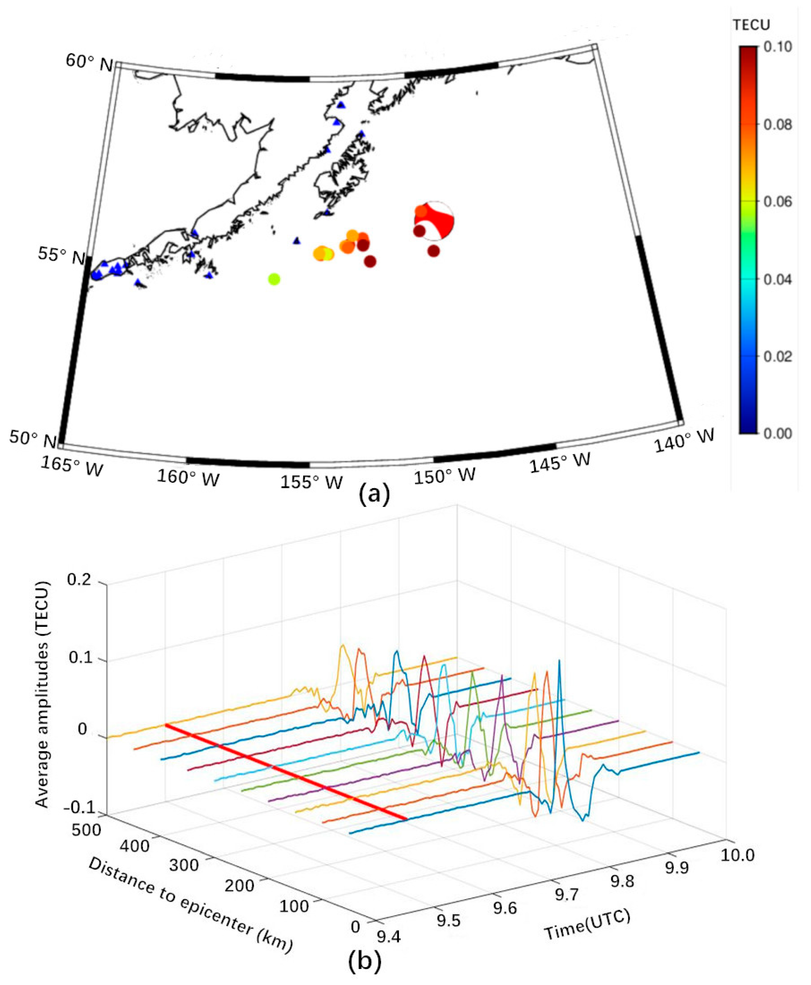
3.5. Change of CID Amplitudes

Figure 8a shows the location of the CID peaks. As the CID propagates from the epicenter to the southwest, the amplitude changes with the time and the distance between SIPs and the epicenter. The largest ionosphere disturbance was located near the epicenter as 0.16 TECU, the amplitude decreases during the propagation process, and the amplitude decreases to 0.05 TECU in the region far from the epicenter.
In the lithosphere beneath the oceans, the infrasonic acoustic waves which are generated by the vertical ground motion of seismic waves are emitted into the atmosphere and excite the acoustic waves to propagate upward to the ionosphere [9]. Due to the attenuation of atmospheric density, the ionospheric disturbance caused by acoustic waves will be amplified when acoustic waves propagate upward to the ionosphere [12,26,45]. The near-field CID amplitudes caused by the Alaska earthquake were extremely small, which was related to the small co-seismic vertical displacement caused by strike-slip faults [28,29]. The near-field CID amplitude caused by the Alaska earthquake decreases rapidly. The characteristics of rapid amplitude attenuation were similar to the near-field CID caused by Rayleigh waves in the Mw8.1 2004 Macquarie Island earthquake [28] and the 2012 Mw7.8 Haida Gwaii earthquake [50]. It may be due to the attenuation of seismic wave amplitude caused by fluid sliding in the cracks as seismic waves propagate on the surface of the medium on the seabed [52,53,54].
We use the relative value of the processed TEC to calculate the amplitude attenuation rate of the ionospheric disturbance. Figure 8b shows the relationship between the average amplitude of the CIDs and the time and distance between the SIP’s location and the epicenter. The amplitude of the CID within 200 km from the epicenter decreases at a faster rate. From 200 to 500 km, the amplitudes attenuation rate becomes slower. These characteristics were similar to the long-distance propagation features of CID found in the 2011 Mw9.1 Tohoku earthquake [55,56,57]. We found that the amplitude attenuation rate of CID decreases with increasing distance [58], not only in the CID with a longer propagation distance, but also in the near-field CID.

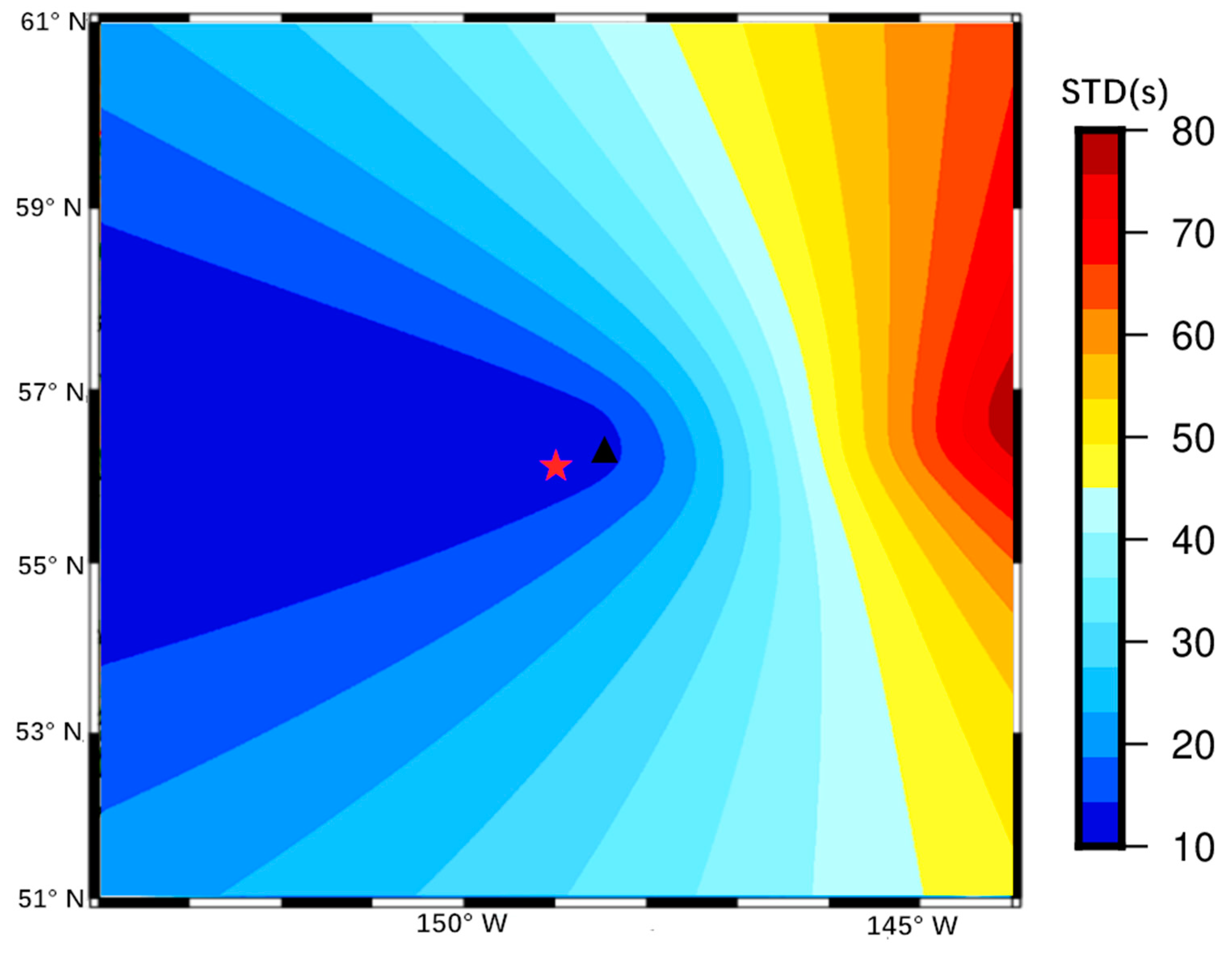
3.6. Determining the CID Source Location

The source location was determined by selecting a known CID and using ray tracing technique [19]. The ray tracing technique assumes that the seismic wave propagates to the height of the ionosphere in the vertical direction and then propagates around the horizontal direction at the velocity of the CID. From the given velocity model, the CID origin position was calculated from the CID position and velocity information. The search range of the CID source was given between 50°–60° N, 140°–155° W. At a given horizontal propagation velocity V H of the CID, an offset of 0.1° × 0.1° was used as the assumed CID source location, and the occurrence time of the CID source was expressed as [19]:
T C K = T A K ( D V K / V Z + D H K / V H )
where T A K is the observation time when the CID peak points (the first peak of each CID) appears, D V K is 300 km of the ionosphere height, V Z is the vertical velocity, and D H K is the horizontal distance from the peaks to the CID source. The CID points detected by the Alaska earthquake were used to calculate the standard deviation (STD) of the earthquake occurrence time of the grid points. The grid point with the smallest STD can be regarded as the CID source location.
Figure 9 shows that the CID source position was 56.4° N, 148.9° W, which was approximately located in the northeast of the epicenter at 47 km. The calculation of the CID source shows that the CID source was close to the location of the left-lateral northeast-striking slip segment, and both were located in the northeast direction of the epicenter. The upwardly propagating sound waves are affected by the horizontal neutral wind in the ionosphere, causing the estimated position of the CID source to be different from the actual position of the fault-sliding segment [19].

4. Conclusions

Based on the TEC calculated from GPS data, the ionospheric disturbances after the Alaska earthquake were monitored. The detailed ionospheric disturbances were extracted with SSA from the STEC data. We analyzed the propagation characteristics of the Alaska earthquake dominated by strike-slip faults, including waveform, velocity and amplitude attenuation. By analyzing the propagation characteristics of CID, it is found that the ionospheric disturbance after the earthquake may be related to the complex conditions of focal mechanisms and fault location.
The CID of the Alaska earthquake show typical “N”-shaped disturbances, appearing 8–12 min after the shock with amplitudes of 0.16 TECU. The waveform of CID may be related to the co-seismic vertical displacement in the southwest of the epicenter of the Alaska earthquake. The spectral analysis showed that the center frequency at the time of anomaly was 4.8 mHz, which was consistent with the atmospheric resonance frequencies. The propagation velocity of CID was southwestward to the distance of approximately 500 km with the horizontal phase velocity of 2.61 ± 0.06 km/s. The CID of the Alaska earthquake may be caused by the acoustic waves generated from the Rayleigh wave. The propagation direction of the CID of the Alaska earthquake was consistent with the direction of the largest slip segment. The CID direction caused by strike-slip faults was not only affected by the rupture zone and the geomagnetic field, but also by the horizontal sliding direction of the fault. As the distance between SIPs and the epicenter increases, the amplitude attenuation and the attenuation rate becomes slower. This may be related to the amplitude attenuation of seismic waves propagating on the seafloor. The location of the CID source was close to the left-lateral northeast-striking slip segment, and the propagation direction of CID may be related to the direction of sliding fault segment.
We analyzed the CID propagation characteristics of the Alaska earthquake and discovered the effect of fault location on ionospheric disturbance propagation. The rapid attenuation characteristics of the amplitude of the Alaska earthquake CID were similar to the 2011 Mw9.1 Tohoku earthquake. The CID caused by the strike-slip fault in the 2002 Mw7.9 Denali earthquake in Alaska, propagated to 3000 km with the small amplitude of 0.05 TECU. The difference in amplitude attenuation rate and range of CIDs caused by the 2018 Mw7.9 Alaska earthquake may be related to the coupling differences of the lithosphere with atmosphere in the different fault slip (inland or seabed).
This study found the connection between the detailed focus mechanism and the characteristics of CID propagation, and showed the potential for inferring the focus mechanism based on GPS data monitoring ionospheric disturbances over the epicenter. In the future, higher precision TEC data will help improve the accuracy of ionospheric disturbance monitoring. Moreover, monitoring the attenuation of the CID amplitude caused by the Alaska earthquake helps to understand the coupling mechanism between the lithosphere and the atmosphere.

Author Contributions

Conceptualization, J.G. and Y.Z.; methodology, J.G.; software, Y.Z. and K.S.; validation, Y.Z., X.L. and M.Z.; formal analysis, Y.Z.; investigation, K.S.; resources, X.L.; data curation, F.W.; writing—original draft preparation, Y.Z.; writing—review and editing, J.G. and Y.Z.; visualization, F.W.; supervision, X.L.; project administration, J.G.; funding acquisition, J.G. and X.L. All authors have read and agreed to the published version of the manuscript.

Funding

This research was funded by the National Natural Science Foundation of China (Grant Nos. 41774001, 41374009) and the SDUST Research Fund (Grant No. 2014TDJH101).

Institutional Review Board Statement

Not applicable.

Informed Consent Statement

Not applicable.

Data Availability Statement

Publicly available datasets were analyzed in this study. The CORS GPS data can be found here: [ftp://data-out.unavco.org/pub/rinex/obs/]. The geomagnetic index data can be found here: [http://wdc.kugi.kyoto-u.ac.jp/dstae/index.html]. The solar radiation index F10.7 data can be found here: [http://www.sepc.ac.cn/F107Index_chn.php]. The co-seismic displacement fields data can be found here: [ftp://data-out.unavco.org/pub/products/event/].

Acknowledgments

We are very grateful to UNAVCO for providing the GPS data and the co-seismic displacement fields, the Geomagnetic Data Center in Kyoto, Japan for providing the geomagnetic index, and the Space Environment Forecast Center for providing the solar radiation index F10.7 data.

Conflicts of Interest

The authors declare no conflict of interest.

References

  1. Leonard, R.S.; Barnes, R.A. Observation of ionospheric disturbances following the Alaska earthquake. J. Geophys. Res. 1965, 70, 1250–1253. [Google Scholar] [CrossRef]
  2. Davies, K.; Baker, D.M. Ionospheric effects observed around the time of the Alaskan earthquake of March 28, 1964. J. Geophys. Res. 1965, 70, 2251–2253. [Google Scholar] [CrossRef]
  3. Yuen, P.C.; Weaver, P.F.; Suzuki, R.K. Continuous traveling coupling between seismic waves and the ionosphere evident in May 1967 Japan earthquake data. J. Geophys. Res. 1969, 74, 2256–2264. [Google Scholar] [CrossRef]
  4. Occhipinti, G.; Dorey, P.; Farges, T. Nostradamus: The radar that wanted to be a seismometer. J. Geophys. Res. Lett. 2010, 37, L18104. [Google Scholar] [CrossRef]
  5. Liu, J.Y.; Tsai, Y.B.; Chen, S.W. Giant ionospheric disturbances excited by the M9.3 Sumatra earthquake of 26 December 2004. Geophys. Res. Lett. 2006, 33, L02103. [Google Scholar] [CrossRef] [Green Version]
  6. Calais, E.; Minster, J.B. GPS detection of ionospheric perturbations following the January 17, 1994, Northridge earthquake. Geophys. Res. Lett. 1995, 22, 1045–1048. [Google Scholar] [CrossRef]
  7. Sorokin, V.M.; Chmyrev, V.M.; Yaschenko, A.K. Theoretical model of DC electric field formation in the ionosphere stimulated by seismic activity. J. Atmos. Sol. Terr. Phys. 2005, 67, 1259–1268. [Google Scholar] [CrossRef]
  8. Maruyama, T.; Shinagawa, H.; Yusupov, K.; Akchurin, A. Sensitivity of ionosonde detection of atmospheric disturbances induced by seismic Rayleigh waves at different latitudes. Earth Planets Space 2017, 69, 20. [Google Scholar] [CrossRef] [Green Version]
  9. Bilitza, D.; Altadill, D.; Truhlik, V.; Shubin, V.; Galkin, I.; Reinisch, B.; Huang, X. International Reference Ionosphere 2016: From ionospheric climate to real-time weather predictions. Space Weather. 2017, 15, 418–429. [Google Scholar] [CrossRef]
  10. Yasyukevich, Y.V.; Zakharov, V.I.; Kunitsyn, V.E.; Voeikov, S.V. The Response of the Ionosphere to the Tohoku-Oki Earthquake of March 11, 2011 as Estimated by Different GPS-Based Methods. Geomagn. Aeron. 2015, 55, 108–117. [Google Scholar] [CrossRef]
  11. Astafyeva, E.; Heki, K.; Kiryushkin, V.; Afraimovich, E.; Shalimov, S. Two-mode long-distance propagation of coseismic ionosphere disturbances. J. Geophys. Res. Space 2009, 114, A10307. [Google Scholar] [CrossRef] [Green Version]
  12. Artru, J.; Lognonné, P.; Blanc, E. Normal modes modelling of post-seismic ionospheric oscillations. Geophys. Res. Lett. 2001, 28, 697–700. [Google Scholar] [CrossRef] [Green Version]
  13. Otsuka, Y.; Kotake, N.; Tsugawa, T.; Shiokawa, K.; Ogawa, T.; Komolmis, T. GPS detection of total electron content variations over Indonesia and Thailand following the 26 December 2004 earthquake. Earth Planets Space 2006, 58, 159–165. [Google Scholar] [CrossRef] [Green Version]
  14. Heki, K.; Ping, J. Directivity and apparent velocity of the coseismic ionospheric disturbances observed with a dense GPS array. Earth Planet. Sci. Lett. 2005, 236, 845–855. [Google Scholar] [CrossRef] [Green Version]
  15. Shi, K.; Liu, X.; Guo, J.; Liu, L.; You, X.; Wang, F. Pre-earthquake and coseismic ionosphere disturbances of the Mw6.6 Lushan Earthquake in 20 April 2013 monitored by CMONOC. Atmos. Basel. 2019, 10, 216. [Google Scholar]
  16. Liu, J.Y.; Tsai, Y.B.; Ma, K.F. Ionospheric GPS total electron content (TEC) disturbances triggered by the 26 December 2004 Indian Ocean tsunami. J. Geophys. Res. Space 2006, 111, A05303. [Google Scholar] [CrossRef] [Green Version]
  17. Garcia, R.; Crespon, F.; Ducic, V.; Lognonné, P. Three-dimensional ionospheric tomography of post-seismic perturbations produced by the Denali earthquake from GPS data. Geophys. J. Int. 2005, 163, 1049–1064. [Google Scholar] [CrossRef]
  18. Guo, J.; Li, W.; Yu, H.; Liu, Z.; Zhao, C.; Kong, Q. Impending ionospheric anomaly preceding the Iquique Mw8.2 earthquake in Chile on 2014 April 1. Geophys. J. Int. 2015, 203, 1461–1470. [Google Scholar] [CrossRef]
  19. Liu, J.Y.; Tsai, H.F.; Lin, C.H.; Kamogawa, M.; Chen, Y.I.; Huang, B.S.; Yu, S.B.; Yeh, Y.H. Coseismic ionospheric disturbances triggered by the Chi-Chi earthquake. J. Geophys. Res. Space 2010, 115, A08303. [Google Scholar] [CrossRef]
  20. Cahyadi, M.N.; Heki, K. Ionospheric disturbances of the 2007 Bengkulu and the 2005 Nias Earthquakes, Sumatra, observed with a regional GPS network. J. Geophys. Res. 2013, 118, 1777–1787. [Google Scholar] [CrossRef]
  21. Occhipinti, G.; Lognonné, P.; Kherani, E.A. Three-dimensional waveform modeling of ionospheric signature induced by the 2004 Sumatra tsunami. Geophys. Res. Lett. 2006, 33, L20104. [Google Scholar] [CrossRef] [Green Version]
  22. Ram, S.T.; Sunil, P.S.; Kumar, M.R.; Su, S.Y.; Tsai, L.C.; Liu, C.H. Coseismic traveling ionospheric disturbances during the Mw7.8 Gorkha, Nepal, earthquake on 25 April2015 from ground and space borne observations. J. Geophys. Res. Space 2017, 122, 10669–10685. [Google Scholar]
  23. Reddy, C.D.; Seemala, G.K. Two-mode ionospheric response and Rayleigh wave group velocity distribution reckoned from GPS measurement following Mw 7.8 Nepal earthquake on 25 April 2015. J. Geophys. Res. Space 2015, 120, 7049–7059. [Google Scholar] [CrossRef]
  24. Rolland, L.M.; Lognonné, P.; Astafyeva, E.; Kherani, E.A.; Kobayashi, N.; Mann, M.; Munekane, H. The resonant response of the ionosphere imaged after the 2011 off the Pacific coast of Tohoku Earthquake. Earth Planets Space 2011, 63, 853–857. [Google Scholar] [CrossRef] [Green Version]
  25. Occhipinti, G.; Rolland, L.; Lognonné, P.; Watada, S. From Sumatra 2004 to Tohoku-Oki 2011: The systematic GPS detection of the ionospheric signature induced by tsunamigenic earthquakes. J. Geophys. Res. Space 2013, 188, 3626–3636. [Google Scholar] [CrossRef]
  26. Ducic, V.; Artru, J.; Lognonné, P. Ionospheric remote sensing of the Denali earthquake Rayleigh surface waves. Geophys. Res. Lett. 2003, 30, 223–250. [Google Scholar] [CrossRef]
  27. Afraimovich, E.L.; Ding, F.; Kiryushkin, V.V.; Astafyeva, E.I.; Jin, S.; Sankov, V.A. TEC response to the 2008 Wenchuan Earthquake in comparison with other strong earthquakes. Int. J. Remote Sens. 2010, 31, 3601–3613. [Google Scholar] [CrossRef] [Green Version]
  28. Astafyeva, E.; Rolland, L.M.; Sladen, A. Strike-slip earthquakes can also be detected in the ionosphere. Earth Planet Sc. Lett. 2014, 405, 180–193. [Google Scholar] [CrossRef]
  29. Cahyadi, M.N.; Heki, K. Coseismic ionospheric disturbance of the large strike-slip earthquakes in North Sumatra in 2012: Mw dependence of the disturbance amplitudes. Geophys. J. Int. 2015, 200, 116–129. [Google Scholar] [CrossRef] [Green Version]
  30. Perevalova, N.P.; Sankov, V.A.; Astafyeva, E.I.; Zhupityaeva, A.S. Threshold magnitude for the ionospheric TEC response to earthquakes. J. Atmos. Sol. Terr. Phy. 2013, 108, 77–90. [Google Scholar] [CrossRef]
  31. Afraimovich, E.L.; Perevalova, N.P.; Plotnikov, A.V.; Uralov, A.M. The shock-acoustic waves generated by the earthquakes. Ann. Geophys. 2000, 19, 395–409. [Google Scholar] [CrossRef] [Green Version]
  32. Zheng, K.; Zhang, X.; Li, X.; Li, P.; Sang, J.; Ma, T. Capturing coseismic displacement in real time with mixed single- and dual-frequency receivers: Application to the 2018 Mw7.9 Alaska earthquake. Gps Solut. 2019, 23, 1. [Google Scholar] [CrossRef]
  33. Lay, T.; Ye, L.; Bai, Y. The 2018 Mw 7.9 Gulf of Alaska Earthquake: Multiple Fault Rupture in the Pacific Plate. Geophys. Res. Lett. 2018, 45, 9542–9551. [Google Scholar] [CrossRef]
  34. Wen, Y.; Guo, Z.; Xu, C. Coseismic and postseismic deformation associated with the 2018 Mw 7.9 Kodiak, Alaska, earthquake from low-rate and high-rate GPS observations. B. Seism. Soc. Am. 2019, 109, 908–918. [Google Scholar] [CrossRef]
  35. Li, W.; Yue, J.P.; Guo, J.Y. Statistical seismo-ionospheric precursors of M7.0+ earthquakes in Circum-Pacific seismic belt by GPS TEC measurements. Adv. Space Res. 2017, 61, 1206–1219. [Google Scholar] [CrossRef]
  36. Song, Q.; Ding, F.; Wan, W.X.; Ning, B.Q. Statistical study of large-scale traveling ionospheric disturbances generated by the solar terminator over China. J. Geophys. Res. Space 2013, 118, 4583–4593. [Google Scholar] [CrossRef]
  37. Tsai, H.F.; Liu, J.Y. Ionospheric total electron content response to solar eclipse. J. Geophys. Res. 1999, 104, 12657–12668. [Google Scholar] [CrossRef]
  38. Astafyeva, E.; Heki, K. Vertical TEC over seismically active region during low solar activity. J. Atmos. Terr. Phys. 2011, 73, 1643–1652. [Google Scholar] [CrossRef] [Green Version]
  39. Guo, J.; Shi, K.; Liu, X.; Sun, Y.; Li, W.; Kong, Q. Singular spectrum analysis of ionospheric anomalies preceding great earthquakes: Case studies of Kaikoura and Fukushima earthquakes. J. Geodyn. 2019, 124, 1–13. [Google Scholar] [CrossRef]
  40. Vautard, R.; Yiou, P.; Ghil, M. Singular-spectrum analysis: A toolkit for short, noisy chaotic signals. Phys. D Nonlinear Phenom. 1992, 58, 95–126. [Google Scholar] [CrossRef]
  41. Hassani, H.H. Singular spectrum analysis: Methodology and comparison. J. Data Sci. 2007, 5, 239–257. [Google Scholar]
  42. Shen, Y.; Guo, J.; Liu, X.; Kong, Q.; Guo, L.; Li, W. Long-term prediction of polar motion using a combined SSA and ARMA model. J. Geod. 2017, 92, 333–343. [Google Scholar] [CrossRef]
  43. Elsner, J.B. Analysis of time series structure: SSA and related techniques. J. Am. Stat. Assoc. 2001, 97, 1207–1208. [Google Scholar] [CrossRef]
  44. Shen, Y.; Guo, J.; Liu, X.; Wei, X.B.; Li, W. One hybrid model combining singular spectrum analysis and LS+ARMA for polar motion prediction. Adv. Space Res. 2017, 59, 513–523. [Google Scholar] [CrossRef]
  45. Liu, Y.; Jin, S. Ionospheric Rayleigh wave disturbances following the 2018 Alaska earthquake from GPS observations. Remote Sens. (Basel) 2019, 11, 901. [Google Scholar] [CrossRef] [Green Version]
  46. Juliette, A.; Thomas, F.; Philippe, L. Acoustic waves generated from seismic surface waves: Propagation properties determined from Doppler sounding observations and normal mode modeling. Geophys. J. Int. 2004, 158, 1067–1077. [Google Scholar]
  47. Saito, A. Acoustic resonance and plasma depletion detected by GPS total electron content observation after the 2011 off the Pacific coast of Tohoku earthquake. Earth Planets Space 2011, 63, 863–867. [Google Scholar] [CrossRef] [Green Version]
  48. Nishida, K.; Kiwamu, N.; Kobayashi, Y. Resonant oscillations between the solid earth and the atmosphere. Science 2011, 287, 2242–2246. [Google Scholar] [CrossRef]
  49. Kunitsyn, V.E.; Nesterov, I.A.; Shalimov, S.L. Japan megathrust earthquake on March 11, 2011: GPS-TEC evidence for ionospheric disturbances. JETP Lett. 2017, 94, 616–620. [Google Scholar] [CrossRef]
  50. Jin, R.; Li, D.; Jin, S. GPS detection of ionospheric Rayleigh wave and its source following the 2012 Haida Gwaii earthquake. J. Geophys. Res. Space 2017, 122, 1360–1372. [Google Scholar] [CrossRef]
  51. Jin, S.; Jin, R.; Li, J. Pattern and evolution of seismo-ionospheric disturbances following the 2011 Tohoku earthquakes from GPS observations. J. Geophys. Res. Space 2014, 119, 7914–7927. [Google Scholar] [CrossRef] [Green Version]
  52. Walsh, J.B. Seismic wave attenuation in rock due to friction. J. Geophys. Res. 1966, 71, 2591–2599. [Google Scholar] [CrossRef]
  53. Johnston, D.H.; Toksoz, M.N.; Timur, A. Attenuation of seismic waves in dry and saturated rocks: II. Mechanisms. Geophysics 1979, 44, 691–711. [Google Scholar] [CrossRef]
  54. Mitchell, B.J. Anelastic structure and evolution of continental crust and upper mantle from seismic surface wave attenuation. Rev. Geophys. 1995, 33, 441–462. [Google Scholar] [CrossRef]
  55. Heki, K. Ionospheric electron enhancement preceding the 2011 Tohoku-Oki earthquake. Geophys. Res. Lett. 2011, 38, L17312. [Google Scholar] [CrossRef] [Green Version]
  56. Liu, J.Y.; Chen, C.H.; Sun, Y.Y.; Chen, C.H.; Tsai, H.F.; Yen, H.Y.; Chum, J.; Lastovicka, J.; Yang, Q.S.; Chen, W.S.; et al. The vertical propagation of disturbances triggered by seismic waves of the 11 March 2011 M9.0 Tohoku earthquake over Taiwan. Geophys. Res. Lett. 2016, 43, 1759–1765. [Google Scholar] [CrossRef] [Green Version]
  57. Matsumura, M.; Saito, A.; Iyemori, T.; Shinagawa, H.; Tsugawa, T.; Otsuka, Y. Numerical simulations of atmospheric waves excited by the 2011 off the Pacific coast of Tohoku Earthquake. Earth Planets Space 2011, 63, 885–889. [Google Scholar] [CrossRef] [Green Version]
  58. Astafyeva, E.; Shalimov, S.; Olshanshaya, E.; Lognonné, P. Ionospheric response to earthquakes of different magnitudes: Larger quakes perturb the ionosphere stronger and longer. Geophys. Res. Lett. 2013, 40, 1675–1681. [Google Scholar] [CrossRef] [Green Version]
Figure 1. Distribution of continuously operating reference stations (CORS) in Alaska, and beach ball represents the epicenter.
Atmosphere 12 00083 g001
Figure 2. Ionospheric disturbances of the line of sight between the station av07 and global positioning system (GPS) satellite 05 extracted by three methods.
Atmosphere 12 00083 g002
Figure 3. Sub-ionospheric points (SIPs) of the line of sight (LOS) between the stations and GPS satellites (02, 05, 25, 29, and 31) during 9:00–10:00 UTC.
Atmosphere 12 00083 g003
Figure 4. Ionospheric disturbance along LOS between the stations near the epicenter and the GPS satellites following the Alaska earthquake. The red line represents the shock time, name of receiver and GPS satellites are listed on the side of plot, and the scales 0.2 TECU refer to the y axis tick spacing.
Atmosphere 12 00083 g004
Figure 5. ΔSTEC (slant total electron content) time series in the sight line of av07 station to GPS satellite 05 and the corresponding spectrum during 9:00–10:00 UTC. (a) Frequency domain distribution diagram; (b) time domain distribution.
Atmosphere 12 00083 g005
Figure 6. Distance-time diagram of the ionospheric disturbance sequence following the Alaska earthquake, the blue line indicates the time of the earthquake, and the black line represents the trend line fitted according to the peaks of co-seismic ionospheric disturbances (CIDs).
Atmosphere 12 00083 g006
Figure 7. SIPs of the detected CIDs are distributed in the southwest direction of the epicenter (UTC 9:00–10:00). The color depth represents the amplitude of the ionosphere disturbance. The red line represents the direction of the CID and the black line represents the direction of the F1. The subgraph shows the inverted uniform slip model for the Alaska earthquake, the color depth represents the amount of sliding, and the star indicates the epicenter.
Atmosphere 12 00083 g007
Figure 8. Attenuation of CID amplitude. (a) Peaks of CID near the epicenter, the color depth represents the amplitude of the ionosphere disturbance, and the beach ball represents the epicenter. (b) The average amplitudes of relative STEC extracted by singular spectrum analysis (SSA) with the distance to the epicenter during UTC 09:00–10:00, 0–500 km. The red line indicates the time of the Alaska earthquake.
Atmosphere 12 00083 g008
Figure 9. CID source location of the Alaska earthquake, the black triangle represents the CID source location, the red star represents the actual epicenter location, and color depth represents standard deviation (STD).
Atmosphere 12 00083 g009
Publisher’s Note: MDPI stays neutral with regard to jurisdictional claims in published maps and institutional affiliations.

