
The Development of Volcanic Ash Cloud Layers over Hours to Days Due to Atmospheric Turbulence Layering

 ,
,
Abstract
:1. Introduction
Problem Statement
2. Materials and Methods
2.1. Background Materials
2.1.1. Atmosphere
2.1.2. Ash Clouds
2.2. Methods
2.2.1. Eulerian Analytical Formulation
2.2.2. Lagrangian Formulation
2.2.3. Similarity Theory
2.3. Numerical Analysis
3. Results
Application to 1991 Pinatubo Eruption
4. Discussion and Conclusions
Author Contributions
Funding
Institutional Review Board Statement
Informed Consent Statement
Data Availability Statement
Acknowledgments
Conflicts of Interest
Abbreviations
| AERONET | AErosol RObotic NETwork |
| ASL | Above Sea Level |
| BT | Brightness Temperature |
| CALIOP | Cloud-Aerosol LIdar with Orthogonal Polarization |
| CAT | Clear-Air Turbulence |
| EARLINET | European Aerosol Research LIdar NETwork |
| HYSPLIT | Hybrid Single-Particle Lagrangian Integrated Trajectory |
| IAVW | International Airways Volcano Watch |
| MODIS | Moderate Resolution Imaging Spectrometer |
| NAME | Numerical Atmospheric dispersion Modeling Environment |
| NWP | Numerical Weather Prediction |
| RGB | Red-Green-Blue |
| RH | Relative Humidity |
| UTLS | Upper Troposphere - Lower Stratosphere |
| VATD | Volcanic Ash Transport and Dispersal |
| VAA | Volcanic Ash Advisory |
| VAAC | Volcanic Ash Advisory Center |
| VAG | Volcanic Ash Graphics |
References
- Casadevall, T.J. Volcanic Ash and Aviation Safety: Proceedings of the First International Symposium on Volcanic Ash and Aviation Safety. U.S. Geolog. Surv. Bull. 1994, 2047, 450. [Google Scholar]
- Mazzocchi, M.; Hansstein, F.; Ragona, M. The 2010 Volcanic Ash Cloud and Its Financial Impact on the European Airline Industry; CESifo Forum; ifo Institut für Wirtschaftsforschung an der Universität München: München, Germany, 2010; Volume 11, pp. 92–100. [Google Scholar]
- Tupper, A.; Itikarai, I.; Richards, M.; Prata, F.; Carn, S.; Rosenfeld, D. Facing the challenges of the international airways volcano watch: the 2004/05 eruptions of Manam, Papua New Guinea. Weather Forecast. 2007, 22, 175–191. [Google Scholar] [CrossRef]
- Heinold, B.; Tegen, I.; Wolke, R.; Ansmann, A.; Mattis, I.; Minikin, A.; Schumann, U.; Weinzierl, B. Simulations of the 2010 Eyjafjallajökull volcanic ash dispersal over Europe using COSMO–MUSCAT. Atmosp. Environ. 2012, 48, 195–204. [Google Scholar] [CrossRef] [Green Version]
- Kristiansen, N.I.; Prata, A.; Stohl, A.; Carn, S.A. Stratospheric volcanic ash emissions from the 13 February 2014 Kelut eruption. Geophys. Res. Lett. 2015, 42, 588–596. [Google Scholar] [CrossRef] [Green Version]
- Carazzo, G.; Jellinek, A.M. Particle sedimentation and diffusive convection in volcanic ash-clouds. J. Geophys. Res. 2013, 118, 1420–1437. [Google Scholar] [CrossRef]
- Holasek, R.E.; Self, S.; Woods, A.W. Satellite observations and interpretation of the 1991 Mount Pinatubo eruption plumes. J. Geophys. Res. 1996, 12, 635–27. [Google Scholar] [CrossRef]
- Winker, D.; Osborn, M. Preliminary analysis of observations of the Pinatubo volcanic plume with a polarization-sensitive lidar. Geophys. Res. Lett. 1992, 19, 171–174. [Google Scholar] [CrossRef]
- Pavolonis, M.J.; Heidinger, A.K.; Sieglaff, J. Automated retrievals of volcanic ash and dust cloud properties from upwelling infrared measurements. J. Geophys. Res. Atmosp. 2013, 118, 1436–1458. [Google Scholar] [CrossRef]
- Sparks, R.S.J.; Bursik, M.I.; Carey, S.N.; Gilbert, J.S.; Glaze, L.S.; Sigurdsson, H.; Woods, A.W. Volcanic Plumes; John Wiley & Sons: London, UK, 1997; 574p. [Google Scholar]
- Woods, A.W.; Kienle, J. The dynamics and thermodynamics of volcanic clouds: Theory and observations from the april 15 and april 21, 1990 eruptions of redoubt volcano, Alaska. J. Volcanol. Geotherm. Res. 1994, 62, 273–299. [Google Scholar] [CrossRef]
- Bursik, M. Tephra dispersal. In The Physics of Explosive Volcanic Eruptions; Gilbert, J.S., Sparks, R.S.J., Eds.; Geological Society of London, Special Publications: London, UK, 1998; Volume 145, pp. 117–146. [Google Scholar]
- Barr, S. Skirt clouds associated with the Soufriere eruption of 17 April 1979. Science 1982, 216, 1111–1112. [Google Scholar] [CrossRef] [PubMed]
- Tupper, A.; Carn, S.; Davey, J.; Kamada, Y.; Potts, R.; Prata, F.; Tokuno, M. An evaluation of volcanic cloud detection techniques during recent significant eruptions in the western ’Ring of Fire’. Remote Sens. Environ. 2004, 91, 27–46. [Google Scholar] [CrossRef] [Green Version]
- Thorsteinsson, T.; Jóhannsson, T.; Stohl, A.; Kristiansen, N.I. High levels of particulate matter in Iceland due to direct ash emissions by the Eyjafjallajökull eruption and resuspension of deposited ash. J. Geophys. Res. Solid Earth 2012, 117. [Google Scholar] [CrossRef]
- Holasek, R.E.; Woods, A.W.; Self, S. Experiments on gas-ash separation processes in volcanic umbrella clouds. J. Volcanol. Geotherm. Res. 1996, 70, 169–181. [Google Scholar] [CrossRef]
- Fero, J.; Carey, S.N.; Merrill, J.T. Simulating the dispersal of tephra from the 1991 Pinatubo eruption: Implications for the formation of widespread ash layers. J. Volcanol. Geotherm. Res. 2009, 186, 120–131. [Google Scholar] [CrossRef]
- Prata, F.; Woodhouse, M.; Huppert, H.E.; Prata, A.; Thordarson, T.; Carn, S. Atmospheric processes affecting the separation of volcanic ash and SO2 in volcanic eruptions: inferences from the May 2011 Grímsvötn eruption. Atmosp. Chem. Phys. 2017, 17, 10709–10732. [Google Scholar] [CrossRef] [Green Version]
- Hoyal, D.C.J.D.; Bursik, M.I.; Atkinson, J.F. Setting-driven convection; a mechanism of sedimentation from stratified fluids. J. Geophys. Res. C Oceans 1999, 104, 7953–7966. [Google Scholar] [CrossRef]
- Hoyal, D.C.J.D.; Bursik, M.I.; Atkinson, J.F. The influence of diffusive convection on sedimentation from buoyant plumes. Mar. Geol. 1999, 159, 205–220. [Google Scholar] [CrossRef]
- Carazzo, G.; Jellinek, A.M. A new view of the dynamics, stability and longevity of volcanic clouds. Earth Planet. Sci. Lett. 2012, 325, 39–51. [Google Scholar] [CrossRef]
- Devenish, B.; Thomson, D.; Marenco, F.; Leadbetter, S.; Ricketts, H.; Dacre, H. A study of the arrival over the United Kingdom in April 2010 of the Eyjafjallajökull ash cloud using ground-based lidar and numerical simulations. Atmosp. Environ. 2012, 48, 152–164. [Google Scholar] [CrossRef]
- Folch, A.; Costa, A.; Basart, S. Validation of the FALL3D ash dispersion model using observations of the 2010 Eyjafjallajökull volcanic ash clouds. Atmosp. Environ. 2012, 48, 165–183. [Google Scholar] [CrossRef]
- Stohl, A.; Prata, A.; Eckhardt, S.; Clarisse, L.; Durant, A.; Henne, S.; Kristiansen, N.I.; Minikin, A.; Schumann, U.; Seibert, P.; et al. Determination of time-and height-resolved volcanic ash emissions and their use for quantitative ash dispersion modeling: The 2010 Eyjafjallajökull eruption. Atmosp. Chem. Phys. 2011, 11, 4333–4351. [Google Scholar] [CrossRef] [Green Version]
- Zidikheri, M.J.; Lucas, C.; Potts, R.J. Estimation of optimal dispersion model source parameters using satellite detections of volcanic ash. J. Geophys. Res. Atmosp. 2017, 122, 8207–8232. [Google Scholar] [CrossRef]
- Zidikheri, M.J.; Lucas, C.; Potts, R.J. Quantitative verification and calibration of volcanic ash ensemble forecasts using satellite data. J. Geophys. Res. Atmosp. 2018, 123, 4135–4156. [Google Scholar] [CrossRef]
- Dacre, H.; Grant, A.; Harvey, N.; Thomson, D.; Webster, H.; Marenco, F. Volcanic ash layer depth: Processes and mechanisms. Geophys. Res. Lett. 2015, 42, 637–645. [Google Scholar] [CrossRef] [Green Version]
- Harvey, N.J.; Huntley, N.; Dacre, H.F.; Goldstein, M.; Thomson, D.; Webster, H. Multi-level emulation of a volcanic ash transport and dispersion model to quantify sensitivity to uncertain parameters. Nat. Hazards Earth Syst. Sci. 2018, 18, 41–63. [Google Scholar] [CrossRef] [Green Version]
- Vasseur, H.; Vanhoenacker, D. Characteristics of tropospheric turbulent layers from radiosonde data. Electron. Lett. 1998, 34, 318–319. [Google Scholar] [CrossRef]
- Barat, J. Some characteristics of clear-air turbulence in the middle stratosphere. J. Atmosph. Sci. 1982, 39, 2553–2564. [Google Scholar] [CrossRef] [Green Version]
- Nastrom, G.; Eaton, F. The coupling of gravity waves and turbulence at White Sands, New Mexico, from VHF radar observations. J. Appl. Meteorol. 1993, 32, 81–87. [Google Scholar] [CrossRef]
- Sato, K.; Hashiguchi, H.; Fukao, S. Gravity waves and turbulence associated with cumulus convection observed with the UHF/VHF clear-air Doppler radars. J. Geophys. Res. Atmosp. 1995, 100, 7111–7119. [Google Scholar] [CrossRef]
- Britter, R.E.; Simpson, J.E. A note on the structure of the head of an intrusive gravity current. J. Fluid Mech. 1981, 112, 459–466. [Google Scholar] [CrossRef]
- Chakraborty, P.; Gioia, G.; Kieffer, S. Volcán Reventador’s unusual umbrella. Geophys. Res. Lett. 2006, 33. [Google Scholar] [CrossRef] [Green Version]
- Sharman, R.D.; Trier, S.B.; Lane, T.P.; Doyle, J.D. Sources and dynamics of turbulence in the upper troposphere and lower stratosphere: A review. Geophys. Res. Lett. 2012, 39. [Google Scholar] [CrossRef] [Green Version]
- Maekawa, Y.; Fukao, S.; Yamamoto, M.; Yamanaka, M.D.; Tsuda, T.; Kato, S.; Woodman, R.F. First observation of the upper stratospheric vertical wind velocities using the Jicamarca VHF radar. Geophys. Res. Lett. 1993, 20, 2235–2238. [Google Scholar] [CrossRef]
- Wilson, R.; Luce, H.; Hashiguchi, H.; Nishi, N.; Yabuki, Y. Energetics of persistent turbulent layers underneath mid-level clouds estimated from concurrent radar and radiosonde data. J. Atmosp. Sol. Terr. Phys. 2014, 118, 78–89. [Google Scholar] [CrossRef]
- Gage, K.; Green, J.; VanZandt, T. Use of Doppler radar for the measurement of atmospheric turbulence parameters from the intensity of clear-air echoes. Radio Sci. 1980, 15, 407–416. [Google Scholar] [CrossRef]
- Dehghan, A.; Hocking, W.K.; Srinivasan, R. Comparisons between multiple in-situ aircraft turbulence measurements and radar in the troposphere. J. Atmosp. Sol. Terr. Phys. 2014, 118, 64–77. [Google Scholar] [CrossRef]
- Cho, J.Y.; Newell, R.E.; Anderson, B.E.; Barrick, J.D.; Thornhill, K.L. Characterizations of tropospheric turbulence and stability layers from aircraft observations. J. Geophys. Res. Atmosp. 2003, 108. [Google Scholar] [CrossRef] [Green Version]
- Pavelin, E.; Whiteway, J.A.; Busen, R.; Hacker, J. Airborne observations of turbulence, mixing, and gravity waves in the tropopause region. J. Geophys. Res. Atmosp. 2002, 107, ACL–8. [Google Scholar] [CrossRef]
- Clayson, C.A.; Kantha, L. On turbulence and mixing in the free atmosphere inferred from high-resolution soundings. J. Atmosp. Ocean. Technol. 2008, 25, 833–852. [Google Scholar] [CrossRef]
- Marlton, G.J.; Giles Harrison, R.; Nicoll, K.A.; Williams, P.D. Note: A balloon-borne accelerometer technique for measuring atmospheric turbulence. Rev. Sci. Instrum. 2015, 86, 016109. [Google Scholar] [CrossRef]
- Tupper, A.; Textor, C.; Herzog, M.; Graf, H.F. Tall clouds from small eruptions: modelling the sensitivity of eruption height and fine ash fallout to tropospheric instability. Natl. Hazards 2009. [Google Scholar] [CrossRef]
- Thouret, V.; Cho, J.Y.; Newell, R.E.; Marenco, A.; Smit, H.G. General characteristics of tropospheric trace constituent layers observed in the MOZAIC program. J. Geophys. Res. Atmosp. 2000, 105, 17379–17392. [Google Scholar] [CrossRef] [Green Version]
- Pouget, S.; Bursik, M.; Johnson, C.G.; Hogg, A.J.; Phillips, J.C.; Sparks, R.S.J. Interpretation of umbrella cloud growth and morphology: implications for flow regimes of short-lived and long-lived eruptions. Bull. Volcanol. 2016, 78, 1–19. [Google Scholar] [CrossRef]
- Bear-Crozier, A.; Pouget, S.; Bursik, M.; Jansons, E.; Denman, J.; Tupper, A.; Rustowicz, R. Automated detection and measurement of volcanic cloud growth: towards a robust estimate of mass flux, mass loading and eruption duration. Nat. Hazards 2020, 101, 1–38. [Google Scholar] [CrossRef]
- Pouget, S.; Bursik, M.; Webley, P.; Dehn, J.; Pavolonis, M. Estimation of eruption source parameters from umbrella cloud or downwind plume growth rate. J. Volcanol. Geotherm. Res. 2013, 258, 100–112. [Google Scholar] [CrossRef]
- Winker, D.; Liu, Z.; Omar, A.; Tackett, J.; Fairlie, D. CALIOP observations of the transport of ash from the Eyjafjallajökull volcano in April 2010. J. Geophys. Res. Atmosp. 2012, 117. [Google Scholar] [CrossRef]
- Marenco, F.; Johnson, B.; Turnbull, K.; Newman, S.; Haywood, J.; Webster, H.; Ricketts, H. Airborne lidar observations of the 2010 Eyjafjallajökull volcanic ash plume. J. Geophys. Res. Atmosp. 2011, 116. [Google Scholar] [CrossRef]
- Schumann, U.; Weinzierl, B.; Reitebuch, O.; Schlager, H.; Minikin, A.; Forster, C.; Baumann, R.; Sailer, T.; Graf, K.; Mannstein, H.; et al. Airborne observations of the Eyjafjalla volcano ash cloud over Europe during air space closure in April and May 2010. Atmos. Chem. Phys. 2011, 11, 2245–2279. [Google Scholar] [CrossRef] [Green Version]
- Ansmann, A.; Tesche, M.; Seifert, P.; Groß, S.; Freudenthaler, V.; Apituley, A.; Wilson, K.M.; Serikov, I.; Linné, H.; Heinold, B.; et al. Ash and fine-mode particle mass profiles from EARLINET-AERONET observations over central Europe after the eruptions of the Eyjafjallajökull volcano in 2010. J. Geophys. Res. Atmosp. 2011, 116. [Google Scholar] [CrossRef]
- Vernier, J.P.; Fairlie, T.; Murray, J.; Tupper, A.; Trepte, C.; Winker, D.; Pelon, J.; Garnier, A.; Jumelet, J.; Pavolonis, M.; et al. An advanced system to monitor the 3D structure of diffuse volcanic ash clouds. J. Appl. Meteorol. Climatol. 2013, 52, 2125–2138. [Google Scholar] [CrossRef]
- Pierce, R.B.; Fairlie, T.D.A. Chaotic advection in the stratosphere: Implications for the dispersal of chemically perturbed air from the polar vortex. J. Geophys. Res. Atmosp. 1993, 98, 18589–18595. [Google Scholar] [CrossRef]
- Madankan, R.; Pouget, S.; Singla, P.; Bursik, M.; Dehn, J.; Jones, M.; Patra, A.; Pavolonis, M.; Pitman, E.; Singh, T.; Webley, P. Computation of probabilistic hazard maps and source parameter estimation for volcanic ash transport and dispersion. J. Comput. Phys. 2014, 271, 39–59. [Google Scholar] [CrossRef]
- Wright, S.J. Effects of Ambient Crossflows and Density Stratification on The Characteristic Behavior of Round Turbulent Buoyant Jets; Report KH-R-36 W.M. Keck Laboratory, Caltech: Pasadena, CA, USA, 1977. [Google Scholar]
- Hopkins, A.T.; Bridgman, C.J. A volcanic ash transport model and analysis of Mount St. Helens ashfall. J. Geophys. Res. 1985, 90, 10620–10630. [Google Scholar] [CrossRef]
- Csanady, D.T. Turbulent Diffusion in the Environment; D.Reidel Publishing Co.: Dordrecht, The Netherlands, 1980; 248p. [Google Scholar]
- Roberts, P.J.; Webster, D.R. Turbulent diffusion. In Environmental Fluid Mechanics: Theories and Applications; Shen, H.H., Cheng, A.H., Wang, K.H., Teng, M.H., Liu, C.C., Eds.; ASCE Press: Reston, VA, USA, 2002; pp. 7–45. [Google Scholar]
- Hazen, A. On sedimentation. Trans. Am. Soc. Civ. Eng. 1904, 53, 45–88. [Google Scholar] [CrossRef]
- Bursik, M.I.; Sparks, R.S.J.; Gilbert, J.S.; Carey, S.N. Sedimentation of tephra by volcanic plumes; I, Theory and its comparison with a study of the Fogo A plinian deposit, Sao Miguel (Azores). Bull.Volcanol. 1992, 54, 329–344. [Google Scholar] [CrossRef]
- Thomson, D.; Physick, W.; Maryon, R. Treatment of interfaces in random walk dispersion models. J. Appl. Meteorol. 1997, 36, 1284–1295. [Google Scholar] [CrossRef]
- Webster, H.N.; Thomson, D.J. Dry deposition modelling in a Lagrangian dispersion model. Int. J. Environ. Pollut. 2011, 47, 1–9. [Google Scholar] [CrossRef] [Green Version]
- Jenkins, A. Simulation of turbulent dispersion using a simple random model of the flow field. Appl. Math. Model. 1985, 9, 239–245. [Google Scholar] [CrossRef]
- Ganser, G. A rational approach to drag prediction of spherical and nonspherical particles. Powder Technol. 1993, 77, 143–152. [Google Scholar] [CrossRef]
- Saxby, J.; Rust, A.; Cashman, K.; Beckett, F. The importance of grain size and shape in controlling the dispersion of the Vedde cryptotephra. J. Quat. Sci. 2020, 35, 175–185. [Google Scholar] [CrossRef] [Green Version]
- Schwaiger, H.F.; Denlinger, R.P.; Mastin, L.G. Ash3d: A finite-volume, conservative numerical model for ash transport and tephra deposition. J. Geophys. Res. Solid Earth 2012, 117, B4. [Google Scholar] [CrossRef]
- Wilson, R. Turbulent diffusivity in the free atmosphere inferred from MST radar measurements: A review. Ann. Geophys. 2004, 22, 3869–3887. [Google Scholar] [CrossRef] [Green Version]
- Scollo, S.; Coltelli, M.; Prodi, F.; Folegani, M.; Natali, S. Terminal settling velocity measurements of volcanic ash during the 2002–2003 Etna eruption by an X-band microwave rain gauge disdrometer. Geophys. Res. Lett. 2005, 32. [Google Scholar] [CrossRef]
- Bursik, M.; Yang, Q.; Bear-Crozier, A.; Pavolonis, M.; Tupper, A. The development of volcanic ash cloud layers over hours to days due to turbulence layering. arXiv 2020, arXiv:physics.ao-ph/2012.14871, arXiv:physics.ao–ph/201214871. [Google Scholar]


| Volcano | Eruption Start Date | Mean Height, km ASL | Depth, km | No. Layers |
|---|---|---|---|---|
| Tinakula | 20 October 2017, 2350 UT | 16.6 | 4.9 | 1 |
| Tinakula | 20 October 2017, 1930 UT | 15.1 | 3.4 | 1 |
| Rinjani | 1 August 2016, 0345 UT | 5.5 | 4.0 | 1 |
| Manam | 31 July 2015, 0132 UT | 13.7 | 9.2 † | 2 |
| Sangeang Api | 11 May 2014, 0832 UT | 15.4 | 12.0 † | 2 |
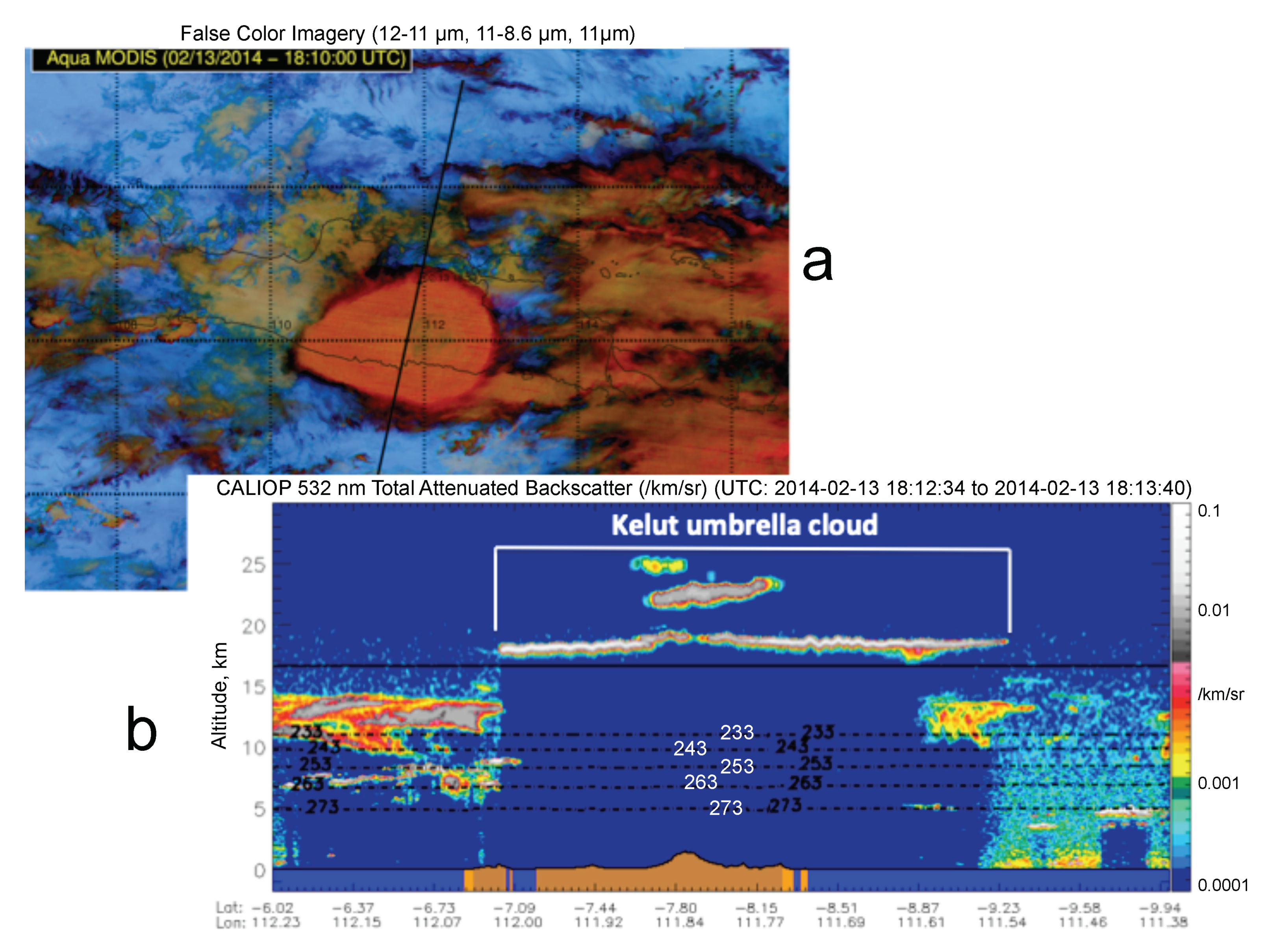
| Kelut | 13 February 2014, 1632 UT | 15.3 | 2.8 | 1 |
| Manam | 27 January 2005, 1400 UT | 24.0 | 3.0 | 1 |
| Manam | 24 October 2004, 2325 UT | 18.5 | 1.5 | 1 |
| Pinatubo | 15 June 1991, 2241 UT | 23.6 | 4.7 | 1 |
| Redoubt | 21 April 1990, 1412 UT | 12.0 | 4.9 | 2 |
| Mount St. Helens | 18 May 1980, 2020 UT | 13.0 | 1.0 | 1 |
| Date | Cloud | Height Range, km ASL | Depth, km | Age, hr | No. Layers |
|---|---|---|---|---|---|
| 15 April | 20100415 | 1.41–3.23 | 0.51 | <6 | – |
| 16 April | 20100416-a | 3.77–5.50 | 0.58 | 30 | >1 |
| 16 April | 20100416-b | 1.97–7.27 | 0.67 | 24 | >1 |
| 17 April | 20100417-a | 0.20–6.28 | 0.76 | 42 | 1 |
| 17 April | 20100417-b | 0.05–4.00 | 0.61 | 42 | 1 |
| 18 April | 20100418-a | 3.14–5.59 | 0.81 | 66 | – |
| 18 April | 20100418-b | 3.75–6.49 | 0.86 | 66 | – |
| 19 April | 20100419-a | 3.20–5.26 | 1.06 | 71 | – |
| 19 April | 20100419-c | 2.48–3.94 | 0.45 | 30 | – |
| 19 April | 20100419-d | 4.63–5.20 | 0.41 | 114–126 | – |
| 20 April | 20100420 | 0.05–1.88 | 1.08 | 20–24 | – |
| 4 May | 20100504 | 2.3–5.5 | 0.5 | – | 1–2 |
| 5 May | 20100505 | 2.4–4.5 | 0.9 | – | 1–2 |
| 14 May | 20100514 | 5.1–8.1 | 1.1 | – | 1–3 |
| 16 May | 20100516 | 3.4–5.5 | 1.2 | – | 1–3 |
| 17 May | 20100517 | 3.5–5.6 | 1.3 | – | 1–3 |
| 18 May | 20100518 | 2.5–4.9 | 0.9 | – | 1–3 |
| 19 April | 20100419-1 | 3.9-5.6 | 1.7 | 105–111 | >1 |
| 19 April | 20100419-2 | 3.5–3.8 | 0.3 | 104–108 | 1 |
| 19 April | 20100419-3 | 3.9–4.2 | 0.3 | 105–108 | 1 |
| 22 April | 20100422-4 | 0.7–5.5 | – | 49–50 | diffuse |
| 23 April | 20100423-5 | 2.1–3.4 | 1.3 | 40–58 | >1 |
| 2 May | 20100502-6 | 1.6–3.7 | 2.1 | 7.1–12 | >1 |
| 9 May | 20100509-7 | 3.5–4.9 | 1.4 | 97–129 | 1 |
| 13 May | 20100513-8 | 2.8–5.4 | 0.4–0.7 | 71–78 | 1 tilted |
| 16 May | 20100516-9 | 3.6–7.0 | 3.4 | 58–66 | >1 |
| 17 May | 20100517-10 | 3.2–6.3 | 3.1 | 66–88 | >1 |
| 18 May | 20100518-11 | 2.8–3.4 | 0.6 | 81–100 | 1 |
| 18 May | 20100518-12 | 4.0–5.7 | 1.7 | 66–78 | >1 |
| Diameter | Settling Speed † | ||||
|---|---|---|---|---|---|
| m | , m/s | m/s | m/s | m/s | m/s |
| 4000 | 5 | 16 | 1 | 51,020 | 0.86 |
| 1000 | 3 | 9.7 | 0.61 | 30,612 | 0.52 |
| 250 | 0.5 | 1.6 | 0.1 | 5102 | 0.086 |
| 100 | 0.1 | 0.32 | 0.02 | 1020 | 0.017 |
| 30 | 0.01 | 0.032 | 0.002 | 102 | 0.0017 |
| 10 | 0.0026 | 8.2 | |||
| 1 | 0.1 |
| Parameter↓|Model→ | Test, Nonlayered | Test, Layered | Pinatubo |
|---|---|---|---|
| Simulation type | VATD | Lagrangian | Lagrangian and VATD |
| Source type | Point | Point | Distributed |
| Source height, km | 4.2 | 4.2 to 10 | 23–27 |
| Particle size tested, m | 10–100 | 1–4000 | 1–1000 |
| Settling speed tested, m/s | –0.1 | –1.1 | –1.1 |
| Amount | 10 km | 1000 parcels | 1000 parcels |
| Duration of release | 0.02 h | Instantaneous | Instantaneous |
| Turbulent layer heights, km | – | 2.1–2.7, 3.8–4.2 | 24–25, 14.5–19 |
| Turbulent diffusivity, m/s | 500 | 0.098, 5800 | 0.098, 5800 |
Publisher’s Note: MDPI stays neutral with regard to jurisdictional claims in published maps and institutional affiliations. |
© 2021 by the authors. Licensee MDPI, Basel, Switzerland. This article is an open access article distributed under the terms and conditions of the Creative Commons Attribution (CC BY) license (http://creativecommons.org/licenses/by/4.0/).
Share and Cite
Bursik, M.; Yang, Q.; Bear-Crozier, A.; Pavolonis, M.; Tupper, A. The Development of Volcanic Ash Cloud Layers over Hours to Days Due to Atmospheric Turbulence Layering. Atmosphere 2021, 12, 285. https://doi.org/10.3390/atmos12020285
Bursik M, Yang Q, Bear-Crozier A, Pavolonis M, Tupper A. The Development of Volcanic Ash Cloud Layers over Hours to Days Due to Atmospheric Turbulence Layering. Atmosphere. 2021; 12(2):285. https://doi.org/10.3390/atmos12020285
Chicago/Turabian StyleBursik, Marcus, Qingyuan Yang, Adele Bear-Crozier, Michael Pavolonis, and Andrew Tupper. 2021. "The Development of Volcanic Ash Cloud Layers over Hours to Days Due to Atmospheric Turbulence Layering" Atmosphere 12, no. 2: 285. https://doi.org/10.3390/atmos12020285