Sensitivity of an Idealized Tropical Cyclone to the Configuration of the Global Forecast System–Eddy Diffusivity Mass Flux Planetary Boundary Layer Scheme

Abstract

The intensity and structure of simulated tropical cyclones (TCs) are known to be sensitive to the planetary boundary layer (PBL) parameterization in numerical weather prediction models. In this paper, we use an idealized version of the Hurricane Weather Research and Forecast system (HWRF) with constant sea-surface temperature (SST) to examine how the configuration of the PBL scheme used in the operational HWRF affects TC intensity change (including rapid intensification) and structure. The configuration changes explored in this study include disabling non-local vertical mixing, changing the coefficients in the stability functions for momentum and heat, and directly modifying the Prandtl number (Pr), which controls the ratio of momentum to heat and moisture exchange in the PBL. Relative to the control simulation, disabling non-local mixing produced a ~15% larger storm that intensified more gradually, while changing the coefficient values used in the stability functions had little effect. Varying Pr within the PBL had the greatest impact, with the largest Pr (~1.6 versus ~0.8) associated with more rapid intensification (~38 versus 29 m s⁻¹ per day) but a 5–10 m s⁻¹ weaker intensity after the initial period of strengthening. This seemingly paradoxical result is likely due to a decrease in the radius of maximum wind (~15 versus 20 km), but smaller enthalpy fluxes, in simulated storms with larger Pr. These results underscore the importance of measuring the vertical eddy diffusivities of momentum, heat, and moisture under high-wind, open-ocean conditions to reduce uncertainty in Pr in the TC PBL.

1. Introduction

The parameterization of the planetary boundary layer (PBL) in numerical weather prediction models determines how the momentum and enthalpy fluxes from the surface affect the lower atmosphere [1]. It is known that these fluxes play a key role in modulating tropical cyclone (TC) intensity and structure [2,3,4,5], which makes the PBL parameterization critical for achieving accurate TC forecasts. The operational Hurricane Weather Research and Forecast system (HWRF) [6,7,8,9] is NOAA’s flagship regional TC prediction system. The atmospheric model includes a variant of the same PBL parameterization—the Global Forecast System–Eddy Diffusivity Mass Flux (GFS-EDMF) scheme—which has been used in the operational Global Forecast System (GFS) since 2015. Readers should note that a newer PBL scheme that predicts turbulent kinetic energy [10] is planned for use in the operational GFS beginning in 2021. However, at the time of publication there were no plans to use this scheme in the operational HWRF. Therefore, it will not be discussed further here.

The local vertical mixing in the GFS-EDMF PBL is given by a K-profile parameterization, in which the boundary layer height (h) is diagnosed and the eddy diffusivity (K) is specified by a polynomial, subject to the conditions that $K=\kappa \left(\frac{u^{*}}{\mathsf{\phi }}\right)z$ in the surface layer and K = 0 at z = h [11]:

$$K=\kappa \left(\frac{u^{*}}{\mathsf{\phi }}\right)z{\left(1-\frac{z}{h}\right)}^p$$

(1)

where $\kappa =0.4$ is the von Karman constant, u^* is the friction velocity, φ is a stability function, and p is a shape parameter typically set to two. Depending on the stability, momentum does not necessarily diffuse at the same rate as heat or moisture, although the ratio of the vertical eddy diffusivity of momentum (K_m) to that of heat (K_h) is often assumed to be close to one, especially in the near-neutral conditions that characterize the TC PBL [12,13]. This ratio is known as the turbulent Prandtl number (Pr).

Some previous research examined the utility of different PBL scheme classes for TC prediction [11,13,14,15]. These studies found that PBL schemes containing K-profile parameterizations with p = 2, like the GFS-EDMF, are overly diffusive in the TC PBL. Extensive work has been undertaken to ameliorate this problem in HWRF. Consistent with these previous studies, low-altitude aircraft observations of K_m in the open-ocean TC PBL [16] revealed that the K_m values in earlier versions of HWRF were too large in hurricane conditions over the water [17]. When the magnitude of K_m was reduced to be more consistent with the observations using a tuning parameter (α; discussed in more detail in Section 2), the TC intensification rate and peak intensity increased due to shallower but stronger boundary-layer inflow [18,19,20,21]. When it was implemented in the 2012 operational HWRF, the reduction in K_m contributed to substantial increases in the forecast skill for TC track (+9%), intensity (+30%), and tropical storm-force wind radius (+80%) in the eastern North Pacific basin, with smaller but still significant improvements in the North Atlantic [22]. Initially, K_m was uniformly decreased in the PBL by 50% (2012 HWRF) or 30% (2013–2014 HWRF) [23]. However, more sophisticated techniques soon evolved that varied the K_m reduction with wind speed and height above the surface [8,24], which remain in place as of the 2020 HWRF.

In addition to the K_m modifications, previous work also improved the representation of the TC PBL height in HWRF. In the GFS-EDMF, the PBL height is proportional to the critical bulk Richardson number (Ric). Early versions of the scheme in HWRF used Ric = 0.5. Previous research suggests that PBL schemes that use a fixed value of Ric to determine PBL height tend to overestimate it, especially in hurricanes [14,17]. As a result, Ric was first reduced to 0.25 (HWRF 2012) and then made to vary with the surface Rossby number (HWRF 2013–onward) [23], based on the results of [25]. The result is that the TC PBL height in HWRF became smaller as the model matured, acting to reduce K_m further.

The aforementioned changes have led to substantial improvements in the forecast skill of the operational HWRF and are generally regarded as major accomplishments of the National Oceanic and Atmospheric Administration’s Hurricane Forecast Improvement Program [26]. However, room for improvement remains. Compared to observations, the HWRF PBL is overly unstable, and the upper portion of the PBL is too cool and dry [23]. In addition, rapid intensification remains a difficult forecast challenge.

Most previous studies of TCs and the GFS-EDMF PBL or its predecessors focused on either the K_m parameterization [17,18,19,20,21,22] or on comparing its performance with that of other PBL schemes [14,15,27,28]. In this paper, we instead analyze the relative roles of several other parts of the GFS-EDMF scheme in controlling TC evolution, intensity, and structure, including the non-local portion of the GFS-EDMF, the stability functions for heat and momentum, and Pr. The motivation for documenting TC sensitivity to these other elements of the GFS-EDMF is to offer potential new ways to modify the scheme for operational TC prediction.

The next section provides an overview of the GFS-EDMF PBL. Section 3 describes the model setup and the experiments. Results are presented in Section 4, along with a discussion of how the results from the different experiments relate. A summary of the paper and its conclusions appears in Section 5.

2. Background

The GFS-EDMF PBL consists of both local and non-local vertical mixing parameterizations. The overall diffusive tendency of a prognostic variable X (e.g., zonal and meridional wind speed, potential temperature, or water vapor mixing ratio) [8] is given by

$$\frac{\partial X}{\partial t}=\frac{\partial }{\partial z}\left[K_X\left(\frac{\partial X}{\partial z}\right)-F_{X,NL}\right]$$

(2)

The first term in brackets in the above equation represents the contribution from the local vertical mixing scheme to the vertical diffusion of X. The local scheme uses K-theory to relate the time tendencies of the prognostic variables to the eddy diffusivity (K_X) and vertical gradient of X. The local scheme is described in more detail below and in previous studies [29,30]. The form of the non-local term F_X,NL varies depending on the stability [31]. In weakly unstable conditions, a countergradient term is used to represent the non-local fluxes of heat and momentum [29,30,31]:

$$F_{X,NL}=c\frac{{\left(\overline{w^{\prime }{X}^{\prime }}\right)}_0}{w_{s}h}$$

(3)

where c is a coefficient of proportionality assumed to be equal to 6.5 in the GFS-EDMF PBL [29], ${(\overline{w^{\prime }{X}^{\prime }})}_0$ is the surface flux of X, w_s is a velocity scale, and h is the PBL height. Under strongly unstable conditions, the GFS-EDMF PBL uses a mass-flux scheme to determine the non-local fluxes [8,31]:

$$F_{X,NL}=M\left(X_u-\overline{X}\right),$$

(4)

where M is the updraft mass flux, X_u is the value of X in the updraft, and $\overline{X}$ is the value of X in the environment. While local mixing is always active, a dimensionless stability parameter (𝛇 = z₁/L), where z₁ is the height of the first model vertical level and L is the Obukhov length, is used to determine whether to activate the non-local mixing components, according to the criteria in

Table 1. Relationship between 𝛇 and Global Forecast System–Eddy Diffusivity Mass Flux (GFS-EDMF) planetary boundary layer (PBL) scheme behavior.

Range of 𝛇	Active Components
𝛇 > 0.2	Local mixing
−0.5 ≤ 𝛇 ≤ 0.2	Local mixing; countergradient mixing
𝛇 < −0.5	Local mixing; mass-flux mixing

.

$$F_{X,NL}=c\frac{{\left(\overline{w^{\prime }{X}^{\prime }}\right)}_0}{w_{s}h}$$

(5)

A few other details about the local vertical mixing scheme are relevant to this study. The K_m parameterization has received a lot of attention in HWRF and is worth discussing in more depth. K_m is calculated from a cubic function that depends on the height above the surface (z), h, the stability function for momentum (φ_m), the surface friction velocity (u*), and the tuning parameter (α) discussed in Section 1:

$$K_m=\kappa \left(\frac{u^{*}}{{\phi }_m}\right)z\left[\alpha {\left(1-\frac{z}{h}\right)}^2\right]$$

(6)

K_h and the vertical eddy diffusivity of the water vapor mixing ratio (K_q) are assumed to be equal and are obtained by multiplying K_m by the inverse of Pr:

$$K_h=K_q=\frac{K_m}{Pr}$$

(7)

K_h and K_q are ultimately used to calculate the enthalpy fluxes [12]:

$$SHF=-\rho c_p{K}_h\frac{d\theta }{dz}$$

(8)

$$LHF=-\rho L_v{K}_q\frac{dq}{dz}$$

(9)

where SHF is the sensible heat flux, ρ is the air density, c_p is the specific heat of air at constant pressure, dθ/dz is the vertical gradient of potential temperature, LHF is the latent heat flux, L_v is the latent heat of vaporization, and dq/dz is the vertical gradient of the water vapor mixing ratio.

Because Pr is used to determine K_h and K_q, which in turn are needed to calculate the enthalpy fluxes that sustain the TC, Pr is an important parameter in the GFS-EDMF. When the non-local countergradient (but not the mass-flux) mixing scheme is active, Pr is calculated according to the following equation:

$$Pr=\frac{{\phi }_h}{{\phi }_m}+c\kappa z_s$$

(10)

where z_s is the assumed fractional depth of the surface layer relative to the entire depth of the PBL. Since z_s = 0.1 and c = 6.5 in the version of the GFS-EDMF PBL used in HWRF, the entire second term is a constant equal to 0.26. When there is either only local mixing (𝛇 > 0.2) or the non-local mass-flux scheme is activated (𝛇 < −0.5), Pr is simply the ratio of the stability function for heat to the stability function for momentum. The stability functions are taken from Dyer and Hicks [32]:

$${\phi }_m={(1-16\frac{z_{s}h}{L})}^{-0.25}, R_i\le 0$$

(11)

$${\phi }_h={(1-16\frac{z_{s}h}{L})}^{-0.5}, R_i\le 0$$

(12)

$${\phi }_m=1+5\frac{z_{s}h}{L}, R_i>0$$

(13)

$${\phi }_h=1+5\frac{z_{s}h}{L}, R_i>0$$

(14)

where R_i is the bulk Richardson number. The first set of stability functions is applied in the unstable regime (R_i ≤ 0), while the second set is applied in the stable regime (R_i > 0). While Dyer and Hicks [32] use the classical definition of 𝛇 = z/L, the GFS-EDMF PBL uses a different quantity ($z_{s}h/L$) in place of 𝛇 to calculate the stability functions. The implications of this choice are discussed in Section 4.2.

3. Methods

The idealized configuration of HWRFv3.9a [8] was used in this study. This version of the model is consistent with the 2017 operational HWRF, but the idealized configuration does not include ocean or wave coupling, vortex initialization, or data assimilation. Instead, the model is initialized with a quiescent sounding that is based on the mean vertical profiles of temperature and humidity from June to September in the Caribbean as reported by Jordan [33]. An idealized vortex, with an initial horizontal wind speed (i.e., intensity) of 20 m s⁻¹ and a radius of maximum wind (RMW) of 90 km, is then superimposed on the base state. The idealized vortex is described in more detail in [34]. There is no land in the model domain, and the sea-surface temperature (SST) is held constant at 302 K (28.85 °C). In all other respects, the idealized HWRFv3.9a configuration and the 2017 operational HWRF are equivalent, and utilize the same 18–6–2 km triply-nested configuration and the same atmospheric physics, which are listed in

Table 2. The physics schemes used in the idealized Hurricane Weather Research and Forecast system (HWRF).

Type	Description
Shortwave, longwave radiation	Rapid Radiative Transfer Model for general circulation models (RRTMG)
Cumulus	scale-aware Simplified Arakawa-Schubert (scale-aware SAS)
Microphysics	modified tropical Ferrier-Aligo
Planetary boundary layer	GFS-EDMF
Surface layer	Geophysical Fluid Dynamics Laboratory (GFDL)
Land surface	None

and discussed in more detail in [8]. While the operational HWRF has been upgraded multiple times since 2017, there have not been any changes to the PBL scheme, and most of the remaining changes are related to improving the initialization system (i.e., vortex initialization and data assimilation), which is not utilized here. The simplified initial conditions and the lack of ocean coupling make it easier to isolate the impact of PBL scheme changes on the TC, due to the reduced number of nonlinear interactions relative to the operational system.

The first simulation that was conducted utilizes the default configuration of the HWRF PBL that is contained in HWRFv3.9a and is described in the previous section. This control simulation will be referred to as CTRL hereafter. Three modifications to the PBL scheme are then tested in individual experiments. The first change (LOCAL-MIXING) studies the impact of disabling the non-local vertical mixing (i.e., the countergradient and mass-flux components of the vertical mixing) on the TC intensity and structure. The purpose of this experiment is to understand the relative roles of the local and non-local vertical mixing in the TC PBL. We note that some sources of non-local vertical mixing, such as mixing caused by partially-resolved individual updrafts and downdrafts associated with convection, will still be present in the LOCAL-MIXING simulation. Therefore, this experiment only investigates the TC sensitivity to the subgrid-scale (SGS) non-local vertical mixing in the PBL. Relative to CTRL, disabling this SGS non-local vertical mixing in the PBL leads to a smaller Pr, since the second term in Equation (9) is eliminated when countergradient fluxes are not active. Equation (6) suggests that smaller Pr increases K_h, which enhances the enthalpy flux from the ocean to the atmosphere for a given near-surface wind speed (Equations (7)–(8)). Therefore, it is reasonable to expect that changes to the HWRF PBL that impact K_h might affect the TC intensity and structure.

The second change (BUSINGER-PHI) replaces the stability functions for momentum and heat from Dyer and Hicks [32] (Equations (10)–(13)), with an alternative form proposed by Businger et al. [35] (Equations (14)–(17)):

$${\phi }_m={(1-15\frac{z_{s}h}{L})}^{-0.25}, R_i\le 0$$

(15)

$${\phi }_h=0.74{(1-9\frac{z_{s}h}{L})}^{-0.5}, R_i\le 0$$

(16)

$${\phi }_m=1+4.7\frac{z_{s}h}{L}, R_i>0$$

(17)

$${\phi }_h=0.74+4.7\frac{z_{s}h}{L}, R_i>0$$

(18)

φ_m and φ_h are used to calculate K_m, K_h, and Pr via Equations (5), (6) and (9), respectively. The effect of this change is to decrease Pr slightly, but to a much lesser extent than in LOCAL-MIXING, which we will show later. In a final experiment (Pr = 1.58), the Pr within the PBL is set to a constant value of 1.58, which is much larger than that suggested by either the Dyer or Businger relations, to bookend the results from the other simulations. This specific Pr value was chosen because observations of K_m and K_h in the TC PBL collected during the Coupled Boundary Layer Air–Sea Transfer (CBLAST) experiment imply a mean Pr of 1.58 [12]. Above the PBL, the formulation for Pr was not changed. Because there is substantial scatter in the individual values of Pr = K_m/K_h from CBLAST, this experiment is undertaken as a sensitivity test, and is not meant to imply that a Pr of 1.58 is a reasonable choice throughout the TC PBL. This point is discussed in more detail in Section 4.4.

While the above experiments may appear to be unrelated, we will show later that each of their results can be explained by understanding their impact on Pr and K_h.

Table 3. The experiments conducted in this study.

Experiment	Description
CTRL	Default HWRF PBL configuration
LOCAL-MIXING	Non-local vertical mixing disabled
BUSINGER-PHI	Replace Dyer’s φm and φh with Businger’s
Pr = 1.58	Set Pr to 1.58 in the PBL

summarizes the control and experiment simulations.

In each experiment, the GFDL vortex tracker [36] was used in the inner nest (vortex_tracker option 7 in the namelist) to track the storm center position, maximum 10-m wind speed, and minimum sea-level pressure. The parameters used to estimate the storm center location were the (1) relative vorticity at 10 m, 850 hPa, and 700 hPa; (2) horizontal wind speed at 10 m, 850 hPa, and 700 hPa; (3) mean sea-level pressure; and (4) geopotential height at 850 hPa and 700 hPa. The version of the tracker used here ran concurrently with the HWRF forecast, providing updated storm information every 6 min. The inline tracker is identical to the external tracker that runs as a postprocessing step in the operational HWRF, with the exception that the internal tracker does not attempt to detect TC dissipation. Since dissipation does not occur in any of our simulations, we expect our results to be comparable to those produced by the external tracker.

While the GFDL vortex tracker is capable of providing wind radii information, we chose to calculate our own radii of 34-kt (tropical-storm force), 64-kt (hurricane-force), and maximum winds (1 kt = 0.514 m s⁻¹). For this purpose, we transformed the three-dimensional model output from the inner nest to cylindrical coordinates (relative to the TC center) and calculated the wind radii as a function of height from the azimuthally-averaged wind field. The GFDL vortex tracker, in contrast, only provides the wind radii at 10 m. In addition, the tracker calculates the maximum extent of each wind radius, rather than the values from the azimuthally-averaged wind field that we computed. Considering the wind radii of the azimuthally-averaged wind field reduces noise in the time series, making it easier to visualize differences in the storm size between the various experiments.

4. Results and Discussion

4.1. Characteristics of the CTRL Simulation

Shortly after initialization, the TC in CTRL has an intensity of ~15 m s⁻¹ (Figure 1a) and a RMW of 90 km (Figure 1c). During the first day of the simulation, a period of rapid intensification [37] ensues, with the RMW contracting to ~20 km and the storm intensity increasing to ~53 m s⁻¹ by t = 24 h. A brief period of weakening occurs from t = 40–60 h before the storm reaches a second, stronger peak intensity of ~70 m s⁻¹ around t = 100 h. Some fluctuations in intensity occur during the final day of the simulation (t = 100–120 h). There is generally close correspondence between the trends in maximum wind speed and minimum central pressure (Figure 1b). The storm size increases as the TC matures, with the radius of 34-kt winds (dotted black line in Figure 1c) approximately doubling from t = 20 to 120 h.

Because the value of 𝛇 = z₁/L determines whether and what kind of non-local mixing is active within a particular vertical column of the model simulation (Table 1), it is useful to examine the spatial distribution of z₁/L within the TC to understand the behavior of the GFS-EDMF scheme there. Figure 2 shows the value of z₁/L on the innermost HWRF domain for three different forecast hours in CTRL during the mature stage of the TC. The 34-, 50-, and 64-kt wind contours (black lines in Figure 2) are also shown to demonstrate how the model values of z₁/L correspond to the TC structure. In general, stability increases with decreasing distance from the TC center, which is consistent with the assumption that the TC PBL is near neutral (z₁/L~0). The value of z₁/L is less than 0.2 everywhere in the domain, indicating that countergradient fluxes are active both inside the TC and within the environment (Table 1). However, there are only small, isolated areas where z₁/L is less than −0.5 and the mass flux scheme is active (white areas in Figure 2). The regions that have z₁/L near or less than −0.5 are all associated with rainbands. This result suggests that the mass flux scheme probably does not play a substantial role in modulating TC structure or intensity.

The maintenance of positive temperature and moisture contrasts between the ocean and the atmosphere (sea minus air) is essential for sustaining the enthalpy fluxes that drive the TC heat engine. Here, we examine the difference in the air temperature (dT; Figure 3a) and water vapor mixing ratios (dq; Figure 4a) between the ocean surface and the first model vertical level (approximately 10-m height), since those are the quantities and vertical levels that the GFDL surface layer scheme uses to calculate the fluxes from the ocean to the atmosphere. To calculate the water vapor mixing ratio at the ocean surface, we assume that the SST is equal to the air temperature and that the air is saturated (i.e., 100% relative humidity). Within the 50-kt wind radius, dT and dq range from 3 to 4 K (Figure 3a) and 6–7.5 g kg⁻¹ (Figure 4a), respectively, at t = 120 h in CTRL. The model values are about 50% larger than buoy observations of dT and dq at 10-m height in hurricanes [38], which is consistent with the overly-unstable HWRF PBL noted in previous studies [23,39]. The shape of the observed and simulated radial distributions of dT and dq, however, are qualitatively similar. These values of dT and dq contribute to total (sensible + latent) enthalpy fluxes of up to 1850 W m⁻² within the 50-kt wind radius (Figure 5a), which we refer to as the TC inner core in the remainder of this study.

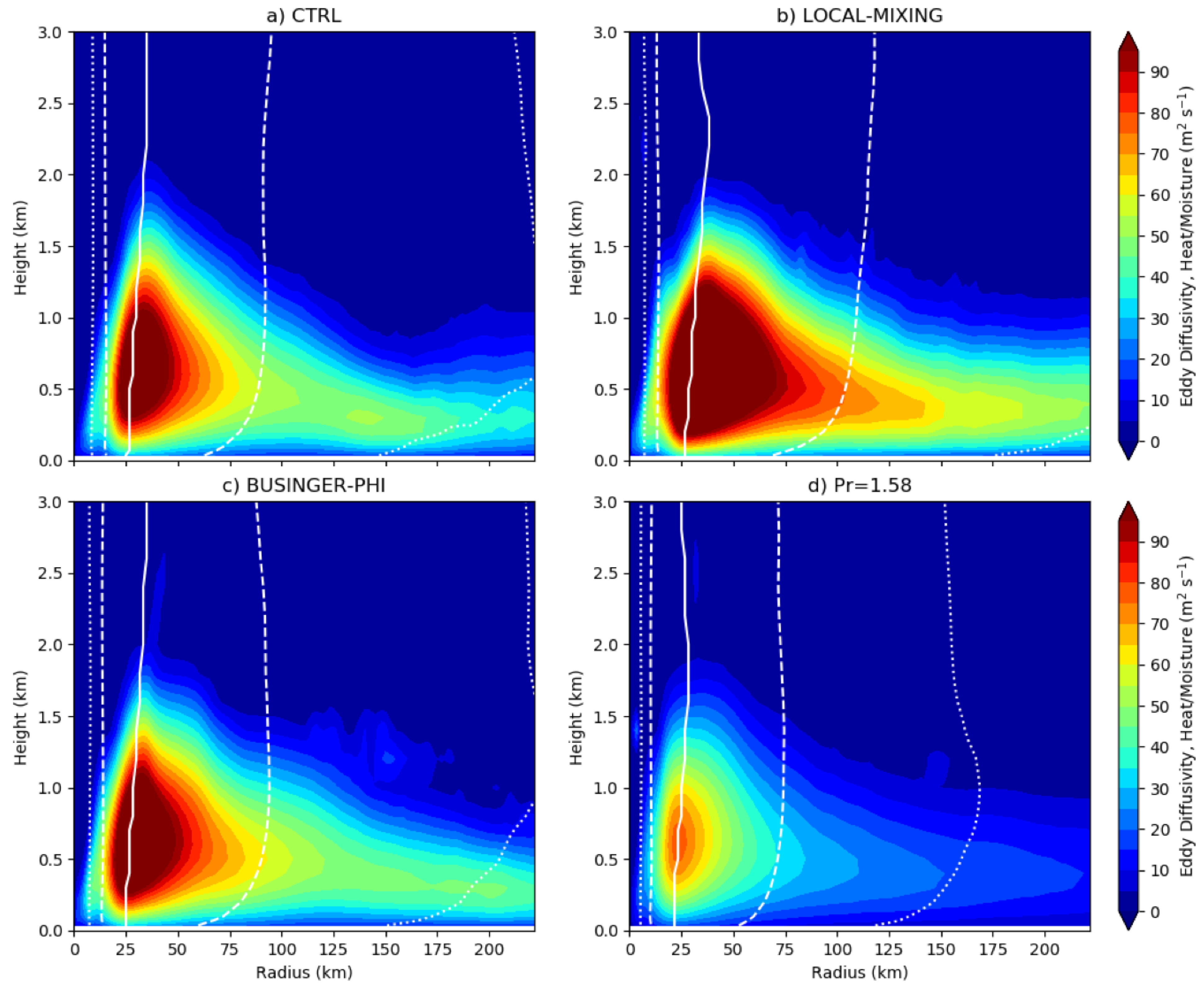
4.2. Non-local Mixing and Simulated Tropical Cyclones

To determine whether TCs are sensitive to non-local mixing in the GFS-EDMF PBL, we performed an experiment (LOCAL-MIXING) in which the mass-flux scheme was deactivated and the countergradient term was set to zero throughout the model domain. This leaves only the local mixing scheme active. Figure 1a demonstrates that when non-local mixing is disabled, the TC intensifies more gradually, reaching a weaker initial peak intensity (58 m s⁻¹) than in CTRL (63 m s⁻¹). However, the storm in LOCAL-MIXING eventually obtains the same peak wind speed as the CTRL storm, and maintains this wind speed, along with a smaller minimum central pressure (Figure 1b), for a longer portion of the t = 100–120 h period. An additional difference between the CTRL and LOCAL-MIXING storms is that the various wind radii are larger in LOCAL-MIXING, with a ~15% larger 34-kt wind radius (Figure 1c).

Relative to the CTRL storm, the total enthalpy flux in the LOCAL-MIXING storm is 15–50% larger within the 50-kt wind radius at t = 120 h (Figure 5b). At t = 120 h, the CTRL and LOCAL-MIXING storms have the same intensity (Figure 1a), which indicates that the difference in the enthalpy fluxes is mainly driven by differences in dT and dq rather than wind speed. Indeed, dT (Figure 3b) and dq (Figure 4b) are roughly 15–40% larger within the 50-kt wind radius in the LOCAL-MIXING simulation. The larger sea–air contrasts and greater enthalpy fluxes in LOCAL-MIXING are explained by the reduction in Pr that occurs in this experiment (Figure 6b) relative to CTRL (Figure 6a). The smaller Pr in LOCAL-MIXING is due to disabling the countergradient fluxes, which eliminates the second term in the Pr calculation (Equation (9)) and reduces Pr by 0.26 when −0.5 ≤ 𝛇 ≤ 0.2. The smaller Pr leads to increased K_h (Equation (6)), K_q (Equation (6)), and enthalpy fluxes in the PBL (Equations (7)–(8)). Recall that the dimensionless ratio used to calculate the stability functions in the GFS-EDMF is $z_{s}h/L$, not 𝛇. The effect of this choice is to reduce Pr below the value implied by the Dyer relation (black line in Figure 6b) for a given value of 𝛇. In CTRL, the addition of the second term in Equation (9) boosts Pr close to the values suggested by the Dyer relation, but only when countergradient fluxes are active (Figure 6a). The relationship between Pr, K_h, and the enthalpy fluxes will be discussed in greater detail in Section 4.4.

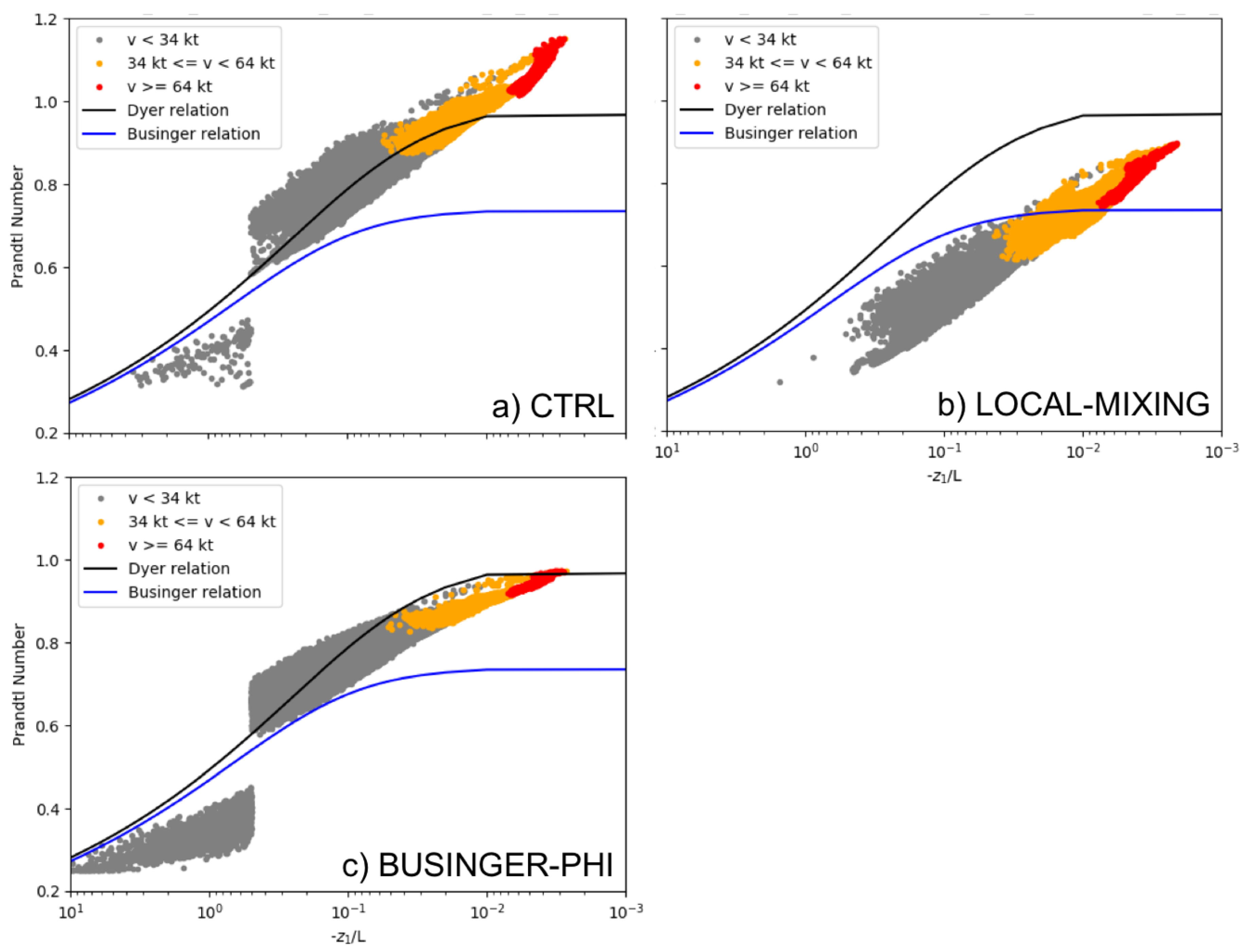
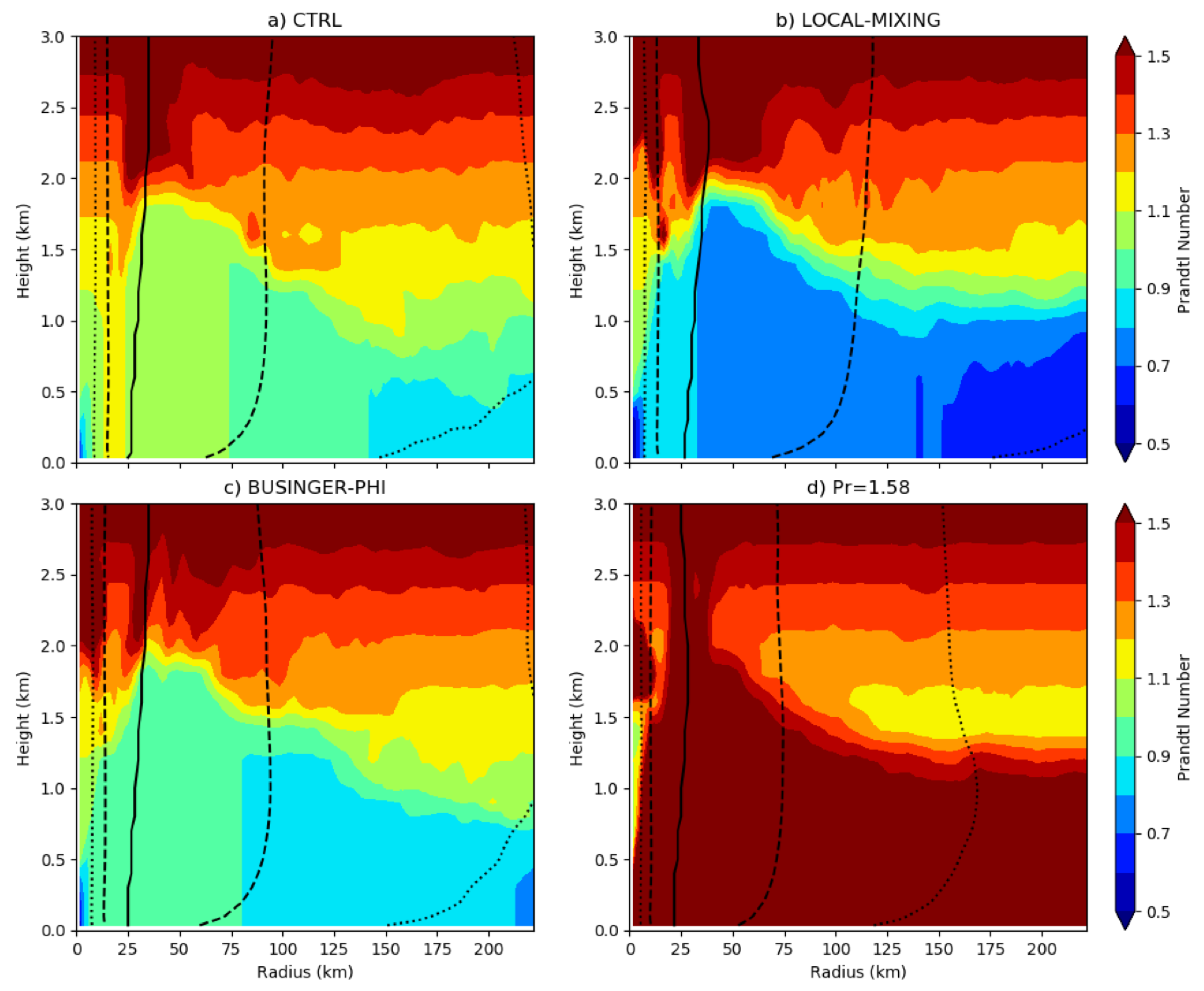
4.3. Stability Functions and Simulated Tropical Cyclones

Within the GFS-EDMF PBL, the stability functions for heat and momentum are taken from Dyer (Section 2; Equations. (10)–(13)). These stability functions are used within the PBL to calculate Pr from Equation (9). In a third experiment (BUSINGER-PHI), Dyer’s coefficients were replaced with Businger’s (Equations (14)–(17)) in the GFS-EDMF PBL to determine whether this particular choice of stability functions impacts TC intensity and structure. BUSINGER-PHI produces a storm that has a slightly weaker peak intensity, with a maximum wind that is ~5 m s⁻¹ weaker than CTRL for most forecast lead times from 80 to 120 hours (Figure 1a). The minimum central pressure is also about 5 hPa larger during most of the simulation after the first 36 h (Figure 1b). In general, the storm created in BUSINGER-PHI also does not intensify as rapidly as the storm in CTRL and takes almost twice as long to exceed an intensity of 60 m s⁻¹. The CTRL and BUSINGER-PHI storms have fairly similar wind radii (Figure 1c). Overall, dT (Figure 3c), dq (Figure 4c), and the total enthalpy flux (Figure 5c) do not show a consistent change relative to CTRL in the TC inner core. Unlike in the LOCAL-MIXING experiment, Pr is only slightly smaller in the BUSINGER-PHI experiment than in CTRL (by about 0.1; Figure 6c), which contributes to the similar sea–air contrasts and enthalpy fluxes in the latter two simulations. Figure 6c also indicates that the mass-flux scheme is more active in the TC environment in BUSINGER-PHI than in CTRL, since there are more points with weaker than tropical-storm-force winds that have 𝛇 < −0.5.

4.4. Tying the Results Together: Prandtl Number and Tropical Cyclones

The CBLAST experiment derived Pr from observations of K_m and K_h within the TC PBL in wind speeds that ranged from 18 to 30 m s⁻¹ [12]. Their observations suggest that Pr values below one, such as those in the LOCAL-MIXING experiment (Figure 6b), are too small for the hurricane environment. In fact, their K_m and K_h observations imply a mean Pr of 1.58 (Figure 9 in Zhang and Drennan [12]), which is much larger than the values in CTRL or in the experiments conducted so far. However, the applicability of these data to our model simulations is questionable, since the observations were made in multiple TCs at heights from 60 to 800 m in conditions that varied from weakly unstable to stable, as determined from the vertical gradient of potential temperature measured during the flights. In addition, there is substantial scatter in each individual value of Pr = K_m/K_h (their Figure 9), which suggests that the mean Pr value may not be particularly informative. For these reasons, we do not wish to imply that Pr = 1.58 is a realistic value to use throughout the TC PBL. Rather, our purpose is to determine the impact of using a larger Pr value on the structure and evolution of the TC. To consider this effect, a fourth experiment (Pr = 1.58) was conducted in which Pr was set to a fixed value of 1.58 within the PBL. Above the PBL, Pr was not changed.

The simulated maximum wind speed, minimum central pressure, and RMW from this experiment are shown by the green curves in Figure 1. Compared to the other three experiments, the TC in Pr = 1.58 undergoes the most rapid rate of deepening, reaching a sub-950-hPa pressure approximately ten hours earlier than the storms in the other experiments (Figure 1b). This rapid deepening is also reflected in the maximum wind. Notably, however, the minimum central pressure and maximum winds level off at values corresponding to a weaker storm than in the other experiments. In addition, the storm size, especially the 34-kt wind radius, is much smaller than in the control (100 km versus 125 km at t = 120 h).

How are the smaller storm size, greater propensity for rapid intensification, and weaker peak intensity in the Pr = 1.58 storm related? The comparison of the enthalpy fluxes in the four simulations suggests an explanation. The inner-core enthalpy fluxes at t = 120 h (Figure 5d) are up to 45% weaker in the Pr = 1.58 simulation than in CTRL. Even in the environment, the fluxes are notably weaker. While enthalpy fluxes are generally strongly correlated with wind speed, differences in wind speed do not explain why the enthalpy fluxes differ between these particular simulations, since at t = 120 h the storms have similar maximum wind speeds (Figure 1a). Instead, the air–sea temperature (Figure 3) and moisture contrasts (Figure 4) are substantially reduced in the Pr = 1.58 storm, which in turn reduces the enthalpy fluxes within both the environment and the TC inner core. In addition, because K_m is unchanged, the larger Pr (=K_m/K_h) implies smaller K_h for the same wind speed (Figure 7), which further reduces the enthalpy fluxes in the PBL via Equations (7)–(8). Regarding the smaller storm size in Pr = 1.58, controls on TC structure are not well understood, but a few studies have posited a relationship between storm size and the magnitude and aerial extent of the surface enthalpy fluxes [40,41]. If this relationship is valid, it may explain why the Pr = 1.58 storm is smaller than the storm in CTRL.

Regardless of the cause for the more compact TC in Pr = 1.58, smaller storms tend to intensify more rapidly [42,43,44,45], and the storm in Pr = 1.58 strengthens faster than the TCs in any of the other simulations (Figure 1). When the initial period of strengthening begins in Pr = 1.58 at around t = 10 h, the storm is weak with a peak wind of ~15 m s⁻¹, and it is presumed that large enthalpy fluxes are not needed to intensify such a weak TC. The RMW in Pr = 1.58, however, is already beginning to decrease below the RMW of the CTRL storm, and this trend continues throughout the RI period. Near the end of the RI period at t = 24 h, the maximum winds of the Pr = 1.58 storm have already exceeded 50 m s⁻¹. As the wind speed approaches the maximum intensity, the reduced enthalpy fluxes in the Pr = 1.58 storm play a larger role, and it reaches an earlier but weaker initial peak intensity (~57 m s⁻¹) than the storm in CTRL (63 m s⁻¹).

The Pr = 1.58 simulation is not the only experiment in which the relationship between Pr, enthalpy fluxes, storm size, intensification rate, and peak intensity is evident. Instead, the results from the LOCAL-MIXING experiment can also be explained through this mechanism. Figure 8 demonstrates that near the RMW within the PBL, the storm in the LOCAL-MIXING experiment has a Pr value of ~0.8, respectively, compared to 1.1 in CTRL (Figure 8). Within the TC inner core, LOCAL-MIXING also has larger sea–air contrasts (Figure 3 and Figure 4), K_h values at a given wind speed (Figure 7), and enthalpy fluxes (Figure 5) than CTRL, possibly leading to a larger storm size (Figure 1c). The LOCAL-MIXING TC intensifies more slowly than the CTRL and Pr = 1.58 storms during the first 36 h due to its larger size, but ultimately reaches a peak intensity that is comparable to or greater than the CTRL and Pr = 1.58 storms due to its larger enthalpy fluxes. In contrast, the changes to the stability functions in the BUSINGER-PHI experiment have a relatively minor impact on Pr (Figure 6c and Figure 8c), which explains why the CTRL and BUSINGER-PHI TCs are similar.

Although the impact of Pr on TC intensity change is evident, the most striking difference is the impact of Pr on the size of the tropical storm-force wind radius at 10-m height. At t = 120 h, the 34-kt wind radius is 100 km in the experiment with the largest Pr (Pr = 1.58), but 150 km in the experiment with the smallest Pr (0.8, LOCAL-MIXING), a remarkable 40% difference. Recent (2018–2020) versions of the operational HWRF exhibit a negative 34-kt wind radius bias, a near-neutral 50-kt wind radius bias, and positive 64-kt wind radius and RMW biases [46], so it is not clear that adjusting Pr in the operational system should be considered, since all of the wind radii will be affected. However, newer TC forecasting systems under development at the National Centers for Environmental Prediction that also use the GFS-EDMF PBL, such as the Hurricane Analysis and Forecast System, currently exhibit positive wind radii biases [47]. Adjustments to Pr in these models could be considered if they are done in a physically-consistent manner and do not degrade the TC track and intensity forecasts.

5. Summary and Conclusions

In this paper, we used an idealized version of HWRF to study the sensitivity of TC intensity and structure to several settings in the GFS-EDMF PBL, which is used in the operational HWRF. The model was initialized with an idealized vortex that was superimposed on a quiescent base state and ran for five days. The SST was fixed at 302 K (28.85 °C) throughout the simulation. The experiments included (1) disabling the non-local vertical mixing parameterizations in the PBL (LOCAL-MIXING), (2) replacing the coefficient values in the stability functions for momentum and heat with those proposed by Businger [35] (BUSINGER-PHI), and (3) using a larger value of the Prandtl number within the PBL (Pr = 1.58), consistent with TC PBL observations from the CBLAST experiment. The results from these experiments were compared to each other and to a control simulation (CTRL) with no changes.

The CTRL simulation produced a TC that underwent a period of rapid intensification (27 m s⁻¹ in 24 h) during the first day, peaking at 70 m s⁻¹ at t = 100 h before weakening slowly thereafter. The storm in the LOCAL-MIXING experiment intensified more slowly than the CTRL storm, but ultimately reached a similar peak intensity and maintained this intensity for a longer period of time. The modifications made in the LOCAL-MIXING experiment (i.e., disabling the non-local vertical mixing parameterizations in the GFS-EDMF) decreased Pr, which resulted in sea–air temperature and moisture contrasts that were 15–40% larger than in the CTRL storm and contributed to a 15–50% larger total enthalpy flux under similar wind conditions. The wind radii in the LOCAL-MIXING storm were ~15% larger than those in the CTRL simulation, possibly due to the larger enthalpy fluxes. Because the storm was larger, it intensified more slowly than the TC in CTRL.

In contrast, the larger Pr in the Pr = 1.58 storm reduced the temperature and moisture contrast between the ocean surface and the lowest model level (~10 m) by 30–40%, which decreased the enthalpy fluxes and resulted in a slightly weaker peak intensity (~65 m s⁻¹). All of the wind radii in the Pr = 1.58 storm were substantially smaller than those of the CTRL or LOCAL-MIXING storms, especially the 34-kt wind radius, which was 25% and 33% smaller than in the CTRL and LOCAL-MIXING storms, respectively. Despite the weaker peak intensity, the smaller size of the Pr = 1.58 storm allowed it to intensify even more rapidly in the first 24 h than the CTRL or LOCAL-MIXING storms. Unlike the LOCAL-MIXING or Pr = 1.58 experiments, modifying the stability functions in the BUSINGER-PHI experiment had a relatively small impact on Pr and the TC. The most notable difference in the BUSINGER-PHI experiment was that the storm was about 5 m s⁻¹ weaker than the CTRL storm, despite similar sea–air contrasts.

The above results suggest that the impact to Pr should be considered when future changes are made to the GFS-EDMF PBL. In the GFS-EDMF, when Pr is increased, the resulting TC:

• Has a smaller K_h and K_q for a given wind speed;
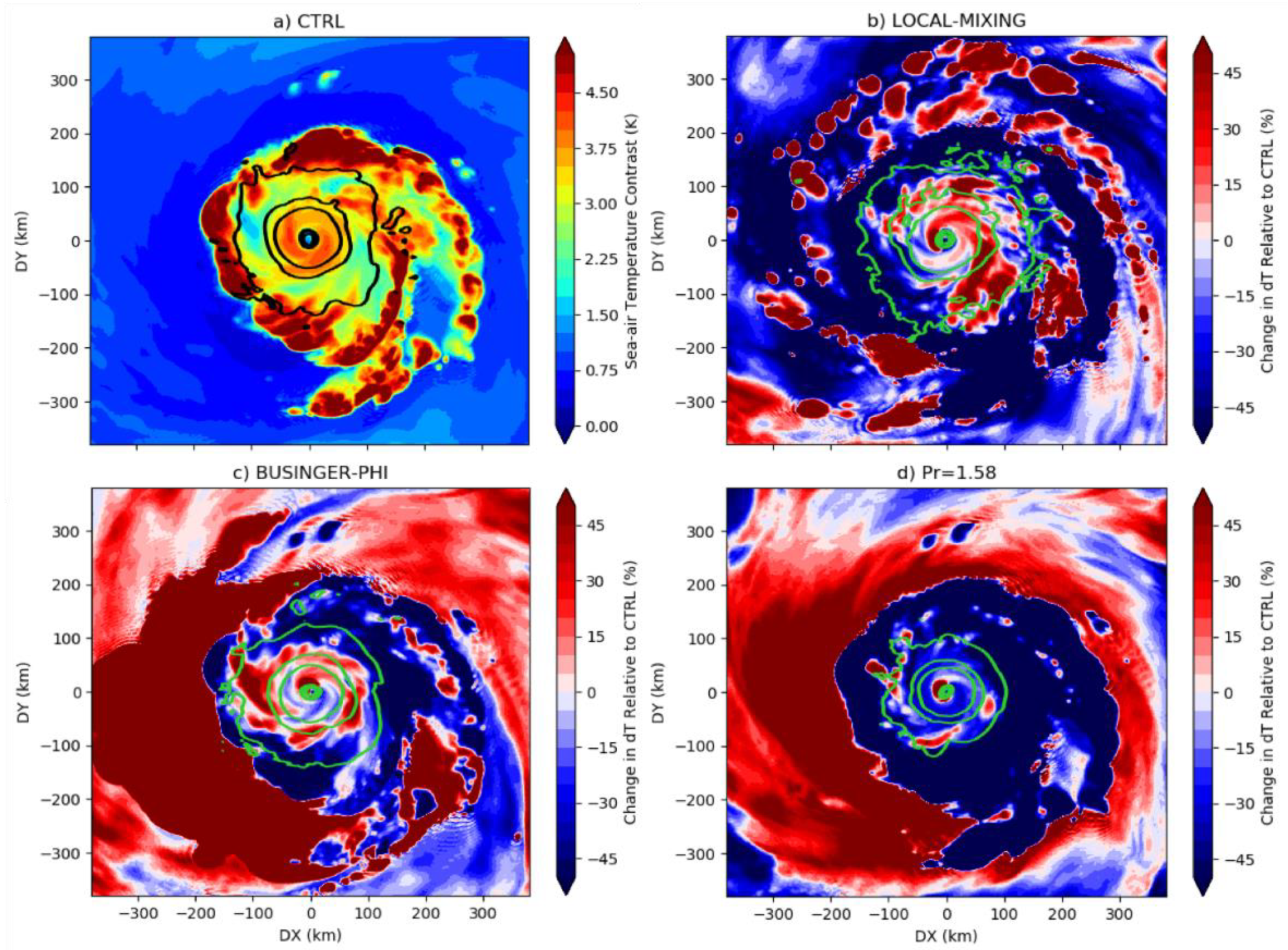
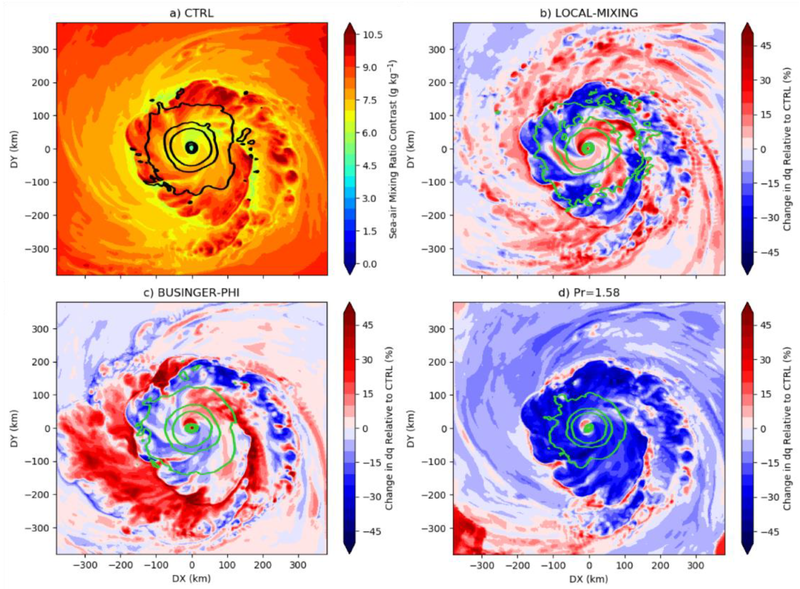
• Exhibits reduced enthalpy fluxes within its inner-core, even at similar wind speeds;
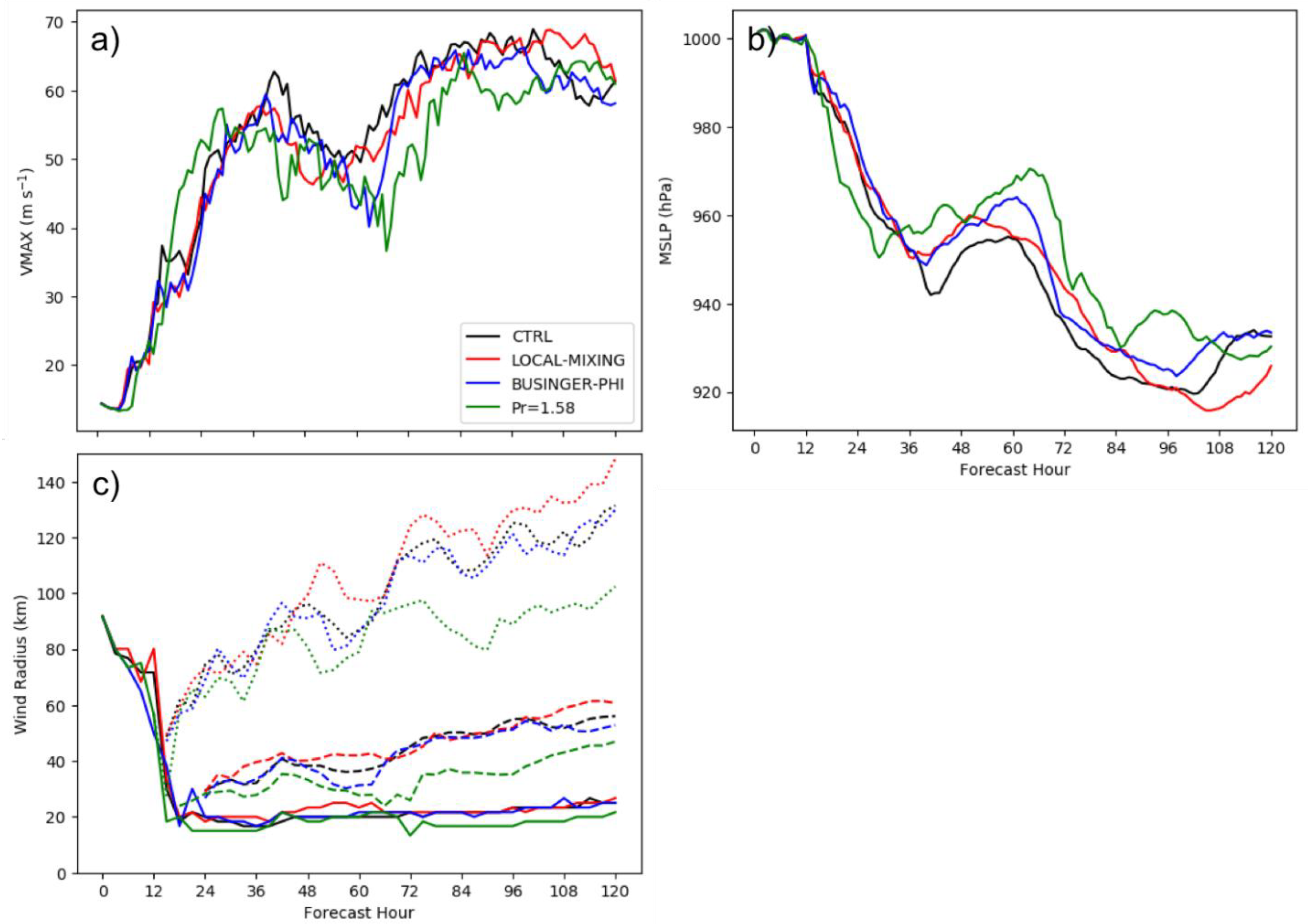
• Has smaller radii of maximum, 64-, and 34-kt winds, possibly due to the weaker enthalpy fluxes, with the largest impact on the 34-kt wind radius;
• Is more likely to undergo an initial period of rapid intensification, due to its smaller size;
• Reaches a weaker peak intensity due to the smaller enthalpy fluxes in the inner core.

Due to the way that the eddy diffusivities of momentum, heat, and moisture are calculated in the GFS-EDMF PBL (Equations (5)–(6)), the eddy diffusivity of momentum for a particular wind speed is unaffected by modifications to Pr, since Pr is only used to obtain the eddy diffusivities of heat and moisture from K_m. While K_m plays an important role in determining TC intensity and the potential for rapid intensification, it is far from the only important variable in the PBL scheme, as this study demonstrates.

Future work should focus on collecting additional observations of K_m and K_h in the TC PBL that can be used to determine Pr, possibly using Uncrewed Aircraft Systems equipped with turbulence probes. These additional measurements are needed to further explore the relationship between stability and Pr in the TC PBL, which may differ from that in the more readily-studied PBL over the land, as suggested by the CBLAST results. If subsequent measurements confirm that Pr in the TC PBL is unique, a Pr parameterization that accounts for this behavior could be developed. In addition to stability, such a parameterization might consider whether the vertical column is over land or over water and/or include a wind speed dependence to estimate Pr accurately across a variety of phenomena, including TCs. In addition, examining the TC response across a wider range of Pr, particularly at smaller values than those examined here (i.e., Pr < 0.8), would help to quantify the TC sensitivity to Pr more completely.

References

1. Stensrud, D.J. Parameterization Schemes: Keys to Understanding Numerical Weather Prediction Models; Cambridge University Press: Cambridge, UK, 2007; ISBN 978-0-521-12676-2. [Google Scholar]
2. Riehl, H. A Model of Hurricane Formation. J. Appl. Phys. 1950, 21, 917–925. [Google Scholar] [CrossRef]
3. Kleinschmidt, E. Grundlagen einer Theorie der tropischen Zyklonen. Arch. Für Meteorol. Geophys. Bioklimatol. Ser. A 1951, 4, 53–72. [Google Scholar] [CrossRef]
4. Malkus, J.S.; Riehl, H. On the Dynamics and Energy Transformations in Steady-State Hurricanes. Tellus 1960, 12, 1–20. [Google Scholar] [CrossRef] [Green Version]
5. Emanuel, K. 100 Years of Progress in Tropical Cyclone Research. Meteorol. Monogr. 2018, 59, 15.1–15.68. [Google Scholar] [CrossRef]
6. Bernardet, L.; Tallapragada, V.; Bao, S.; Trahan, S.; Kwon, Y.; Liu, Q.; Tong, M.; Biswas, M.; Brown, T.; Stark, D.; et al. Community Support and Transition of Research to Operations for the Hurricane Weather Research and Forecasting Model. Bull. Am. Meteorol. Soc. 2015, 96, 953–960. [Google Scholar] [CrossRef]
7. Yablonsky, R.M.; Ginis, I.; Thomas, B.; Tallapragada, V.; Sheinin, D.; Bernardet, L. Description and Analysis of the Ocean Component of NOAA’s Operational Hurricane Weather Research and Forecasting Model (HWRF). J. Atmos. Ocean. Technol. 2015, 32, 144–163. [Google Scholar] [CrossRef] [Green Version]
8. Biswas, M.K.; Bernardet, L.; Abarca, S.; Ginis, I.; Grell, E.; Kalina, E.; Kwon, Y.; Liu, B.; Liu, Q.; Marchok, T.; et al. Hurricane Weather Research and Forecasting (HWRF) Model: 2017 Scientific Documentation. Dev. Testbed Cent. 2018. [Google Scholar] [CrossRef]
9. Mehra, A.; Tallapragada, V.; Zhang, Z.; Liu, B.; Zhu, L.; Wang, W.; Kim, H.-S. Advancing the State of the Art in Operational Tropical Cyclone Forecasting at Ncep. Trop. Cyclone Res. Rev. 2018, 7, 51–56. [Google Scholar] [CrossRef]
10. Han, J.; Bretherton, C.S. TKE-Based Moist Eddy-Diffusivity Mass-Flux (EDMF) Parameterization for Vertical Turbulent Mixing. Weather Forecast. 2019, 34, 869–886. [Google Scholar] [CrossRef]
11. Kepert, J.D. Choosing a Boundary Layer Parameterization for Tropical Cyclone Modeling. Mon. Weather Rev. 2012, 140, 1427–1445. [Google Scholar] [CrossRef] [Green Version]
12. Zhang, J.A.; Drennan, W.M. An Observational Study of Vertical Eddy Diffusivity in the Hurricane Boundary Layer. J. Atmos. Sci. 2012, 69, 3223–3236. [Google Scholar] [CrossRef]
13. Bu, Y.P.; Fovell, R.G.; Corbosiero, K.L. The Influences of Boundary Layer Mixing and Cloud-Radiative Forcing on Tropical Cyclone Size. J. Atmos. Sci. 2017, 74, 1273–1292. [Google Scholar] [CrossRef] [Green Version]
14. Braun, S.A.; Tao, W.-K. Sensitivity of High-Resolution Simulations of Hurricane Bob (1991) to Planetary Boundary Layer Parameterizations. Mon. Weather Rev. 2000, 128, 3941–3961. [Google Scholar] [CrossRef] [Green Version]
15. Smith, R.K.; Thomsen, G.L. Dependence of Tropical-Cyclone Intensification on the Boundary-Layer Representation in a Numerical Model. Q. J. R. Meteorol. Soc. 2010, 136, 1671–1685. [Google Scholar] [CrossRef]
16. Zhang, J.A.; Marks, F.D.; Montgomery, M.T.; Lorsolo, S. An Estimation of Turbulent Characteristics in the Low-Level Region of Intense Hurricanes Allen (1980) and Hugo (1989). Mon. Weather Rev. 2011, 139, 1447–1462. [Google Scholar] [CrossRef] [Green Version]
17. Zhang, J.A.; Gopalakrishnan, S.; Marks, F.D.; Rogers, R.F.; Tallapragada, V. A Developmental Framework for Improving Hurricane Model Physical Parameterizations Using Aircraft Observations. Trop. Cyclone Res. Rev. 2012, 1, 419–429. [Google Scholar] [CrossRef]
18. Gopalakrishnan, S.G.; Marks, F.; Zhang, J.A.; Zhang, X.; Bao, J.-W.; Tallapragada, V. A Study of the Impacts of Vertical Diffusion on the Structure and Intensity of the Tropical Cyclones Using the High-Resolution HWRF System. J. Atmos. Sci. 2013, 70, 524–541. [Google Scholar] [CrossRef]
19. Zhang, J.A.; Nolan, D.S.; Rogers, R.F.; Tallapragada, V. Evaluating the Impact of Improvements in the Boundary Layer Parameterization on Hurricane Intensity and Structure Forecasts in HWRF. Mon. Weather Rev. 2015, 143, 3136–3155. [Google Scholar] [CrossRef]
20. Zhang, J.A.; Rogers, R.F.; Tallapragada, V. Impact of Parameterized Boundary Layer Structure on Tropical Cyclone Rapid Intensification Forecasts in HWRF. Mon. Weather Rev. 2017, 145, 1413–1426. [Google Scholar] [CrossRef]
21. Zhang, J.A.; Rogers, R.F. Effects of Parameterized Boundary Layer Structure on Hurricane Rapid Intensification in Shear. Mon. Weather Rev. 2019, 147, 853–871. [Google Scholar] [CrossRef]
22. Tallapragada, V.; Kieu, C.; Kwon, Y.; Trahan, S.; Liu, Q.; Zhang, Z.; Kwon, I.-H. Evaluation of Storm Structure from the Operational HWRF during 2012 Implementation. Mon. Weather Rev. 2014, 142, 4308–4325. [Google Scholar] [CrossRef]
23. Zhang, J.A.; Kalina, E.A.; Biswas, M.K.; Rogers, R.F.; Zhu, P.; Marks, F.D. A Review and Evaluation of Planetary Boundary Layer Parameterizations in Hurricane Weather Research and Forecasting Model Using Idealized Simulations and Observations. Atmosphere 2020, 11, 1091. [Google Scholar] [CrossRef]
24. Wang, W.; Sippel, J.A.; Abarca, S.; Zhu, L.; Liu, B.; Zhang, Z.; Mehra, A.; Tallapragada, V. Improving NCEP HWRF Simulations of Surface Wind and Inflow Angle in the Eyewall Area. Weather Forecast. 2018, 33, 887–898. [Google Scholar] [CrossRef]
25. Vickers, D.; Mahrt, L. Evaluating Formulations of Stable Boundary Layer Height. J. Appl. Meteorol. 2004, 43, 1736–1749. [Google Scholar] [CrossRef] [Green Version]
26. Gall, R.; Franklin, J.; Marks, F.; Rappaport, E.N.; Toepfer, F. The Hurricane Forecast Improvement Project. Bull. Am. Meteorol. Soc. 2013, 94, 329–343. [Google Scholar] [CrossRef]
27. Bao, J.-W.; Gopalakrishnan, S.G.; Michelson, S.A.; Marks, F.D.; Montgomery, M.T. Impact of Physics Representations in the HWRFX on Simulated Hurricane Structure and Pressure–Wind Relationships. Mon. Weather Rev. 2012, 140, 3278–3299. [Google Scholar] [CrossRef] [Green Version]
28. Tang, J.; Zhang, J.A.; Kieu, C.; Marks, F.D. Sensitivity of Hurricane Intensity and Structure to Two Types of Planetary Boundary Layer Parameterization Schemes in Idealized HWRF Simulations. Trop. Cyclone Res. Rev. 2018, 7, 201–211. [Google Scholar] [CrossRef]
29. Troen, I.B.; Mahrt, L. A Simple Model of the Atmospheric Boundary Layer; Sensitivity to Surface Evaporation. Bound.-Layer Meteorol. 1986, 37, 129–148. [Google Scholar] [CrossRef]
30. Hong, S.-Y.; Pan, H.-L. Nonlocal Boundary Layer Vertical Diffusion in a Medium-Range Forecast Model. Mon. Weather Rev. 1996, 124, 2322–2339. [Google Scholar] [CrossRef] [Green Version]
31. Han, J.; Witek, M.L.; Teixeira, J.; Sun, R.; Pan, H.-L.; Fletcher, J.K.; Bretherton, C.S. Implementation in the NCEP GFS of a Hybrid Eddy-Diffusivity Mass-Flux (EDMF) Boundary Layer Parameterization with Dissipative Heating and Modified Stable Boundary Layer Mixing. Weather Forecast. 2016, 31, 341–352. [Google Scholar] [CrossRef]
32. Dyer, A.J.; Hicks, B.B. Flux-Gradient Relationships in the Constant Flux Layer. Q. J. R. Meteorol. Soc. 1970, 96, 715–721. [Google Scholar] [CrossRef]
33. Jordan, C.L. Mean Soundings for the West Indies Area. J. Meteorol. 1958, 15, 91–97. [Google Scholar] [CrossRef] [Green Version]
34. Wang, Y. An Inverse Balance Equation in Sigma Coordinates for Model Initialization. Mon. Weather Rev. 1995, 123, 482–488. [Google Scholar] [CrossRef] [Green Version]
35. Businger, J.A.; Wyngaard, J.C.; Izumi, Y.; Bradley, E.F. Flux-Profile Relationships in the Atmospheric Surface Layer. J. Atmos. Sci. 1971, 28, 181–189. [Google Scholar] [CrossRef]
36. Biswas, M.K.; Stark, D.; Carson, L. GFDL Vortex Tracker Users’ Guide V3.9a 2018.
37. Kaplan, J.; DeMaria, M. Large-Scale Characteristics of Rapidly Intensifying Tropical Cyclones in the North Atlantic Basin. Weather Forecast. 2003, 18, 1093–1108. [Google Scholar] [CrossRef] [Green Version]
38. Cione, J.J.; Kalina, E.A.; Zhang, J.A.; Uhlhorn, E.W. Observations of Air–Sea Interaction and Intensity Change in Hurricanes. Mon. Weather Rev. 2013, 141, 2368–2382. [Google Scholar] [CrossRef]
39. Cione, J.J.; Bryan, G.H.; Dobosy, R.; Zhang, J.A.; de Boer, G.; Aksoy, A.; Wadler, J.B.; Kalina, E.A.; Dahl, B.A.; Ryan, K.; et al. Eye of the Storm: Observing Hurricanes with a Small Unmanned Aircraft System. Bull. Am. Meteorol. Soc. 2020, 101, E186–E205. [Google Scholar] [CrossRef]
40. Hill, K.A.; Lackmann, G.M. Influence of Environmental Humidity on Tropical Cyclone Size. Mon. Weather Rev. 2009, 137, 3294–3315. [Google Scholar] [CrossRef]
41. Sun, Y.; Zhong, Z.; Li, T.; Yi, L.; Hu, Y.; Wan, H.; Chen, H.; Liao, Q.; Ma, C.; Li, Q. Impact of Ocean Warming on Tropical Cyclone Size and Its Destructiveness. Sci. Rep. 2017, 7, 8154. [Google Scholar] [CrossRef]
42. Emanuel, K.A. The Finite-Amplitude Nature of Tropical Cyclogenesis. J. Atmos. Sci. 1989, 46, 3431–3456. [Google Scholar] [CrossRef] [Green Version]
43. Chen, D.Y.-C.; Cheung, K.K.W.; Lee, C.-S. Some Implications of Core Regime Wind Structures in Western North Pacific Tropical Cyclones. Weather Forecast. 2011, 26, 61–75. [Google Scholar] [CrossRef]
44. Carrasco, C.A.; Landsea, C.W.; Lin, Y.-L. The Influence of Tropical Cyclone Size on Its Intensification. Weather Forecast. 2014, 29, 582–590. [Google Scholar] [CrossRef] [Green Version]
45. Fudeyasu, H.; Ito, K.; Miyamoto, Y. Characteristics of Tropical Cyclone Rapid Intensification over the Western North Pacific. J. Clim. 2018, 31, 8917–8930. [Google Scholar] [CrossRef]
46. Ma, Z.; Liu, B.; Mehra, A.; Abdolali, A.; van der Westhuysen, A.; Moghimi, S.; Vinogradov, S.; Zhang, Z.; Zhu, L.; Wu, K.; et al. Investigating the Impact of High-Resolution Land–Sea Masks on Hurricane Forecasts in HWRF. Atmosphere 2020, 11, 888. [Google Scholar] [CrossRef]
47. Liu, B.; Kim, H.-S.; Rosen, D.; Shin, J.; Thomas, B.; Sheinin, D.; Dong, J.; Zhu, L.; Zhang, C.; Wang, W.; et al. The HAFSv0.1A HFIP Real-Time Parallel Experiment: A Regional and Ocean-Coupled Configuration 2020. Available online: www.hfip.org/events/annual_meeting_nov_2020/index.php (accessed on 20 February 2021).
Figure 1. Time series of (a) maximum 10-m wind speed (b) minimum mean sea-level pressure, and (c) radius of maximum wind (solid lines), 64-kt wind (dashed lines), and 34-kt wind (dotted lines) at 10-m height for the CTRL (black), LOCAL-MIXING (red), BUSINGER-PHI (blue), and Pr = 1.58 (green) simulations.
Atmosphere 12 00284 g001
Figure 2. Storm-centered contour plots of the stability parameter (z1/L) in the CTRL run at (a) 72 h, (b) 96 h, and (c) 120 h. The black lines indicate the area of 34-, 50-, and 64-kt winds.
Atmosphere 12 00284 g002
Figure 3. Contour plots of the (a) difference between the sea-surface temperature (SST) and the air temperature at the lowest model level (dT = SST-TLML) in the CTRL run and (bd)) the percentage change in dT relative to the CTRL run in the (b) LOCAL-MIXING, (c) BUSINGER-PHI, and (d) Pr = 1.58 experiments at t = 120 h. The black/green lines indicate the area of 34-, 50-, and 64-kt winds.
Atmosphere 12 00284 g003
Figure 4. Contour plots of (a) the difference between the water vapor mixing ratio at the sea surface and the mixing ratio at the lowest model level (dq = qSST-qLML) in the CTRL run and (bd)) the percentage change in dq relative to the CTRL run in the (b) LOCAL-MIXING, (c) BUSINGER-PHI, and (d) Pr = 1.58 experiments at t = 120 h. The black/green lines indicate the area of 34-, 50-, and 64-kt winds.
Atmosphere 12 00284 g004
Figure 5. Contour plots of (a) the total enthalpy flux in the CTRL run and (b–d)) the percentage change in the total enthalpy flux relative to the CTRL run in the (b) LOCAL-MIXING, (c) BUSINGER-PHI, and (d) Pr = 1.58 experiments at t = 120 h. The black/green lines indicate the area of 34-, 50-, and 64-kt winds.
Atmosphere 12 00284 g005
Figure 6. The relationship between Pr (Km/Kh) and the additive inverse of the stability parameter (-z1/L) within the innermost HWRF domain for winds weaker than 34 kt (gray dots), 34–64 kt (yellow dots), and stronger than 64 kt (red dots) in the (a) CTRL, (b) LOCAL-MIXING, and (c) BUSINGER-PHI simulations at t = 120 h. The relationships implied by the stability functions from Dyer (black lines) and Businger (blue lines) are also shown.
Atmosphere 12 00284 g006
Figure 7. Storm-centered, azimuthally-averaged Kh in the (a) CTRL, (b) LOCAL-MIXING, (c) BUSINGER-PHI, and (d) Pr = 1.58 simulations at t = 120 h. The maximum (solid line), 64-kt (dashed line), and 34-kt (dotted line) wind radii of the azimuthally-averaged wind field are also shown.
Atmosphere 12 00284 g007
Figure 8. Storm-centered, azimuthally-averaged Pr in the (a) CTRL, (b) LOCAL-MIXING, (c) BUSINGER-PHI, and (d) Pr = 1.58 simulations at t = 120 h. The maximum (solid line), 64-kt (dashed line), and 34-kt (dotted line) wind radii of the azimuthally-averaged wind field are also shown.
Atmosphere 12 00284 g008