Chemical and Optical Characteristics and Sources of PM_2.5 Humic-Like Substances at Industrial and Suburban Sites in Changzhou, China

Abstract

The chemical and optical properties and sources of atmospheric PM_2.5 humic-like substances (HULIS) were investigated from October to December 2016 in both industrial and suburban areas in Changzhou, China, during polluted and fair days. The average PM_2.5 concentration in the industrial region was 113.06 (±64.3) μg m⁻³, higher than 85.27 (±41.56) μg m⁻³ at the suburban site. The frequency of polluted days was significantly higher in the industrial region. In contrast, the chemical compositions of PM_2.5 at the two sampling sites exhibited no statistically significant differences. Rapidly increased secondary inorganic ions (SNA = NH₄⁺ + SO₄²⁻ + NO₃⁻) concentrations suggested secondary formation played an important role in haze formation. The daily mean concentration of humic-like substance (HULIS) was 1.8–1.9 times that of HULIS-C (the carbon content of HULIS). Our results showed that HULIS accounted for a considerable fraction of PM_2.5 (industrial region: 6.3% vs. suburban region: 9.4%). There were no large differences in the mass ratios of HULIS-C/WSOC at the two sites (46% in the industrial region and 52% in the suburban region). On average, suburban HULIS-C constituted 35.1% of organic carbon (OC), higher than that (21.1%) in the industrial region. Based on different MAE (mass absorption efficiency) values under different pollution levels, we can infer that the optical properties of HULIS varied with PM levels. Moreover, our results showed no distinct difference in E₂/E₃ (the ratio of light absorbance at 250 nm to that at 365 nm) and AAE_300–400 (Absorption Angstrom Exponent at 300–400 nm) for HULIS and WSOC. the MAE₃₆₅ (MAE at 365 nm) value of HULIS-C was different under three PM_2.5 levels (low: PM_2.5 < 75 μg m⁻³, moderate: PM_2.5 = 75–150 μg m⁻³, high: PM_2.5 > 150 μg m⁻³), with the highest MAE₃₆₅ value on polluted days in the industrial region. Strong correlations between HULIS-C and SNA revealed that HULIS might be contributed from secondary formation at both sites. In addition, good correlations between HULIS-C with K⁺ in the industrial region implied the importance of biomass burning to PM_2.5-bound HULIS. Three common sources of HULIS-C (i.e., vehicle emissions, biomass burning, and secondary aerosols) were identified by positive matrix factorization (PMF) for both sites, but the contributions were different, with the largest contribution from biomass burning in the industrial region and secondary sources in the suburban region, respectively. The findings presented here are important in understanding PM_2.5 HULIS chemistry and are valuable for future air pollution control measures.

1. Introduction

Brown carbon (BrC), a class of organic matter in aerosols, has strong light absorption in the UV–vis region (300–700 nm). Humic-like substances (HULIS), a complex group of organics, account for an important fraction of BrC [1]. HULIS has strong light-absorbing ability in the near-UV range of 200–400 nm, thus playing a significant role in atmospheric radiative forcing and climate change. Specific absorbance can also be considered as an effective indicator of the origin of HULIS in ambient particulate matter (PM) [2]. HULIS might also threaten human health owing to the production of reactive oxygen species (ROS) or via complexation with transition metals (e.g., Fe, Mn, Cu) [3,4,5]. Recently, many studies have focused on the ROS-generation potential of HULIS in PM_2.5 [6,7]. HULIS may also act as photosensitizers to participate in atmospheric photochemical reactions. HULIS has not been studied thoroughly, and knowledge of HULIS optical properties, chemical structural characteristics, and sources is limited but important in assessing its effects on air quality, climate, and human health [8].

As a class of highly complex macromolecular compounds in ambient PM, HULIS consists of poly-conjugated structural elements with carboxyl, hydroxyl, and carbonyl polar groups. HULIS can originate from biomass burning (BB) and secondary formation processes such as atmospheric photochemical reactions or aqueous-phase oxidation [9,10,11,12]. Emission sources and secondary formation of HULIS in the atmospheric environment are influenced by seasons [10,13], usually intense BB emissions in winter and significant secondary processes in summer. Furthermore, the chemical and optical characteristics of HULIS might vary in different locations owing to different emission scenarios [14]. To date, studies on the quantitation of HULIS sources are still limited, and comparison of fine particle (PM_2.5) properties between suburban and industrial regions is also relatively scarce [15], especially due to technical difficulties of sample collection in highly-polluted industrial regions. The individual as well as combined influences of various factors on the formation of HULIS in different regions needs further investigation since assessment of health effects associated with HULIS should address their chemical composition and optical properties instead of only focusing on the mass concentration. So far, there are few HULIS reports in industrial regions. Therefore, the present study aims to study the characteristics of HULIS in both suburban and industrial environments.

In this work, PM_2.5 samples were collected at two sites (located in industrial and suburban regions) in Changzhou, a neighborhood city of Shanghai in the Yangtze River Delta (YRD) region, China. A very recent report showed that Changzhou suffers from severe air pollution [16]. Details of the sampling sites are presented in Figure S1 in the Supplementary Materials. The industrial site is located in the northern part of Changzhou, where numerous industrial plants can emit a large amount of gaseous pollutants and other particulate carbonaceous species. The sampler was set on the roof of a private house, about 15 m above the ground. The suburban site was located in the southern part, a representative area with mixed residential, educational, and traffic activities. The chemical and optical properties of PM_2.5 HULIS at the two sites were measured by using a suite of instruments, including a TOC analyzer, UV–vis spectrometer, and high performance liquid chromatography (HPLC). The purposes of this study are (1) to compare the mass levels of HULIS at the two sites, (2) to systematically investigate the regional variations and influences of weather conditions on the mass and optical properties of HULIS, and (3) to identify the sources of HULIS. The results of this study would provide valuable information for environmental policy makers for sustainable control policies and strategies that could help to abate air pollution and thereby reduce its associated human health risks.

2. Experimental Section

2.1. Sample Collection

A total of 60 22-h PM_2.5 samples from the suburban site and 74 samples from the industrial site were synchronously collected on a prebaked (at 500 °C) quartz fiber filter (20.3 cm × 25.4 cm; Whatman QM-A, Whatman, Maidstone, UK) from 8 October to 28 December in 2016. We used a high-volume air sampler (KB-1000, Qingdao Jinsida Co., Ltd., Qingdao, China) with an air flow rate of 1.05 m³·min⁻¹ to collect the PM_2.5 samples. After collection, filters were wrapped with aluminum foil, sealed in a zipped bag, transported to the laboratory in a cooler with ice packs, and immediately stored in a refrigerator at −18 °C prior to analysis.

In this article, the sampling period is divided into polluted days (daily PM_2.5 > 75 µg m⁻³) and fair days (daily PM_2.5 ≤ 75 µg m⁻³) based on the national daily air quality standard in China (NAAQS) Grade II of PM_2.5 (75 µg m⁻³), as suggested by Liu et al [17].

2.2. Chemical Analyses

2.2.1. WSOC, HULIS-C, and HULIS

One quarter of each filter was dissolved in MilliQ water (50 mL) to obtain water extracts of PM_2.5 (20 mL for water-soluble organic carbon (WSOC) and 30 mL for HULIS). The details of the pretreatment procedures were previously described [18,19]. WSOC was determined using a total organic carbon (TOC) analyzer (TOC–VCPH, Shimadzu, Japan) based on a combustion–oxidation, nondispersive infrared absorption method. The 30 mL water extract was evenly divided into two portions for HULIS and HULIS-C analyses. A solid-phase extraction (SPE) cartridge (CNW Poly-Sery HLB, 60 mg/cartridge) was used to isolate HULIS from the water extracts. The original SPE cartridge was first rinsed with 1 mL MilliQ water and 3 mL methanol. The water extracts were acidified to pH = 2 using 1 mL of 0.01 M HCl and loaded on the cartridge, followed by washing with 1 mL MilliQ water. The HULIS sample was eluted with 3 mL methanol containing 2% ammonia (w/w). The resulting eluate was evaporated to dryness with ultrapure N₂ and re-dissolved in 2 mL MilliQ water for the quantification of HULIS mass and in 30 mL MilliQ water for determination of the HULIS-C fraction using the TOC analyzer. For HULIS quantification, an aliquot of 20 μL of the aqueous solution was injected into an HPLC system coupled to an evaporative light-scattering (ELSD3000) detector.

2.2.2. OC and EC

The concentrations of organic carbon (OC) and elemental carbon (EC) were analyzed by a thermal/optical carbon analyzer (Model 2001A, Desert Research Institute, Reno, Nevada, USA) following a thermal/optical reflectance (TOR) protocol. Briefly, a 1.45 cm² punch of each filter was heated stepwise at temperatures of 140 °C (OC₁), 280 °C (OC₂), 480 °C (OC₃), and 580 °C (OC₄) in a non-oxidizing helium atmosphere and at 580 °C (EC₁), 740 °C (EC₂), and 840 °C (EC₃) in a 2% oxygen/98% helium gas atmosphere. OC was calculated as OC₁ + OC₂ + OC₃ + OC₄ + OP and EC as EC₁ + EC₂ + EC₃ − OP, where OP is the optical pyrolyzed OC. By subtracting the blank value from the sample concentration, the measured OC and EC concentrations could be corrected.

2.2.3. Water-Soluble Ions

A water extract of PM_2.5 for water-soluble inorganic ions (WSIIs) was obtained following the same method as the WSOC pretreatment. The concentrations of three anions (Cl⁻, NO₃⁻, and SO₄²⁻) and five cations (Na⁺, NH₄⁺, K⁺, Mg²⁺, and Ca²⁺) were measured by ion chromatography (IC) (Thermo Scientific Dionex Aquion IC, Shanghai, China). An anion column (4 mm × 250 mm, Dionex AS23, Thermo Fisher Scientific Inc., Waltham, MA, USA) was used to separate anions from the filtrate through the eluent (4.5 mmol·L⁻¹ Na₂CO₃ and 0.8 mmol·L⁻¹ NaHCO₃) at 0.8 mL·min⁻¹. A cation column (4 mm × 250 mm, Dionex CS12, Thermo Fisher Scientific Inc., Waltham, MA, USA) was used to separate the cations in the filtrate through the mobile phase (18 mmol·L⁻¹ methanesulfonic acid). The flow rate was 0.8 mL·min⁻¹ at 25 °C. In addition, oxalate and formate could also be quantified in the same anion run with a Dionex AS23 column replaced by a Dionex AS11 column.

2.2.4. Heavy Metals

In this procedure, 1/16 of each filter was placed into a Teflon digestion vessel. Then, a 10 mL mixture of HNO₃ and HCl (1:1, v:v) was added, and the Teflon vessel was placed in a microwave digestor (XT-9900A, Shanghai Xintuo Co., Shanghai, China) for dissolution [20]. Finally, the mixture was heated to 130 °C until it was completely dried and was then diluted to 25 mL with ultrapure water. The concentrations of 14 heavy metals (Pb, Fe, Al, Zn, Ag, As, Cd, Co, Cr, Cu, Mn, Ni, Se, and V) were analyzed by an inductively coupled plasma optical emission spectrometer (ICP–OES) as described in our previous work [19,21].

2.2.5. Water-Soluble Organic Matter (WSOM)

We also used an Aerodyne soot particle aerosol mass spectrometer (SP–AMS) to analyze the chemical composition of WSOM [22]. Note SP–AMS is an advanced instrument that is often deployed for online and real-time measurement of fine particle composition [23,24]; recently, we successfully developed the technique by using this instrument for offline analysis of filter extracts [25,26]. The SP–AMS can provide the mass spectrum of WSOM in the form of 70 ev electron impact (EI)-ionized fragments of the organics. Here, concentrations of some SP–AMS tracer ions indicative of specific sources were used for correlation analysis with HULIS-C (see Section 3.4.3).

2.3. Light Absorption Coefficients of HULIS and WSOC

Light absorption spectra of water extracts of aerosols (WSOC and HULIS) were recorded by a Shimadzu UV-2600 spectrophotometer from 200 to 700 nm with a 1 cm quartz cell. The absorption coefficient at wavelength λ (Abs_λ) [27,28,29,30] can be calculated according to Equation (1):

$$Ab{s}_{\lambda }=(A_{\lambda }-A_{700})V_L\ln 10/(V_{air}\cdot L)$$

(1)

where Abs_λ is expressed in the unit of M m⁻¹, and A_λ refers to absorbance at wavelength λ. A₇₀₀ is the light absorbance at 700 nm, a base value to eliminate the errors caused by baseline fluctuation. V_air corresponds to the volume of air sampled (m³), V_L refers to the volume of the extraction (mL), L is the optical path length of the lamp (0.01 m).

The mass absorption efficiency (MAE_λ, m²·g⁻¹) at wavelength λ was used to characterize the optical property, calculated by dividing Abs_λ by the mass concentration of WSOC, and expressed by the following equation [29,31]:

MAE_λ = Abs_λ/C

(2)

Here, C corresponds to either the WSOC or HULIS-C content in air (μg m⁻³).

The absorption Angstrom exponent (AAE) was then used to describe the dependence of the light absorbption by HULIS and WSOC on wavelength, as expressed by the following equation [29,31]:

$$AAE=\ln (\frac{MA{E}_{{\lambda }_1}}{MA{E}_{\lambda 2}})\times \ln (\frac{{\lambda }_2}{{\lambda }_1})$$

(3)

Since light absorbance of HULIS mainly occurs in range of 300–400 nm, AAE_(300–400) was calculated and used in this study.

2.4. PMF Analysis

Positive matrix factorization (PMF) was conducted to quantify PM_2.5 and HULIS-C sources [32]. PMF does not require the source profile prior to analysis and has no limitation on the number of sources, so, it is an effective receptor model and has been widely used in source apportionment of PM. EPA PMF software (version 5.0) was used in this work. The detailed principles of PMF can be obtained elsewhere [15].

We used a total of 19 measured chemical components for PMF analysis, including carbonaceous components (HULIS-C, HULIS, WSOC, OC, EC), ions (oxalate, Cl⁻, NO₃⁻, SO₄²⁻, NH₄⁺, K⁺, Mg²⁺, Ca²⁺), and six heavy metals (Pb, Fe, Al, As, Cu, and Zn). It is worth noting that metal elements were added in the operation of PMF in order to analyze HULIS sources more accurately. Since K⁺ has multiple emission sources, such as soil dust, sea salt, and biomass burning [33], K⁺ was replaced by BB-corrected K⁺ (K_b = K-0.35Fe) for PMF analysis as suggested by Pachon [34]. Sodium might have high blank values on the quartz filter, so we did not include it in the PMF analysis.

Finally, we selected a four-factor solution for the suburban region and a five-factor solution for the industrial region as the final optimal PMF results by performing 100 bootstrap runs, with more than 90% of the runs producing the chosen solutions. Theoretical Q_true and Q_robust displayed a <5% difference. As stated before, the extra modeling uncertainty was set to 5%. Scaled residuals of >95% data were in the range of −3 to 3. A good correlation was found between model-apportioned HULIS-C (industrial: r = 0.97; suburban: r = 0.92), OC (industrial: r = 0.90; suburban: 0.90) and WSOC (industrial: r = 0.91; suburban: r = 0.92) with real measured concentrations.

2.5. Quality Assurance and Quality Control (QA/QC)

All analytical methods were subjected to strict quality assurance and quality control. Blank filters were analyzed, and the results were used for correcting sample concentrations. Method detection limits (MDLs) were defined as three times the standard deviations of the blank sample. The MDLs for EC and OC were 0.2 μg m⁻³ and 0.6 μg m⁻³, respectively. The MDLs of WSIIs (Cl⁻, NO₃⁻, SO₄²⁻, Na⁺, NH₄⁺, K⁺, Mg²⁺, and Ca²⁺) were lower than 0.08 μg m⁻³. Instrument stability and accuracy of methods were estimated by calculating the relative standard deviation (RSD) of one selected sample analyzed ten times. The RSDs were all in the range of 0–10% for all species, including OC, EC, WSIIs, and heavy metals. The correlation coefficients (r²) for linear regressions of the calibration curves exceeded 0.995.

For the PMF analysis, the uncertainty of an individual species was calculated as $\sqrt{{(\mathrm{RSD}\times \mathrm{concentration})}^2+{\mathrm{MDLs}}^2}$ according to the manual. When the concentration was below the MDLs, it was replaced by 1/2 MDLs, and the corresponding uncertainty was set to 5/6 MDLs.

3. Results and Discussion

3.1. Comparisons of PM_2.5 and Its Constituents at the Two Sites

The average daily concentrations of PM_2.5, carbonaceous species (OC, EC, WSOC, HULIS-C, et al.), inorganic ions (such as SO₄²⁻, NO₃⁻, NH₄⁺, K⁺, et al.), and selected mass ratios of these species during polluted and fair days are summarized in

Table 1. Mean concentration of PM_2.5 and its constituents (in µg m⁻³) with one standard deviation (Std) and mass ratios and fractions of selected species at the two sites during polluted and fair days.

Constitutents	Industrial Region			Suburban Region
	Fair (n = 24)	Polluted (n = 50)	All (n = 74)	Fair (n = 29)	Polluted (n = 31)	All (n = 60)
	Average ± Std	Average ± Std	Average ± Std	Average ± Std	Average ± Std	Average ± Std
PM2.5 and its carbonaceous contents (μg m−3)
PM2.5	52.07 ± 12.46	142.33 ± 58.33	113.06 ± 64.3	51.82 ± 12.90	116.57 ± 34.06	85.27 ± 41.56
OC	8.55 ± 3.15	21.75 ± 9.54	17.47 ± 10.14	7.27 ± 2.66	20.20 ± 7.90	13.95 ± 8.80
EC	2.28 ± 1.14	5.33 ± 3.05	4.34 ± 2.96	2.22 ± 0.83	4.19 ± 2.86	3.24 ± 2.35
HULIS	3.90 ± 1.14	7.46 ± 2.78	6.30 ± 2.90	5.33 ± 0.90	9.29 ± 2.29	7.38 ± 2.65
HULIS-C	2.03 ± 0.70	3.92 ± 1.46	3.31 ± 1.54	2.91 ± 0.49	5.02 ± 1.19	4.00 ± 1.40
WSOC	4.39 ± 0.98	8.78 ± 3.34	7.35 ± 3.47	5.50 ± 0.94	9.77 ± 2.71	7.70 ± 2.96
Water-soluble ions (μg m−3)
Na+	0.47 ± 0.22	0.79 ± 0.98	0.68 ± 0.83	1.55 ± 0.69	1.70 ± 0.51	1.63 ± 0.61
Cl−	1.17 ± 0.64	2.48 ± 1.56	2.05 ± 1.47	2.28 ± 1.04	5.11 ± 3.52	3.74 ± 2.99
K+	0.25 ± 0.08	0.51 ± 0.21	0.42 ± 0.21	0.46 ± 0.42	0.86 ± 0.89	0.67 ± 0.73
NO3−	4.99 ± 1.85	19.49 ± 11.35	14.79 ± 11.58	6.19 ± 2.65	20.46 ± 11.38	13.56 ± 11.00
SO42−	6.58 ± 1.63	13.77 ± 6.32	11.44 ± 6.26	8.19 ± 2.90	14.86 ± 5.17	11.64 ± 5.38
NH4+	4.81 ± 1.32	9.30 ± 2.99	7.85 ± 3.32	4.67 ± 1.54	9.86 ± 2.82	7.35 ± 3.46
formate	0.19 ± 0.10	0.45 ± 0.20	0.36 ± 0.21	0.60 ± 0.96	0.63 ± 0.59	0.61 ± 0.79
oxalate	0.20 ± 0.13	0.37 ± 0.21	0.32 ± 0.20	0.39 ± 0.99	0.42 ± 0.19	0.41 ± 0.70
Contributions
HULIS/HULIS-C	1.95 ± 0.15	1.91 ± 0.13	1.92 ± 0.14	1.83 ± 0.06	1.85 ± 0.10	1.84 ± 0.08
HULIS-C/WSOC (%)	45.8 ± 8.5	46.1 ± 9.8	46.0 ± 9.4	53.0 ± 2.3	52.0 ± 4.4	52.5 ± 3.5
HULIS-C/OC (%)	24.5 ± 5.2	19.4 ± 6.1	21.1 ± 6.3	.43.9 ± 13.3	27.0 ± 7.4	35.1 ± 13.6
HULIS/PM2.5 (%)	7.6 ± 1.8	5.6 ± 1.9	6.3 ± 2.1	10.7 ± 2.0	8.2 ± 1.4	9.4 ± 2.1
OC/EC	4.47 ± 2.06	5.06 ± 3.03	4.87 ± 2.77	3.57 ± 1.51	6.28 ± 3.23	4.97 ± 2.89

. Among all samples, 50 (67.6%) samples showed a high PM_2.5 level (>75 μg m⁻³) in the industrial area, while the number was only 31 (51.7%) of 60 in the suburban area, indicating the industrial area suffered more serious pollution. The average PM_2.5 concentrations for the collected samples were 113.06 ± 64.3 μg m⁻³ and 85.27 ± 41.56 μg m⁻³ in industrial and suburban regions, respectively. Consistent with our previous results for Changzhou [19], carbonaceous species and secondary inorganic ions (herein denoted as SNA, SNA = NH₄⁺ + SO₄²⁻ + NO₃⁻) were the major components. Although PM_2.5 and its chemical constituents were slightly higher in the industrial area than those in the suburban area, the relative mass fractions of HULIS-C in WSOC (industrial: 46.0%; suburban: 52.5%) were very similar at the two sites throughout the entire sampling period, similar to results for Hong Kong (53.4%) [7] and urban Shanghai (50%) [35]. A previous study [10] showed that the HULIS–C/WSOC ratio was generally within the range of 24–72%. On the contrary, the HULIS/PM_2.5 (8.7%) and HULIS-C/OC (35.1%) ratios at the suburban site were significantly higher than those (6.3% and 21.1%) in the industrial region. The HULIS-C/OC ratio was comparable to or higher than that observed in Guangzhou (17%) [36] and Xi’an (34.5%) [37], highlighting the significant contribution of HULIS-C to organic aerosol mass in our study. The linear regression line of HULIS vs. HULIS-C is plotted in Figure S2, showing the HULIS/HULIS-C ratios of 1.92 (industrial) and 1.84 (suburban), consistent with values in South China [36] and within the range reported before (1.8–2.3) [10,38]. The excellent correlation between HULIS-C (results from the TOC analyzer) and HULIS (results from HPLC–ELSD) reveals a good comparative performance of both methods.

In the industrial region, the average PM_2.5 mass concentration was 142.33 μg m⁻³ on polluted days, which was much higher (2.8 times) than that (52.07 μg m⁻³) on fair days, and 1.9 times the NAAQS Grade II. Further, concentrations of SNA (NO₃⁻, SO₄²⁻, and NH₄⁺) increased rapidly on polluted days with a factor of about 4~5, indicating the importance of secondary processes on haze formation. Relatively synchronous increases were found for other PM_2.5 species during polluted days, such as WSOC, OC, and their fractions in PM_2.5. At the suburban site, the OC/EC ratio (6.28) on polluted days was significantly higher than the value (3.57) on fair days, while in the industrial area, the difference was not that large (5.06 vs. 4.47).

The HULIS concentrations exhibited daily mean levels of 3.90 μg m⁻³ (fair) and 7.46 μg m⁻³ (polluted) in the industrial area, lower than those at the suburban area (fair: 5.33 μg m⁻³, polluted: 9.29 μg m⁻³). The average HULIS concentration (suburban: 7.38 and industrial: 6.30 μg m⁻³) was comparable with results for other urban cities (for example, 7.24 μg m⁻³ in Lanzhou) [10]. Both oxalate and formate exhibited slightly higher concentrations at the suburban site than those observed in the industrial area. It is known [39] that both formate and oxalate could come from secondary sources. Thus, we conclude that secondary sources likely contributed to HULIS more significantly in the suburban area than in the industrial region.

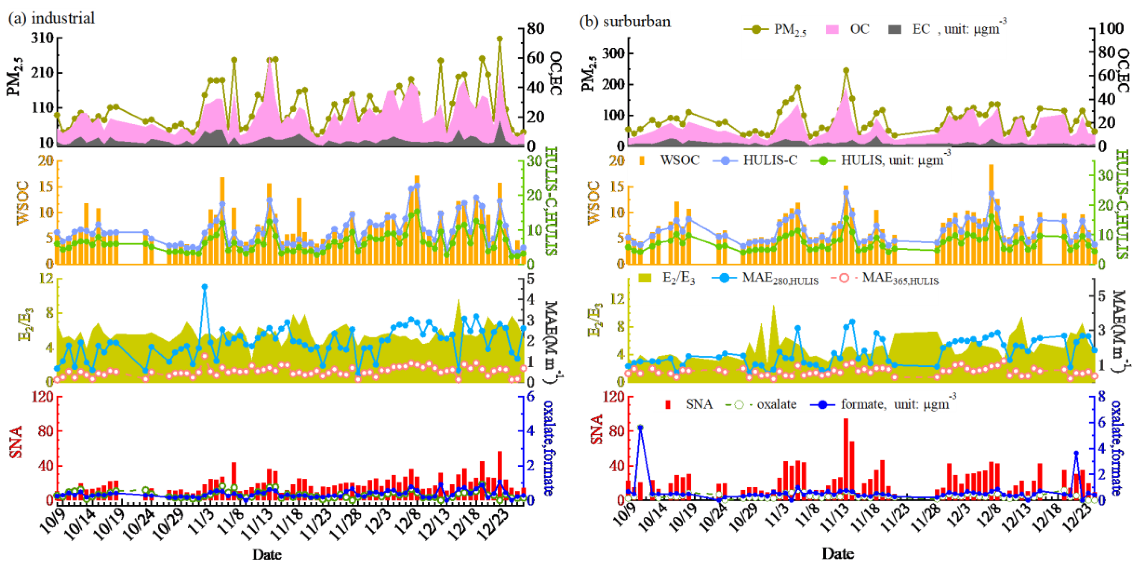
3.2. Temporal Variations of PM, HULIS, and Other Related Parameters

To obtain more detailed information, we examined the temporal variations of some species (Figure 1). Daily PM_2.5 concentrations ranged from 30 to 307.52 µg m⁻³ in the industrial region and from 35 to 245 µg m⁻³ in the suburban area during the sampling period. The peak PM_2.5 concentration (307.52 µg m⁻³) occurred on 12 December 2016, in the industrial region. During the entire sampling period, severely polluted days (PM_2.5 > 150 µg m⁻³) accounted for 12.5% of total sampling days in the industrial area. The daily average concentrations of PM_2.5 in the industrial area frequently exceeded 150 µg m⁻³ and even reached 300 µg m⁻³, which could tentatively be explained by the very complex processes that may take place during severely polluted episodes. For example, the mixing layer height decreases, and poor diffusion conditions or unfavorable conditions (such as high humidity or temperature, etc.) cause heavy pollution due to the accumulation of pollutants. More polluted days in the industrial region indicated that the PM_2.5 pollution was still very serious despite the implementation of stricter control measures in the industrial region.

As presented in Figure 1, in this study, except for a small number of samples, the majority of collected samples exhibited an OC/EC ratio >2.0, implying the importance of secondary organic aerosols across all fall–winter periods in Changzhou. SNA concentrations fluctuated more obviously than other species on severely polluted days, suggesting SNA plays important roles in the formation of haze [40]. Moreover, HULIS, HULIS-C, and WSOC concentrations varied in the range of 3.96–16.21, 2.19–8.64, and 4.02–19.22 µg m⁻³ in the suburban region and of 2.26–15.32, 1.14–7.72, and 2.52–17.17 µg m⁻³ in the industrial region. MAE₂₈₀ and MAE₃₆₅ of HULIS (defined as MAE_280,HULIS and MAE_365,HULIS) were in the range of 0.39–4.61 and 0.13–1.27 m² g⁻¹, with average values of 1.93 m² g⁻¹ and 0.52 m² g⁻¹ in the industrial region. Formate and oxalate concentrations varied little in the industrial region, but two peak formate concentrations appeared on 10 October and 21 December in the suburban region.

3.3. Light-Absorbing Characteristics of HULIS

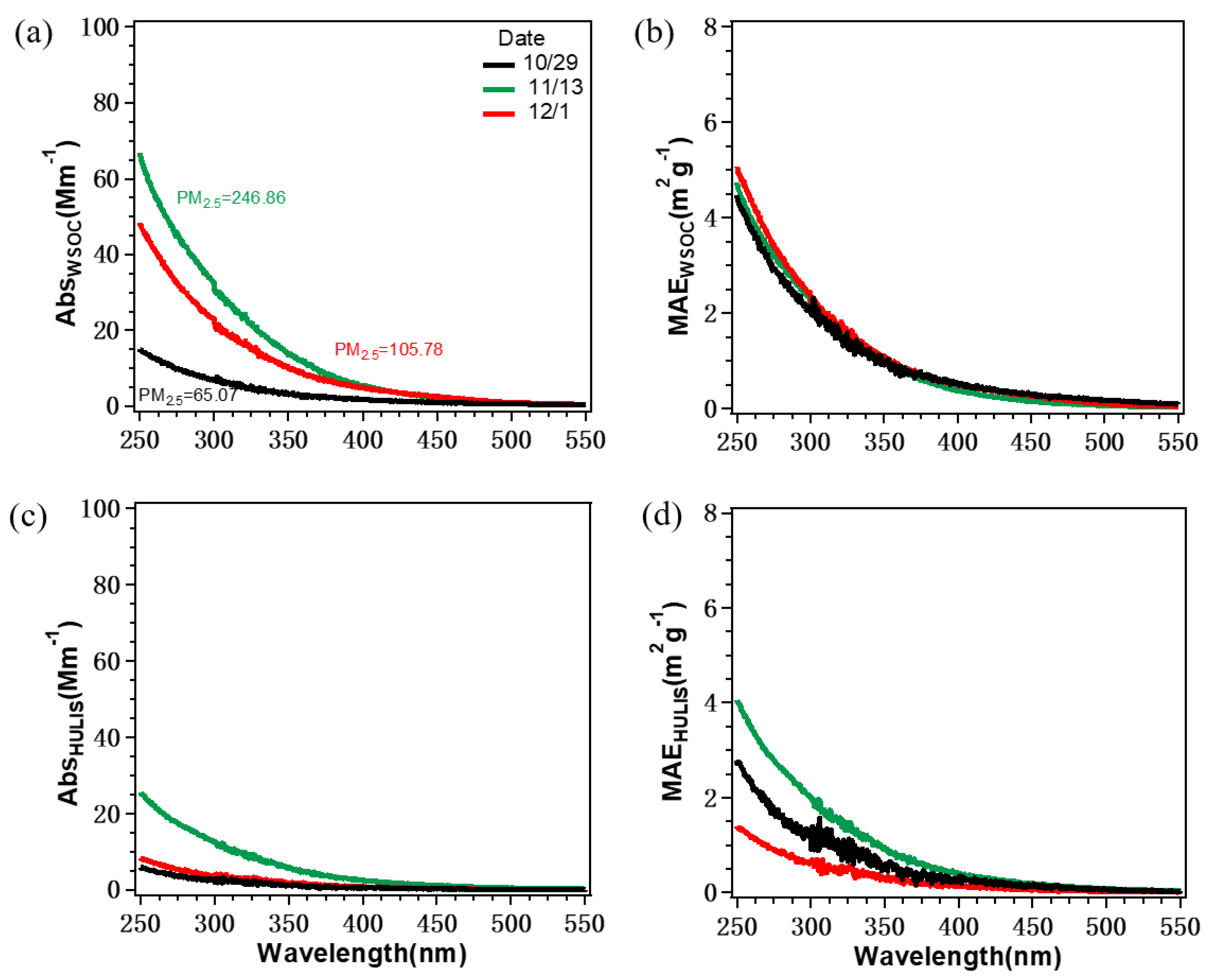
3.3.1. UV–Vis Spectra of HULIS

Figure 2 shows the UV–vis spectra (expressed by Abs) determined for WSOC and HULIS in the wavelength range of 250–550 nm in the industrial region. We selected three different pollution levels of PM_2.5 (low: PM_2.5 < 75 μg m⁻³, moderate: PM_2.5 = 75–150 μg m⁻³, high: PM_2.5 > 150 μg m⁻³) to illustrate its behavior. As can be seen, the overall wavelength dependences were similar, i.e., the Abs for both WSOC and HULIS (expressed by Abs_WSOC and Abs_HULIS) generally decreased as the wavelength increased. The HULIS had similar absorption patterns as WSOC, but they also exhibited distinct features. The decreased trend seemed to be smoother for Abs_HULIS than for Abs_WSOC; in other words, light-absorbing properties tended towards short wavelengths for WSOC, suggesting less aromaticity of WSOC compared to HULIS. As we know [30], MAE presented mass-normalized UV–vis spectra, namely, light absorbance per unit mass of HULIS-C or WSOC. As we can see from Figure 2, the normalized absorption intensities for WSOC (MAE_WSOC) were higher than those for the corresponding HULIS (MAE_HULIS). The finding contradicts with the results obtained previously for BB aerosols [41], which suggests higher MAE_HULIS than MAE_WSOC. Furthermore, the high PM_2.5 level exhibited an absolutely higher Abs value but nearly the same MAE_WSOC at all wavelengths, implying similar compositions regardless of the PM_2.5 levels. Different from MAE_WSOC, the wavelength dependence of MAE_HULIS was different for the three PM_2.5 levels, with the highest MAE_HULIS value for severely polluted days and the lowest at a moderate PM_2.5 concentration, indicating that the chemical and optical properties of HULIS were different under different pollution levels, and HULIS could contribute significantly to visibility degradation due to its strong light-absorbing properties. As we know [29], the chemical components and structure of HULIS from primary aerosols and secondary processes may well be different; as a result, MAE_HULIS values for different PM_2.5 levels were therefore different.

Likewise, Figure S3 shows the wavelength dependences of light absorbance for both WSOC and HULIS in the suburban region. The overall trend for Abs_HULIS was similar to that in the industrial region; nevertheless, the curve was not as smooth as that in the industrial region. Furthermore, the higher PM_2.5 level corresponded to higher Abs_HULIS and MAE_HULIS values at any wavelength, indicating higher absolute and relatively strong light absorption ability for HULIS by suburban ambient fine particles.

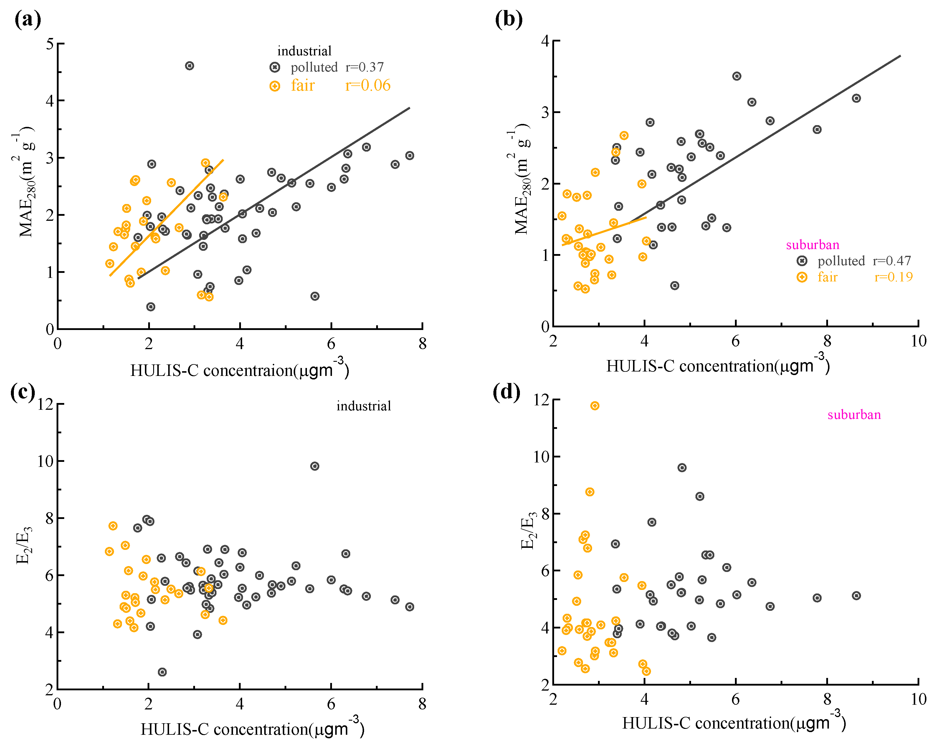
3.3.2. Optical Properties of HULIS

To assess the impact of water-soluble carbon (HULIS-C and WSOC) on light-absorption (340 nm and 365 nm, namely, Abs₃₄₀ andAbs₃₆₅), correlation analysis was conducted between Abs₃₆₅, Abs₃₄₀, and the WSOC concentration [27]. Good correlations between Abs₃₄₀ andAbs₃₆₅ and water-soluble carbon (Figure 3) concentrations at the two sites indicated HULIS-C and WSOC were dominant absorption species. UV absorption at 365 nm and 340 nm could be used for characterizing the origin, aromaticity, and structure of HULIS in atmospheric samples and sometimes for quantification of HULIS-C and WSOC.

The optical properties of HULIS-C and WSOC in PM_2.5 samples at the two sites are summarized in

Table 2. Optical parameters (MAE, AAE_300–400 and E₂/E₃) for HULIS-C and WSOC at the two sites.

Optical Parameters		Industrial Region			Suburban Region
		Fair (n = 24)	Polluted (n = 50)	All (n = 74)	Fair (n = 29)	Polluted (n = 31)	All (n = 60)
			Mean ± Std			Mean ± Std
WSOC	MAE280(m2 g−1)	2.68 ± 0.73	2.85 ± 0.83	2.79 ± 0.81	2.07 ± 0.64	3.01 ± 0.88	2.55 ± 0.90
	MAE365(m2 g−1)	0.73 ± 0.20	0.74 ± 0.24	0.74 ± 0.23	0.64 ± 0.31	0.88 ± 0.27	0.76 ± 0.31
	AAE(300–400)	5.11 ± 0.52	5.48 ± 0.55	5.36 ± 0.57	5.02 ± 1.05	5.09 ± 0.67	5.05 ± 0.88
	E2/E3	5.03 ± 0.84	5.90 ± 1.82	5.61 ± 1.62	4.86 ± 1.03	5.14 ± 1.19	5.01 ± 1.12
HULIS-C	MAE280(m2 g−1)	1.67 ± 0.65	2.06 ± 0.76	1.93 ± 0.75	1.29 ± 0.54	2.17 ± 0.68	1.74 ± 0.76
	MAE365(m2 g−1)	0.45 ± 0.21	0.56 ± 0.22	0.52 ± 0.22	0.56 ± 0.22	0.70 ± 0.22	0.63 ± 0.23
	AAE(300–400)	5.18 ± 0.58	5.45 ± 0.62	5.36 ± 0.62	4.55 ± 2.00	5.14 ± 1.70	4.85 ± 1.87
	E2/E3	5.47 ± 0.90	5.83 ± 1.08	5.71 ± 1.04	4.67 ± 2.01	5.31 ± 1.45	5.00 ± 1.77

. MAE₂₈₀ and MAE₃₆₅ are widely used to characterize the overall light-absorbing ability of HULIS, which are positively correlated with both the aromaticity and molecular size of HULIS. However, the E₂/E₃ ratio (the ratio of light absorbance at 250 nm to that at 365 nm) strongly inversely correlates with the aromaticity of HULIS. In this study, the mean respective values of MAE₂₈₀, MAE₃₆₅, AAE_300–400, and E₂/E₃ were 1.93 M m⁻¹, 0.52 M m⁻¹, 5.36, and 5.71 for industrial PM_2.5 HULIS and 1.74 M m⁻¹, 0.63 M m⁻¹, 4.85, and 5.00 for suburban PM_2.5 HULIS. MAE₂₈₀ (1.93 M m⁻¹) and MAE₃₆₅ (0.52 M m⁻¹) for HULIS were lower than WSOC MAE₂₈₀ (2.79 M m⁻¹) and MAE₃₆₅ (0.74 M m⁻¹), suggesting that the HULIS fractions did not exhibit better light absorption than WSOC. Here, we found E₂/E₃ with slightly higher values in the industrial area, suggesting a lower aromaticity of HULIS in the industrial area. In addition, the MAE_365,WSOC values were similar at the two sites (0.74 and 0.76), suggesting similar chemical compositions for HULIS-C. In contrast, higher MAE_365,HULIS-C was observed at the suburban site. This result shows that HULIS had different chemical components at the two sites. Moreover, there was no distinct difference in E₂/E₃ for HULIS and WSOC, opposite to reports at other urban sites [36]. However, in theory, combustion processes from industry release more chemical substances with aromatic moieties into the atmosphere, resulting in a lower E₂/E₃ ratio and high aromaticity. This phenomenon might be attributed to the low water solubility of these aromatic hydrocarbons (such as polycyclic aromatic hydrocarbons, PAHs) from emission sources (vehicle or industries).

However, there was no clear difference in AAE_300–400 value for HULIS and WSOC in the industrial region, indicating that the light-absorbing chromophores in the HULIS may have been similar to those in the original WSOC, consistent with other reports [42]. The average AAE_300–400 value reached approximately 5, within the range of brown carbon species (AAE = 2–7) [27], and much higher than that of black carbon (AAE = 1) [7], which highlights the presence of massive amounts of UV-light absorbing organic compounds in HULIS and WSOC. The high AAE_300–400 value indicates that HULIS-C and WSOC components absorb more radiation over the UV wavelength range, and there is high wavelength dependence of optical properties. Recent studies [27] indicated that AAE from biomass burning (6–8) was higher than that from coal combustion (1–2.9). The AAE value in our study was also close to the AAE of aged aerosol, so we infer that BB and secondary process were two important sources for the light-absorbing species.

The slight differences between polluted and fair days at the two sites might be explained by different sources and atmospheric conditions. We found relatively higher MAE₂₈₀, MAE₃₆₅, AAE_300–400, and E₂/E₃ for HULIS on polluted days than on fair days at the two sites. This result agrees well with different chemical structures for HULIS on polluted and fair days, which can be further attributed to differences in emissions and/or formation processes.

The dependences of MAE₂₈₀ and the E₂/E₃ ratio on HULIS-C levels are shown in Figure 4. As illustrated, similar distribution patterns were found for HULIS-C MAE₂₈₀ at the two sites, and both of them showed a weak positive correlation on polluted days (suburban: r = 0.47, industrial: r = 0.37). The E₂/E₃ value showed quite a poor or slightly negative correlation with HULIS-C concentration. Given that MAE₂₈₀ and E₂/E₃ are linked with the chemical structure, we cannot directly obtain a clear relationship between optical characteristics and HULIS-C concentrations through our results.

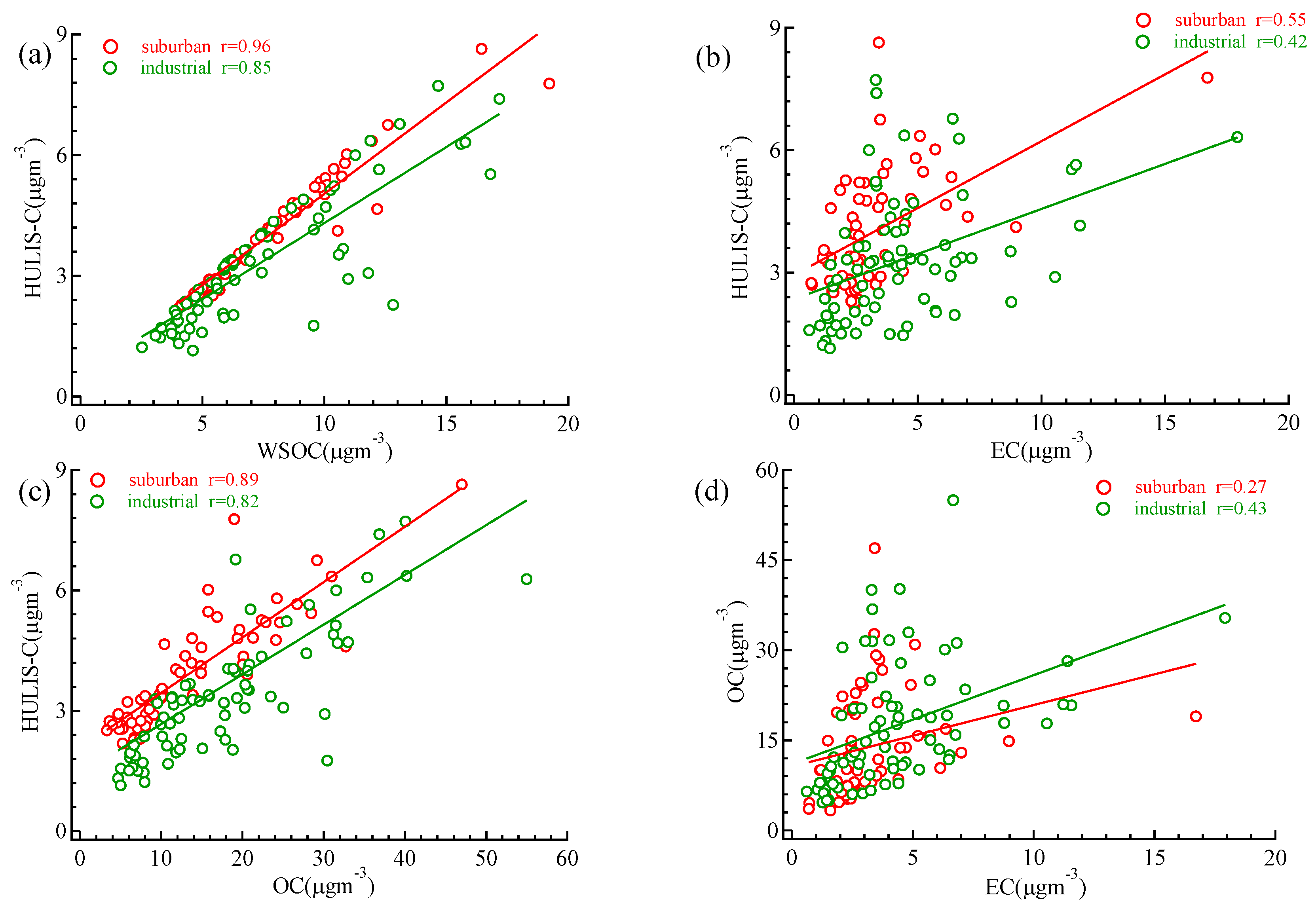
3.4. Correlation between HULIS-C and Chemical Species

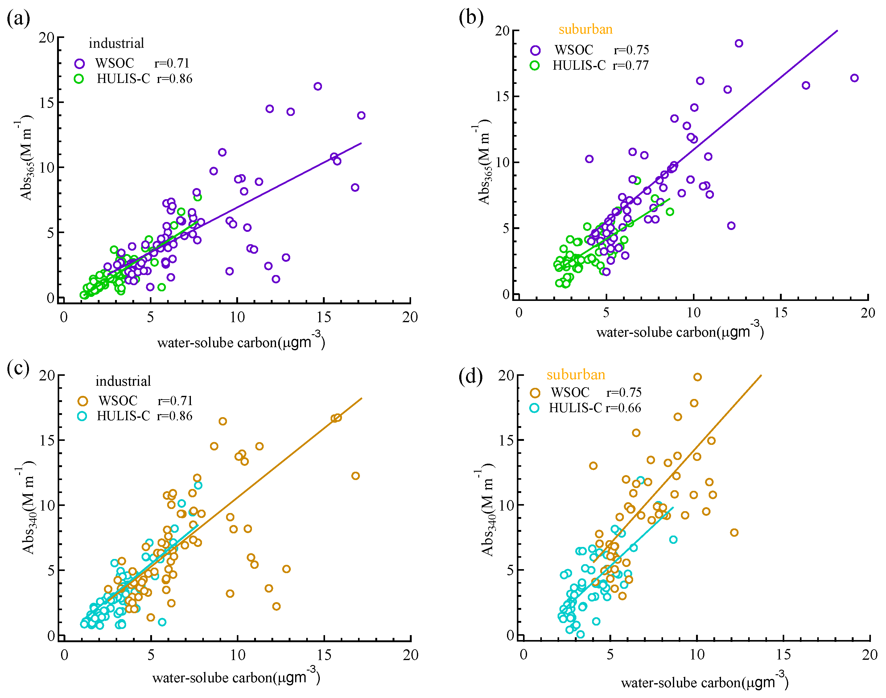
3.4.1. Interplay between HULIS-C and Carbonaceous Components

Figure 5a–c show the correlation scatter plots of HULIS-C vs. carbonaceous components (WSOC, OC, and EC) at the two sites. Moreover, the scatter plots of OC vs. EC are also presented in Figure 5d. The observed highly positive correlations between HULIS-C, WSOC, and OC demonstrated that three species share common sources. Further, we attempted to find the correlation between HULIS-C and primary emissions, such as EC (mainly produced from combustion sources and as a representative primary emission indicator). As presented in Figure 5c, the correlation between HULIS-C and EC was weak, especially in the industrial region, indicating that EC was actually not an influential source of HULIS-C, implying vehicle emissions were not the main source of HULIS. A weak correlation between OC and EC showed their distinct sources. According to Table 1, in our study, the mean OC/EC ratio was about 5.0 (4.87 in the industrial region and 4.97 in the suburban region). The average OC/EC ratio was significantly higher on polluted days (6.28) than on fair days (3.57) at the suburban site. Conversely, no distinct difference was found in the industrial region (O/C = 4.47 on fair and 5.06 on polluted days), which might be explained by high primary emissions such as PAHs and EC [43] and relatively small contributions from secondary sources on polluted days.

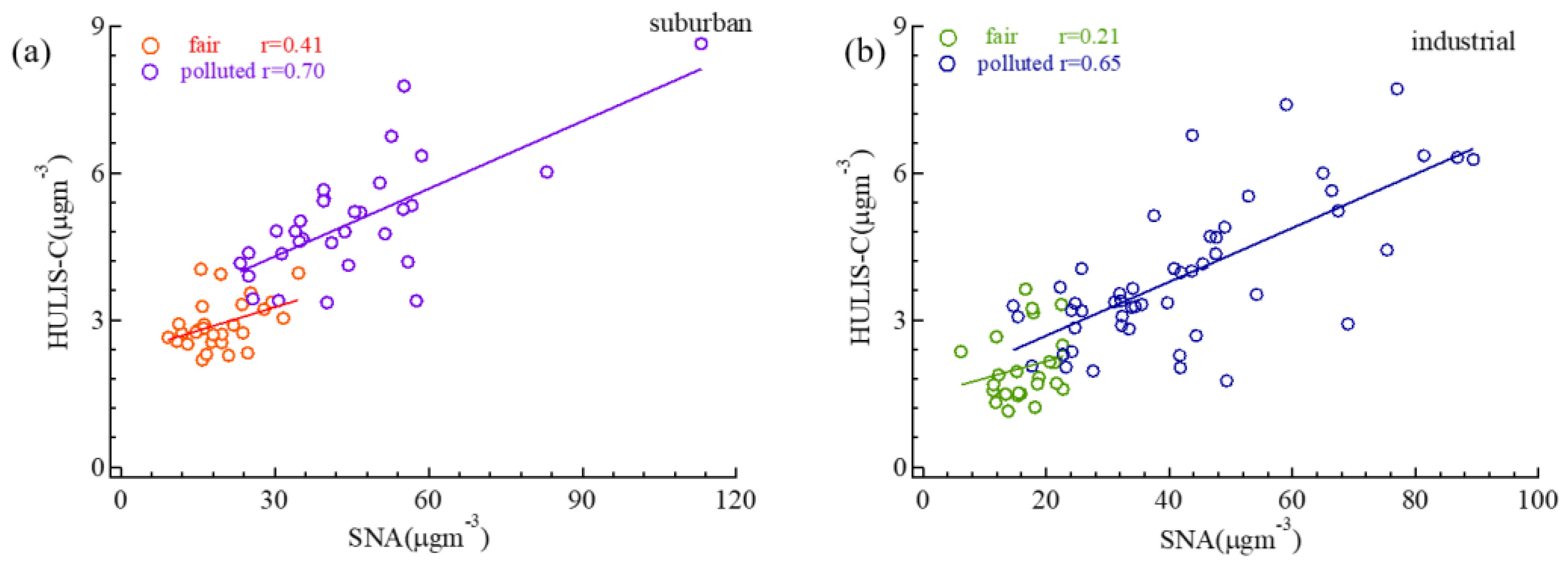
3.4.2. Relationship between HULIS-C and SNA

From Figure 6, significant correlations were also observed between HULIS-C and secondary inorganic ions at the two sites. Figure S4 depicts the scatterplot of HULIS-C with SO₄²⁻, NO₃⁻, and NH₄⁺ at both sites. As presented in Figure 6 and Figure S4, correlation coefficients between HULIS-C and SNA were generally higher on polluted days than on fair days regardless of sampling sites, implying more secondary formation on polluted days. A previous study [44] showed BB and secondary formation processes were two main sources for HULIS in winter. In Figure S4, a relatively weaker correlation between HULIS-C and sulfate than between HULIS-C and NO₃⁻ possibly indicated that coal combustion was not an important source of HULIS.

3.4.3. Relationship between HULIS-C and Some Specific Tracers

Table 3. Correlation coefficients (r) of HULIS-C with some specific tracers, including K_b, AMS ions, formate, and oxalate in the industrial region.

Species	HULIS-C	Formate	Oxalate	Kb	C2H4O2+	C3H5O2+	C4H9+	C4H7+	CO2+	C2H4O+
HULIS-C	1
formate	0.856	1
oxalate	0.481	0.426	1
Kb	0.817	0.744	0.396	1
C2H4O2+	0.736	0.737	0.303	0.711	1
C3H5O2+	0.710	0.738	0.339	0.658	0.982	1
C4H9+	0.699	0.626	0.374	0.597	0.897	0.920	1
C4H7+	0.718	0.693	0.397	0.605	0.914	0.949	0.978	1
CO2+	0.533	0.680	0.053	0.470	0.816	0.849	0.716	0.783	1
C2H4O+	0.509	0.329	0.483	0.465	0.640	0.614	0.691	0.637	0.170	1

and

Table 4. Correlation coefficients (r) of HULIS-C with some specific tracers, including K⁺, AMS ions, formate, and oxalate in the suburban region.

Species	HULIS-C	Formate	Oxalate	Kb	C2H4O2+	C3H5O2+	C4H9+	C4H7+	CO2+	C2H4O+
HULIS-C	1
formate	−0.054	1
oxalate	0.026	0.824	1
Kb	0.289	0.031	−0.077	1
C2H4O2+	0.253	0.403	0.013	0.315	1
C3H5O2+	0.435	0.198	0.069	0.342	0.782	1
C4H9+	0.652	0.063	0.010	0.317	0.662	0.934	1
C4H7+	0.660	0.078	0.044	0.274	0.624	0.949	0.973	1
CO2+	0.489	0.258	0.051	0.449	0.878	0.947	0.874	0.861	1
C2H4O+	0.312	0.298	0.010	0.243	0.937	0.812	0.719	0.695	0.849	1

summarize the correlation coefficients of HULIS-C with some specific tracers, including K⁺, AMS tracer ions, formate, and oxalate. A strong correlation between HULIS-C with corrected K⁺ (r = 0.817) indicated that BB was a significant source of HULIS-C in the industrial region. This was further supported by the correlations between HULIS-C and AMS BB tracers such as C₂H₄O₂⁺ (r = 0.736) and C₃H₅O₂⁺ (r = 0.710) ions detected by SP–AMS. This finding was similar to our previous studies [28,45]. In contrast, relatively weak correlations between HULIS-C with K_b (r = 0.289), C₃H₅O₂⁺ (r = 0.435), and C₂H₄O₂⁺ (r = 0.253) were observed in the suburban area, suggesting the limited contribution of BB to winter HULIS. We found moderate/tight correlations between HULIS-C with oxalate (0.481) and formate (r = 0.856) in the industrial region, suggesting secondary reactions could be a possible source of HULIS-C. Consistently, previous studies have also shown the formation pathways of HULIS and oxalate are similar, i.e., heterogeneous process, and/or photochemical oxidation, and biomass burning sources [46,47,48]. On the other hand, HULIS-C and oxalate (r = 0.026) and formate (−0.054) in the suburban area showed no correlations.

In summary, the poor correlation of HULIS-C with EC, together with the tight correlation with SNA and moderate relation with K_b, indicates that that secondary reaction and BB are two major sources of HULIS-C during winter.

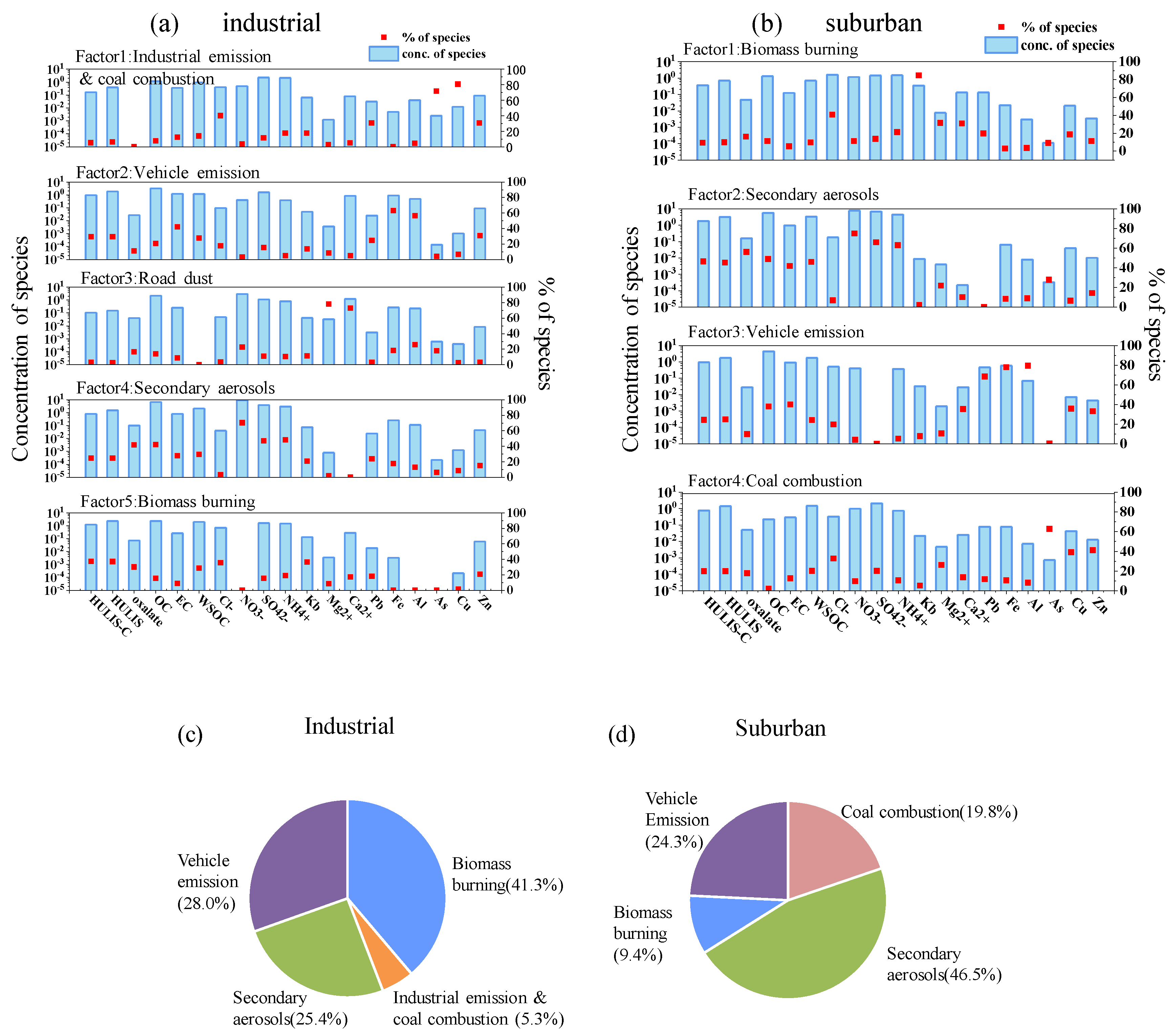
3.5. PMF Analysis for Potential Sources of HULIS

The PMF-apportioned source contributions to HULIS and HULIS-C at both sites are shown in Figure 7. A strong linear correlation between the measured and PMF-reconstructed HULIS mass concentrations (suburban: r = 0.92; industrial: r = 0.97) demonstrates the validity and robustness of our PMF solutions (Figure S5 in the Supplement).

As shown in Figure 7a in the industrial region, Factor 1 was dominated by As, Cu, Zn, Pb, and Cl⁻, so it was treated as being from industrial emissions and coal combustion. Factor 2 was characterized by high percentages of Fe, Al, and Zn, and EC also contributed to some extent; thus, it was considered as a vehicle emission source [49]. Factor 3 was considered to be road dust due to the high loadings of Mg²⁺ and Ca²⁺ in its profile. The main components of Factor 4 were SNA (SO₄²⁻, NO₃⁻ and NH₄⁺) and oxalate, and it was therefore designated as secondary aerosols. Factor 5 contained a high proportion of K_b, moderate Cl^-, and very low As; thus, it was determined as a biomass burning source [50]. Among the five identified sources, factor 5 contributed the most to HULIS-C. It was worthy to note that road dust contribution to HULIS-C was very low, so we ignored this factor in further discussion. The PMF model was also used to determine the possible sources of HULIS in the suburban region. Similarly, as shown in Figure 7b, Factor 1 and Factor 2 were considered as biomass burning and secondary aerosols sources, respectively. Factor 3 was dominated by Zn, Pb, Fe, Al, and EC and was designated to be vehicle emissions. Factor 4 was characterized by a predominant loading of As, Zn, and Cu and was viewed as a coal combustion source. The contribution of factor 2 ranked first among all identified sources for HULIS in the suburban region. In this study, the sampling site of the suburban area was located near Zhongwu Road, influenced by considerable vehicular emissions such as NOx, which may have led to subsequent significant secondary formation.

Based on PMF results, we also calculated the source-specific contributions to HULIS-C mass concentration at these two sites (Figure 7c,d). Biomass burning was the largest contributor (41.3%) to HULIS-C in the industrial region. Vehicle emissions were the second largest (28.0%) contributor to HULIS-C, followed by secondary aerosols, which accounted for 25.4%. In contrast, secondary aerosols were the most significant contributor to HULIS-C (46.5%) in the suburban region, with the three primary sources, i.e., biomass burning, vehicle emissions, and coal combustion, accounting for 53.5% in total.

In summary, despite some differences in the contributions to the HULIS-C mass at the two sites, biomass burning, secondary aerosols and vehicle emissions were found to be three common sources of HULIS-C, and they accounted for 41.3%, 25.4%, and 28.0% in the industrial region, and 9.4%, 46.5%, and 24.3%, respectively, in the suburban region. HULIS-C in the industrial region was relatively strongly affected by the biomass burning, and the primary pollution in the industrial region was serious. In contrast, secondary processes seemed to be more important to HULIS-C in the suburban region than in the industrial region.

4. Conclusions

Water-soluble HULIS-C accounted for 21.1% of OC in the industrial region and 35.1% of OC in the suburban region, illustrating the important role of HULIS in atmospheric aerosols. The HULIS and WSOC fractions in PM_2.5 were lower in the industrial area than in the suburban area due to the combined impacts of different HULIS sources at these two sites. During polluted days, HULIS values were in the range of 3.67–15.32 and 6.09–16.21 µg m⁻³ in the industrial and suburban region, respectively, compared with 2.26–6.54 and 3.96–7.55 µg m⁻³ during fair days. The high OC/EC ratios indicated the importance of secondary formation processes throughout the sampling period. The much higher SNA contribution to PM_2.5 on polluted days further supports the importance of secondary processes of inorganic species in haze. The wavelength dependence of MAE₃₆₅ of HULIS-C was different under three different PM_2.5 levels, with the highest MAE₃₆₅ value on severely polluted days, suggesting HULIS could contribute significantly to haze formation due to their strong light absorbing property.

PM_2.5 HULIS from the industrial site exhibited slightly higher MAE₂₈₀, MAE₃₆₅, and AAE_300–400 values. In comparison to fair days, high MAE₂₈₀ and MAE₃₆₅ values for HULIS fractions were also found on polluted days, indicating the presence of abundant compounds with high aromaticity or different emission/secondary formations. No clear differences in AAE_300–400 and E₂/E₃ values for HULIS and the original WSOC were observed at the two sites, indicating HULIS were the major components of WSOC.

Good correlations of PM_2.5 HULIS-C with both BB tracers (i.e., K_b, C₂H₄O₂⁺, C₃H₅O₂⁺) and SNA suggested BB emissions and secondary formation processes were the two major sources of HULIS in the industrial region, especially on polluted days. On the contrary, relative weak correlations between HULIS-C with the aforementioned BB tracers implied the limited contribution of biomass burning to suburban HULIS-C. Three primary sources (i.e., biomass burning, industrial emission/coal combustion, and vehicle emissions) and one secondary source were identified by PMF in the industrial region. Moreover, four sources, i.e., biomass burning, vehicle emissions, coal combustion, and secondary aerosols, were identified by PMF in the suburban region. Secondary sources were the major contributor to HULIS-C, followed by vehicle emissions, coal combustion, and biomass burning in the suburban area. The contributions of primary sources to HULIS overall outweighed those of secondary sources throughout the episode at both sites (industrial: 74.6%, suburban: 53.5%).

Our findings relate to PM_2.5 chemistry and its future reductions. Further investigations on other properties of PM_2.5 HULIS in these two sites are yet to be conducted, including ROS generation and molecular characterization of HULIS, in order better address the possible health effects of HULIS.

References

1. Baduel, C.; Voisin, D.; Jaffrezo, J.L. Comparison of analytical methods for humic like substances (HULIS) measurements in atmospheric particles. Atmos. Chem. Phys. 2009, 9, 5949–5962. [Google Scholar] [CrossRef] [Green Version]
2. Hoffer, A.; Gelencsér, A. Optical properties of humic-like substances (HULIS) in. Atmos. Chem. Phys. 2006, 6, 3563–3570. [Google Scholar] [CrossRef] [Green Version]
3. Yu, S.; Liu, W.; Xu, Y.; Yi, K.; Zhou, M.; Tao, S.; Liu, W. Characteristics and oxidative potential of atmospheric PM2.5 in Beijing: Source apportionment and seasonal variation. Sci. Total. Environ. 2019, 650, 277–287. [Google Scholar] [CrossRef]
4. Win, M.; Tian, Z.; Zhao, H.; Xiao, K.; Peng, J.; Shang, Y.; Wu, M.; Xiu, G.; Lu, S.; Yonemochi, S.; et al. Atmospheric HULIS and its ability to mediate the reactive oxygen species (ROS): A review. J. Environ. Sci. 2018, 71, 13–31. [Google Scholar] [CrossRef] [PubMed]
5. Lu, S.; Win, M.; Zeng, J.; Yao, C.; Zhao, M.; Xiu, G.; Lin, Y.; Xie, T.; Dai, Y.; Rao, L.; et al. A characterization of HULIS-C and the oxidative potential of HULIS and HULIS-Fe(II) mixture in PM2.5 during hazy and non-hazy days in Shanghai. Atmos. Environ. 2019, 219, 117058. [Google Scholar] [CrossRef]
6. Xu, X.; Lu, X.; Li, X.; Liu, Y.; Wang, X.; Chen, H.; Chen, J.; Yang, X.; Fu, T.; Zhao, Q.; et al. ROS-generation potential of Humic-like substances (HULIS) in ambient PM2.5 in urban Shanghai: Association with HULIS concentration and light absorbance. Chemosphere 2020, 256, 127050. [Google Scholar] [CrossRef]
7. Ma, Y.; Cheng, Y.; Qiu, X.; Cao, G.; Kuang, B.; Yu, J.; Hu, D. Optical properties, source apportionment and redox activity of humic-like substances (HULIS) in airborne fine particulates in Hong Kong. Environ. Pollut. 2019, 255, 113087. [Google Scholar] [CrossRef]
8. Chen, Q.; Ikemori, F.; Higo, H.; Asakawa, D.; Mochida, M. Chemical structural characteristics of HULIS and other fractionated organic matter in urban aerosols: Results from mass spectral and FT-IR analysis. Environ. Sci. Technol. 2016, 50, 1721–1730. [Google Scholar] [CrossRef] [PubMed]
9. Ma, Y.; Cheng, Y.; Gao, G.; Yu, J.; Hu, D. Speciation of carboxylic components in humic-like substances (HULIS) and source apportionment of HULIS in ambient fine aerosols (PM2.5) collected in Hong Kong. Environ. Sci. Pollut. Res. 2020, 27, 23172–23180. [Google Scholar] [CrossRef]
10. Tan, J.; Xiang, P.; Zhou, X.; Duan, J.; Ma, Y.; He, K.; Cheng, Y.; Yu, J.; Querol, X. Chemical characterization of humic-like substances (HULIS) in PM2.5 in Lanzhou, China. Sci. Total. Environ. 2016, 573, 1481–1490. [Google Scholar] [CrossRef]
11. Tang, S.; Li, F.; Tsona, N.; Lu, C.; Wang, X.; Du, L. Aqueous-phase photooxidation of vanillic acid: A potential source of humic-like substances (HULIS). ACS Earth Space Chem. 2020, 4, 862–872. [Google Scholar] [CrossRef]
12. Ye, Z.; Qu, Z.; Ma, S.; Luo, S.; Chen, Y.; Chen, H.; Chen, Y.; Zhao, Z.; Chen, M.; Ge, X. A comprehensive investigation of aqueous-phase photochemical oxidation of 4-ethylphenol. Sci. Total. Environ. 2019, 685, 976–985. [Google Scholar] [CrossRef] [PubMed]
13. Lee, J.Y.; Jung, C.H.; Kim, Y.P. Estimation of optical properties for HULIS aerosols at anmyeon Island, Korea. Atmosphere 2017, 8, 120. [Google Scholar] [CrossRef] [Green Version]
14. Kristensen, T.B.; Du, L.; Nguyen, Q.T.; Nøjgaard, J.K.; Koch, C.B.; Nielsen, O.F.; Hallar, A.G.; Lowenthal, D.H.; Nekat, B.; Pinxteren, D.; et al. Chemical properties of HULIS from three different environments. J. Atmos. Chem. 2015, 72, 65–80. [Google Scholar] [CrossRef]
15. Liu, B.; Li, Y.; Wang, L.; Bi, X.; Dong, H.; Sun, X.; Xiao, Z.; Zhang, Y.; Feng, Y. Source directional apportionment of ambient PM2.5 in urban and industrial sites at a megacity in China. Atmos. Res. 2020, 235, 104764. [Google Scholar] [CrossRef]
16. Yu, Y.; Yao, S.; Dong, H.; Wang, L.; Wang, C.; Ji, X.; Ji, M.; Yao, X.; Zhang, Z. Association between short-term exposure to particulate matter air pollution and cause-specific mortality in Changzhou, China. Environ. Res. 2019, 170, 7–15. [Google Scholar] [CrossRef]
17. Liu, B.; Wu, J.; Zhang, J.; Wang, L.; Yang, J.; Liang, D.; Dai, Q.; Bi, X.; Feng, Y.; Zhang, Y.; et al. Wintertime aerosol chemistry and haze evolution in an extremely polluted city of the North China Plain: Significant contribution from coal and biomass combustion. Atmos. Chem. Phys. 2017, 17, 4751–4768. [Google Scholar] [CrossRef] [Green Version]
18. Ye, Z.; Li, Q.; Ma, S.; Zhou, Q.; Gu, Y.; Su, Y.; Chen, Y.; Chen, H.; Wang, J.; Ge, X. Summertime day-night differences of PM2.5 components (inorganic ions, OC, EC, WSOC, WSON, HULIS, and PAHs) in Changzhou, China. Atmosphere 2017, 8, 189. [Google Scholar] [CrossRef] [Green Version]
19. Ye, Z.; Liu, J.; Gu, A.; Feng, F.; Liu, Y.; Bi, C.; Xu, J.; Li, L.; Chen, H.; Chen, Y. Chemical characterization of fine particulate matter in Changzhou, China, and source apportionment with offline aerosol mass spectrometry. Atmos. Chem. Phys. 2017, 17, 2573–2592. [Google Scholar] [CrossRef] [Green Version]
20. Qi, L.; Zhang, Y.; Ma, Y.; Chen, M.; Ge, X.; Ma, Y.; Zheng, J.; Wang, Z.; Li, S. Source identification of trace elements in the atmosphere during the second Asian Youth Games in Nanjing, China: Influence of control measures on air quality. Atmos. Pollut. Res. 2016, 7, 547–556. [Google Scholar] [CrossRef]
21. Bi, C.; Chen, Y.; Zhao, Z.; Li, Q.; Zhou, Q.; Ye, Z.; Ge, X. Characteristics, sources and health risks of toxic species (PCDD/Fs, PAHs and heavy metals) in PM2.5 during fall and winter in an industrial area. Chemosphere 2020, 238, 124620. [Google Scholar] [CrossRef]
22. Onasch, T.B.; Trimborn, A.; Fortner, E.C.; Jayne, J.T.; Kok, G.L.; Williams, L.R.; Davidovits, P.; Worsnop, D.R. Soot particle aerosol mass spectrometer: Development, validation, and initial application. Aerosol. Sci. Technol. 2012, 46, 804–817. [Google Scholar] [CrossRef]
23. Wang, J.; Zhang, Q.; Chen, M.; Collier, S.; Zhou, S.; Ge, X.; Xu, J.; Shi, J.; Xie, C.; Hu, J.; et al. First chemicalcharacterization of refractory black carbon aerosols and associated coatings over the Tibetan Plateau (4730 m a.s.l). Environ. Sci. Technol. 2017, 51, 14072–14082. [Google Scholar] [CrossRef]
24. Wang, J.; Ge, X.; Chen, Y.; Shen, Y.; Zhang, Q.; Sun, Y.; Xu, J.; Ge, S.; Yu, H.; Chen, M. Highly time-resolved urban aerosol characteristics during springtime in Yangtze River Delta, China: Insights from soot particle aerosol mass spectrometry. Atmos. Chem. Phys. 2016, 16, 9109–9127. [Google Scholar] [CrossRef] [Green Version]
25. Ge, X.; Li, L.; Chen, Y.; Chen, H.; Wu, D.; Wang, J.; Xie, X.; Ge, S.; Ye, Z.; Xu, J.; et al. Aerosol characteristics and sources in Yangzhou, China resolved by offline aerosol mass spectrometry and other techniques. Environ. Pollut. 2017, 225, 74–85. [Google Scholar] [CrossRef] [PubMed]
26. Ye, Z.; Li, Q.; Liu, J.; Luo, S.; Zhou, Q.; Bi, C.; Ma, S.; Chen, Y.; Chen, H.; Li, L.; et al. Investigation of submicron aerosol characteristics in Changzhou, China: Composition, source, and comparison with co-collected PM2.5. Chemosphere 2017, 183, 176–185. [Google Scholar] [CrossRef]
27. Shen, Z.; Zhang, Q.; Cao, J.; Zhang, L.; Lei, Y.; Huang, Y.; Huang, R.J.; Gao, J.; Zhao, Z.; Zhu, C.; et al. Optical properties and possible sources of brown carbon in PM2.5 over Xi’an, China. Atmos. Environ. 2017, 150, 322–330. [Google Scholar] [CrossRef]
28. Chen, Y.; Ge, X.; Chen, H.; Xie, X.; Chen, Y.; Wang, J.; Ye, Z.; Bao, M.; Zhang, Y.; Chen, M. Seasonal light absorption properties of water-soluble brown carbon in atmospheric fine particles in Nanjing, China. Atmos. Environ. 2018, 187, 230–240. [Google Scholar] [CrossRef]
29. Wu, G.; Wan, X.; Gao, S.; Fu, P.; Yin, Y.; Li, G.; Zhang, G.; Kang, S.; Ram, K.; Cong, Z. Humic-like substances (HULIS) in aerosols of Central Tibetan Plateau (Nam Co, 4730 m asl): Abundance, light absorption properties, and sources. Environ. Sci. Technol. 2018, 52, 7203–7211. [Google Scholar] [CrossRef]
30. Zhang, X.; Lin, Y.; Surratt, J.; Weber, R. Sources, Composition and Absorption Ångström Exponent of light-absorbing organic components in aerosol Extracts from the Los Angeles Basin. Environ. Sci. Technol. 2013, 47, 3685–3693. [Google Scholar] [CrossRef] [PubMed]
31. Huo, Y.; Li, M.; Jiang, M.; Qi, W. Light absorption properties of HULIS in primary particulate matter produced by crop straw combustion under different moisture contents and stacking modes. Atmos. Environ. 2018, 191, 490–499. [Google Scholar] [CrossRef]
32. Ma, Y.; Cheng, Y.; Qiu, X.; Cao, G.; Fang, Y.; Wang, J.; Zhu, T.; Yu, J.; Hu, D. Sources and oxidative potential of water-soluble humic-like substances (HULISWS) in fine particulate matter (PM2.5) in Beijing. Atmos. Chem. Phys. 2018, 18, 5607–5617. [Google Scholar] [CrossRef] [Green Version]
33. Yu, J.; Yan, C.; Liu, Y.; Li, X.; Zhou, T.; Zheng, M. Potassium: A tracer for biomass burning in Beijing? Aerosol Air Qual. Res. 2017, 18, 2447–2459. [Google Scholar] [CrossRef] [Green Version]
34. Pachon, J.E.; Weber, R.J.; Zhang, X.L.; Mulholland, J.A.; Russell, A.G. Revising the use of potassium (K) in the source apportionment of PM2.5. Atmos. Pollut. Res. 2013, 4, 14–21. [Google Scholar] [CrossRef] [Green Version]
35. Zhao, M.; Qiao, T.; Li, Y.; Tang, X.; Xiu, G.; Yu, J. Temporal variations and source apportionment of Hulis-C in PM2.5 in urban Shanghai. Sci. Total. Environ. 2016, 571, 18–26. [Google Scholar] [CrossRef]
36. Fan, X.; Song, J.; Peng, P. Temporal variations of the abundance and optical properties of water soluble Humic-like substances (HULIS) in PM2.5 at Guangzhou, China. Atmos. Res. 2016, 172–173, 8–15. [Google Scholar] [CrossRef]
37. Zhang, T.; Shen, Z.; Zhang, L.; Tang, Z.; Zhang, Q.; Chen, Q.; Lei, Y.; Zeng, Y.; Xu, H.; Cao, J. PM2.5 Humic-like substances over Xi’an, China: Optical properties, chemical functional group, and source identification. Atmos. Res. 2020, 234, 104784. [Google Scholar] [CrossRef]
38. Lin, P.; Huang, X.; He, L.; Zhen, Y. Abundance and size distribution of HULIS in ambient aerosols at a rural site in South China. J. Aerosol Sci. 2010, 41, 74–87. [Google Scholar] [CrossRef]
39. Baduel, C.; Voisin, D.; Jaffrezo, J.L. Seasonal variations of concentrations and optical properties of water soluble HULIS collected in urban environments. Atmos. Chem. Phys. 2010, 10, 4085–4095. [Google Scholar] [CrossRef] [Green Version]
40. Zhang, Y.; Huang, W.; Cai, T.; Fang, D.; Wang, Y.; Song, J.; Hu, M.; Zhang, Y. Concentrations and chemical compositions of fine particles (PM2.5) during haze and non-haze days in Beijing. Atmos. Res. 2016, 174–175, 62–69. [Google Scholar] [CrossRef]
41. Fan, X.; Li, M.; Cao, T.; Cheng, C.; Li, F.; Xie, Y.; Wei, S.; Song, J.; Peng, P. Optical properties and oxidative potential of water-and alkaline-soluble brown carbon in smoke particles emitted from laboratory simulated biomass burning. Atmos. Environ. 2018, 194, 48–57. [Google Scholar] [CrossRef]
42. Zou, C.; Li, M.; Cao, T.; Zhu, M.; Fan, X.; Peng, S.; Song, J.; Jiang, B.; Jia, W.; Yu, C.; et al. Comparison of solid phase extraction methods for the measurement of humic-like substances (HULIS) in atmospheric particles. Atmos. Environ. 2020, 225, 117370. [Google Scholar] [CrossRef]
43. Huang, R.; Yang, L.; Cao, J.; Chen, Y.; Chen, Q.; Li, Y.; Duan, J.; Zhu, C.; Dai, W.; Wang, K.; et al. Brown carbon aerosol in urban Xi’an, Northwest China: The composition and light absorption properties. Environ. Sci. Technol. 2018, 52, 6825–6833. [Google Scholar] [CrossRef]
44. Qiao, T.; Zhao, M.; Xiu, G.; Yu, J. Seasonal variations of water soluble composition (WSOC, Hulis and WSIIs) in PM1 and its implications on haze pollution in urban Shanghai, China. Atmos. Environ. 2015, 123, 306–314. [Google Scholar] [CrossRef]
45. Chen, Y.; Xie, X.; Shi, Z.; Li, Y.; Gai, X.; Wang, J.; Li, H.; Wu, Y.; Zhao, X.; Chen, M.; et al. Brown carbon in atmospheric fine particles in Yangzhou, China: Light absorption properties and source apportionment. Atmos. Res. 2020, 244, 105028. [Google Scholar] [CrossRef]
46. Win, M.; Zeng, J.; Yao, C.; Zhao, M.; Xiu, G.; Xie, T.; Rao, L.; Zhang, L.; Lu, H.; Liu, X.; et al. Sources of HULIS-C and its relationships with trace metals, ionic species in PM2.5 in suburban Shanghai during haze and non-haze days. J. Aerosol. Sci. 2020, 77, 63–81. [Google Scholar] [CrossRef]
47. Zhou, X.; Zhang, L.; Tan, J.; Zhang, K.; Mao, J.; Duan, J.; Hu, J. Characterization of humic-like substances in PM2.5 during biomass burning episodes on Weizhou Island, China. Atmos. Environ. 2018, 191, 258–266. [Google Scholar] [CrossRef]
48. Park, S.; Son, S.; Lee, S. Characterization, sources, and light absorption of fine organic aerosols during summer and winter at an urban site. Atmos. Res. 2018, 213, 370–380. [Google Scholar] [CrossRef]
49. Yin, X.; Fan, G.; Liu, J.; Jiang, T.; Wang, L. Characteristics of heavy metals and persistent organic pollutants in PM2.5 in two typical industrial cities, North China. Environ. Forensics 2020, 21, 250–258. [Google Scholar] [CrossRef]
50. Li, X.; Yang, K.; Han, J.; Ying, Q.; Hopke, P.K. Sources of humic-like substances (HULIS) in PM2.5 in Beijing: Receptor modeling approach. Sci. Total Environ. 2019, 671, 765–775. [Google Scholar] [CrossRef]
Figure 1. Temporal variation of PM2.5 and its constituents (i.e., HULIS-C, HULIS, OC, EC, WSOC, SNA, oxalate, and formate), as well as optical properties (E2/E3, MAE280, MAE365) of HULIS at the two sites. (a) suburban region, (b) industrial region.
Atmosphere 12 00276 g001
Figure 2. Wavelength dependences of the light absorption coefficient (Abs) (a) and mass ab-sorption efficiency (MAE) (b) for water-soluble organic carbon (WSOC), as well as Abs of the humic-like substance (HULIS) (c) and MAE of HULIS (d) in the industrial region.
Atmosphere 12 00276 g002
Figure 3. Scatter plots of Abs365 versus HULIS-C and WSOC at the two sites (a,b) and Abs340 versus HULIS-C and WSOC (c,d).
Atmosphere 12 00276 g003
Figure 4. (a,b) Correlations between MAE280 and HULIS-C, (c,d) variation of E2/E3 with HULIS-C concentration at the two sites.
Atmosphere 12 00276 g004
Figure 5. The scatter plots of HULIS-C versus carbonaceous components. (a)WSOC, (b) OC, and (c) EC at the two sites. (d) Correlations between OC and EC.
Atmosphere 12 00276 g005
Figure 6. Correlations between HULIS-C concentration and secondary inorganic ion (SNA = NH4+ + NO3 + SO42−) concentration in industrial (a), and suburban (b) regions.
Atmosphere 12 00276 g006
Figure 7. (a,b). Distribution of HULIS, HULIS-C mass, and chemical species associated with four factors resolved by PMF at the two sampling site (left axis, blue bars: mass concentration of each species apportioned to the factor) and explained variance (right axis, red spots) of each species apportioned to the factor). (c,d). contributions of PMF factors to HULIS-C mass.
Atmosphere 12 00276 g007