Article

Baltic Sea Spray Emissions: In Situ Eddy Covariance Fluxes vs. Simulated Tank Sea Spray

by
Ernst Douglas Nilsson
1,2,*,
Kim A. H. Hultin
1,
Eva Monica Mårtensson
3,
Piotr Markuszewski
1,2,4,
Kai Rosman
1 and
Radovan Krejci
1,2
1
Department of Environmental Science, Stockholm University, 10691 Stockholm, Sweden
2
Bolin Centre for Climate Research, Stockholm University, 10691 Stockholm, Sweden
3
Department of Earth Sciences, Uppsala University, 75236 Uppsala, Sweden
4
Physical Oceanography Department, Institute of Oceanology, Polish Academy of Sciences, 81-712 Sopot, Poland
*
Author to whom correspondence should be addressed.
Atmosphere 2021, 12(2), 274; https://doi.org/10.3390/atmos12020274
Submission received: 24 December 2020 / Revised: 10 February 2021 / Accepted: 13 February 2021 / Published: 18 February 2021

Abstract

:
We present the first ever evaluation of sea spray aerosol eddy covariance (EC) fluxes at near coastal conditions and with limited fetch, and the first over water with brackish water (on average 7 ppt). The measurements were made on the island of Garpen in the Baltic Sea (56°23′ N, 16°06′ E) in September 2005. We found that wind speed is a major factor that is driving an exponential increase in sea spray sea salt emissions, comparable to previous studies over waters with higher salinity. We were able to show that the inclusion of a thermodenuder in the EC system allowed for the parallel measurements of the dry unheated aerosol flux (representing both organic and sea salt sea spray emissions) and the heated (300 °C) non-volatile sea salt emissions. This study’s experimental approach also included measurements of the artificial sea spray formed in a tank in locally sampled water at the same location as the EC fluxes. We attempted to use the EC aerosol flux measurements to scale the tank measurements to aerosol emissions in order to derive a complete size distribution for the sea spray emission fluxes below the size range (0.3–2 µm dry diameter) of the optical particle counters (OPCs) in the EC system, covering in total 0.01 µm to 2 µm diameter. In the wind directions with long fetches (corresponding to conditions similar to open sea), we were able to distinguish between the aerosol emission fluxes of dry aerosol and heated non-volatile (sea salt only) in the smallest size bins of the OPC, and could therefore indirectly estimate the organic sea spray fraction. In agreement with several previous ambient and tank experiments deriving the size resolved chemical mass concentration of sea salt and water-insoluble organic sea spray, our EC fluxes showed that sea sprays were dominated by sea salt at sizes ≥1 µm diameter, and by organics at the smallest OPC sizes. Since we used direct measures of the sea spray emission fluxes, we confirmed previous suggestions that this size distribution of sea salt and organics is a signature of sea spray aerosols. We were able to show that two sea salt source parameterizations (Mårtensson et al. (2003) and Salter et al. (2015)) agreed fairly well with our observed heated EC aerosol emission fluxes, as long as their predicted emissions were modified for the actual salinity by shifting the particle diameters proportionally to the cubic rote of the salinity. If, in addition, we added organics to the parameterized sea spray following the mono-layer model by Ellison et al. (1999), the combined sea spray parameterizations for sea salt and organics fell reasonably close to the observed fluxes for diameters > 0.15 µm, while one of them overpredicted the sea spray emissions below this size. The organic mono-layer model by Ellison et al. appeared to be able to explain most of the differences we observed between the aerosol emission fluxes with and without the thermodenuder.

1. Introduction

Bubble-bursting from whitecaps, created by wind-generated waves breaking, is considered the most effective mechanism for ejecting sea spray into the atmosphere from the ocean surface [1]. According to the standard model, when a bubble reaches the ocean surface, the liquid film surrounding it drains off, resulting in a weakening of the bubble film, which thereafter ruptures, thereby producing a large number of film droplets bigger than 2 mm [2,3]. Following the rupture of the bubble film, large jet droplets would then issue from the instability and subsequent break-up of a liquid jet that shoots up from the bubble cavity [1,4]. Usually, film drops are said to account for the dry size sub-micrometer sea spray sea salt, with the super-micrometer sea spray making up the jet drops (together with spume drops) [5,6].
Above roughly 4 ms−1, the wind stress at the open ocean surface (which corresponds to 10 ms−1 wind speed) is sufficient to cause breaking waves and thus a flux of sea spray particles into the atmosphere [7]. Wind also controls dispersion and (dry) deposition of aerosol on the sea surface, leading to loss of aerosol [8,9,10]. Environmental parameters such as salinity and water temperature, as well as the accumulated organic material in the surface water have also been observed to have a strong effect on the marine aerosol production [6,11,12,13,14,15,16,17]. Recent discoveries indicate that the standard model is, if not incorrect, at least incomplete. For example, high-speed camera studies have demonstrated the existence of daughter bubbles that form around the ruptured original bubble [18,19,20]. Surface water tension, viscosity, and density, as well as bubble properties, have been identified as key factors that separate the regime of daughter bubbles from the regimes without daughter bubbles or daughter bubbles with each other. High speed photography also shows that jet drops ejected from these daughter bubbles could contribute to the sub micrometer sea spray.
The most direct way of investigating the magnitude of aerosol net exchange between the surface and atmosphere is offered by the eddy covariance method, wherein a net upward flux indicates that particle emissions dominate over (dry deposition) sinks, as shown for marine regions [21], urban areas [22], and tropical rainforests [23]. The eddy covariance method was first applied to the measurement of sea spray fluxes by [24] over the Norwegian Sea, Barents Sea, and the Arctic Ocean. This work has been followed by studies over the northeastern Atlantic [25,26] and northwestern Atlantic [27], all of which used the eddy covariance technique at coastal sites under conditions representative of an open ocean.
While sea salt dominates the particulate mass concentration in unpolluted marine air with the global mass flux estimated to be in the vicinity of 1×10¹⁶ g y−1 [28,29], studies have however stressed that sub micrometer sea spray aerosol can hold a significant organic mass fraction as well [15,16,17,20,30,31,32,33]. Most numerous is the marine aerosol in the sub micrometer size range, sizes important for scattering effects and cloud formation [34,35], and therefore they deserve to be properly investigated. The amount of sea spray particles of all sizes emitted into the atmosphere per unit area, surface area, time, and the sea spray source function is required for modelling of the marine aerosol. Available source functions are obtained using different methods and physical principles, with most being derived from indirect methods such as the whitecap method. In the whitecap method, parameterizations of the fraction whitecap cover from field experimental data are combined with laboratory measurements of sea spray production rates per area whitecap (e.g., [6,36,37]). In particular, in order to improve climate models, accurate parameterizations of all aerosol emissions over all particle sizes are required. These include sub micrometer sea spray particles, which current models are now attempting to simulate [15,16,17,38,39,40].
The study of [25] represents the first pseudo-size-segregated (size between 10 nm and 1000 nm) aerosol flux measurements where 50% of the number flux was found in 10–100 nm and 50% in 100–500 nm diameter. To date, no established technique has been designed to measure size-segregated atmospheric fluxes with the eddy covariance method below ≈0.1 µm in size due to the slow response times of the instruments available. An REA (relaxed eddy accumulation) system could potentially allow for the use of slow aerosol sizing instrumentation [41], but is yet to be tested in marine environments, and REA is not likely to ever work aboard a moving platform such as a ship. The hope may also come from new types of instrumentation that both offer a wider size range and faster measurements, such as electric low-pressure impactors.
In the current study, we differentiate between non-volatile and volatile sea spray aerosol. In order to cover the sub-OPC (optical particle counter) size range, we attempt to connect the sea spray fluxes to simultaneous laboratory-measured sea spray. This marks the first attempt of its kind to apply this approach, as well as being the first dataset of sea spray emissions from brackish water, in highly polluted air and water, and of short fetch near coastal sea spray emissions.

2. Experimental Site and Methods
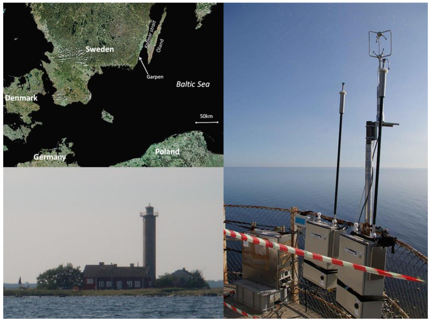
2.1. Site

Measurements were made on the Swedish southeast coast over the Baltic Sea, a polluted sea due to agriculture, eutrophication, industrial sewage, and traffic, and made worse due to the high residence time of seawater because the only connection to the open ocean is via Kattegat [42]. Due to riverine inflow of fresh water and relatively low evaporation, the water in the isolated Baltic Sea is brackish, having a salinity of about 7 ppt in the study.
The measurements were carried out at a lighthouse station on the island of Garpen (56°23’ N, 16°06’ E, Figure 1) in the southern mouth of the Kalmar Strait between the southeast coast of Sweden and the island of Öland. Garpen is a small island (300 × 75 m). The lighthouse is located at the center of the island and reaches up to 27 m above sea level. The flux system described below was mounted in the southeast side of the top platform in such a way that the light house construction only disturbed the air flow in the northwest (270°–360°).
Laboratory investigations of the aerosol produced by the bubble-bursting mechanism were performed during 7–28 September 2005 [14], while the flux measurements were extended to October. Here, we only use the flux measurements that were simultaneous to the tank experiments, and where biological production was maintained.

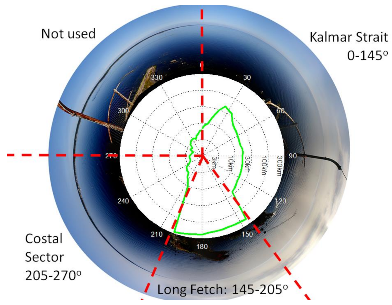
2.2. Wind Sectors, Fetch, Sea Bottom, and Footprint

Figure 2 shows the fetch from the lighthouse to the nearest coast for every compass direction. Figure 2 also includes a panorama 360° photograph stitched from 10 photographs taken at 18mm focal length. From the logarithmic fetch scale, we can identify several distinct sectors. First of all, we excluded the 270–360° sector where the flow was clearly disturbed by the lighthouse lamp housing. In the southeast 205–270° sector, we found a fetch of 2–3 km along the Swedish coastline, which can be clearly seen in the panoramic photo. In this direction, the water is shallow with depth never exceeding 6 m (see Figure 3). In the south from 145–205° towards northern Poland/Germany, we found a long fetch sector where the fetch reached about 200 to 300 km (compare Figure 1) and a water depth exceeding 10m within 1–2 km distance and 20 m within 10 km (see Figure 3), eventually reaching depths of more than 100 m. In the east, the fetch was found to be limited to about 20 km by the long, narrow island of Öland within a wide sector (0°–145°). In this direction, the depth exceeded 10 m within 1–2 km of Garpen and reached a maximum depth of about 20 m. Characteristics of the 3 sectors are summarized in Table 1. The coast of Öland was not visible for the unaided eye in most weather, and is hence not visible in the panoramic photo of Figure 2.
We used the model by [43] to estimate the footprint in the respective sectors. In the near coastal sector, where we found the highest wind speed, the maximum contribution to the fluxes originated at about 325 m from the island and 90% within 900 m at mean conditions. At most, this value varied between 400 m and 1100 m. Given the narrow size of the island of Garpen in these directions (see Figure 2) and the fetch (up to 2 km, see Figure 2 and Figure 3), this implies that the measurement footprint was dominated by water surfaces. In the long fetch sector, the largest contribution to the fluxes came from a distance of 500–800 m and 90% of the flux from within 1–2 km. In the direction of Öland, the peak flux contribution came from a distance of 300–900 m while the 90% limit never exceeded 2.5 km. This also implies that the flux was dominated by sea surface.

2.3. Weather and Air Mass Origin

Every 6 hours we calculated backward trajectories for up to 48 h, arriving at the Garpen position. Figure 4 shows those most closely associated with upward fluxes within the 3 sectors defined above: the near-coastal sector (Figure 4a), the long-fetch sector (Figure 4b), and the Kalmar Strait sector (Figure 4c). Stars denote every 12th hour. The trajectories were almost exclusively within the boundary layer. Trajectories associated with the coastal sector reached Garpen from south-westerly paths related to a strong westerly flow (and relatively high wind speed). They all passed over southern Sweden or very close to the coast prior to reaching Garpen. Before then, they originated from Denmark or Germany. Trajectories corresponding to wind from the long fetch sector were associated with a relatively slow flow from continental Europe and were due to a high pressure to the east and a low pressure to the west (Figure 4b). They did not originate from one single synoptic situation, but rather from similar conditions distributed over several occasions during the campaign. The trajectories associated with the Kalmar Strait sector spent beyond Öland several hundred kilometers over the central Baltic Sea in a counter-clockwise low-pressure circulation before originating from Sweden (Figure 4c). Despite the long distance passed over the Baltic Sea, the fetch and thereby the action of the wind on the waves were limited by the late passage of Öland.
To briefly summarize the synoptic weather during the campaign, we found that rain approached southern Sweden from the west during September 7, followed by a few days with warm but windy weather. On September 10, a high-pressure system originating from the North Sea moved up to Sweden, resulting in sunny weather (September 10–11). In the middle of September 2005, fronts originating from the remains of tropical storm Maria reached Sweden from the west. These days were characterized by low atmospheric pressure, small amounts of rain, and the highest wind speeds. This was followed by more stable weather with northerly winds shifting to westerly and then southerly with low wind speeds (September 16–22). At the end of September, a high-pressure center was located over Russia, resulting in high temperatures and southerly winds (September 26–28).

2.4. Flux Measurements

2.4.1. Instruments

A Gill ultrasonic research anemometer R3 was used to measure the 3-D wind at 20 Hz. Two Grimm Aerosol Technik GmbH 1.108 OPCs were operated together with dilution units and heaters as prototypes corresponding to the current Grimm model SVC-EDM 265. These counted the aerosol in size classes >0.3, >0.4, >0.5, >0.65, >0.8, >1.0, and >1.6 µm D with a time resolution of 1 s (this is half the number of size channels compared to when the 1.108 is operated at a lower time resolution). One system was run using a dilution unit (which diluted the sampled air with 50% dry and particle-free air) to measure the total dry aerosol. The second unit was run using a thermodenuder to heat the sampled air to 300 ℃ so as to reduce the aerosol to only the non-volatile fraction. For simplicity, we consider the aerosol below 300 ℃ as semi-volatile, and the aerosol above 300 ℃ as non-volatile. In combination with the effect of the eddy covariance method (see below) that only aerosol components with a source within the flux footprint can contribute to an upward aerosol flux, we considered the aerosol flux from the system with the thermodenuder as not only semi-volatile, but also consisting of organic compounds, since other compounds that would evaporate below 300 °C must have been transported from beyond the flux footprint. The sampling lines were 1.5 m long. The data were sampled using a lab-view flux software package developed at Stockholm University.

2.4.2. Flux Calculations

The dynamic fields of the aerosol number concentration N and vertical wind speed w can be separated into slowly varying mean fields (denoted with an overbar) and rapidly varying turbulent components (denoted with a prime): N = N ¯ + N’ and w = w ¯ + w’, respectively. In accordance with Reynold’s averaging rules, we found that the average of the product of aerosol number concentration and vertical wind speed will be the product of the average of the means plus the product of the average of the deviations: w N ¯ = w ¯ N ¯ + w N ¯ . In other words, it is the sum of the average vertical advective flux and the average vertical turbulent flux. The vertical turbulent flux of aerosol particles is the covariance between the fluctuations in aerosol concentration and in the vertical wind speed, where a positive average of w N ¯ indicates an upward flux, while a negative value indicates downward fluxes.
All eddy sizes contributing to the turbulent flux of particles should be included in the averaging time for the flux calculations, although the averaging time should be short enough to exclude long-term trends in the data. In this study, a 30-min averaging time was considered a reasonable compromise. As vertical advection was assumed to be a result of terrain, the coordinate system was rotated to obtain zero vertical advection, with the result that the total vertical flux equal to the turbulent vertical flux [44]. To remove the influence of low frequency trends in the data, we separated the fluctuations in aerosol number and vertical wind speed, N′ and w′, respectively, from the means by linear de-trending.
As noticed above, it is an important feature of eddy covariance (EC) flux measurements that upward aerosol fluxes can only result due to emissions of substances with a source in the flux footprint. Substances transported from beyond the footprint, such as sulfates, ammonia, and nitrates, would only have a minor contribution to the EC fluxes through aerosol dry deposition, and could not cause an upward flux. In combination with the thermodenuder and the dryer, we can therefore be fairly sure that upward aerosol EC flux from the system with the thermodenuder would be dominated by sea salt (plus possible small amounts of organics with even higher boiling points), while upward EC fluxes from the system with the dryer should include the same non-volatile fraction + semi-volatile organic compounds.

2.4.3. Errors and Corrections

The time lag in the aerosol sampling lines was corrected for by testing which time lag produced the largest correlation between N and w, and then using this lag to calculate the aerosol fluxes.
When data cannot be sampled as fast as the 10–20 Hz required to resolve all turbulent fluxes, or when the actual instrument’s response time is too slow, the calculated flux is underestimated. Following [45], an underestimated aerosol particle flux due to a slow response time can be estimated according to
F m F c = 1 1 + 2 π n m τ c U ¯ z α
where Fm is the measured flux and Fc the flux corrected for an underestimation due to a low response time; U is the mean horizontal wind speed; z the observation level (28 m); and τc is the frequency first order response time constant, which was 0.3 s for the OPC [23], but the logged time resolution was only 1 s. Therefore, we substituted τc with 1 s instead of 0.3 s in Equation (1). Given the short length of the sampling lines, their contribution to τc was neglected. Furthermore, α = 1 for stable stratification (z/L > 0, L is the Monin–Obukhov length that expresses a competition between mechanical and convective mixing), α = 7/8 for neutral and unstable stratifications (z/L ≤ 0), and nm is the normalized frequency:
n m = 2.0 1.915 1 + 0.5 z L ,     z / L > 0
where the limit for neutral conditions, nm = 0.085, is also applicable for unstable situations [45]. All aerosol fluxes presented in this study were corrected using Equations (1) and (2). On average, the correction was 24%.
The sampling lines were completely vertical, going straight into the OPCs without any turns. This implies that particle losses by impaction and deposition were negligible. Considering the small losses by Brownian diffusion in this size interval and the short sampling lines, we believed that this should be close to zero. The short length of the sampling lines also implies that flux attenuations were rather limited.
The Webb correction for the effect of sensible and latent heat fluxes was not applied to the aerosol fluxes for reasons given in [23,46]. Temperature fluctuations are dampened in a tubing of several meters [47], and therefore the particle fluxes were not corrected with regard to sensible heat fluxes. Nor were the fluxes corrected with regard to latent heat fluxes, since the sampled air was dried before entering the OPC.
There is always an uncertainty in time averaged aerosol flux measurements due to discrete counting of the particle counters, which, according to [48], can be described as follows:
δ w N ¯ = σ w N ¯ N ¯ Q δ t ,
where σw is the standard deviation of the vertical wind speed, N is the aerosol number concentration averaged over the sampling period t, and Q is the sampling volume flow rate through the particle counter. The relative counting error was on average 30% of the dry aerosol flux and 24% of the non-volatile flux, spanning from 36 to 75% and 34 to 74% from the smallest to the largest OPC size bin, for the dry and non-volatile aerosol flux, and at the largest and smallest size class, respectively.
Often we were interested in the source flux rather than the measured net flux that results from both sources and sinks. We therefore assumed that the actual emission fluxes can be estimated according to
F = w N ¯ N ¯ × v d
The dry deposition velocity vd was calculated on the basis of the measured data following [21,22,23,26,40]. The deposition correction was on average 30% for the dry aerosol flux and 10% for the non-volatile aerosol flux, spanning from 23 to 49% and 8 to 22% from the smallest to the largest OPC size bin for the dry and non-volatile aerosol fluxes, respectively. The dry deposition was dominated by gravitational deposition, while Brownian diffusions were negligible.

2.5. Laboratory-produced Aerosol

The bubble-bursting mechanism in the open sea was mimicked in the laboratory by allowing a jet of surface water to hit a water surface inside a 20-L polyethylene bottle (Nalgene Labwere, Thermo Fisher Scientific, Waltham, MA, USA). Surface water was sampled about 20 m offshore over a 0.5 m depth, and was continuously pumped into the bottle, hitting the enclosed water surface vertically with a flow of 5 L min−1. Filtered, and thus particle-free, air was continuously pumped into the bottle to ensure no laboratory air was sampled. Regularly, the water jet was turned off to ensure the air in the tanks returned to zero particles before the water jet was turned on again.
The aerosol size distribution produced was measured using a differential mobility particle sizer (DMPS) and an optical particle counter (OPC), GRIMM GmbH, model 7.309 (GRIMM Aerosol Technik Ainring GmbH & CO. KG, Ainring, Germany), together covering a size range between 0.02 and up to 2.2 μm (dry diameter, D). The custom-made DMPS system consisted of a differential mobility analyzer (DMA) operated with a close loop of sheath air [49], delivering an aerosol size distribution with D between 0.02 and 0.25 µm in 15 bins together with a CPC (condensation particle counter; TSI 3010). The turn-over time scale for the water in the sea spray tank was 2.6 min, considerably shorter than the half-hourly time periods used for flux calculations, such that there was no serious risk of a time lag between the sea spray tank data and EC aerosol fluxes. This and other characteristics of the setup as well as instrumental details can be found in [13,14]. The bubble spectra that formed in this experimental setup were characterized in Hultin et al. (2010), and found to be similar to the in situ bubble spectra in the vicinity of breaking waves [13].

2.6. Sea Spray Source Parameterizations and Their Adaption to Brackish Water

In order to interpret the observed aerosol fluxes w N ¯ and the estimated emission fluxes F, we made use of sea spray emission fluxes based on the sea spray sea salt source parameterizations by Mårtensson [6] and Salter [37], as well as the model proposed by Ellison [50] to estimate the quantity and fraction of organic surfactants in sea spray aerosols. The data from the 3 different salinities used by Mårtensson [6] suggests that the sea salt source parameterizations in Mårtensson [6] and Salter [37] could be adapted to low salinity by shifting the emission spectra in accordance with:
D S = D 35 S 35 1 / 3
where D35 is the dry aerosol diameter in high salinity sea water and a pure sea salt aerosol as in the original parameterizations, S is the local salinity, and DS is the aerosol diameter corresponding to that salinity. One should note that this is not entirely in agreement with the laboratory experiments at different salinities by [12,51]. It is, however, the only current modification for the effect of water salinity on sea spray emissions that is available, and it is logical that if the effects on the actual formation processes are limited, the dominant effect would be that the sizes of the dry aerosol become smaller on account of less salt remaining in each sea spray droplet when it is evaporated. The degree to which the Salter and Mårtensson source parameterizations, modified with Equation (5), agree with our observations will become an independent test of how well these source parameterizations agree with observations, as well as how well this adaption to brackish sea spray is actually working.

3. Results and Discussion

3.1. Aerosol Flux Direction

Figure 5 shows the occurrence frequency of different total aerosol number flux magnitudes for the dry aerosol and non-volatile aerosol. Clearly upward fluxes dominated over downward fluxes. The peak in the distributions on the negative side had only a short tail towards larger negative fluxes, and negative fluxes larger than 104 m−2s−1 were quite uncommon. On the positive side of the figure, the first peak was at approximately 8 × 10⁵ m−2s−1, followed by a second peak with fluxes remaining relatively common at up to 2 × 10⁴ m−2s−1. In addition, at zero flux, there was a minimum in the distributions, both for the dry and non-volatile aerosol. In the presence of only deposition sinks and no sources, one would expect a distribution that peaks on the negative side but includes a tail up into the positive fluxes due to random errors. Observations of individual upward fluxes did not prove the existence of a source in the footprint. However, distributions such as those in Figure 5 indicated the presence of both sinks and sources. The distinct separation of upward and downward fluxes by the minima at zero showed that sources were present; that their distributions were well separated from the sinks; and that these upward fluxes were often stronger than the downward fluxes, the sinks. This was emphasized by the positive net fluxes where both were more common than the negative and on average larger. The dry aerosol number fluxes were positive (77% of the time) as were the non-volatile aerosol fluxes (positive 64% of the time). It may appear strange that the non-volatile aerosol fluxes in the heated sampling line had upward fluxes that peaked at a lower magnitude. In this case where the aerosol was at least in part internally mixed, it will shrink in size when heated, while part of the aerosol particle number may disappear below the lower size cut of the OPC. As we shall see, the OPC had its highest concentrations in the smallest size bin, and thus this effect had considerable potential to influence the results.

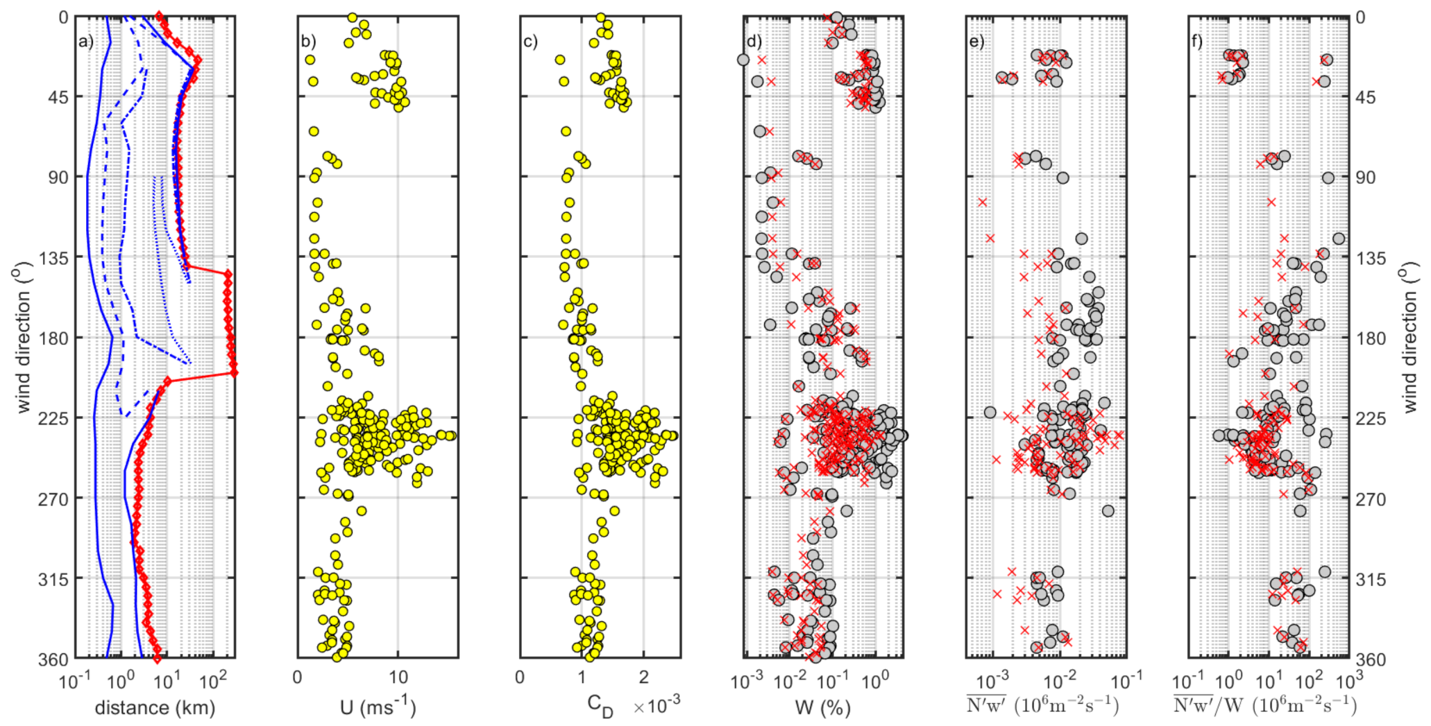
3.2. Aerosol Flux and White Cap Coverage by Wind Direction

Figure 3 shows a range of variables that define the measurement site (fetch, water depth, wind speed, drag coefficient, and white cap coverage) along with the measured particle flux as a function of the wind direction. This figure provides an overview of the whole dataset before a discussion of the individual wind sectors and particle size ranges in subsequent sections. Figure 3b,c shows that most of the high wind speed values and large drag coefficients were found in the southwestern near-coastal sector. In order to calculate the white cap coverage, we used the most common equation [7] for open sea white cap coverage:
W (%) = 3.84 × 10⁻⁴ × U3.41
where U (at 10 m) is the mean wind speed, and a white cap model that includes the effect of limited fetch Xf [52]:
W (%) = 0.06 × CD × U7/3 × Xf0.33
where the drag coefficient CD is
CD = k2 / (12.505 + 0.358 × ln(Xf) − 2.716 × ln(U))2
with k being the von Kármán constant (0.4). Obviously, W is influenced by Xf through both Equations (7) and (8), but in opposite ways. However, at small Xf, the dominating effect is to limit W to smaller values than predicted by Equation (6). The effect of this can be seen in Figure 3d, where W was calculated on the basis of measured U and Xf using both Equations (5) and (6). In the long fetch sector from 145° to 205°, both equations give almost identical results, while at short fetches, Equation (7) predicts roughly half the white cap coverage. This is in agreement with the physical reality where waters with limited fetch (such as lakes or sea water in offshore wind) require much larger wind speeds to produce the same amounts of white caps. Despite the effect of fetch, it can be seen in Figure 3d that the higher wind speed in the near coastal sector produced a higher white cap coverage at high wind speeds than did sectors with a limited fetch at low wind speed. Nonetheless, the use of Equation (7) reduced this difference. In Table 1, we can see that one effect of the fetch was to reverse the order between the coastal sector (0.23% white caps) and the Kalmar Strait sector (0.29% white caps), where otherwise the coastal sector with its higher wind speeds would have had the highest W. From here on, W shall exclusively be calculated using Equations (6) and (7), because it appears that the fetch considerably influenced our dataset, and that ignoring the influence of this on W would be unavoidable.
Figure 3e shows the upward aerosol flux. It can be seen that the largest fluxes (>104 m−2s−1) were found either at the high wind speeds in the near coastal sector or at the moderate wind speeds in the long fetch sector. It is interesting to note that while the long fetch sector and the Kalmar Strait sector both had larger average fluxes for the dry aerosol than for the non-volatile aerosol, especially the long fetch sector, in the coastal sector, there was no significant difference. This suggests that on average the entire sea spray flux for this sector was non-volatile. We can also see that the highest average aerosol number of emissions was found in the sector with the smallest average U and W, i.e., the long fetch sector.
In order to examine how these fluxes would compare if they were normalized to the white cap coverage, we calculated the upward flux per white cap area ( w N ¯ /W). It can be seen in Figure 3f and Table 1 how this increased the flux per surface area by a factor of 100–1000, since we moved to estimating the emissions per white cap surface and ignored the rest of the sea. The average non-volatile fraction was roughly half of the total number of emissions. This could be the result of internally mixed sea spray that shrink below the lower detection diameter of the OPC because semi-volatile organics are lost in the thermodenuder, or externally mixed sea spray where half the particle number is completely lost in the thermodenuder.

3.3. Aerosol Emissions by Size

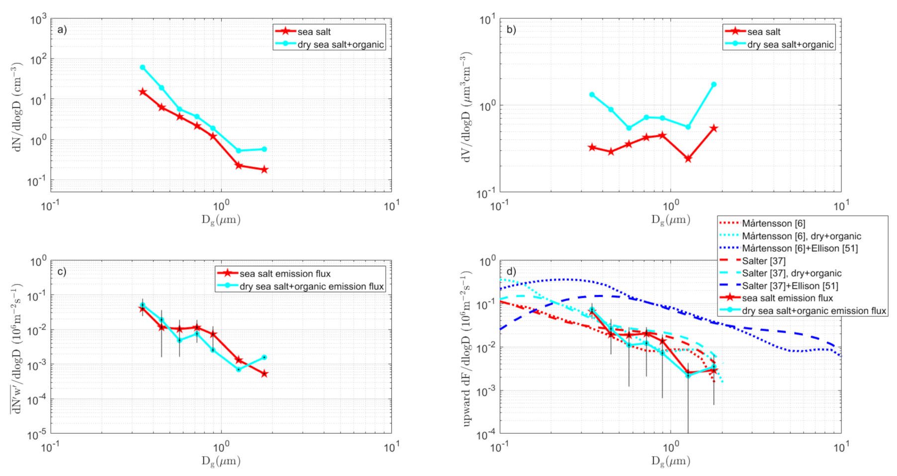
3.3.1. Coastal Sector

On average, the aerosol number size distribution in the coastal wind sector decreased in number concentration with increasing size by about two orders of magnitude from 0.3 to 2 µm diameter. The number concentration of the non-volatile fraction was about a factor 2–3 lower in concentration than that of the dry fraction, see Figure 6a. The nearly constant slopes as a function of the particle sizes were not broken until we reached super micrometer sizes. The volume concentration had a different behavior (see Figure 6b), where we probably saw the upper tail of the accumulation mode in the lower end and the beginning of a coarse mode in the upper end of the OPC range, while between them was a small mode centered at about 0.8 µm diameter.
The total average net aerosol number flux was dominated by the smallest OPC stage. The whole size range showed on average a positive (upward) flux, which indicated that sources were dominant over deposition. For the whole 0.3–2 µm diameter range, the dry and non-volatile aerosol fluxes were practically identical (see Figure 6c). The averages of only periods with net upward fluxes are shown in Figure 6d. On the log–log scale, these formed a continuous decline in the flux magnitude from 0.3 to just above 1 µm diameter, where the flux of the last size range increased in magnitude. Moreover, here, the dry and non-volatile fluxes were negligibly different when considering the average errors.
It may seem like a contradiction that the dry and non-volatile aerosol concentrations differed, while the corresponding fluxes did not. However, one must remember that the latter are turbulent fluxes, and only include those particles that have a correlation with the vertical wind because of a significant local source or sink within the flux footprint. Pre-existing aerosols with sources beyond the footprint such as ammonium (bu) sulfate and nitrates will at most contribute through deposition fluxes, which may cause a small underestimation of the emission fluxes that we corrected for when calculating the emission flux F from the EC aerosol fluxes w N ¯ . This is one reason that eddy covariance fluxes are such a powerful tool to study local primary aerosol sources such as sea spray.
What the small difference between the curves in Figure 6d suggests is that all of the sea spray aerosol in this sector were non-volatile, presumably sea salt. Alternatively, the proximity of the Swedish coast and numerous anthropogenic aerosol sources may have had the unfortunate effect that the dry aerosol flux suffered from a larger influence of dry deposition fluxes than the non-volatile aerosol flux, despite efforts to correct for this. This could have caused the difference between the fluxes to look smaller than it should have been, especially if there had only been local sea spray emission fluxes.
The sea salt aerosol size is proportional to the salinity in the water. In addition, we assumed that the original sea spray droplets at formation included so much water that their salinities were the same as in the local sea water (in other words, that sea salt was not enriched, a conservative assumption), which implies that at their creation they had diameters that were 5.2 times larger than those predicted by the Mårtensson and Salter parameterizations for the dry size at 7 ppt salinity following Equation (5) (dashed and dotted red curves in Figure 6d). Of course, these are likely to rapidly shrink in size and equilibrate with the surrounding relative humidity. The original size, however, is important if we are to estimate the potential organic surfactant fraction and accept the conclusion of Ellison [50] that surfactants carried by one droplet will be proportional to its original surface. We used the simple approach by Ellison [50] to estimate the contribution of a monolayer of organic surfactant molecules covering the sea spray, and then combined this with the Mårtensson and Salter models (see the dashed and dotted blue curves in Figure 6d). The monolayer of course also added to both the size and mass of the sea spray, insignificantly for larger particles, more so the smaller the particles were. When completely dry, the diameter of the remaining internally mixed sea salt/organic aerosol was represented by the dashed and dotted cyan curves in Figure 6d.
We can see that the measured unheated but dried aerosol concentration size distributions for both number and volume (Figure 6a,b, respectively) were larger than the heated non-volatile aerosol concentrations in the same figures. However, here, the difference between the curves for both unheated dry aerosols (cyan curve) and heated non-volatile aerosols (red curve) fell within the error bars. That is logical if the former would represent both sea salt and primary marine organics and the latter only sea salt, even though in reality these also include other aerosol sources. On the other hand, for the aerosol emission fluxes in Figure 6c, we know that the aerosol here originated only from the local footprint, and should therefore only be sea spray.
The reason for using three modifications onto source functions was to predict three situations. First, the pure sea spray flux with no organics was reduced to local Baltic salinity (red curves in Figure 6, Figure 7 and Figure 8). Second, the sea spray aerosol emission was enriched by organic matter and water just after ejection from the sea surface (blue curves on Figure 6, Figure 7 and Figure 8). Third, aerosol emission particles were enriched after evaporation by organic matter (cyan dotted/dashed curves).
For Figure 6d, we observed first of all that the two source parameterizations agreed with each other from about 0.5 µm to 2.5 µm diameter for the pristine droplets (blue curves). By “pristine” we mean that the droplets were at their initial creation size and had not yet adapted to the surrounding relative humidity. An organic monolayer might delay the evaporation of the pristine sea spray droplets somewhat. The important question is if it is long enough to preserve that water through the turbulent transport from the sea surface to the OPC in the EC flux system, and through the drying unit in front of one of the OPCs and the thermodenuder in front of the other OPC. Comparing the blue curves representing this pristine sea spray with the observed dry and heated aerosol flux distributions (full curves in Figure 6d), we found that this water was lost before entering the OPCs and that we were measuring the dried sea spray, sea salt, or sea salt + organics.
The 0.5 to 2.5 µm diameter range for the pristine droplets (blue curves) in Figure 6d corresponds to 0.2 to 0.5 µm dry diameter (cyan curves, sea salt, and organic surfactants).
Below this range, the Mårtensson model shows a higher emission, while above this range, the Salter model shows a larger emission of sea spray. This applies to the average wind speed and temperature for data in the coastal sector ( U ¯ = 7.6 m/s, mean water temperature = 13.5 °C). When comparing the observed heated flux (presumably sea salt only) with the Mårtensson and Salter sea salt parameterizations (red dotted and red dashed curves, respectively), we found that they fell within the error bars from about 0.4 to 1 µm dry diameter. If we similarly compared the parameterization curves for sea salt plus organic surfactants (cyan curves), we found that they fell within the range of the observed fluxes of unheated but dried (presumably salt plus organic surfactants) from about 0.3 to 1 µm dry diameter. However, most of the data points were just as close to the modelled sea salt emission curves as they were to the internally mixed sea salt organic emission curves in Figure 6d.
Generally speaking, for the coastal wind sector, all model estimates of the sea salt-only emission fluxes (heated non-volatile) and the model estimates of sea salt + organic surfactant sea spray emission fluxes (unheated but dried) that were corrected for salinity fall within the error bars of the measurements to which we compared them. Hence, we can say that the models agreed with the observations in the sub-micrometer size range, but we were unable to distinguish between the sea salt and organic content of the sea spray.

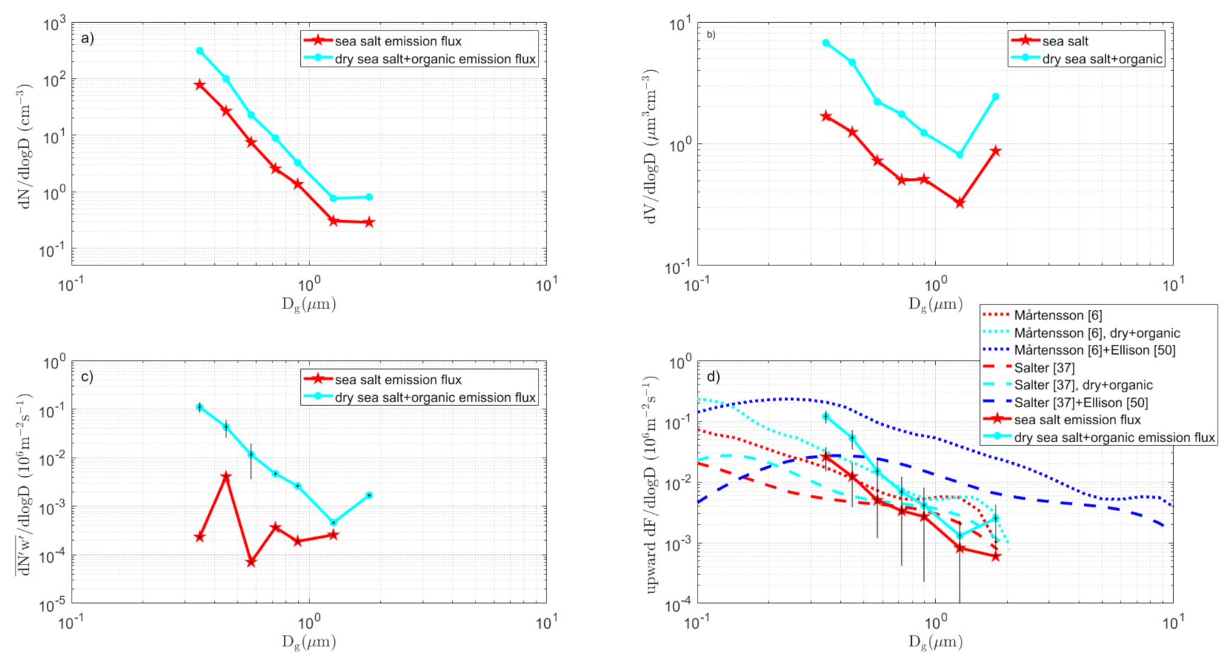
3.3.2. Long Fetch Sector

The southern long fetch sector is in many ways the most interesting, at least in terms of how sea spray emissions behave on conditions similar to the open sea. Compared to the coastal sector, we had similar aerosol number size distributions but with higher concentrations in the accumulation mode, while the volume size distribution lacked the irregular shape found in the coastal sector (see Figure 7c). The largest difference, however, was found in the net aerosol number flux size distributions (see Figure 7b). Here, the dry (unheated, cyan curve) aerosol flux was larger while the non-volatile (heated, red curve) aerosol flux was smaller than in the coastal sector. As a consequence, there were significantly larger dry aerosol fluxes than non-volatile aerosol fluxes. At least in the two smallest OPC channels, the dry and non-volatile aerosol fluxes differed significantly when considering the average errors. This implies that in the long-fetch sector, the sea spray emissions included substantial amounts of semi-volatile material, presumably organics, in addition to sea salt, especially in the low end of the size range.
When comparing these results to the Mårtensson [6] + Ellison [50] and Salter [37] + Ellison [50] models in Figure 7d, the picture is quite different than for the coastal sector (Figure 6d). For the heated non-volatile fluxes (presumably sea salt), the Mårtensson [6] curve (red dotted) was within the uncertainty of the observed values except for the size bin just above 1 µm dry diameter. The Salter [37] curve (cyan dashed) overpredicted the sea salt emissions below ≈0.4 µm dry diameter, but did well otherwise. The combined Mårtensson [6] and Ellison [50] parameterizations of the combined sea salt and organic surfactants (cyan dotted curve) were below the observed unheated dry fluxes (cyan solid curves) at about 0.5 µm dry diameter and again overestimated the fluxes just above the 1 µm dry diameter. The combined Salter [37] and Ellison [50] source parameterizations (dashed cyan curve) had the same problem, but underestimated the emissions even further in comparison with the observed fluxes (full cyan curve). The observed fluxes suggest that there was more material in the emitted aerosol particles than what could be explained by the sea salt and water-insoluble organics from the Ellison monolayer. These could be water-soluble organics, or surfactants, which formed micelles inside the droplets.

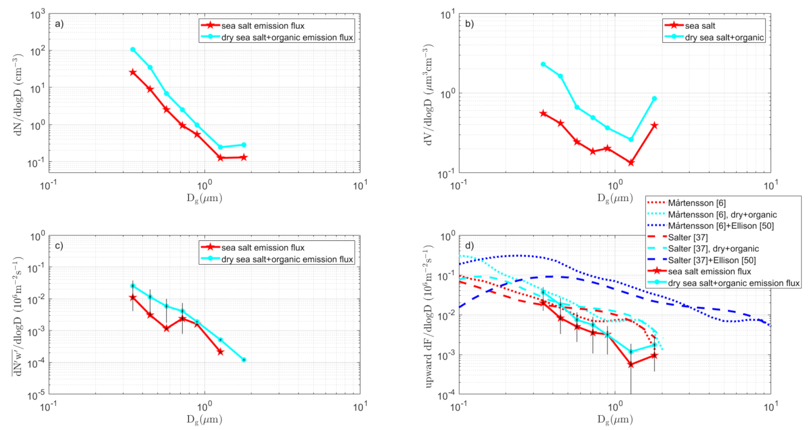
3.3.3. Kalmar Strait Sector

This sector shows that size distributions of concentrations and fluxes were somewhere between the characteristics of the other two sectors. The difference was between observed dry (unheated) and non-volatile (heated) aerosol EC fluxes w N ¯ , while emission fluxes (see Figure 8c,d, respectively) were even better separated from each other than for the long fetch sector. Just like the long fetch sector, the dry EC fluxes d w N ¯ / d D in Figure 7d increased exponentially with decreasing size, separating themselves from the heated number flux size distribution, and while they did so in the Kalmar Strait sector, it was much more pronounced. The resulting dF/dD were well separated from each other, and the errors did not overlap below ≈0.5 µm dry diameter. We shall further examine the chemical consequences for the sea spray source that resulted from this patter in the long fetch and Kalmar Strait sectors (see Section 3.7 and Section 3.8).
With regard to the sea spray parameterizations in Figure 8d, the aerosol flux size distributions of the Kalmar strait sector were partly reminiscent of the coastal sector (for the larger size bins) as well as the long fetch sector (the smaller size bins), but in general their results differed. The pure inorganic Mårtensson [6] parameterization (red dotted) fell within the uncertainty of the observed heated non-volatile fluxed (red solid curve) below ≈0.8 µm dry diameter, along with the Salter [37] parameterization (red dashed curve) below ≈0.5 µm dry diameter. For the combined sea salt parameterizations and Ellison parameterizations, both Salter [37] and Mårtensson [6] models agreed with the observed unheated fluxes of up to about 0.5 µm dry diameter.

3.4. Wind Driven Sea Spray Flux

Because the white cap coverage of the sea increases with wind speed [7], we did expect the sea spray emissions to do the same [24,25,26]. In Figure 9, we can see that this was indeed also the case for the sea spray aerosol fluxes in the coastal sector. For the other two sectors, we had too few data points and too narrow a wind range to find any clear trends in wind speed (see Table 1). Using a log linear fit between the mean wind speed and the aerosol number flux as in
w N ¯ = 10 k × U + m
the non-volatile fraction had both a better correlation with the wind speed (correlation coefficient r = 0.74 vs. r = 0.23), a stronger slope with wind speed than dry aerosol flux (k = 0.107 vs. 0.020), and a smaller zero bias (m = −2.81 vs. −2.06). In practice, the fit to the dry aerosol fluxes and the wind speed was not significant.
There are several possible explanations:
  • It may be that there is an organic semi-volatile fraction along with the sea salt that had a less pronounced wind dependency. The gradient flux measurements [53] suggests that the organic mass percentage of the sea spray would decrease with increasing wind speed (at the Irish west coast facing the North-Atlantic). It is however not straightforward to derive from that study how the number of emitted sea spray particles with organic in relate to the wind speed. Will the exponential increase in sea spray emission or the decreasing percentage of organic mass win, or lose, or result in a near steady state despite increasing wind velocity? The interpretation of Figure 9 in view of the results of [53] is further complicated because we do not know if the organic sea spray fraction and the sea salt sea spray fraction was entirely internally mixed. With at least a significant part of externally mixed organic sea spray, alternatively if bubbles scavenge relatively less organic surfactants at high wind speed we cannot exclude this possibility (see discussion further down in Section 3.8).
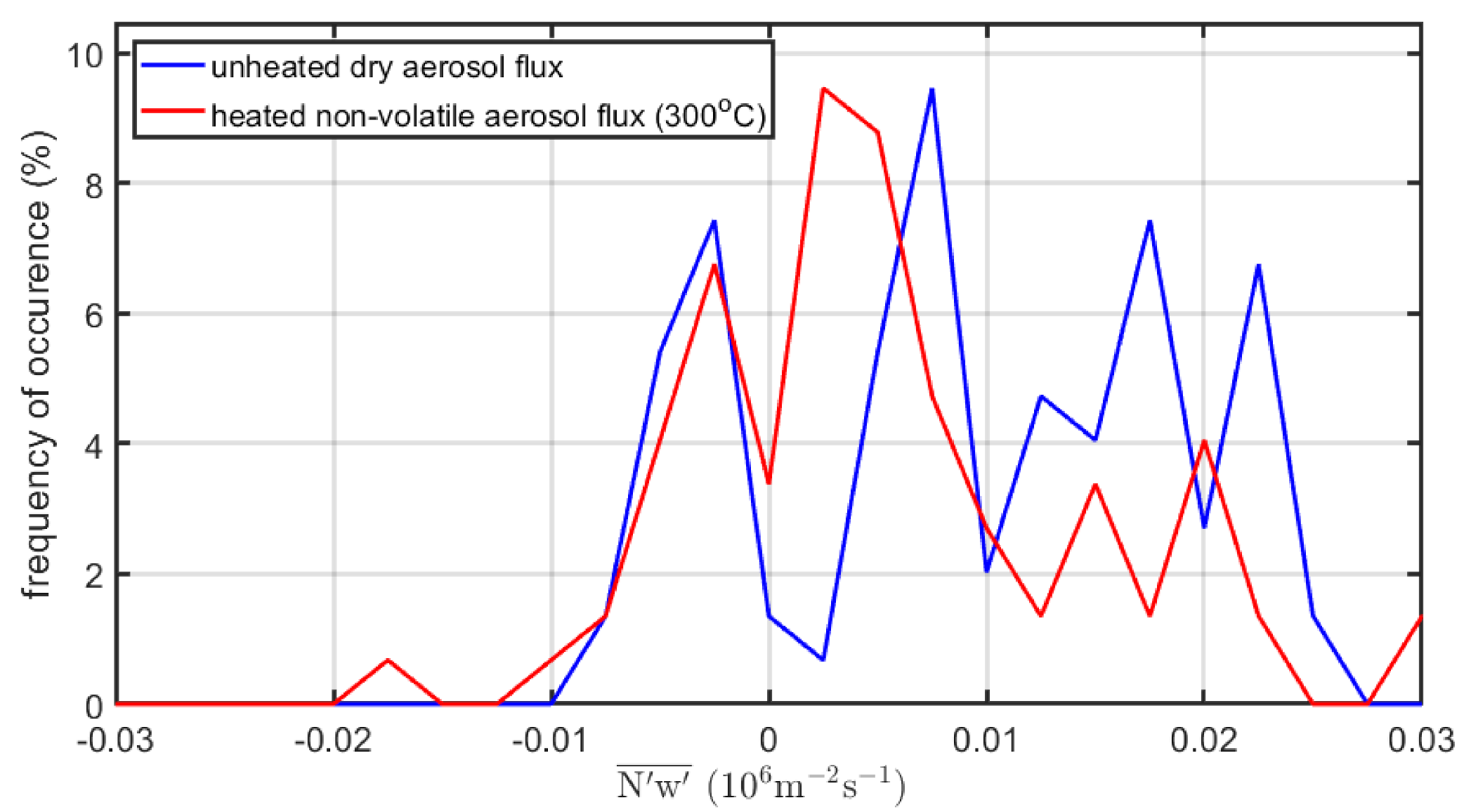
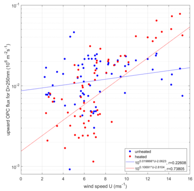
  • While previous studies (in the Arctic and Atlantic Oceans) have been in fairly remote marine regions, the data of the current study originated from a region with strong anthropogenic influence on the aerosol. We should expect that the dry aerosol concentration contained significant amounts of anthropogenic non-sea-spray aerosols. These would not covariate positively with the vertical wind since they do not have a source within the footprint. They may contribute to the flux with a smaller negative covariance due to deposition at the surface, but this is usually an order of magnitude smaller than the sea spray emissions. Dry deposition is usually considered to be wind-dependent as well, e.g., [8], which could obscure any wind dependency in the sea spray source flux. This should cause more scatter (and lower correlation coefficient), less pronounced slope to the horizontal wind, and a larger zero bias, as observed in Figure 9. The heated non-volatile aerosol would most likely suffer much less from anthropogenic influence, since at 300 °C the only remaining anthropogenic aerosol component would be soot (which is likely to primarily occur at smaller sizes considering their number).
The latter explanation is very likely to have played a role, and yet both effects could combine. It is not simple to distinguish between these two effects. As such, it is therefore not possible to conclude that the difference in wind dependency between the heated and unheated aerosol flux must have something to do with the difference in source mechanism in polluted areas such as the southern Baltic Sea. Unlike remote regions, the heating of the sampling line did not become a tool primarily to distinguish between the organic and sea salt sea spray components, but it was rather an essential tool to be able to separate the sea spray fluxes from other aerosol components.
If we compare the wind dependency of the sea spray flux from this study with previously published studies using Equation (9), it is clear that the heated (sea salt) aerosol flux in this study offered one of the best fits when taking into account both the correlation coefficient and number of data points. Its log-linear slope (k = 0.107) was very close to the slope calculated for the North Atlantic by [19] for unheated OPC concentrations >0.1µm diameter (k = 0.109). It also had the lowest zero bias value (m = −2.81) of all datasets thus far.

3.5. Ambient Diurnal Cycles

Figure 10 shows the average diurnal cycles in several key ambient in situ parameters for the coastal sector. We only used data when both fluxes and tank experiment data were available, since the intention was to later compare in situ sea spray emissions on the basis of EC fluxes and on the basis of the sea spray simulation tank data. The data were averaged in 3-h time periods. The other sectors did not contain enough data points to form an average diurnal cycle.
The average wind speed exhibited a maximum just after midday, and a nocturnal minimum (Figure 10a). This was pronounced in the white cap coverage due to its non-linear dependency on wind speed with daytime maxima just above 1% (Figure 10b). The aerosol number concentration, on the other hand, showed an afternoon minimum and a maximum before sunrise (Figure 10c). Both the dry and non-volatile aerosol number concentrations had similar cycles, but the former had a much larger amplitude. The smallest differences between dry and non-volatile aerosol number concentrations were found at the minima concentration close to noon. It is interesting to note that while aerosol concentration at sea often correlates with the wind speed, e.g., [24,54], it does not do so in this case. Instead, the diurnal cycle in terms of average aerosol concentration resembles those observed over continental forests due to daytime dilution in an increasingly deep boundary layer [23,46].
The aerosol number fluxes had completely different cycles. The dry aerosol had fairly constant number fluxes throughout the day with a weak maximum in the morning and a minimum in daytime varying between 1 and 2 × 10⁴ m−2s−1 (Figure 10d). The heated non-volatile aerosol number flux, on the other hand, had a strong diurnal cycle with a maximum average flux of about 5 × 10⁴ m−2s−1 near noon local time. Just before noon, there was a steep increase in the non-volatile flux, and thereafter the non-volatile flux remained larger than the dry aerosol flux, gradually declining until midnight. While the dry aerosol fluxes had no resemblance to the diurnal cycles of wind speed and white cap, it is obvious from Figure 10b,d that the non-volatile (sea salt) aerosol flux followed these parameters very closely in phase and amplitude, suggesting that we may see a local sea spray source.
It may appear counter-intuitive to observe larger fluxes for the heated aerosol than for the unheated one, as the process of heating the air is expected to remove aerosol particles. This was the case with the average aerosol number concentration in Figure 10c; however, fluxes behave in a different manner to concentrations. The magnitude of the fluxes is not primarily dependent on their concentration, but on how well such concentration correlates with the vertical wind speed. If we remove part(s) of the aerosol that have weak correlation with the vertical wind speed, or even opposite (negative) correlation, we may very well improve the correlation (and covariance, hence the flux).

3.6. Diurnal Cycles According to in situ Fluxes vs. Tank Sea Spray Production

In Figure 11, we compare the ambient in situ eddy covariance aerosol fluxes of Figure 10 with the artificial sea spray production tank experiments previously presented by [13,14]. However, we only include those tank data that coincided with flux data. As a result, our average diurnal cycles look slightly different than in [14], even though their main characteristics have not changed.
The water temperature followed a diurnal cycle with a minimum shortly after sunrise and a maximum in the afternoon (with an amplitude of about 1.5 °C), roughly in phase with the diurnal cycle in air temperature, indicating that temperature changes (Figure 11e) were driven by the radiation, heat budget balance, and solar radiation. Dissolved oxygen (DO) had a similar diurnal cycle, with a minimum before noon and a rapid increase to a maximum near saturation in the afternoon, followed by a gradual decline during the afternoon/evening/night (Figure 11a,b). The authors of [14] showed that the diurnal temperature cycle (which influences the saturation level, see Figure 11b) could not cause this DO variation, and instead it must to a large extent have been caused by biology—photosynthesis producing oxygen in the daytime causing near saturation (100% at about 7 mL L−1) in the afternoon before decline in photosynthesis allowed for respiration, ventilation, and chemical reactions to reduce the DO level towards night-time levels of 75–80% (at about 5.5 mL L−1). The average variations in salinity were small and did not show a clear diurnal cycle (Figure 11f). Together with the water temperature cycle, one can predict the surface tension σw of pure salt water [55] (see Figure 11g), which follows a weak diurnal cycle with a maximum between morning and noon and a minimum in the afternoon. It should be noted that this calculation neglects any effects of compounds other than water and sea salt, including organic surfactants. For example, unsaturated fatty acids such as palmitic and stearic acid are abundant in the ocean surface and enriched in marine aerosols [15,16,17,56,57], with surface tensions in the order of 3× 10⁻⁴ Nm−1 (http://ull.chemistry.uakron.edu/erd/, accessed on 17 February 2021), comprising less than half that of the “pure” sea salt sea water.
As described by [14], the average aerosol number concentrations in the tank experiments describe a clear diurnal cycle for both the CPC and OPC size ranges (see Figure 11c,d). High night and morning concentrations are followed by a rapid decline around noon and an afternoon minimum. Because the tank experiment excludes all sources other than sea spray, we can consider these number concentrations to be proportional to the sea spray production within the tank. In the OPC size range, the warmer temperature in the afternoon would cause less particle production and vice versa (for example, Mårtensson et al. [6] and Salter et al. [37]), but the magnitude of the temperature cycle is too small to explain the observed amplitude in aerosol production.
However, the question remains, how do these laboratory measurements compare with the EC fluxes? A direct comparison of Figure 11c,d with Figure 10d does not help. The average diurnal cycle in the in situ non-volatile aerosol number flux (which we may assume to be dominated by sea spray sea salt) with its strong noon maximum did not agree with the daytime minimum in the tank sea spray production. However, we concluded from Figure 10 that this maximum was caused by the wind speed, since the white cap fraction was used to derive the sea spray production in the tank. To be able to determine parameters of secondary importance, we tried to normalize the observed aerosol number emission fluxes with the white cap coverage, which has been the favored method in several past sea spray tank simulation studies to scale the tank data into in situ emission fluxes. The resulting diurnal cycle of w N ¯ /W in Figure 11h agreed even less with the diurnal cycles in aerosol concentration in the sea spray simulation tank (Figure 11d) than the in situ aerosol EC fluxes w N ¯ in Figure 10d.
The scaling to W cannot be considered successful. It demonstrates, however, that while the diurnal wind cycle creates one diurnal sea spray cycle with a daytime peak production, the actual production per white cap surface may have an opposite trend, caused by other factors than the wind speed. On the basis of the strong anti-correlation between the DO and temperature cycles, the authors of [14] proposed the hypothesis that the onset of photosynthesis, probably followed by increased respiration, may have resulted in the production or release of organic surfactants in the water. These may in turn have caused a decrease in particle production due to changes in the surface tension that follow from an increase in surfactant concentration. The comparison with in situ fluxes appears to offer partial support for this hypothesis. However, at this point we have no explanation for the difference in phase between the diurnal cycles of in situ and tank aerosol production.

3.7. The Complete Sea Spray Emission Size Spectra vs. Source Parameterizations

Sea spray emission fluxes have previously been measured in situ using direct flux measurements with the EC method and using a CPC or an OPC [18,19]. Due to the difficulties in measuring size-resolved number fluxes below the OPC range fast enough for EC (preferably 20 times per second but at least once per second), thus far, no one to our knowledge has been able to measure a complete sea spray emission size spectrum on the basis of in situ direct flux measurements. Differential or scanning mobility sizers (DMPS or SMPS) can reach as far down as a few nanometers in diameter, but require several minutes to scan all its size channels, rendering it inappropriate for the EC method. An alternative would be a DMPS run in a relaxed eddy accumulation (REA) system such as the one used over the boreal forest by [41], but that type of system is yet to be used for investigations other than deposition fluxes over the boreal forest. There are alternative methods for detecting and sizing the aerosol in this size range at a speed of several hertz, e.g., [58]. Unfortunately, instruments such as electrical low-pressure impactors (ELPI) are expensive and/or require high aerosol concentrations, which might be why they have not been applied to the sea spray problem. The authors of [59,60,61,62] tried to cover the whole sub micrometer spectra using an indirect method, deriving the fluxes from gradient measurements and letting the surf zone represent breaking waves. The most important uncertainty with the study by [59] is probably the question of whether or not the surf zone sea spray production is really representative of the open sea’s breaking wave sea spray. One can also consider laboratory experiments, such as the classic experiment by [7], although this one only covered particles corresponding to >1.1 µm dry diameter. The more modern study by [6] covered all of the sub-micrometer size range, even though indirect methods and Equation (6) were used to derive the oceanic sea spray emission flux. While these methods are sometimes the only technically available means of obtaining certain required information, they are also associated with certain uncertainties related to the limitations of the methods. For example, are the bubble spectra in the tank representative of the open sea? Are the dimensions of the tank sufficient to avoid wall effects? How do we scale to the in situ ocean?
Therefore, a different approach was planned for this experiment that combined both a direct and an indirect method. We allowed the experiments producing artificial sea spray in local sea water that have already been published by [13] to provide us with information on the sea spray size spectra produced below the OPC size range ([13] used a DMPS system), and we used the direct EC flux measurements presented in the current study to determine the magnitude of the sea spray production. The two datasets can be combined because they overlap in the size range 0.3–2 µm dry diameter, where both systems included an OPC from the same manufacturer (Grimm) with the same properties (see Figure 12). As with comparing the diurnal cycles in Figure 10 and Figure 11, we only used periods for which both tank and EC data were available, and we excluded periods with <4 ms−1 to forestall influence from waves breaking against the coast.
First, we took the full DMPS and OPC number size spectra from the sea spray production in the tank and scaled them into the same units as the EC fluxes (106 particles m−2s−1) by multiplying the particle concentration in each bin with the sample air flow from the tank to the aerosol instruments (q = 6.3 lmin−1) and then dividing by the tank water cross section surface (A = 6.16 × 10⁻² m2). In principle, in this we assumed that the particle production by bubble bursting would result from the entire water surface in the tank. We had no continuous photographic log of the surface, and that was an improvement that we did not add until we used the more advanced system used and described in [37]. However, from ocular observations during the experiment, we know that this surface was completely covered by bubbles at least some of the time.
It is at the next step that many similar bubble–sea-spray simulation tank studies such as [6] have scaled the particle production per surface and second to in situ fluxes using one of the parameterizations for the ocean white cap coverage, such as Equation (6), for scaling of the tank water surface covered by bubbles to the white cap coverage of the real ocean. That would result in an emission flux, not per white cap area, but from the entire ocean surface, just like an EC flux system detecting particle fluxes from its entire flux footprint area. Unfortunately, there are large uncertainties associated with determining both the tank’s proportion of water covered by bubbles, as well as with the photographic method used to derive in situ W. This is not only associated mostly with the large area error when using a camera slightly elevated above the ocean to photograph the ocean surface at small angles, but also due to the method’s sensitivity to what brightness value is used to separate white cap surface from the ocean surface. There is also a principal problem if at all the surface of bubbles on the tank water surface corresponds to the white cap coverage.
Comparing with the values calculated for W in Figure 3 and Table 1, we found it obvious that scaling with W could not solve our problem. Using W would not match the magnitude of the in situ aerosol emission fluxes to the tank sea spray production (if we also assume a tank water surface completely covered by bubbles and corresponding to 100% W). However, we were not entirely surprised by this, and as the goal was to tune the tank data to simultaneously measured in situ aerosol EC fluxes, we needed to search for another solution.
A few recent studies have used air entrainment or energy entrainment to scale the tank experiment’s particle production to in situ emission fluxes. Entrainment in the tank can be measured, and is better defined than as “white caps” in a tank. Entrainment over the ocean has also been quantified as a function of wind speed or friction velocity (u*) [63]. Following [37], this can be used to scale the production in a sea spray tank experiment into in situ sea spray emission fluxes. Unfortunately, entrainment was not measured during the Garpen experiments.
We therefore tried a new approach. Considering the EC aerosol fluxes to be the most accurate quantification of the in situ sea spray emission fluxes available to us, we tried to directly scale the sea spray tank simulations to the former. First, we recalculated the magnitude of the tank particle production per tank surface and time into particle production per ocean surface and time. We did this simply by scaling the sea spray production counted by the OPCs in the sea spray tank to that of the EC system at the smallest OPC size bin (which had the highest count and smallest errors) using the EC system OPC as the reference so that they matched each other. The scaling factor we derived in this way was 0.0931. It was smaller than 1 because the tank particle production per surface and time was larger than the actual in situ emission flux that we observed. If we tried to scale to one of the larger size bins of the OPC’s, the entire range of possible scaling factors would be from 0.0078 to 0.0931, depending on which size bin we used for the tuning, which would decrease with larger particle sizes. This additional range of uncertainty stems from our inability to match more than 1–2 size bins at the time between the tank sea spray simulation and the in situ sea spray eddy covariance fluxes. This in turn issues from one of the most obvious results in Figure 12—these two methods give rise to different slopes of the sea spay size distribution at dry diameters larger than ≈0.5 µm.
Compared to values calculated for W in Figure 3 and Table 1, it is obvious that scaling with W could not match the magnitude of the in situ aerosol emission fluxes to the tank sea spray production (if we also assume a tank water surface completely covered by bubbles and corresponding to 100% W). However, we were not entirely surprised by it, and as the goal was to tune the tank data to simultaneously measured in situ aerosol EC fluxes, we proceeded along that path.
We added the observed EC aerosol emission fluxes as cyan-filled green circles with vertical bars representing the 10% to 90% percentiles. Finally, we could use Figure 12 to compare the degree to which the indirect emission estimate based on the bubble tank data agreed with the in situ aerosol EC flux measurements. The sea spray emissions had broad peaks centered at 0.09 and 0.3 µm diameter. The method we chose in order to scale the tank data to the in situ fluxes only managed to exactly match the magnitude of the EC aerosol flux data at between 0.3 and 0.4 µm dry diameter because we used that size bin for the tuning. From there and upward in size, the measured/estimated aerosol sea spray production by the two methods deviated significantly. It became obvious that the slopes, as a function of increasing particle size diameter, differed for the two methods. The tank experiment produced a curve with a less downward slope but with increasing particle size than the real in situ fluxes observed with the EC method. As a result, the sea spray production in the tank could have been larger than the aerosol EC emission fluxes in this range, with the scaling factor represented by the green-blue diamonds in Figure 12 (in the 0.6–1 µm dry diameter, 90% of the fluxes derived from the tank measurements were larger than 90% of the EC). However, if we consider how uncertain we were about that scaling factor, the entire aerosol EC flux curve fell within that uncertainty (the bright green shaded area).
Figure 12 also includes to the source parameterizations of sea salt sea spray emission fluxes from Mårtensson [6] and Salter [37], adapted for the lower salinity (in our case, 6.8 ppt on average) as in Figure 6, Figure 7 and Figure 8, and adding the volume of an organic surfactant layer according to Ellison [50], in order to make them represent the total sea spray emission fluxes, as intended in Figure 6, Figure 7 and Figure 8.
Comparing the parameterized total sea salt + organic curves with the observed emissions (both those directly measured with the EC method and indirectly estimated from the tank experiments), we can see that both of the parameterized sea salt + organic dry aerosol captured the magnitude of the largest sea spray production, and although Mårtensson + Ellison [6,50] captured the ≈0.1 µm peak very well, it missed the 0.3 µm peak, while Salter + Ellison [37,50] had its peak in between at about 0.2 µm dry diameter. Mårtensson + Ellison [6,50] overestimated the magnitude of the peak sea spray production somewhat, especially at the smallest sizes to the left of the peak production, whereas the Salter + Ellison [37,50] parameterization underestimated the peak production level, more so at the smallest sizes. Salter + Ellison [37,50] then declined over increasing diameter with a lower slope, such that it captured the overall slope of the observed sea spray emissions, but somewhat below them at up to 0.25–0.3 µm dry diameter. While the Mårtensson + Ellison [6,50] method showed a steeper slope with increasing diameter, which better matched the observed slope of the EC aerosol fluxes, from about 0.3 to 0.9 µm and at 2 µm dry diameter, it also landed very close to the actual magnitudes of the EC fluxes.
In summary, on the basis of Figure 6, Figure 7 and Figure 8 and Figure 12, we found that above ≈0.8 µm dry diameter, there was no significant difference between the sea spray emission fluxes derived from the EC method in the current manuscript when taking errors into account as well as the two sea salt source parameterizations. Below ≈0.8 µm dry diameter, differences between the two sea salt source parameterizations were most likely due to difference in bubble production, which resulted in a much less realistic bubble spectra in Mårtensson [6], and the much smaller bubble tank in Mårtensson [6], which could lead to considerable wall effects and a distorted bubble spectrum on account of the enhanced coalescence along the walls and increased bubble bursting on the water surface. Below 0.8 µm dry diameter, the most pronounced differences between the experiments in this study and the sea salt source parameterizations were likely to have something to do with the fact that [6] and [37] were made with artificial sea water without any organic content, while this study with in situ-sampled water added the entire chemical complexity of real sea water. It is true that we tried to add the organic mass fraction to the sea salt using the Ellison [50] model on top of the sea salt parameterizations. However, that does not consider the possibility that organic surfactants on the water or bubble surfaces influence the actual sea spray formation process and redistribute both sea salt and organic mass over the sea spray size distribution. This sort of effect is most likely to be found where there is the biggest discrepancy between the source parameterizations and the observed sea spray production: <0.15 µm dry diameter for Mårtensson [6] and <0.1 µm dry diameter for Salter [37]. At this stage, it would be pure speculation on our part to guess exactly how this would work. We know, however, that the surface tension of the water changes much more from a small amount of organic surfactants than from either water temperature or salinity, and surface tension is deeply involved in how and when bubbles burst.
If we would choose to scale the sea spray tank data to the EC aerosol fluxes at a different OPC size bin, the comparison of emission magnitudes obviously changes, but with two observations unaffected by the scaling:
(i)
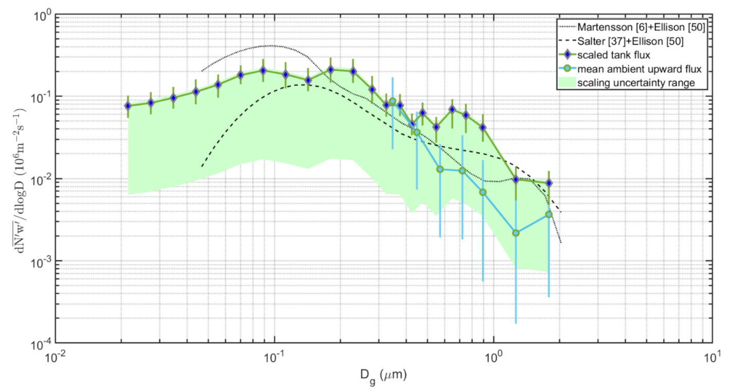
The difference in slope over aerosol size between the tank sea spray simulation and the direct in situ EC fluxes remains.
(ii)
The conclusion that sea spray is produced in a wide sub micrometer range, centered and peaking at about 0.09–0.3 µm dry diameter is not affected by the scaling.
This first attempt to extend the observations of sea spray production by bringing laboratory sea spray tank simulations out into the field and feeding them with local in situ water may at first seem like a failure or disappointment. However, given the uncertainty caused by the scaling that we do, and within the errors and variability of the dataset, we nonetheless found a fair agreement between two experimental methods and two source parameterizations within a range of about 0.1–2 µm dry diameter. For further use of this strategy, it would be important to strive towards reducing the uncertainty in how we scale the tank experiments to the in situ direct flux measurements.

3.8. Chemical Interpretation of The Semi-Volatile/Non-Volatile EC Flux Fractions

We estimated the percentage of organic sea spray fraction to the total sea spray emissions, on the basis of our EC aerosol flux measurements. These build on assumptions that the fresh sea spray is either externally or internally mixed (see Figure 13). Since we measured both the heated non-volatile aerosol EC fluxes (presumably sea salt) and dry unheated aerosol EC fluxes (presumably containing all components except water), we thus were able to, as in Figure 6, Figure 7, Figure 8, estimate the organic fraction. If we assumed an external mixture, it was simply the difference between dry unheated and heated (non-volatile) aerosol fluxes, divided by the dry unheated aerosol EC fluxes for each size bin. To estimate the organic fraction for an internally mixed sea spray, we must shift the aerosol number flux size distribution bin by bin from the dry unheated aerosol size distribution to the heated non-volatile distribution. This is presumably a shift from the total (organic + sea salt) size distribution to a pure sea salt distribution, and then use the required size shift as an estimate of the semi-volatile, and presumably, organic fraction. The operation includes interpolation of the shifted size spectra in order to be able to compare values at the same diameters. Figure 13 includes the percentage organic fraction derived from our EC aerosol flux data while assuming an internally and an externally mixed aerosol. Included in Figure 13 are also the ambient aerosol impactor data from the Irish west coast observed by Cavalli [64], one of several publications based on data from the Mace Head station, where the water-insoluble organic mass fraction was divided by the sum of the water-insoluble organic mass and the sea salt mass. There were also data from a field tank experiment using local water in the Bermuda Sea, wherein a mass spectrometer is used to decide the organic fraction of the sea spray by size [65]. Facchini [31] took an important step by repeating similar measurements at Mace Head as Cavalli [64] (blue dashed curves), but simultaneously sampling and analyzing the sea spray aerosol produced in our sea spray tank using local water on board the research vessel (RV) Celtic Explorer on the North Eastern Atlantic Ocean, upwind from the Mace Head station (blue dotted curves). It established that the size distribution of organic vs. sea salt sea spray found in ambient air was identical to the one found in sea spray tank experiments, where sea spray is known to be the only source, which supports the conclusion that these size distributions are a signature of sea spray. All these experimental measures of the sea spray chemical composition by size suggest that there is a shift in the composition from predominantly sea salt in the super-micrometer to predominantly organic compounds at around 0.1 µm diameter with a transition region in between. The ambient as well as tank sea spray aerosol size distributions by [31,64,65] agree fairly well with each other, as well as with the conceptual “mono-layer” model suggested by Ellison [50]. Keene [65] had a size shift slightly to the left of the other data and of the Ellison [50] curve, but qualitatively showed a similar size shift.
With this study, we have shown that EC aerosol fluxes combined with a thermodenuder can derive similar information about the organic vs. sea salt distribution in sea spray as traditional chemical methods. The use of EC fluxes places our method closer to the sampling and analysis of the sea spray from sea spray tanks by [31,65] than the ambient impactor samples and chemical analysis by [31,64]. This is because when using the EC method, we know that the detected aerosol flux originates from the upwind turbulent flux footprint, which is typically a few hundred meters, and at most a kilometer. Hence, we know that we are studying a freshly born sea spray aerosol. In this way, we have with these new data added further support to the conclusion made in [31], that this shift between dominantly sea salt and dominantly organic mass between 0.1 and 1 µm diameter is a signature of the sea spray aerosol. While it is very useful to see that an aerosol EC flux system with a built-in thermodenuder is able to separate the organic sea spray from the salt sea spray, unfortunately our data are roughly and equally consistent with an externally as with an internally mixed sea spray aerosol. However, an internal distribution would be consistent with the Ellison [50] model. Perhaps if we add more similar data, we may be able to draw final conclusions about the state of mixture of the sea spray.
The laboratory experiments by [6] suggested that lower salinity simply means that the aerosol size spectra shifted to smaller sizes proportional to the cubic root of the salinity. On this basis, we suspected that artificial sea spray experiments on Baltic waters would result in a size spectra centered at smaller sizes than in ≈35 ppt water. Instead, we saw size spectra centered at the same sizes as the saline oceans or the tank experiments with ≈35 ppt pure salt water (see Figure 12). The model approach in Figure 12 gives one possible explanation. If the organic fraction, or at least an important part of it, is determined by the surface area of the original droplets, as suggested by Ellison [50], and these droplets have the same salinity as the sea water, less salinity does not imply less organics. Less salinity means more water but may still imply roughly the same droplet surface at formation, which maintains a large fraction of organics in the mono layer, meaning that the final dry size does not decrease. In addition, if there are more organics than a mono layer with organic surfactants can explain, it would also contribute to the sea spray size. This, however, remains speculation until we have both detailed laboratory studies of the effect of salinity on sea spray formation, and more data in general on the organic sea spray fraction.

4. Summary and Conclusions

The main results and conclusions drawn from this study are as follows:
  • We have presented the first ever sea spray aerosol EC fluxes at near-coastal conditions and with limited fetch, and the first over a water surface with low salinity. Under these conditions, increased wind speed produces more sea spray than usual, and the emissions approximately follow the wind power law, that is, these exhibit a strong non-linear response to increase in wind speed. This compares reasonably well with previous studies from remote open oceans with normal salinity.
  • It is, however, only the heated non-volatile (sea salt) aerosol fluxes that show a highly significant increase in wind speed, similar to what we have come to expect from sea spray EC fluxes. Considering that this is a much more polluted region compared to the remote oceans where previous studies had taken place, the dry unheated aerosol fluxes probably include too much semi-volatile anthropogenic aerosols (which contribute negative deposition fluxes that may mask the emission fluxes, not to mention increasing the random errors). This emphasizes the importance of including a volatility system, a thermodenuder, in EC aerosol flux systems when studying sea spray emissions in polluted regions.
  • It was not trivial to combine tank and EC flux data into a continuous sea spray emission size spectrum from 0.01 µm to 2 µm diameter. We are unable to be conclusive regarding the scaling factor between the fluxes derived from the tank measurements and EC fluxes. The primary reason is that it appears both tank-derived fluxes and EC fluxes have different slopes over the aerosol size. Future work is needed to study if this is a feature related to the different methods used, and if it can be overcome.
  • Differences between various sectors (Table 1) in the particle production per white cap area were relatively small (2.2 – 2.7 × 10⁷ m−2s−1), which suggests that the approach by [6] and many others (to parameterize the sea spray emissions per white cap surface separately from the white cap cover wind-function) is a reasonable simplification. This was contradicted by the scaling of our tank-derived fluxes to our EC fluxes (Figure 12), which resulted in a range of scaling factors that cannot be explained by the white cap fraction vs. tank bubble surface. There were most likely other complications that may add to the uncertainty in the scaling between tank experiments and in situ fluxes. We had hoped that this problem would have been circumnavigated if one scales the tank sea spray simulations to actual in situ EC fluxes, as we have done in this study. However, as noted above, because the two methods resulted in sea spray emission fluxes with different slopes over aerosol size, we still had problems to resolve.
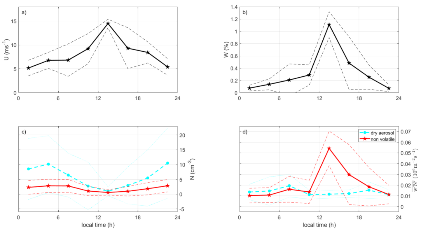
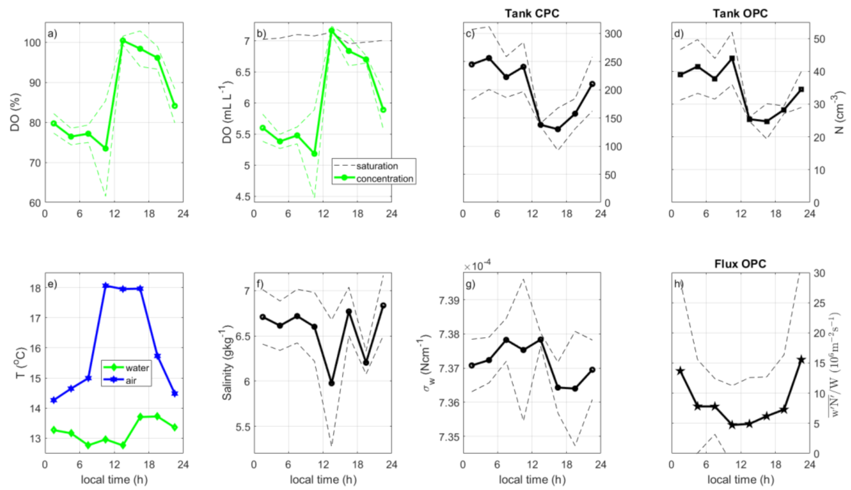
  • Diurnal cycles for in situ particle production were closely related to wind speed and white cap coverage, with maxima at around noon. Tank sea spray production had an afternoon minimum in their diurnal cycle. In situ sea spray production changed from a peak at noon to a minimum at noon when normalized to the production per white cap area. Although with somewhat different timing, the diurnal cycles supported the existence of a biologically driven diurnal cycle in the sea spray production as suggested by [13], where the dissolved oxygen indicated a connection to photosynthesis or respiration.
  • Surprisingly, there appeared to be less organic sea spray production from the shallow waters in the coastal zone and Kalmar Strait zone than in the long fetch zone. It may well be that this is an artefact due to negative deposition fluxes of anthropogenic particles embedded in the upward net fluxes.
  • In the long fetch zone, we were able to distinguish between observed aerosol emission fluxes of dry aerosol (unheated, both sea spray and organics) and non-volatile aerosols (heated, sea salt only) in the smallest size bins of the OPC. This did not apply to the fluxes from shallow and coastal waters. The long fetch zone aerosol flux size distributions and organic fraction were in agreement with previous studies, but we were unable to conclude if the organic and sea salt sea spray in the OPC range occurred as internal or external mixtures. Both are equally plausible.
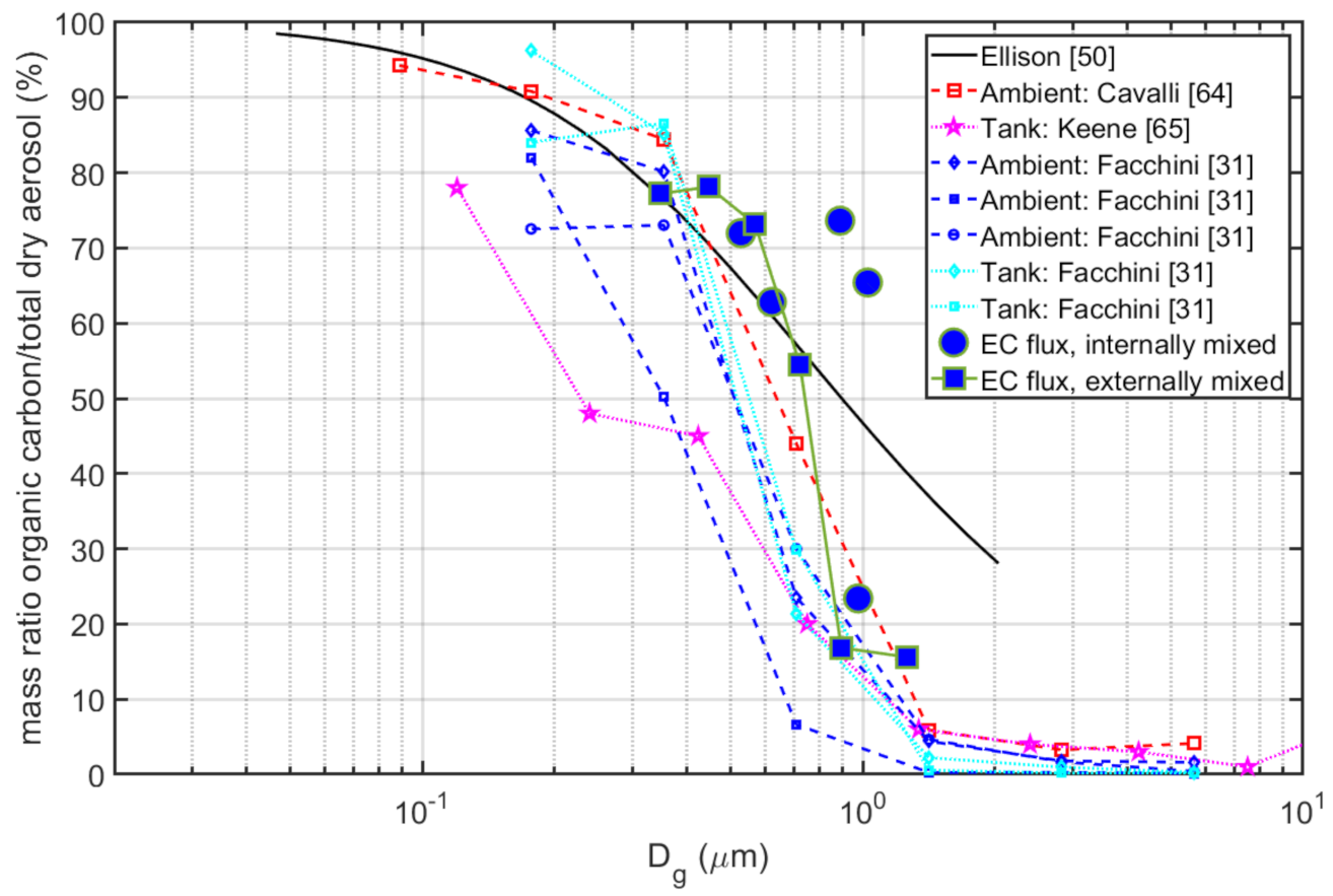
  • In our study, our estimates of the relative organic sea spray distribution over size using the EC method in combination with a thermodenuder demonstrated that this combination of methods was able to distinguish between organic and sea salt sea spray. It also confirms the conclusion by [31] that the shift from a predominantly sea salt mass in the super micrometer to a predominantly organic mass at ≈0.1 µm diameter is a signature of the sea spray aerosol.
  • As a first guess, over sea spray emissions from a brackish water such as the Baltic Sea, in both [6] and [37], sea salt source parameterization appeared to work, as long as the fluxes were modified for the actual salinity by shifting the particle diameters proportionally to the cubic root of the salinity, as suggested by [6].
  • The Ellison [50] organic mono-layer model appears to be able to explain most of the differences we observed between the dry aerosol and heated non-volatile aerosol. However, the rate of change in organic fraction over aerosol size, as suggested by [50], appeared somewhat smaller than most observations, including this study (see Figure 13).
  • The observed particle production by size was somewhere in the vicinity of both pure sea salt models [6,37], when these were modified for the salinity and simple surfactant monolayer model, as in [50]. In some sectors and size intervals, the emissions were even larger, and water soluble organics or liquid colloidal micelles within the droplets/particles could have contributed to the organic fraction. In most cases, we were not able to be conclusive due to uncertainty in the flux measurements.
Several contradictions and problems remain, which will require further studies to solve. Can we account better for the influence of deposition fluxes on the dry aerosol? Is the tank design or size responsible for the difficulties of matching in situ EC fluxes and tank sea spray production into one combined picture? We can note that the sea spray simulation tank used in this study was considerably larger than that used by Mårtensson [6], but much smaller than the more advanced sea spray simulation tank used by Salter [37]. Yet, it is the oldest of these studies (Mårtensson [6]) that best matched the magnitude and slope of the EC sea spray aerosol number flux emissions from about 0.3–1 µm dry diameter, while overestimating the flux < 0.15 µm dry diameter (see Figure 12). We have good reasons to believe that our experimental development from 2003 (Mårtensson [6]), over 2005 (this study), over several other publications, to 2014 (Salter [37]) has shown a consistent improvement in how realistically we can simulate sea spray formation in laboratory tanks. However, from the comparisons made in this study (mostly Figure 6, Figure 7 and Figure 8 and Figure 12), that does not appear to be the key to how well the laboratory sea spray tank simulations agree with the EC sea spray aerosol emission fluxes.
What are the biological and chemical processes behind the diurnal cycle in the sea spray production? How do these influence the sea spray composition and sea spray emission? To answer these questions, we probably need more advanced biochemical/organic microbiological analytical methods, such as those applied in [15,16,17]. It would be very interesting to see methods that allow such detailed chemical (organic) and microbiological characterization to be applied in a sea spray simulation tank that is tied to simultaneous in situ EC aerosol flux measurements.
Indeed, the basic approach of this study is to combine aerosol EC fluxes, which determine the magnitude of the in situ emissions, with more detailed measurements of the artificial sea spray formed in a laboratory tank using local sea water, in order to characterize properties that cannot be measured directly as EC fluxes. Can this approach be improved or replaced by another or a modified method so that we can reduce uncertainty and be more conclusive regarding the organic fraction and its state of mixing with the sea salt, thereby achieving a complete aerosol sea spray flux size distribution? Perhaps the answer will in the end be to apply faster instruments than typical DMPS or SMPS systems to size the aerosol below the OPC size range, instruments that both cover the entire size range and are fast enough to apply the EC flux method. That would solve the problem of observing the complete sea spray aerosol emission size spectra. Even if that can be done, there remains the need to characterize the chemical composition of the sea spray in more detail than what the EC method with a thermodenuder can do, offline chemical analysis of specific organic compounds for example, as well as the biological fraction of the sea spray. If we are to base future emission parameterizations of the organic sea spray and of biological sea spray particles on direct flux measurements, the available analytical options (such as those in [15,16,17]) are not fast enough for the EC method, perhaps with the exception of the use of aerosol mass spectrometry in EC flux systems, which is still in its infancy. Eventually, it may well be that the so-called relaxed eddy accumulation (REA) method is an option that allows for in situ flux measurements of specific organic compounds and biological particles. The REA method is a micrometeorological method that allows for the use of slow instruments/sampling systems, and still produces a flux with the help of fast measurements of the vertical wind and some empirical tricks. It is frequently used for gas fluxes, but to our knowledge, there has only been one REA system for aerosol particles [41], for which the reason is probably the complications that follow from our need to use obviously inflexible tanks in stainless-steel for the accumulation of sampled air instead of flexible Teflon bags for gas flux applications, since aerosols are rapidly lost to Teflon surfaces. However, while waiting for technical and methodological progress regarding aerosol instruments and aerosol REA applications, we believe that a combination of EC fluxes and sea spray tank simulations is still worthy of application and elaboration for parts of the sea spray properties that cannot (yet) be studied directly as fluxes using the EC method alone. If the current COVID-19 pandemic does not prevent us, we have two cruises scheduled for 2021 where this approach will be revisited, but with more detailed and complex instrumentation than in this study. We hope the results of that field work will answer some of the questions left unanswered in this study.
Our main objective is to improve the available sea spray source parameterizations used in large scale models, including global climate models. The most urgent needs for improvements concern the organic and biological fractions of the sea spray emissions. To achieve that goal, we have to empirically determine the sea spray emissions as a function of a few fundamental parameters, simple enough for the code to be used in a gridded global model running up to 100 simulation years or more, but yet accurate enough to describe how sea spray emissions respond to changes in parameters that likely will change in a changing climate, such as wind speed, sea ice, water temperature, chemical composition of the water, and microbiology. With that goal in mind, the experimental approach used in this study is worth repeating at different locations and with improved experimental design and analytical methods. If the goal is to study the detailed processes, in situ data such as those in the current study may be too complex, such that one should attempt more controlled laboratory experiments with artificial sea water spiked with organic surfactants or controlled bacteria cultures. Further progress in this area is probably dependent on a combination of well-planned laboratory experiments and in situ experiments. For the in situ experiments, we would encourage other research groups to combine in situ tank experiments with EC aerosol fluxes. The latter is the only measurement actually able to constrain the magnitude of sea spray emissions, a feat not possible in sea spray tank simulations, neither in the laboratory nor in the field.

Author Contributions

Conceptualization, E.D.N.; methodology, E.D.N and E.M.M.; software, K.R. and E.D.N.; validation, K.A.H.H. and E.D.N.; formal analysis, R.K. and E.M.M.; investigation, E.D.N., E.M.M., and K.A.H.H.; resources, E.D.N. and R.K.; data curation, K.A.H.H; writing—original draft preparation, K.A.H.H. and E.D.N.; writing—review and editing, E.D.N. and P.M.; visualization, E.D.N. and P.M.; supervision, E.D.N. and R.K. All authors have read and agreed to the published version of the manuscript.

Funding

This research was financed by the European Commission, grant ID 18332, Swedish Research Council (VR), project numbers 622-2003-1120 (VR researcher position), 621-2003-3461 (equipment), 621-2003-3456, 2006-5050, and 2018-04255, and the Swedish Research Council for Environment, Agricultural Science and Spatial Planning (FORMAS), project number 2005-1540. Furthermore, this research was supported by the Polish National Agency for Academic Exchange under the Bekker Program (decision PPN/BEK/2019/1/00043/DEC/1).

Institutional Review Board Statement

Not applicable.

Informed Consent Statement

Not applicable.

Data Availability Statement

The data presented in this study are available on request from the corresponding author.

Acknowledgments

The authors gratefully acknowledge the NOAA (National Oceanic and Atmospheric Administration) Air Resources Laboratory (ARL) for the provision of the HYSPLIT transport and dispersion model from the READY website (https://www.ready.noaa.gov), and the Kljun flux footprint model (http://footprint.kljun.net/) that were both used in this publication. We would like to thank the foundation “Garpens Vänner”, which maintains the lighthouse on Garpen, for kindly letting us use the island and the lighthouse during the period of investigation and for help with logistical solutions. Valuable help was also provided by Hamish Struthers and Juri Wahler. We thank three anonymous reviewers for helpful comments and suggestions.

Conflicts of Interest

The authors declare no conflict of interest.

Notations

Naerosol number concentration, cm−3
N ¯ half hourly average aerosol number concentration, cm−3
N’turbulent fluctuation in aerosol number concentration, cm−3
wvertical wind speed, ms−1
w ¯ half hourly average vertical wind speed, ms−1
w’turbulent fluctuation in vertical wind speed, ms−1
w N ¯ turbulent aerosol number flux, eddy covariance flux, m−2s−1
Faerosol emission flux, m−2s−1
Fmmeasured turbulent aerosol flux limited by the sensor response time, m−2s−1
Fcaerosol flux corrected for limited sensor response, or aerosol emission flux, m−2s−1
τcfrequency first order response time constant, s
nmnormalized frequency
zmeasurement height, m
LMonin–Obukov length, m
U ¯ mean horizontal wind speed, ms−1
Umean horizontal wind speed at 10 m, ms−1
Qsampling flow, m3s−1
σwvertical wind standard deviation, ms−1
tsampling period, s
Wwhite cap coverage, %
Xffetch, m
CDdrag coefficient
Ssalinity, ppt
Dggeometric mean of the upper and lower diameters of each OPC (optical particle counter) size bin, used as the center value for the size bin when plotted with a logarithmic diameter axis, µm
D35sea salt sea spray particle dry diameter at S = 35ppt, µm
DSsea salt sea spray particle dry diameter at salinity S, µm
DOdissolved oxygen, % or mL L−1
σwsurface tension, Nm−1

References

  1. Blanchard, D.C. The Production, Distribution, and Bacterial Enrichment of the Sea-Salt Aerosol. C. Mathematical and Physical Sciences No. 108, NATO ASI Series; Reidel Publishing Company: Dordrecht, The Netherlands, 1983; pp. 407–454. [Google Scholar]
  2. Blanchard, D.C.; Syzdek, L.D. Film drop production as a function of bubble size. J. Geophys. Res. Space Phys. 1988, 93, 3649–3654. [Google Scholar] [CrossRef]
  3. Resch, F.; Afeti, G. Submicron film drop production by bubbles in seawater. J. Geophys. Res. Space Phys. 1992, 97, 3679–3683. [Google Scholar] [CrossRef]
  4. Spiel, D.E. On the births of film drops from bubbles bursting on seawater surfaces. J. Geophys. Res. Space Phys. 1998, 103, 24907–24918. [Google Scholar] [CrossRef]
  5. Cipriano, R.J.; Blanchard, D.C. Bubble and Aerosol Spectra Produced by a Laboratory ‘Breaking Wave’. J. Geophys. Res. 1981, 86, 8085–8092. [Google Scholar] [CrossRef]
  6. Mårtensson, E.M.; Nilsson, E.D.; de Leeuw, G.; Cohen, L.H.; Hansson, H.-C. Laboratory simulations and parameterization of the primary marine aerosol production. J. Geophys. Res. 2003, 108, 4297. [Google Scholar]
  7. Monahan, E.C.; Ó’Muircheartaigh, I. Optimal Power-Law Description of Oceanic Whitecap Coverage Dependence on Wind Speed. J. Phys. Oceanogr. 1980, 10, 2094–2099. [Google Scholar] [CrossRef] [Green Version]
  8. Slinn, A.A.; Slinn, W.G.N. Predictions for particle deposition on natural waters. Atmos. Environ. 1980, 14, 1013–1016. [Google Scholar] [CrossRef]
  9. Zufall, M.J.; Davidson, C.I.; Caffrey, P.F.; Ondov, J.M. Airborne Concentrations and Dry Deposition Fluxes of Particluate Species to Surrogate Surfaces Deployed in Southern Lake Michigan. Environ. Sci. Technol. 1998, 32, 1623–1628. [Google Scholar] [CrossRef]
  10. Nair, P.R.; Parameswaran, K.; Abraham, A.; Jacob, S. Wind-dependence of sea-salt and non-sea-salt aerosols over the oceanic environment. J. Atmos. Solar-Terr. Phys. 2005, 67, 884–898. [Google Scholar] [CrossRef]
  11. Sellegri, K.; O’Dowd, C.D.; Yoon, Y.J.; Jennings, S.G.; de Leeuw, G. Surfactants and submicron sea spray generation. J. Geophys. Res. 2006, 111, D22215. [Google Scholar] [CrossRef] [Green Version]
  12. Tyree, C.A.; Hellion, V.M.; Alexandrova, O.A.; Allen, J.O. Foam droplets generated from natural and artificial seawaters. J. Geophys. Res. Space Phys. 2007, 112. [Google Scholar] [CrossRef] [Green Version]
  13. Hultin, K.A.H.; Nilsson, E.D.; Krejci, R.; Mårtensson, E.M.; Ehn, M.; Hagström, Å.; De Leeuw, G. In situ laboratory sea spray production during the Marine Aerosol Production 2006 cruise on the northeastern Atlantic Ocean. J. Geophys. Res. Space Phys. 2010, 115. [Google Scholar] [CrossRef]
  14. Hultin, K.A.; Krejci, R.; Pinhassi, J.; Gómez-Consarnau, L.; Mårtensson, E.M.; Hagström, Å.; Nilsson, E.D. Aerosol and bacterial emissions from Baltic Seawater. Atmos. Res. 2011, 99, 1–14. [Google Scholar] [CrossRef]
  15. Unger, I.; Saak, C.-M.; Salter, M.; Zieger, P.; Patanen, M.; Bjorneholm, O. Influence of Organic Acids on the Surface Composition of Sea Spray Aerosol. J. Phys. Chem. A 2020, 124, 422–429. [Google Scholar] [CrossRef]
  16. Cochran, R.E.; Laskina, O.; Trueblood, J.V.; Estillore, A.D.; Morris, H.S.; Jayarathne, T.; Sultana, C.M.; Lee, C.; Lin, P.; Laskin, J.; et al. Molecular Diversity of Sea Spray Aerosol Particles: Impact of Ocean Biology on Particle Composition and Hygroscopicity. Chem 2017, 2, 655–667. [Google Scholar] [CrossRef] [Green Version]
  17. Schiffer, J.M.; Mael, L.E.; Prather, K.A.; Amaro, R.E.; Grassian, V.H. Sea Spray Aerosol: Where Marine Biology Meets Atmospheric Chemistry. ACS Central Sci. 2018, 4, 1617–1623. [Google Scholar] [CrossRef]
  18. Bird, J.C.; De Ruiter, R.; Courbin, L.; Stone, H.A. Daughter bubble cascades produced by folding of ruptured thin films. Nature 2010, 465, 759–762. [Google Scholar] [CrossRef]
  19. Brasz, C.F.; Bartlett, C.T.; Walls, P.L.L.; Flynn, E.G.; Yu, Y.E.; Bird, J.C. Minimum size for the top jet drop from a bursting bubble. Phys. Rev. Fluids 2018, 3, 074001. [Google Scholar] [CrossRef]
  20. Leifer, I.; de Leeuw, G.; Cohen, L.H. Secondary bubble production from breaking waves: The bubble burst mechanism. Geophys. Res. Lett. 2000, 27, 4077–4080. [Google Scholar] [CrossRef]
  21. Nilsson, E.D.; Rannik, Ü.; Buzorius, G.; Kulmala, M.; O’Dowd, C.D. Effects of continental boundary layer evolution, convection, turbulence and entrainment on aerosol formation. Tellus 2001, 53B, 441–461. [Google Scholar] [CrossRef]
  22. Vogt, M.; Nilsson, E.D.; Ahlm, L.; MÕrtensson, E.M.; Johansson, C. Seasonal and diurnal cycles of 0.25–2.5 µm aerosol fluxes over urban Stockholm, Sweden. Tellus B Chem. Phys. Meteorol. 2011, 63, 935–951. [Google Scholar] [CrossRef] [Green Version]
  23. Ahlm, L.; Krejci, R.; Nilsson, E.D.; Mårtensson, E.M.; Vogt, M.; Artaxo, P. Emission and dry deposition of accumulation mode particles in the Amazon Basin. Atmos. Chem. Phys. Discuss. 2010, 10, 10237–10253. [Google Scholar] [CrossRef] [Green Version]
  24. Nilsson, E.D.; Rannik, Ü.; Swietlicki, E.; Leck, C.; Aalto, P.P.; Zhou, J.; Norman, M. Turbulent aerosol fluxes over the Arctic Ocean 2. Wind-driven sources from the sea. J. Geophys. Res. 2001, 106, 32139–32154. [Google Scholar] [CrossRef]
  25. Geever, M.; O’Dowd, C.D.; van Ekeren, S.; Flanagan, R.; Nilsson, E.D.; de Leeuw, G.; Rannik, Ü. Submicron sea spray fluxes. Geophys. Res. Lett. 2005, 32, L15810. [Google Scholar] [CrossRef] [Green Version]
  26. Nilsson, E.D.; Mårtensson, E.M.; Van Ekeren, J.S.; de Leeuw, G.; Moerman, M.; O’Dowd, C. Primary marine aerosol emissions: Size resolved eddy covariance measurements with estimates of sea salt and organic carbon fractions. Atmos. Chem. Phys. Disc. 2007, 7, 13345–13400. [Google Scholar]
  27. Norris, S.J.; Brooks, I.M.; De Leeuw, G.; Smith, M.H.; Moerman, M.; Lingard, J.J.N. Eddy covariance measurements of sea spray particles over the Atlantic Ocean. Atmospheric Chem. Phys. Discuss. 2008, 8, 555–563. [Google Scholar] [CrossRef] [Green Version]
  28. Gong, S.L.; Barrie, L.A.; Prospero, J.M.; Savoie, D.L.; Ayers, G.P.; Blanchet, J.-P.; Spacek, L. Modeling sea-salt aerosols in the atmosphere 2. Atmospheric concentrations and fluxes. J. Geophys. Res. 1997, 102, 3819–3830. [Google Scholar] [CrossRef] [Green Version]
  29. Grini, A.; Myhre, G.; Sundet, J.K.; Isaksen, I.S.A. Modeling the Annual Cycle of Sea Salt in the Global 3D Model Oslo CTM2: Concentrations, Fluxes, and Radiative Impact. J. Clim. 2002, 15, 1717–1730. [Google Scholar] [CrossRef]
  30. Middlebrook, A.M.; Murphy, D.M.; Thomson, D.S. Observations of organic material in individual marine particles at Cape Grim during First Aerosol Characterization Experiment (ACE 1). J. Geophys. Res. 1998, 103, 16475–16483. [Google Scholar] [CrossRef]
  31. Facchini, M.C.; Rinaldi, M.; Decesari, S.; Carbone, C.; Finessi, E.; Mircea, M.; Fuzzi, S.; Ceburnis, D.; Flanagan, R.; Nilsson, E.D.; et al. Primary submicron marine aerosol dominated by insoluble organic colloids and aggregates. Geophys. Res. Lett. 2008, 35. [Google Scholar] [CrossRef]
  32. O’Dowd, C.D.; Langmann, B.; Varghese, S.; Scannell, C.; Ceburnis, D.; Facchini, M.C. A combined organic--inorganic sea--spray source function. Geophys. Res. Lett. 2008, 35. [Google Scholar] [CrossRef] [Green Version]
  33. Russell, L.M.; Hawkins, L.N.; Frossard, A.A.; Quinn, P.K.; Bates, T.S. Carbohydrate-like composition of submicron atmospheric particles and their production from ocean bubble bursting. Proc. Natl. Acad. Sci. USA 2009, 107, 6652–6657. [Google Scholar] [CrossRef] [Green Version]
  34. Murphy, D.M.; Anderson, J.R.; Quinn, P.K.; McInnes, L.M.; Brechtel, F.J.; Kreidenweis, S.; Middlebrook, A.M.; Pósfai, M.; Thomson, D.S.; Buseck, P.R. Influence of sea-salt on aerosol radiative properties in the Southern Ocean marine boundary layer. Nature 1998, 392, 62–65. [Google Scholar] [CrossRef]
  35. O’Dowd, C.D.; Smith, M.H.; Consterdine, I.E.; Lowe, J.A. Marine aerosol, sea-salt, and the marine sulphur cycle: A short review. Atmos. Environ. 1997, 31, 73–80. [Google Scholar]
  36. Monahan, E.C.; Spiel, D.E.; Davidson, K.L. A model of marine aerosol generation via whitecaps and wave disruption. In Oceanic Whitecaps; Monahan, E.C., Mac Niocaill, G., Eds.; Reidel Publishing Company: Dordrecht, The Netherlands, 1986; 167p. [Google Scholar]
  37. Salter, M.E.; Zieger, P.; Navarro, J.C.A.; Grythe, H.; Kirkevåg, A.; Rosati, B.; Riipinen, I.; Nilsson, E.D. An empirically derived inorganic sea spray source function incorporating sea surface temperature. Atmos. Chem. Phys. Discuss. 2015, 15, 11047–11066. [Google Scholar] [CrossRef] [Green Version]
  38. Pierce, J.R.; Adams, P.J. Global evaluation of CCN formation by direct emission of sea salt and growth of ultrafine sea salt. J. Geophys. Res. Space Phys. 2006, 111. [Google Scholar] [CrossRef]
  39. Korhonen, H.; Carslaw, K.S.; Spracklen, D.V.; Mann, G.W.; Woodhouse, M.T. Influence of oceanic dimethyl sulfide emissions on cloud condensation nuclei concentrations and seasonality over the remote Southern Hemisphere oceans: A global model study. J. Geophys. Res. Space Phys. 2008, 113. [Google Scholar] [CrossRef]
  40. Heslin-Rees, D.; Burgos, M.; Hansson, H.C.; Krejci, R.; Ström, J.; Tunved, P.; Zieger, P. From a polar to a marine environment: Has the changing Arctic led to a shift in aerosol light scattering properties? Atmos. Chem. Phys. 2020, 20, 13671–13686. [Google Scholar] [CrossRef]
  41. Gaman, A.; Rannik, Ü.; Aalto, P.; Pohja, T.; Siivola, E.; Kulmala, M.; Vesala, T. Relaxed Eddy Accumulation System for Size-Resolved Aerosol Particle Flux Measurements. J. Atmos. Ocean. Technol. 2004, 21, 933–943. [Google Scholar] [CrossRef]
  42. Rheinheimer, G. Pollution in the Baltic Sea. Naturwissenschaften 1998, 85, 318–329. [Google Scholar] [CrossRef] [PubMed]
  43. Kljun, N.; Calanca, P.; Rotach, M.W.; Schmid, H.P. A Simple Parameterisation for Flux Footprint Predictions. Boundary-Layer Meteorol. 2004, 112, 503–523. [Google Scholar] [CrossRef]
  44. Kaimal, J.C.; Finnigan, J.J. Atmospheric Boundary Layer Flows: Their Structure and Measurement; Oxford University Press: Oxford, UK, 1994. [Google Scholar]
  45. Buzorius, G.; Rannik, Ü.; Mäkelä, J.M.; Keronen, P.; Vesala, T.; Kulmala, M. Vertical aerosol fluxes measured by the eddy covariance method and deposition of nucleation mode particles above a Scots pine forest in southern Finland. J. Geophys. Res. Space Phys. 2000, 105, 19905–19916. [Google Scholar] [CrossRef]
  46. Ahlm, L.; Nilsson, E.D.; Krejci, R.; Mrtensson, E.M.; Vogt, M.; Artaxo, P. Aerosol number fluxes over the Amazon rain forest during the wet season. Atmos. Chem. Phys. Discuss. 2009, 9, 9381–9400. [Google Scholar] [CrossRef] [Green Version]
  47. Rannik, Ü.; Vesala, T.; Keskinen, R. On the damping of temperature fluctuations in a circular tube relevant to the eddy covariance measurement technique. J. Geophys. Res. Space Phys. 1997, 102, 12789–12794. [Google Scholar] [CrossRef]
  48. Buzorius, G.; Rannik, Ü.; Nilsson, E.; Vesala, T.; Kulmala, M. Analysis of measurement techniques to determine dry deposition velocities of aerosol particles with diameters less than 100 nm. J. Aerosol Sci. 2003, 34, 747–764. [Google Scholar] [CrossRef]
  49. Jokinen, V.; Mäkelä, J.M. Closed-loop arrangement with critical orifice for DMA sheath/excess flow system. J. Aerosol Sci. 1997, 28, 643–648. [Google Scholar] [CrossRef]
  50. Ellison, G.B.; Tuck, A.F.; Vaida, V. Atmospheric processing of organic aerosols. J. Geophys. Res. Space Phys. 1999, 104, 11633–11641. [Google Scholar] [CrossRef]
  51. Zábori, J.; Matisans, M.; Krejci, R.; Nilsson, E.D.; Ström, J. Artificial primary marine aerosol production: A laboratory study with varying water temperature, salinity, and succinic acid concentration. Atmos. Chem. Phys. 2012, 12, 10709. [Google Scholar] [CrossRef] [Green Version]
  52. Piazzola, J.; Forget, P.; Despiau, S. A sea spray generation function for fetch-limited conditions. Ann. Geophys. 2002, 20, 121–131. [Google Scholar] [CrossRef]
  53. Ceburnis, D.; Rinaldi, M.; Ovadnevaite, J.; Martucci, G.; Giulianelli, L.; O’Dowd, C.D. Marine submicron aerosol gradients, sources and sinks. Atmos. Chem. Phys. 2016, 16, 12425–12439. [Google Scholar] [CrossRef] [Green Version]
  54. O’Dowd, C.D.; Smith, M.H. Physicochemical properties of aerosols over the northeast Atlantic: Evidence for wind-speed-related submicron sea-salt aerosol production. J. Geophys. Res. Space Phys. 1993, 98, 1137–1149. [Google Scholar] [CrossRef]
  55. Siedler, G.; Peters, H. Physical properties (general) of sea water. In LANDOLT-BÖRNSTEIN, Numerical Data and Functional Relationships in Science and Technology; New Series; Oceanography; Teilband: Berlin, Germany, 1986; Volume V/3a, pp. 233–264. [Google Scholar]
  56. Marty, J.C.; Saliot, A.; Buat-Menard, P.; Chesselet, R.; Hunter, K.A. Relationship between the lipid compositions of marine aerosols, the sea surface microlayer, and subsurface water. J. Geophys. Res. Space Phys. 1979, 84, 5707. [Google Scholar] [CrossRef]
  57. Tervahattu, H.; Juhanoja, J.; Kupiainen, K. Identification of an organic coating on marine aerosol particles by TOF-SIMS. J. Geophys. Res. Space Phys. 2002, 107, ACH-18. [Google Scholar] [CrossRef]
  58. Damay, P.; Maro, E.; Coppalle, D.; Lamaud, A.; Connan, E.; Hébert, O.; Talbaut, D. Size-resolved eddy covariance measurements of fine particle vertical fluxes. J. Aerosol Sci. 2009, 40, 1050–1058. [Google Scholar] [CrossRef]
  59. Clarke, A.D.; Owens, S.R.; Zhou, J. An ultrafine sea-salt flux from breaking waves: Implications for cloud condensation nuclei in the remote marine atmosphere. J. Geophys. Res. 2006, 111, D06202. [Google Scholar] [CrossRef] [Green Version]
  60. Petelski, T.; Piskozub, J. Vertical coarse aerosol fluxes in the atmospheric surface layer over the North Polar Waters of the Atlantic. J. Geophys. Res. Ocean. 2006, 111, C6. [Google Scholar] [CrossRef] [Green Version]
  61. Savelyev, I.B.; Anguelova, M.D.; Frick, G.M.; Dowgiallo, D.J.; Hwang, P.A.; Caffrey, P.F.; Bobak, J.P. On direct passive microwave remote sensing of sea spray aerosol production. Atmos. Chem. Phys. 2014, 14, 11611. [Google Scholar] [CrossRef] [Green Version]
  62. Markuszewski, P.; Klusek, Z.; Nilsson, E.D.; Petelski, T. Observations on relations between marine aerosol fluxes and surface-generated noise in the southern Baltic Sea. Oceanologia 2020, 62, 413–427. [Google Scholar] [CrossRef]
  63. Hwang, P.; Setten, M. Energy dissipation of wind-generated waves and whitecap coverage. J. Geophys. Res. 2008, 113. [Google Scholar] [CrossRef]
  64. Cavalli, F.; Facchini, M.C.; Decesari, S.; Mircea, M.; Emblico, L.; Fuzzi, S.; Ceburnis, D.; Yoon, Y.J.; O’Dowd, C.D.; Putaud, J.-P.; et al. Advances in characterization of size-resolved organic matter in marine aerosol over the North Atlantic. J. Geophys. Res. 2004, 109, D24215. [Google Scholar] [CrossRef]
  65. Keene, W.C.; Maring, H.; Maben, J.R.; Kieber, D.J.; Pszenny, A.A.P.; Dahl, E.E.; Izaguirre, M.A.; Davis, A.J.; Long, M.S.; Zhou, X.; et al. Chemical and physical characteristics of nascent aerosols produced by bursting bubbles at a model air-sea interface. J. Geophys. Res. Space Phys. 2007, 112. [Google Scholar] [CrossRef] [Green Version]
Figure 1. On the upper-left panel, the location of the island of Garpen and lighthouse station in the Kalmar Strait, southern Baltic Sea. Right panel shows the flux system (photo credit: Douglas Nilsson). Lower-left panel is a reshaped photo of the Garpen lighthouse (source: https://www.wikidata.org/wiki/Q10503160, accessed on 17 February 2021).
Atmosphere 12 00274 g001
Figure 2. The central figure shows the fetch on a logarithmic scale in each wind direction. A 360° spherical panorama was made using the PTGui software to stitch together 10 original images that were taken with a Pentax K20D at 18 mm focal length from the top platform of the Garpen lighthouse, before the eddy covariance (EC) flux system was installed. The projection was not surface proportional, but objects were projected at roughly the size they are seen by an observer at the center point. The panorama was orientated so that up was north and down was south. To the left (west), one can see the Swedish east coast, but to the right (east), the coast of the island of Öland is out of sight. In the south and southeast, the open Baltic Sea opens up. The island of Garpen can be seen around the central figure, together with some distorted details of the lighthouse’s top platform railing, and at about 285°, the light house lightning conductor.
Atmosphere 12 00274 g002
Figure 3. (a) Fetch (red curve with red diamonds) as a function of wind direction, the distance from the Garpen lighthouse to the nearest coast. Distance to sea depths of 3 m (full blue curve), 6 m (dashed blue curve), 10 m (dashed-dotted blue curve), and 20 m (blue dotted curve). (b) Like (a) but for the mean wind speed. (c) Like (b) but for the drag coefficient. (d) Like (b) but for the white cap coverage according to Equation (6), open sea (large grey circle), and according to Equation (7), limited fetch (red crosses). (e) Like (d) but for the upward dry aerosol number flux (large grey circles) and the upward non-volatile aerosol number flux (red crosses). (f) Like (e) but with the aerosol fluxes normalized with white cap coverage according to Equation (6).
Atmosphere 12 00274 g003
Figure 4. The 48-h back trajectories arriving at the island of Garpen every 6 h, divided according to the three wind sectors: the near-coastal sector (a), the long-fetch sector (b), and the Kalmar Strait sector (c). Stars denote every 12th hour along the trajectories.
Atmosphere 12 00274 g004
Figure 5. Frequency of occurrence of OPC (optical particle counter) aerosol number fluxes (corrected for limited time response but not for dry deposition). Blue curve is the unheated dry aerosol number flux, while red curve is the heated non-volatile aerosol flux (300 °C).
Atmosphere 12 00274 g005
Figure 6. Average aerosol number and number flux size distributions in the 205–270° wind direction (coastal sector). Cyan curves with circles are unheated but dried aerosol particles, representative of the dry aerosol including all chemical components but water, while the red curves with stars are the non-volatile particles remaining after the air had been heated to 300 °C. (a) Number size distributions. (b) Volume size distributions. (c) Number size flux distributions. (d) Number emission flux size distribution for the periods with a net upward positive flux. The full red curve is the measured average emission flux size distribution where the air first passed a thermodenuder at 300 °C before passing the OPC, with the result that we should have measured the emission fluxes of a purely sea salt aerosol. The full cyan curve is the measured average emission flux size distribution where the air was not heated, but instead dried in a mixer before passing the OPC, with the result that we should have measured the emission flux of both the sea spray sea salt and the sea spray organic fraction, having only removed the water. Vertical bars are the average errors. Red dashed curve is the Salter et al. [37] sea spray sea salt source parameterization, adapted to the local salinity (on average 7 ppt). Similarly, red dotted curve is the Mårtensson sea spray source parameterization [6] adapted for the local salinity. Blue dashed curve is intended to estimate the original sea spray droplets according to the combination of the Salter et al. [37] and Ellison et al. [50] models. The cyan dashed curve is the resulting dried sea salt + organic sea spray size spectra after removing all water from the blue dashed curve. The blue dotted curve is likewise an estimate of the original wet droplets according to the combined Mårtensson [6] and Ellison [50] models, while the cyan dotted curve is the resulting dried sea salt + organic aerosol size spectra from the blue dotted curve.
Atmosphere 12 00274 g006
Figure 7. As in Figure 6, except the graphs are for the long fetch sector (145–205°).
Atmosphere 12 00274 g007
Figure 8. As in Figure 6, except the graphs for the Kalmar Strait sector (0–145°).
Atmosphere 12 00274 g008
Figure 9. The total OPC aerosol number flux for all particles larger than 0.3µm diameter against the horizontal wind speed for the coastal sector. Blue circles are unheated dry aerosol fluxes. Red circles are the non-volatile aerosol fluxes. The corresponding straight lines are log-linear fits to the data.
Atmosphere 12 00274 g009
Figure 10. Diurnal average cycles of ambient in situ parameters as measured by the eddy covariance flux system on Garpen. The figure is based on all data within the coastal wind sector (205–270°) that coincides with data from the tank experiment. (a) Diurnal cycle in wind speed (solid curve) with one standard deviation (dashed curves). (b) Like (a), but for the white cap coverage. (c) Like (a), but for OPC number concentrations, dry aerosol (cyan curve), and non-volatile (red curve), with respective standard deviations (dotted and dashed curves, respectively). (d) As in (c), but for the average of all upward aerosol number fluxes.
Atmosphere 12 00274 g010
Figure 11. Average diurnal cycles based on tank experiments with artificial sea spray in a continuous flow of local sea water and in situ eddy covariance fluxes. (a) Dissolved oxygen (DO) in the experiment tank (%) (full green curve) with standard deviations (dashed green curves). (b) Like (a), but for the DO concentration in milliliter oxygen per liter water (full and dashed green curves), and the saturation concentration of oxygen (dash-dotted black curve). (c) Like (a), but for the aerosol number concentration in the tank counted by a condensation particle counter (CPC) (particles >0.01µm diameter). (d) Like (c), but for the OPC used in the tank experiments (particles >0.25 µm diameter). (e) Average diurnal cycle in air temperature (blue curve) and water temperature (green curve). (f) Like (a), but for the salinity. (g) Like (a), but for the calculated sea surface tension based on water temperature and salinity alone, while neglecting the effects of organic surfactants [55]. (h) Like (a), but for the ratio between non-volatile upward aerosol number fluxes and white cap coverage.
Atmosphere 12 00274 g011
Figure 12. The combined sea spray production spectra from both the bubble tank measurements and in situ EC fluxes. The figure builds on the mean fluxes of periods with both tank data and EC flux data, and with wind speeds larger than 4 ms−1 (largest wind speed at 15.3 ms−1), with a median of 6.8 ms−1 and a mean of 7.4 ms−1, from the combined Kalmar Strait and long-fetch wind sectors (0° to 205°). Mean ambient upward dry aerosol number fluxes (green circles filled with cyan on a cyan curve with vertical bars for the 10% to 90% percentiles). The bubble tank aerosol concentrations from the differential mobility particle sizer (DMPS) and OPC, attached to the sea spray tank (dark green diamonds filled with dark blue on a dark green curve with vertical bars for the 10% to 90% percentiles), were turned into flux units using the air sample flow and tank water surface, as described in the text. They were furthermore scaled to the smallest OPC bin in the EC aerosol number fluxes. The light green shaded area instead represents the uncertainty range between this scaling and the scaling that resulted from the pair of OPC size bins, which resulted in the largest and most extreme scaling factor between tank and EC system OPCs. The black dashed curve is the combined Salter [37] + Ellison [50] parameterizations, while the dotted black curve is the corresponding Mårtensson [6] + Ellison [50] parameterizations, both with a corresponding mean wind speed of 7.4 ms−1. Qualitatively, the long fetch wind sector and coastal wind sector followed a similar pattern to that of the combined ocean sectors used here.
Atmosphere 12 00274 g012
Figure 13. Estimates of the organic fraction of the sea spray emissions of the long fetch sector compared to other studies. The EC fluxes were used to form the ratio of the difference between dry (unheated) aerosol number flux and the heated non-volatile aerosol number flux, normalized by the dry unheated aerosol number flux (green lines with green circles and squares filled with blue), either on the basis of the assumption of an externally mixed sea spray (circles) or internally mixed sea spray (squares). Dashed curve with red squares from Cavalli [64] and based on in situ impactor data and chemical analysis of water-insoluble organic carbon and sea salt (the organic fraction divided by the sum of these two fractions) from the Irish Atlantic coast, Mace Head. The dotted magenta curve with stars is from Keene [65] and is based on mass spectrometer samples in tank experiments with in situ water near Bermuda. The dashed blue curves with diamonds, squares, or circles are from Facchini [31] using the same impactor, location, and chemical analysis as Cavalli [64]. The dotted cyan curves with diamonds and squares are taken simultaneously to the dashed blue curves with similar impactor and chemical analysis, but the impactor was connected to our sea spray simulation tank on board the RV Celtic Explorer on the North East Atlantic upwind from Mace Head. The full black curve shows the ratio between organic carbon and the sum of organic carbon and sea salt based on applying the conceptual model by Ellison [50] (a monolayer of organic surfactants on the original sea spray droplets).
Atmosphere 12 00274 g013
Table 1. Summary of conditions characterizing each wind sector.
nXf Range
(km)
Mean CDMean U
(ms−1)
Mean W
(%)
Mean w N ¯
(m−2s−1)
Mean w N ¯ /W
(m−2s−1)
Coastal sector, 205–270°
1482–101.6 × 10−37.6 (15.3)0.23 (1.3)1.4 (1.6) × 104 6.4 (7.0) × 106
Long fetch sector, 145–205°
29200–3009.7 × 10−44.6 (8.1) 0.17 (0.61)2.2 (0.7) × 104 1.7 (0.6) × 107
Kalmar Strait sector, 0–145°
45≈201.3 × 10−36.5 (10.7)0.31 (0.70)8.6 (4.7) × 103 4.5 (2.6) × 106
n = number of half hour data points. Numbers in parentheses are maxima values. Numbers in braces are non-volatile (heated) aerosol fluxes.
Publisher’s Note: MDPI stays neutral with regard to jurisdictional claims in published maps and institutional affiliations.

