Overview of Aerosol Properties in the European Arctic in Spring 2019 Based on In Situ Measurements and Lidar Data

Abstract

In this work, we analysed aerosol measurements from lidar and PM${}_{10}$ samples around the European Arctic site of Ny-Ålesund during late winter–early spring 2019. Lidar observations above 700 m revealed time-independent values for the aerosol backscatter coefficient ($\mathsf{\beta }$), colour ratio (CR), linear particle depolarisation ratio ($\mathsf{\delta }$) and lidar ratio (LR) from January to April. In contrast to previous years, in 2019 the early springtime backscatter increase in the troposphere, linked to Arctic haze, was not observed. In situ nss-sulphate (nss-SO${}_4^{2-}$) concentration was measured both at a coastal (Gruvebadet) and a mountain (Zeppelin) station, a few kilometres apart. As we employed different measurement techniques at sites embedded in complex orography, we investigated their agreement. From the lidar perspective, the aerosol load (indicated by $\mathsf{\beta }$) above 700 m changed by less than a factor of 3.5. On the contrary, the daily nss-SO${}_4^{2-}$ concentration erratically changed by a factor of 25 (from 0.1 to 2.5 ng m${}^{-3}$) both at Gruvebadet and Zeppelin station, with the latter mostly lying above the boundary layer. Moreover, daily nss-SO${}_4^{2-}$ concentration was remarkably variable (correlation about 0.7 between the sites), despite its long-range origin. However, on a seasonal average basis the in situ sites agreed very well. Therefore, it can be argued that nss-SO${}_4^{2-}$ advection mainly takes place in the lowest free troposphere, while under complex orography it is mixed downwards by local boundary layer processes. Our study suggests that at Arctic sites with complex orography ground-based aerosol properties show higher temporal variability compared to the free troposphere. This implies that the comparison between remote sensing and in situ observations might be more reasonable on longer time scales, i.e., monthly and seasonal basis even for nearby sites.

1. Introduction

The Arctic is known to be a meteorologically sensitive region as its near-surface temperature increases at least twice as fast as in the rest of the globe. This phenomenon is called Arctic Amplification [1,2] and may have implications also for the mid-latitudes [3]. Especially, the Svalbard-Barents Sea region currently faces a pronounced winter warming of almost three degrees per decade, part of which seems to be caused by more efficient advection of north Atlantic air masses [4]. However, the feedback mechanisms of Arctic Amplification are not yet fully understood, with climate models disagreeing on the sign of the total Arctic radiative feedback [5] and the contribution of aerosol (by direct radiative effect or as precursors of clouds) remaining uncertain [6]. While the assessment of Arctic aerosol radiative properties in terms of case studies [7], regional [8] and global [9] models makes progress, a systematic comparison between modelled and quality-assured observational aerosol data is still missing. At the same time, meteorological data from the Arctic are sparse. The inclusion of additional data sets (e.g., radiosounding from dedicated campaigns) has led to improved weather forecasts in boreal regions [10], but air mass backtrajectory calculations and, hence, the aerosol origin, remain insecure in the Arctic [11].

The most distinct pattern of accumulation mode aerosol in the Arctic occurs during spring in the free troposphere and forms the so-called Arctic haze [12,13,14]. Antropogenic sulphate is a key Arctic haze component [15], while at coastal sites sea salt and biogenic contributions are also significant for the sulphate budget [16,17]. Since the early 1980s sulfate concentration showed a decreasing trend over the Arctic (−2–3% year${}^{-1}$, 1980–2010) [18], including the Zeppelin station (−1.3 ± 1.2 ng m${}^{-3}{\mathrm{year}}^{-1}$, 1990–2008) [19]. In terms of aerosol scattering coefficient, an increasing trend (+0.05 Mm${}^{-1}{\mathrm{year}}^{-1}$) is only observed during summer over Zeppelin station, with statistically insignificant trends in the other seasons [20]. At the same time, the intensity of Arctic haze has decreased over Ny-Ålesund in the last two decades [21] and nowadays it is comparable to biomass-burning events entering the Arctic during summer [22,23,24]. However, the individual contribution of aerosol sources, sinks and transport pathways to the changing Arctic aerosol patterns has not been fully constrained.

Ny-Ålesund is an international research village on the west coast of Spitsbergen Island, Svalbard archipelago, (78.9${}^{°}$ N, 11.9${}^{°}$ E) in the European part of the Arctic. Aerosol properties are monitored in situ in the Gruvebadet station [16] (about 1 km southwest of the village) and on the mountain Zeppelin station (2.5 km to the south at 474 m above sea level (m a.s.l.)) [25] as well as by means of remote sensing on a long-term basis [23,26,27]. In recent years, noteworthy efforts focused on combining aerosol measurements from different techniques around Ny-Ålesund. Tesche et al. [28] systematically assessed the agreement of aerosol extinction between CALIOP spaceborne lidar and in situ observations from Zeppelin station. The highest agreement was achieved in terms of probing similar air masses rather than relying on the closest satellite overpass distance. Ferrero et al. [29] systematically analysed vertical profiles of aerosol in the lowest 800 m over Ny-Ålesund by means of tethered balloon in situ measurements. The authors reported different springtime regimes of aerosol vertical distribution in connection with different coupling between surface and boundary layer aerosol conditions. In a follow-up study (Ferrero et al. [30]), aerosol measurements over Gruvebadet (in situ obtained from tethered balloon) and Ny-Ålesund (lidar-based) were combined. A successful closure was reached in terms of aerosol backscatter coefficient after complete aerosol chemical speciation.

Despite all efforts so far, there are open research questions: Given the mentioned climate change in Spitsbergen, what are long-term changes in properties of Arctic aerosol, both from remote sensing and ground-based in situ perspective? Second, as an aerosol closure in terms of chemical and optical properties typically does not provide a clear match for case studies, how do aerosol properties from two nearby in situ stations and a lidar compare on a seasonal scale?

In this study, we assess measurements from three nearby stations (AWIPEV, Gruvebadet and Zeppelin) spanning from ground-level to the free troposphere. Our first goal is to present lidar data and non-sea-salt sulphate (nss-SO${}_4^{2-}$) concentration for the complete spring 2019 season and to shed some light on the aerosol properties. As a second goal, we contribute to the open question whether quasi-contemporaneous aerosol measurements from different measurement sources are reconcilable.

Therefore, the complex orography of Ny-Ålesund that introduces various micrometeorological phenomena [31] has to be considered. Under these conditions, the synthesis of aerosol products from different measurement techniques may be challenging even for neighbouring locations. Further, lidar only provides reliable information above the so-called complete overlap height [32], which is 700 m for our study. Moreover, a hygroscopic effect bias can be introduced between lidar and in situ [33]. Lidar probes aerosol at ambient humidity conditions, whereas aerosol is sampled in situ under dry conditions. In this study, we thoroughly investigate the effect of hygroscopicity on the derived aerosol properties.

2. Instruments and Evaluation Methods

In this section, we briefly describe the instruments and main evaluation steps. Data from a Raman lidar in the research village as well as in situ aerosol data from Gruvebadet station (~700 m S-SW of the village, at almost sea level) and from the Zeppelin station (~2.5 km to the south at 474 m a.s.l.) are used. These three stations are marked by blue dots and the numbers 1 to 3, respectively, in Figure 1.

2.1. Lidar Data and Evaluation

The remote sensing data in this work were obtained by the Koldewey Aerosol Raman Lidar (KARL) system, which is installed in the Alfred Wegener Institute—Institute Paul Emile Victor (AWIPEV) research base. KARL consists of a 50 Hz Nd:YAG laser emitting at the three colours of 355 nm, 532 nm and 1064 nm at least 10 W each. A 70 cm receiving telescope, operating at 2.28 mrad field of view, collects apart from the aforementioned wavelengths also the inelastically scattered light at 387 nm, 607 nm (for the retrieval of the aerosol extinction) and 407 nm (for the absolute humidity). In our system, complete overlap (laser beam fully in the field of view of the receiving telescope) is achieved at 700 m above ground level (which in this case is almost the same as a.s.l.) and with a negligible difference as this is smaller than the height resolution of the lidar measurements (30 m). More details on the lidar system are given in Hoffmann [34]. In this work, 1295 lidar profiles were considered in total between the 9 January and the 30 April 2019 with 10 min and 30 m resolution.

In Ny-Ålesund, at least one Vaisala RS-41 radiosonde was launched daily during that period. During the Year of Polar Prediction (YOPP) campaign in February and March 2019, four radiosoundings were available daily. Radiosonde air density profiles were used for calculating the molecular scattering. Furthermore, radiosonde relative humidity (RH) profiles were used within 30 min windows around available lidar observations in order to investigate possible aerosol hygroscopic effects as in Müller et al. [35].

The lidar data have been analysed according to Ansmann [36]. The following quantities will be shown: the (volumetric) aerosol backscatter coefficient ${\beta }^{aer}$, units (m${}^{-1}{\mathrm{sr}}^{-1}$), the linear particle depolarisation ratio ($\delta$), the lidar ratio and the colour ratio. $\delta$ is given by Equation (1):

$$\delta =\frac{{\beta }_{\perp }^{aer}}{{\beta }_{\Vert }^{aer}}$$

(1)

where ${\beta }_{\perp }^{aer}$ denotes the perpendicular-polarised aerosol backscatter coefficient and ${\beta }_{\Vert }^{aer}$ denotes the parallel-polarised aerosol backscatter coefficient. Spherical particles do not change the state of polarization in backscatter [37]. Therefore, $\delta$ is a measure of the asphericity of the aerosol. For the used lidar, the Rayleigh scattering of clear air has a depolarisation of 1.4% [37].

The lidar ratio (LR) is given by the ratio of aerosol extinction ($\alpha$) over aerosol backscatter coefficients (Equation (2)):

$$\mathrm{LR}=\frac{{\alpha }^{aer}}{{\beta }^{aer}}$$

(2)

Finally, the colour ratio (CR) is defined as the ratio of aerosol backscatter coefficient in two different wavelengths (Equation (3)):

$$\mathrm{CR}({\lambda }_1,{\lambda }_2)=\frac{{\beta }_{{\lambda }_1}^{aer}}{{\beta }_{{\lambda }_2}^{aer}}$$

(3)

A strong wavelength dependency of the backscatter (large colour ratio) indicates small particles while for large particles the colour ratio converges towards unity (grey approximation).

KARL does not run on a 24/7 because thick low-level clouds give a too large backscatter that may damage the detectors. Therefore, it is mainly an aerosol and optically-thin cloud instrument. In our analysis, we removed clouds in order to have statistics on pure aerosol events. For consistency we used the same cloud threshold as in the iAREA study [27]. Data points with aerosol backscatter three times larger than the Rayleigh backscatter and CR (355 nm, 532 nm) smaller than 1.5 were removed.

2.2. In-Situ Measurements

In this work, we present sulphate concentration data in PM${}_{10}$ aerosol from Gruvebadet (78.918° N, 11.895° E) and Mt. Zeppelin (78.908° N, 11.881° E) observatories (Figure 1). The Zeppelin Observatory is owned and managed by the Norwegian Polar Institute and is part of the Global Atmospheric Watch network. The monitoring of aerosol chemical composition at Gruvebadet began in 2010 and it is currently ongoing; aerosol samples were collected in the spring–summer period at different resolution (1 to 2 days) until 2018; since winter 2018/2019, all year-round samplings were started and they are continuing to date in a resolution of 2 days. The data set here presented refers to PM${}_{10}$ aerosol samples collected on 47 mm diameter PTFE filters using a low volume inertial sampler (TECORA Skypost, Italy). The filters were prepared under a laminar flow hood in Florence and shipped to Ny-Ålesund; after sampling, the filters were stored in a freezer at “Dirigibile Italia” station and then shipped back to Florence together with field blanks. The filters were cut into two parts: one half was analysed for metals (as reported in Giardi [38]) or archived. The PM${}_{10}$ mass was determined by weighing the filter before and after the sampling by means of a 5-digit microbalance (Sartorius ME235P). The filters were conditioned for 48 h (25 °C and 50% RH) before weighing. The portion of the filter devoted to chemical analysis was extracted in about 10 mL of ultrapure water (18 M$\Omega$ cm, Millipore MilliQ grade) in ultrasonic bath for 20 min. Sulphate and other major (Sodium, Calcium) and minor (MSA) ions which were used to calculate non sea salt sulphate (nss-SO${}_4^{2-}$) and to assess sulphate source apportionment were determined by Ion Chromatography. The detailed procedure is described elsewhere [39].

For all the measured parameters reproducibility was better than 5% and filter blanks were lower than the detection limit. Detection limits for sulphate are 0.08 ng m${}^{-3}$ taking into account the most conservative conditions of sampled volume, i.e., 55 m${}^3$ for daily resolution [38].

The sulphate source apportionment was accomplished by using a method successfully applied to samples collected in Ny-Ålesund in 2014 [40]. It is based on the use of a specific univocal marker of each source contributing to sulphate total budget and the corresponding marker-to-sulphate ratio characteristic of the source. Sulphate in the aerosol has five main sources: sea salt, crustal, marine biogenic, volcanic and anthropogenic. We have used Na${}^{+}$, Ca${}^{2+}$ and methanesulphonate (MSA) for sea salt, crustal and biogenic sources, respectively. As Na${}^{+}$ and Ca${}^{2+}$ have both seawater and crustal sources, in order to quantify the sea salt (ss-) and non-sea salt (nss-) fractions of Na${}^{+}$ and Ca${}^{2+}$ in every sample, we used a four-equation system [41,42]. The sea salt (ss-SO${}_4^{2-}$) and crustal fractions of sulphate (cr-SO${}_4^{2-}$) were then calculated by multiplying the ss-Na${}^{+}$ and nss-Ca${}^{2+}$ concentrations by 0.253 (SO${}_4^{2-}$/Na${}^{+}$ w/w ratio in seawater) and 0.592 (SO${}_4^{2-}$/Ca${}^{2+}$ w/w ratio in the uppermost Earth crust), respectively [43]. The remaining non-sea salt non-crustal fraction (nss-nc-SO${}_4^{2-}$) fraction was calculated by subtracting from the total sulphate concentration (tot-SO${}_4^{2-}$) the sea salt and the crustal contribution. The anthropogenic and the biogenic fractions were then included in the remaining nss-nc-SO${}_4^{2-}$-fraction. While source markers of anthropogenic emissions are difficult to interpret, the contribution of the biogenic fraction (bio-SO${}_4^{2-}$), which arises from from marine phytoplanctonic activity (via atmospheric oxidation of dimethylsulfide) was estimated by multiplying MSA, as univocal marker of marine biogenic emissions, concentration by a factor extrapolated from the relationship between nss-nc-SO${}_4^{2-}$/MSA (w/w) ratio and MSA.

Regarding the measurements at Zeppelin site, sampling and analytical determination were accomplished by using the methods described in the EMEP Manual v1996 as reported in the EBAS NILU website and data were obtained from the same website.

3. Results

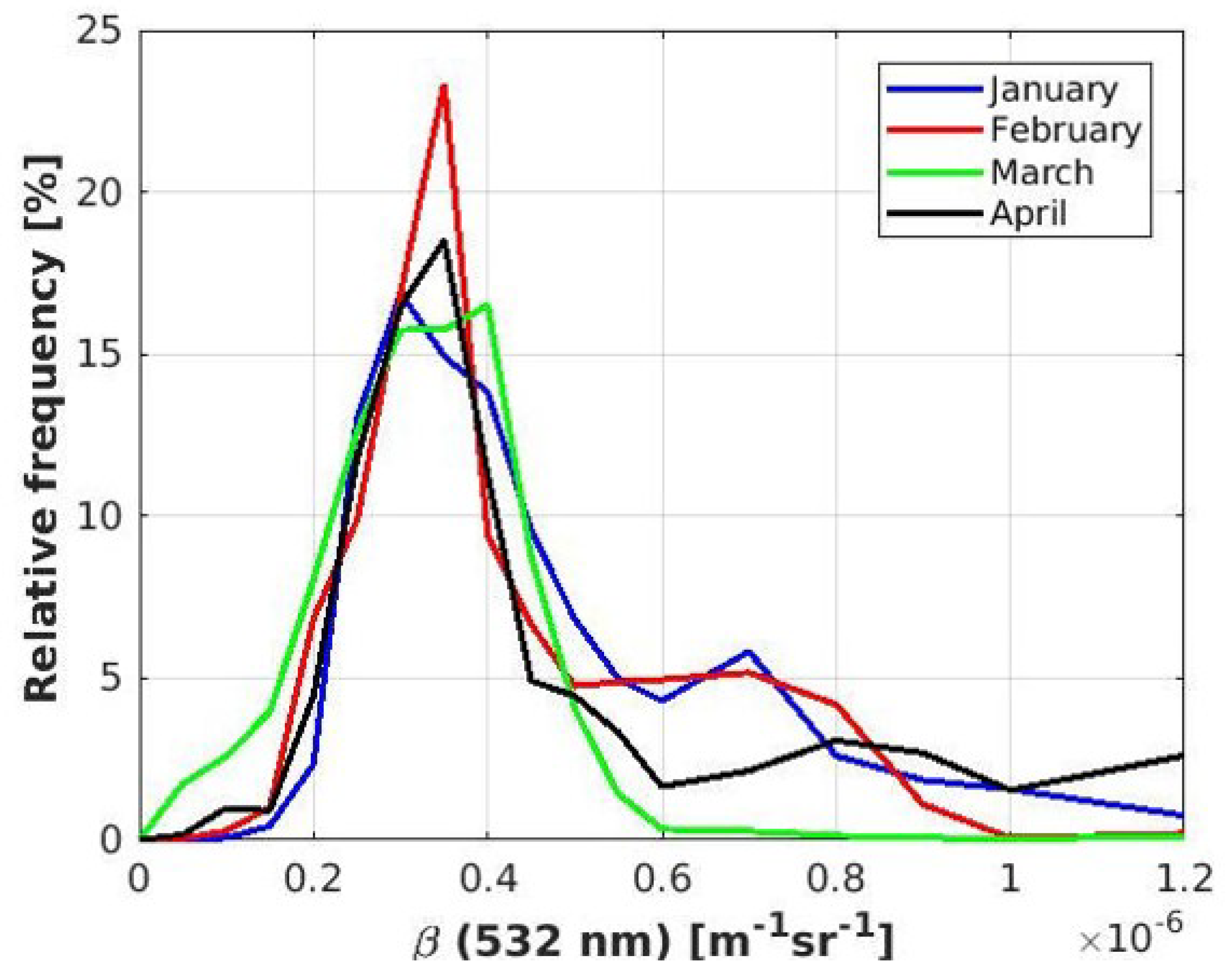
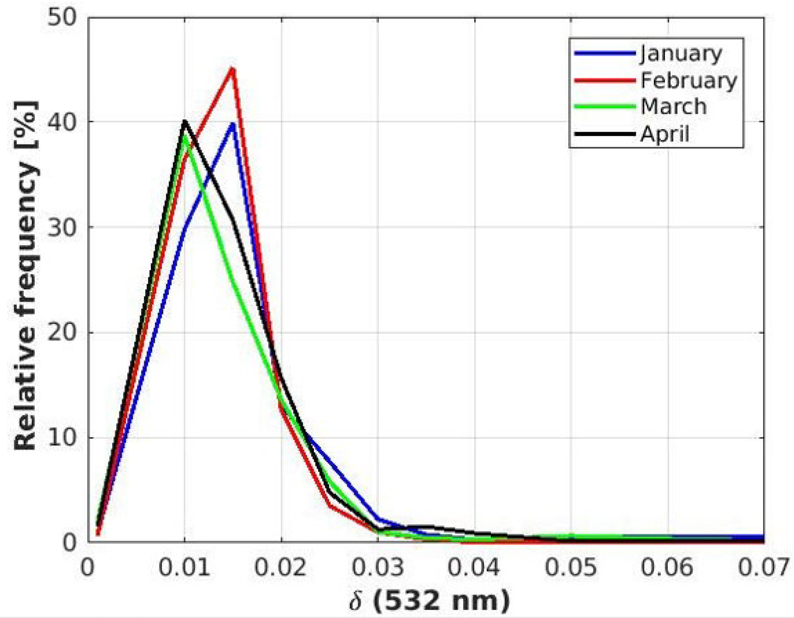
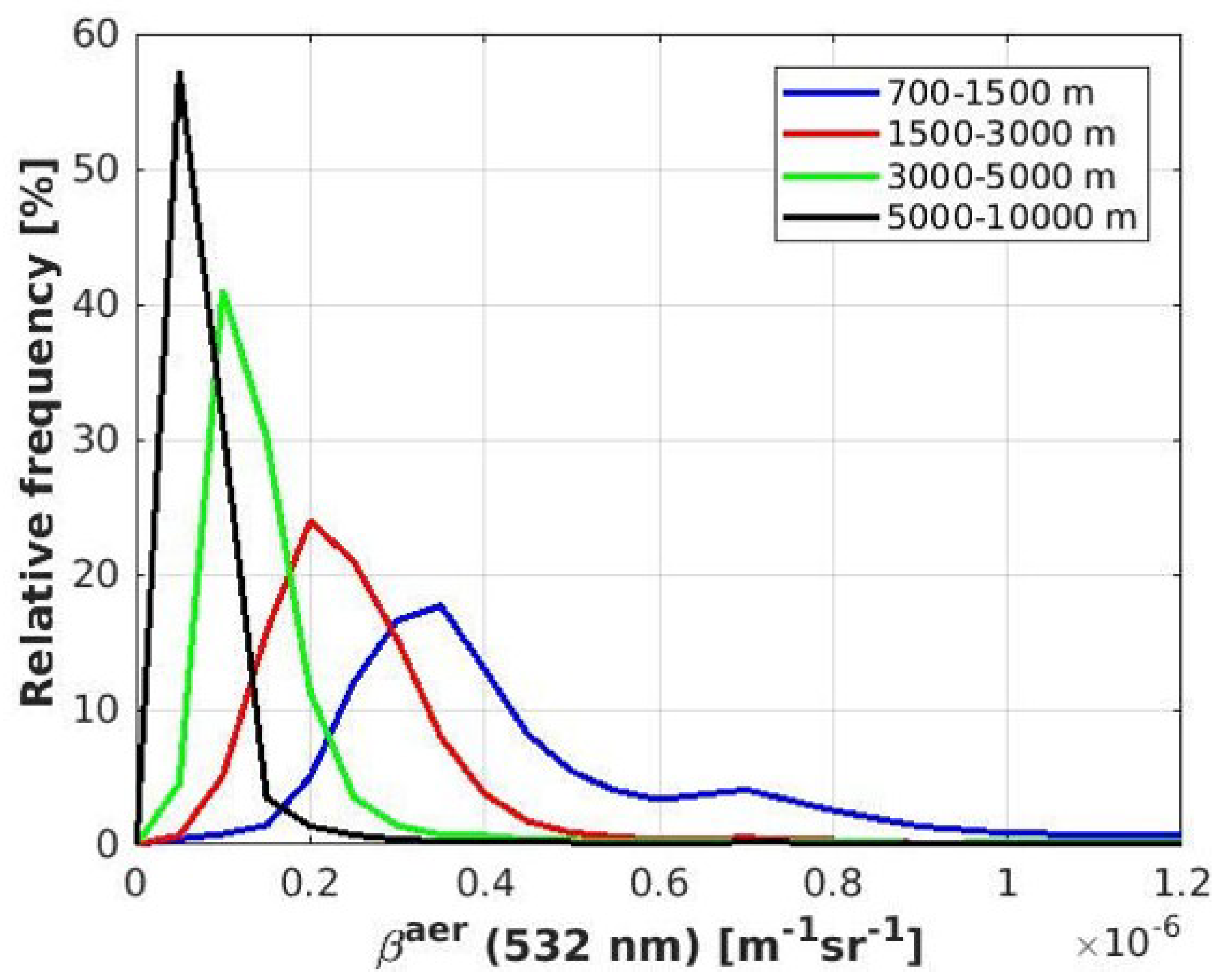
3.1. Lidar-Derived Aerosol Optical Properties in January–April 2019

In this subsection, we investigate the temporal variability of aerosol optical properties in the troposphere from January to April as well as their vertical variability. In Figure 2 and Figure 3, aerosol backscatter coefficient and aerosol depolarisation histograms are given for the height interval 700 m to 1500 m. Backscatter values above 0.6 × 10${}^{-6}$ m${}^{-1}$ sr${}^{-1}$ were hardly observed and the occurrence of increased aerosol backscatter was lower during the Arctic haze season (March, April) compared to late winter (January, February). Moreover, we did not observe any increase in the aerosol depolarisation during spring 2019. This unexpected, missing temporal variability of aerosol properties was also true for other height intervals (not shown for brevity). This indicates that the lidar-derived aerosol properties from January to April 2019 were mainly a function of altitude without pronounced temporal variability. The vertical distribution of aerosol optical properties was also analysed, with the relative frequencies of aerosol backscatter at 532 nm (Figure 4), colour ratio (Figure 5), depolarisation at 532 nm (Figure 6) and lidar ratio at 355 nm (Figure 7) displayed at four different altitude intervals.

During the whole period of late winter–early spring 2019, the highest backscatter (between 0.2 × 10${}^{-6}$ and 0.5 × 10${}^{-6}$ m${}^{-1}$ sr${}^{-1}$) was observed between 700 and 1500 m, exhibiting a large spread. This indicates higher aerosol content and variability in the lower altitudes compared to higher altitudes. Higher up in the atmosphere both the backscatter coefficient and its variability decreased.

The colour ratio showed differences between the height levels. High colour ratio values were observed between 700 and 1500 m, indicating smaller particles. However, a broadening towards lower colour ratio values was observed for 3000–5000 m and 5000–10,000 m, indicating the presence of mixed particles with different sizes and, thus different ageing state or type. The CR can reach the Rayleigh limit of ${\frac{{\lambda }_1}{\lambda 2}}^{-4}$ when very tiny aerosol is present, which was observed in clean conditions above 3 km altitude. The graphs were cut off at this limit. The depolarisation was similar for all heights, with the interval 700–1500 m displaying slightly lower depolarisation values (more spherical particles). Therefore, the aerosol microphysical properties can be inverted using Mie theory as a good approximation and subsequently the aerosol radiative impact can be estimated. The lidar ratio at 355 nm was mostly low with values around 20 sr for the heights between 700 and 5000 m. Between 700 and 1500 m, the lowest lidar ratio values were observed, indicating non-absorbing aerosol such as sea salt particles [40]. The LR between 5000 and 10,000 m was very broad, implying the presence of different aerosol types that were most likely aged and internally mixed.

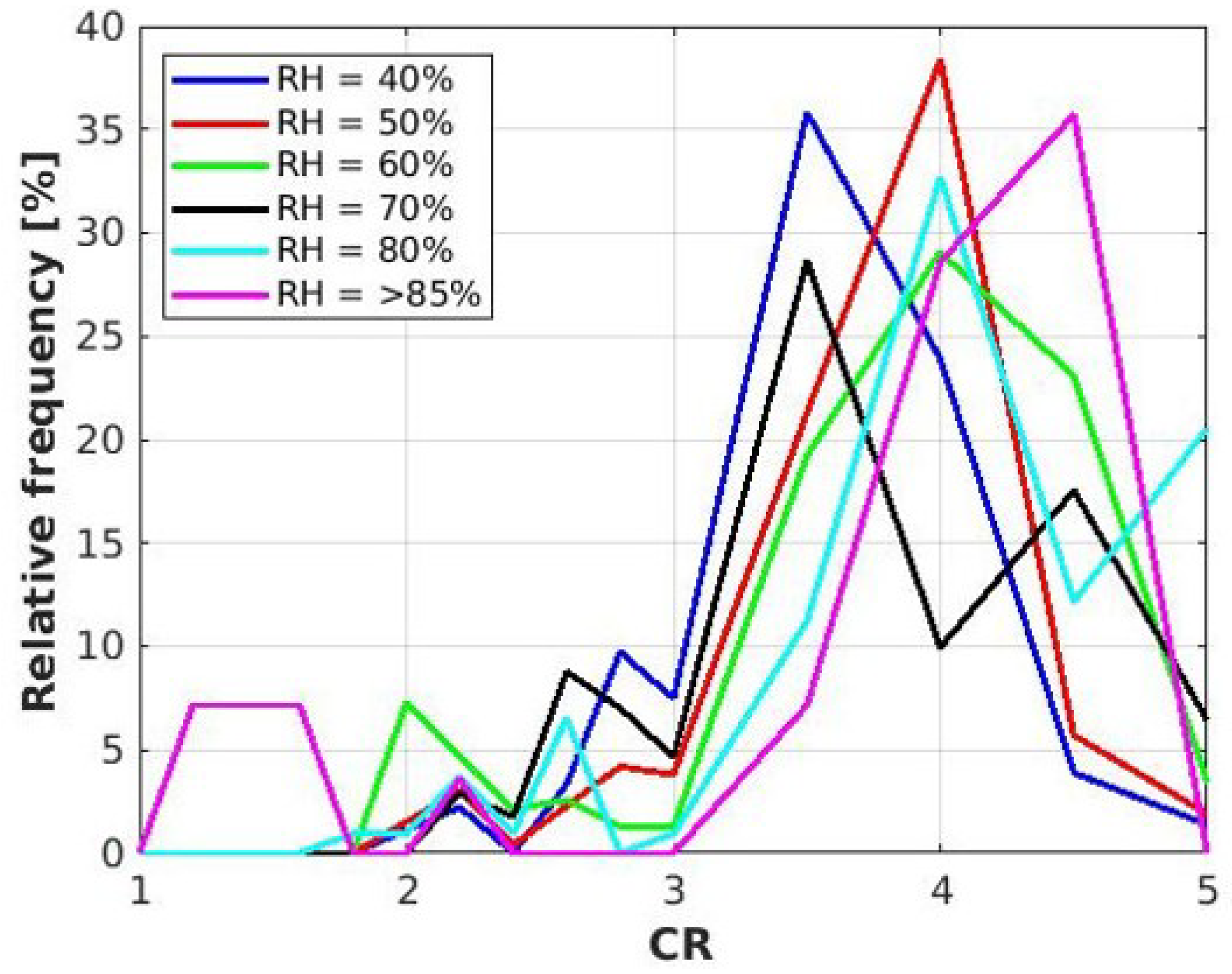
3.2. Relation between the Optical Parameters and Relative Humidity (Rh)

In the following, we investigate aerosol hygroscopicity. This is done by examining the dependence of aerosol backscatter coefficient and colour ratio on relative humidity by contemporary radiosonde data. The height interval between 1500 and 2000 m was studied in order to see a correlation between different optical parameters. Below 1500 m, the aerosol is assumed to be variable due to surrounding mountains. By contrast, above 2000 m altitude the aerosol concentrations decreases so hygroscopic effects will be harder to see. Figure 8 depicts the relation between aerosol backscatter and colour ratio. It can be seen that generally the particles are small. (A colour ratio of 2.5 in our case translates into an Ångström exponent of backscatter of 1.81, which is larger than the photometer derived Ångstöm exponent [21] for Ny-Ålesund). Larger particles are nicely correlated to larger backscatter. This means that generally the size of the aerosol determines the backscatter (not, e.g., different chemical composition).

Subsequently, the relation between aerosol backscatter and RH from contemporary (±30 min) radiosondes was analysed. In total, 22 radiosonde and 1163 matching lidar profiles were used in this comparison. In Figure 9, it can be seen that high RH did not lead to larger backscatter. Especially the profiles with highest RH (above 85%) always showed backscatter coefficients below 0.4 $\times {10}^{-6}$ m${}^{-1}{\mathrm{sr}}^{-1}$. In total, 31% of the selected observations occurred at RH < 50%. Consequently, hygroscopic effects did not play a significant role for the late winter–early spring period of 2019. According to Figure 9, the most humid parts of the atmosphere were the cleanest in terms of aerosol load. Potentially some of the hydrophilic aerosol was already washed out prior to its advection to the Arctic or, alternatively, aerosol and moisture had different origins and pathways. The same can be concluded from Figure 10. Most of the aerosol found at RH > 85% had a colour ratio larger than 4, with this corresponding to very small particles. Only a few cases (~21.4%, in

Table A2. Relative frequencies of the colour ratio between 1500 and 2000 m for different RH values.

CR Classes	RH = 40%	RH = 50%	RH = 60%	RH = 70%	RH = 80%	RH > 85%
1.0001	0.00	0.00	0.00	0.00	0.00	0.00
1.2	0.00	0.00	0.00	0.00	0.00	7.14
1.4	0.00	0.00	0.00	0.00	0.00	7.14
1.6	0.00	0.00	0.00	0.00	0.00	7.14
1.8	0.00	0.00	0.00	0.00	0.93	0.00
2	1.11	1.52	7.26	0.00	0.93	0.00
2.2	2.22	3.04	4.70	2.92	3.74	3.57
2.4	0.00	0.38	2.14	1.75	0.93	0.00
2.6	3.33	2.28	2.56	8.77	6.54	0.00
2.8	9.72	4.18	1.28	7.02	0.00	0.00
3	7.50	3.80	1.28	4.68	0.93	0.00
3.5	35.83	21.29	19.23	28.65	11.21	7.14
4	23.89	38.40	29.06	9.94	32.71	28.57
4.5	3.89	5.70	23.08	17.54	12.15	35.71
5	1.39	1.90	3.42	6.43	20.56	0.00
sum	87.50	80.61	90.60	81.29	70.09	96.43
No. of data points	360	263	234	171	107	28

) and under very high RH conditions (RH > 85%) showed a colour ratio smaller than 2, indicative of hygroscopic growth. Detailed numbers belonging to Figure 9 and Figure 10 are shown in

Table A1. Relative frequencies the aerosol backscatter at 532 nm between 1500 and 2000 m for different RH values.

Beta Classes	RH = 40%	RH = 50%	RH = 60%	RH = 70%	RH = 80%	RH > 85%
1 × ${10}^{-9}$	0.28	0.38	0.00	0.00	0.00	0.00
5 × ${10}^{-8}$	2.50	4.18	1.71	3.51	0.00	0.00
1 × ${10}^{-7}$	0.00	0.38	1.71	0.00	2.80	0.00
1.5 × ${10}^{-7}$	1.39	1.14	4.70	4.68	18.69	0.00
2 × ${10}^{-7}$	20.56	23.57	46.15	8.77	11.21	46.43
2.5 × ${10}^{-7}$	11.67	33.08	20.09	27.49	6.54	17.86
3 × ${10}^{-7}$	24.72	8.37	10.68	18.71	21.50	7.14
3.5 × ${10}^{-7}$	16.94	4.94	3.42	19.88	32.71	0.00
4 × ${10}^{-7}$	6.39	11.03	10.26	13.45	2.80	0.00
4.5 × ${10}^{-7}$	6.39	0.76	0.85	1.17	1.87	0.00
5 × ${10}^{-7}$	0.83	0.00	0.00	1.75	0.00	0.00
5.5 × ${10}^{-7}$	0.00	0.00	0.43	0.00	0.00	0.00
6 × ${10}^{-7}$	0.00	0.00	0.00	0.58	0.00	0.00
7 × ${10}^{-7}$	0.00	0.00	0.00	0.00	0.00	0.00
8 × ${10}^{-7}$	0.00	0.00	0.00	0.00	0.93	0.00
9 × ${10}^{-7}$	0.00	0.00	0.00	0.00	0.93	0.00
1 × ${10}^{-6}$	0.00	0.00	0.00	0.00	0.00	0.00
1 × ${10}^{-6}$	0.00	0.00	0.00	0.00	0.00	0.00
sum	91.67	87.83	100.00	100.00	100.00	71.43
No. of data points	360	263	234	171	107	28

and Table A2 in Appendix A.

3.3. In-Situ Measurements during Spring 2019

Figure 11 shows nss-SO${}_4^{2-}$ concentration trends in aerosol samples collected at Gruvebadet and Zeppelin Observatories in the period January–June 2019 at daily–two day resolution. nss-SO${}_4^{2-}$ is one of the main components of the Arctic haze and has been widely used as a proxy of this process in the high Arctic since many decades (e.g., Sharma [15] and Udisti [42]). Their concentration trends usually show a clear increase during the Arctic haze months peaking in March and/or April [12,16,38] and they have been used also to define the timing and characterise the Haze along the years. In 2019, surprisingly nss-SO${}_4^{2-}$ does not show such a clear-cut signature, with a large occurrence of relatively high peaks from January to May. This pattern can be observed both at Gruvebadet and Zeppelin although the latter exhibits a lower variability (0.509 ± 0.500 $\mathsf{\mu }$g m${}^{-3}$ and 0.477 ± 0.413 $\mathsf{\mu }$g m${}^{-3}$). In order to better appreciate the possible seasonal changes, distribution plots are reported in Figure 12 and Figure 13. Despite a waving pattern in median values at Gruvebadet (ranging between 0.310 and 0.695 $\mathsf{\mu }$g m${}^{-3}$), half of the values (box amplitude) spans a broad but comparable range between January and May (between 0.15 and 1.0 $\mathsf{\mu }$g m${}^{-3}$), to drop more clearly only in June (0.10–0.25 $\mathsf{\mu }$g m${}^{-3}$. At Zeppelin this sort of “steady-state” pattern during the Haze months is even clearer, with very close median values from January to May (0.20–0.48 $\mathsf{\mu }$g m${}^{-3}$) and especially very similar data distribution, which shows again lower values only in June.

The peculiar features of 2019 Arctic haze can be observed also in Figure 14, showing the source apportionment of sulphate accomplished for Gruvebadet on the basis of ion ratios in sea salt, crustal and biogenic sources [16]. It can be seen that anthropogenic sulphate covers most of the budget of nss-SO${}_4^{2-}$ (include also biogenic and crustal sulphate) in the whole period from January to May, except for a few days in mid May, where biogenic source accounts for at least half of sulphate concentration, as expected for this time of the year [44]. Starting from early June, anthropogenic sulphate drops while biogenic and sea salt inputs become more important. As anthropogenic sulphate can be related to the Arctic haze and/or other long-range transport processes, it appears that either the Haze has surprisingly lasted all through May or different processes (for instance, local meteorology) are taking place and controlling sulphate concentration so that no “classical Arctic Haze period” can be actually detected in this year at Ny-Ålesund. In the latter case, we should probably revise the classical definition of Arctic haze, especially if such a pattern will be observed in the upcoming years.

4. Discussion

4.1. Comparing Lidar Data 2019 with 2018 and 2014

In order to assess the variability of Arctic haze on longer time scales, we compared the findings of this study (season of 2019) with the aerosol conditions during the years 2018 and 2014.

Müller [45] evaluated Lidar data from 1st of March to 13th of March 2018 over the site of Ny-Ålesund. That data were used to compare with all available March 2019 data (5, 7, 21–23, 25–28 and 30–31 of March). Figure 15, Figure 16 and Figure 17 show the comparison for the backscatter, the colour ratio and depolarisation ratio (see

Table A3. Aerosol backscatter data from 1 to 13 March 2018 (Müller [45]) in comparison to the data from this study (all available data from March 2019). The first value in each cell (in italic) represent the 2018 data, while the second value represents the 2019 (this study). Note the fact that the values of this study do not sum up as 100%: this is because the data were filtered for clouds and those values have been left out in the table and graphs, but have been included while calculating the relative frequencies.

$\mathsf{\beta }$ (532 nm) (10${}^{-6}$ m${}^{-1}$ sr${}^{-1}$)	700–1500 m	1500–3000 m	3000–5000 m	5000–10,000 m
0–0.1	4.30 4.38	5.09 7.05	11.29 30.16	83.39 86.43
0.1–0.2	0.96 12.02	11.11 42.12	67.28 50.85	8.27 7.50
0.2–0.3	28.31 28.36	65.42 34.93	18.30 7.44	2.33 1.09
0.3–0.4	37.27 32.27	12.04 8.97	0.70 2.47	1.23 0.46
0.4–0.5	14.17 12.82	1.46 0.62	0.30 1.32	0.82 0.39
0.5–0.6	14.98 1.76	4.88 0.48	1.58 0.68	3.96 0.22

,

Table A4. Comparing the depolarisation ratios of Müller (2018) of the 1–13 March 2018 with the data from this study, considering all available data for March 2019. The first value in each cell (in italic) represent the data of Müller (2018), the second value represents the data found in this study. The ranges of the second and third differed slightly in the study of Müller compared to this study.

Range	700–1500 m	1500–3000 m	3000–5000 m	5000–10,000 m
0–1.0	50.25 40.80	33.83 8.19	8.30 11.45	5.76 15.07
1.0–1.4 1.0–1.5	42.48 24.81	54.55 33.73	30.28 28.03	9.12 27.49
1.4–2.0 1.5–2.0	2.05 13.62	6.00 27.75	39.58 26.95	17.83 26.84
2.0–2.5	0.96 5.83	0.58 13.03	14.08 11.91	22.79 13.47
2.5–3.0	0.63 1.05	0.58 3.68	4.67 6.13	20.57 5.87
3.0–3.5	0.91 0.47	0.33 1.65	0.54 2.86	10.78 2.78
3.5–4.0	0.58 0.31	0.24 0.92	0.07 1.33	4.13 1.38
4.0–5.0	0.10 0.66	0.61 1.31	0.26 1.68	3.51 1.37

and

Table A5. Comparing the CR values of Müller (2018) of the 1–13 March 2018 with the data from this study, considering all available data for March 2019. The first value in each cell (in italic) represents the data of Müller (2018), the second value represents the data found in this study. Note the fact that the values of this study do not sum up as 100%: this is because the data were filtered for clouds and those values have been left out, but have been included while calculating the relative frequencies.

CR	700–1500 m	1500–3000 m
1–2	10.64 6.46	3.75 4.67
2–3	15.44 44.98	7.75 19.31
3–4	30.66 24.06	26.98 32.26
4–5	41.92 7.04	60.65 18.32

in the Appendix B).

Between 700 and 5000 m altitude, higher aerosol backscatter coefficient values were observed in 2018. The largest differences were found for the height interval between 1500 m to 3000 m altitude. Above 5000 m the atmosphere was very clear in both years, as low backscatter with almost identical backscatter frequency distributions was observed. The depolarisation was generally low and indicates almost spherical particles. Slightly lower depolarisation values were found below 5000 m for 2018. Above that altitude the conditions changed and the depolarisation was larger in 2019. Therefore, the 2019 data suggest a depolarisation which rises with altitude while in 2018 this trend is far less obvious. The colour ratio between 700 and 1500 m seemed to be more uniform in 2019 and showed a broader distribution with a tail of small particles in 2018. Between 1500 and 3000 m the particles were larger (lower CR) during 2019, despite the lower backscatter.

The lidar data of 2019 were also briefly compared to those derived during the iAREA campaign in April 2014. During the iAREA campaign the aerosol backscatter coefficient was mostly around 0.4 ×10 ${}^{-6}$ m${}^{-1}{\mathrm{sr}}^{-1}$ (1000–1500 m). This is similar to April 2019, as a peak around 0.4 $\times {10}^{-6}$ m${}^{-1}{\mathrm{sr}}^{-1}$ was observed as well (700–1500 m). The depolarisation ratio in April 2014 peaked between 0.02 and 0.03 (1000–1500 m). In April 2019, the depolarisation ratio was mostly 0.01–0.02 (700–1500 m). Therefore, the aerosol backscatter coefficient patterns of April 2019 were similar to those of the iAREA campaign. However, in this study the depolarisation ratio was slightly lower, indicating more spherical particles.

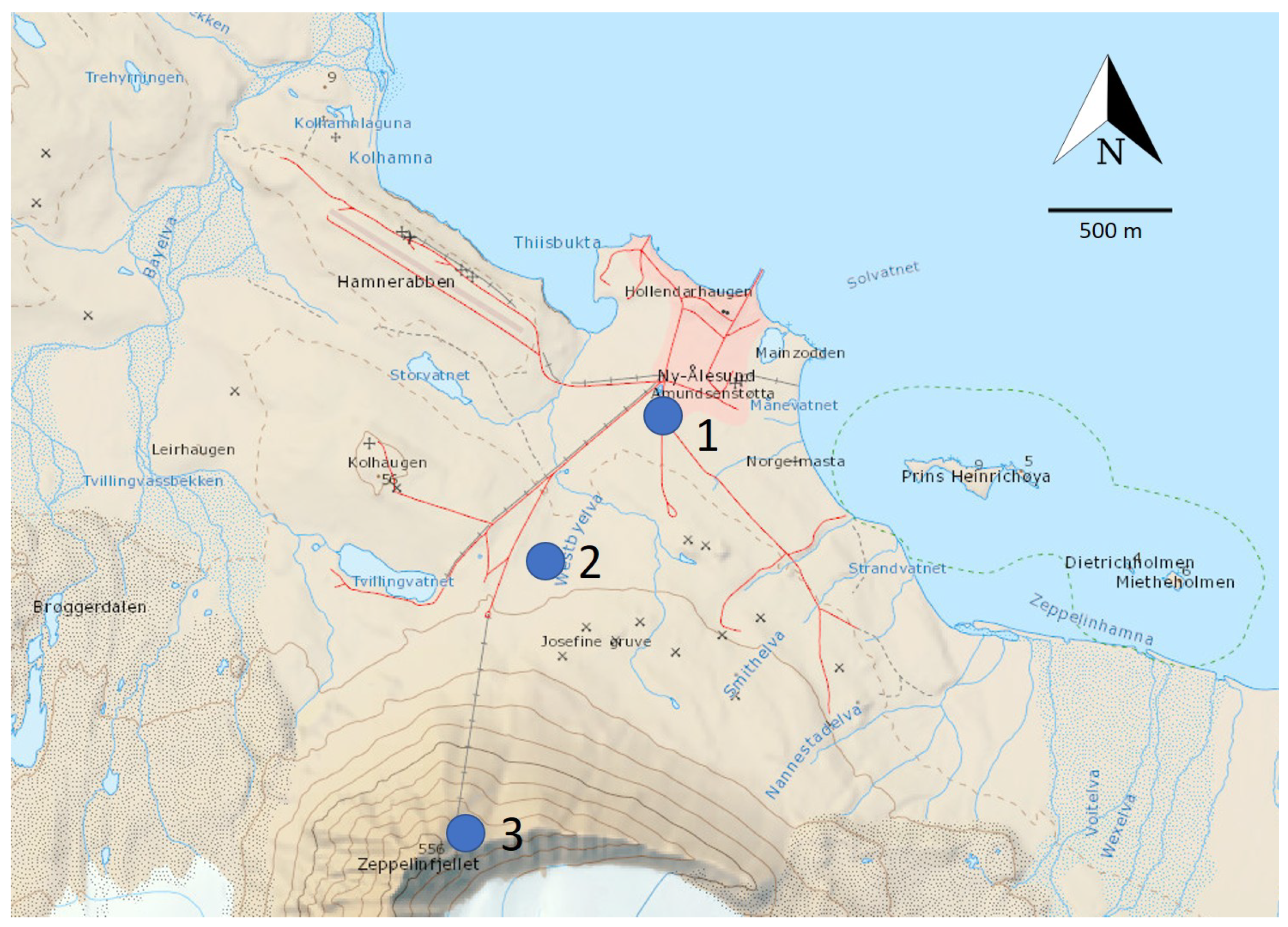
4.2. Comparing Different Sites around Ny-Ålesund

As an Arctic site, Ny-Ålesund typically faces a shallow and stable boundary layer in winter and early spring [31,46]. In reality, the boundary layer structure might be complicated due the orographically structured terrain of Ny-Ålesund that causes pronounced micrometeorology [31]. For this reason, we investigated the evolution of the boundary layer height on a daily basis. In Figure 18, the boundary layer height is shown for late winter and early spring 2019, as derived by the bulk Richardson number (using the local radiosounding data). The bulk Richardson number [47] considers profiles of potential temperature and wind and is a well suited criterion to determine the boundary layer height even under thermally stable conditions. The boundary layer during late winter–early spring 2019 was always shallower than 200 m, and especially low from January to March. In the majority of the study period (66%), the boundary layer top height was below 100 m, with a median height of 70 m. The low Arctic boundary layer height clearly indicates that the lidar provides measurements (starting at 700 m altitude) above the local boundary layer and, thus, the reconciliation with ground-based in situ observations is not a straightforward task. There might even be different aerosol compositions between the Gruvebadet and Zeppelin site with less local, marine aerosol being present at the latter station.

Figure 19 presents the correlation between the in situ measured nss-SO${}_4^{2-}$ at the Zeppelin (mountain) and Gruvebadet stations. The same data as for Figure 11 are shown. Despite the low boundary layer height the correlation of nss-SO${}_4^{2-}$ is almost 0.7 ($R^2$ = 0.48) and, considering the large data set (more than 100 values), it is highly significant (>99%). Furthermore, no systematic bias between the two sites can be seen (the linear fit slope is close to one). Therefore, neither of the stations systematically missed a fraction of the aerosol. However, as the nss-SO${}_4^{2-}$ is expected to be long-range transported (there are hardly any local sources), the differences at the two in situ stations are remarkable. Our observations support the following mechanism: in late winter–early spring aerosol is advected into the Arctic in the lower free troposphere (higher wind speed and less vertical mixing compared to the ground). As reported by Thomas et al. [48], aerosol in the Arctic is mainly advected in lower altitudes during winter, while stronger boundary layer stability results in increased aerosol trapping below inversions. However, whether the aerosol will be finally collected by the ground-based in situ instruments depends on the downward vertical mixing, and therefore on the boundary layer stability. Therefore, the role of downward vertical mixing as a linking parameter between boundary layer and free tropospheric aerosol conditions are probably important in the Arctic.

While nss-SO${}_4^{2-}$ is thought to be the most important component of Arctic haze [12,49], it will not be the only component on an Atlantic coastal site in years with below average pollution [16]. To estimate the importance of nss-SO${}_4^{2-}$ during the winter–spring season 2019, the relation between PM10 and nss-SO${}_4^{2-}$ is plotted in Figure 20 and Figure 21. It can be seen that the correlation is not very high, especially for higher PM10 concentration the correlation gets poor.

The aerosol backscatter at 1–2.5 km exhibited less variability (correlation among the backscatter in the three layers of Figure 22 larger than 0.6) as qualitatively compared to the sulphate concentration (Figure 11). Even though both the ground-based and mountain Zeppelin stations revealed sharp sulphate concentration peaks between end of March and beginning of April (Figure 11), the lidar did not detect any aerosol backscatter peak despite its higher temporal and vertical resolution. Further, we note from the missing correlation between lidar data and surface nss-SO${}_4^{2-}$ that even in the altitude of the lidar measurements sulfate is probably still not the dominant aerosol component in our data.

In conclusion, although the backscatter coefficient between 700 and 1500 m varied only by a factor of 3 (Figure 4, Table A3) the concentration of the main in situ aerosol species fluctuated by a factor of 25 (Figure 11). Therefore, we hypothesise that the fraction of long-range transported aerosol measured on ground was heavily influenced by boundary layer dynamics such as downward vertical mixing. This effect is expected to be more pronounced in sites with heterogeneous orography as Ny-Ålesund. By contrast, in the free troposphere the aerosol properties mainly become a function of large scale advection and synoptic meteorological conditions. Considering that the transport of nss-SO${}_4^{2-}$ from mid-latitudes into the Arctic takes about one week in winter [50], rapid changes in aerosol properties, in the order of hours, are only expected under highly variable meteorological conditions such as changing wind direction. For the aforementioned reasons, the aerosol properties should exhibit lower temporal variability in the free troposphere compared to the ground, as observed in this study. If this were true, boundary layer dynamics would play a key role for the analysis of ground-based aerosol properties at remote locations at least for the European Arctic. Likewise, Thomas et al. [48] highlighted that vertical aerosol distribution depends on the strength of temperature inversions.

5. Conclusions and Outlook

In this study, we analysed lidar-derived aerosol observations in combination with in situ non-sea salt sulfate measurements. Our investigation focused on the remarkably aerosol clear period of late winter–early spring 2019. As the measurements were obtained from three different sites—Ny-Ålesund (lidar), Gruvebadet and Zeppelin (in situ)—embedded in complex orography, we placed special emphasis on their reconciliation feasibility. The main findings of this study can be summarised as follows:

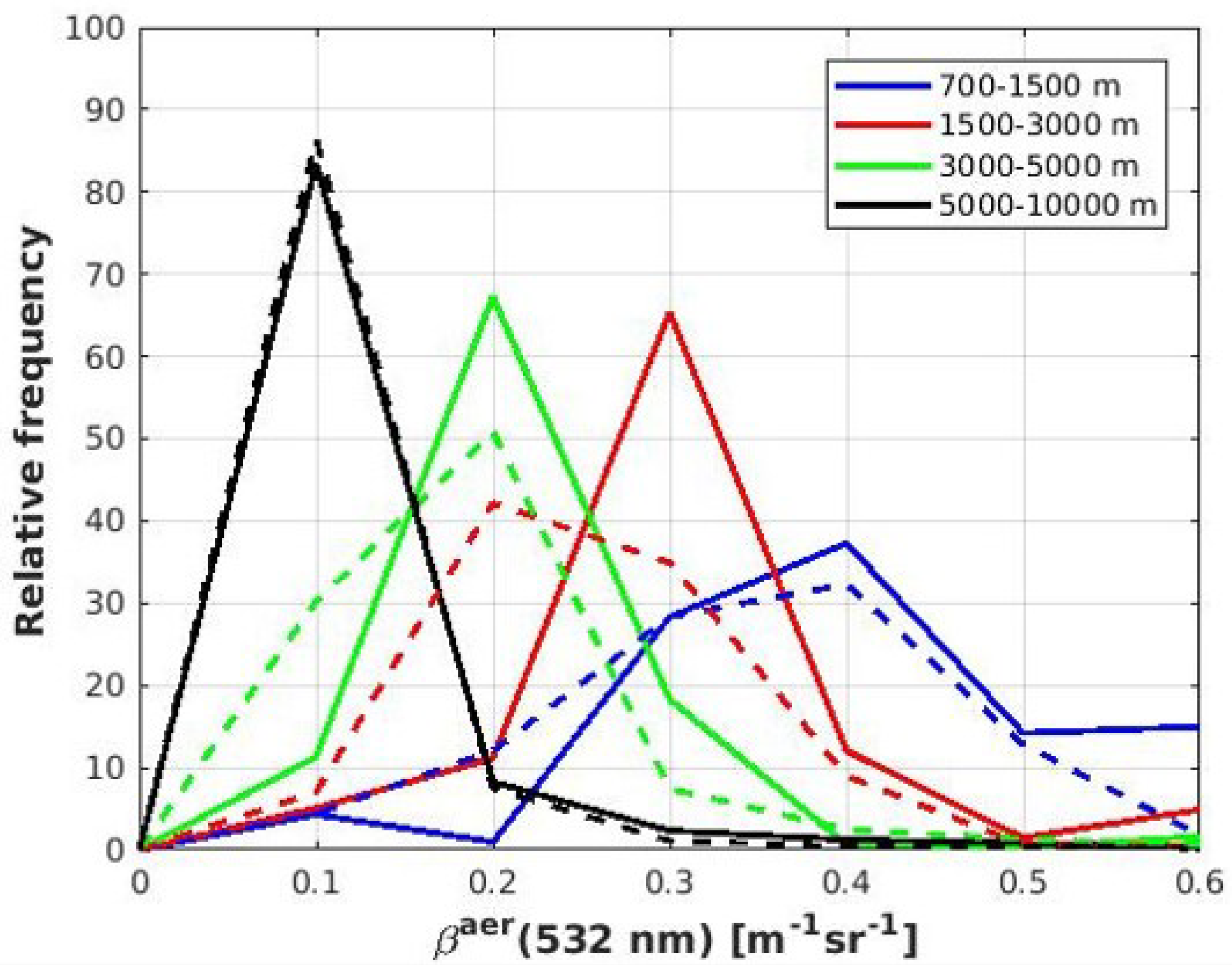
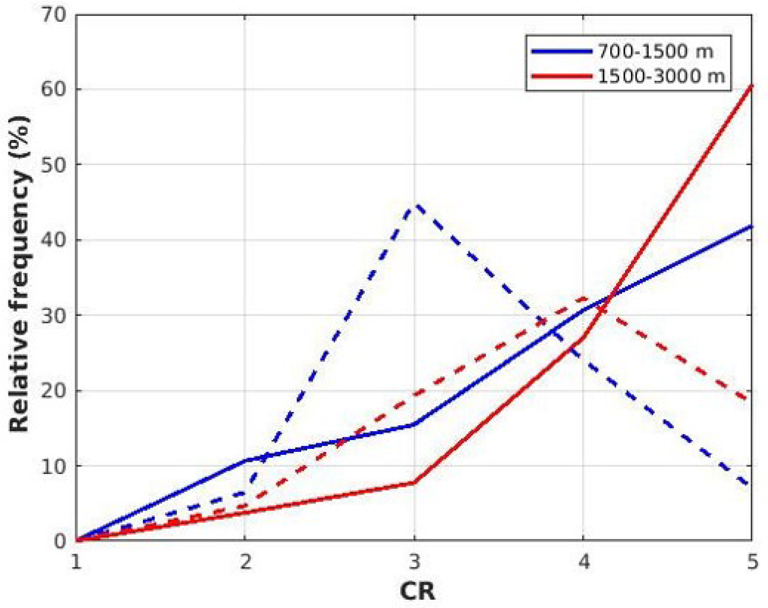
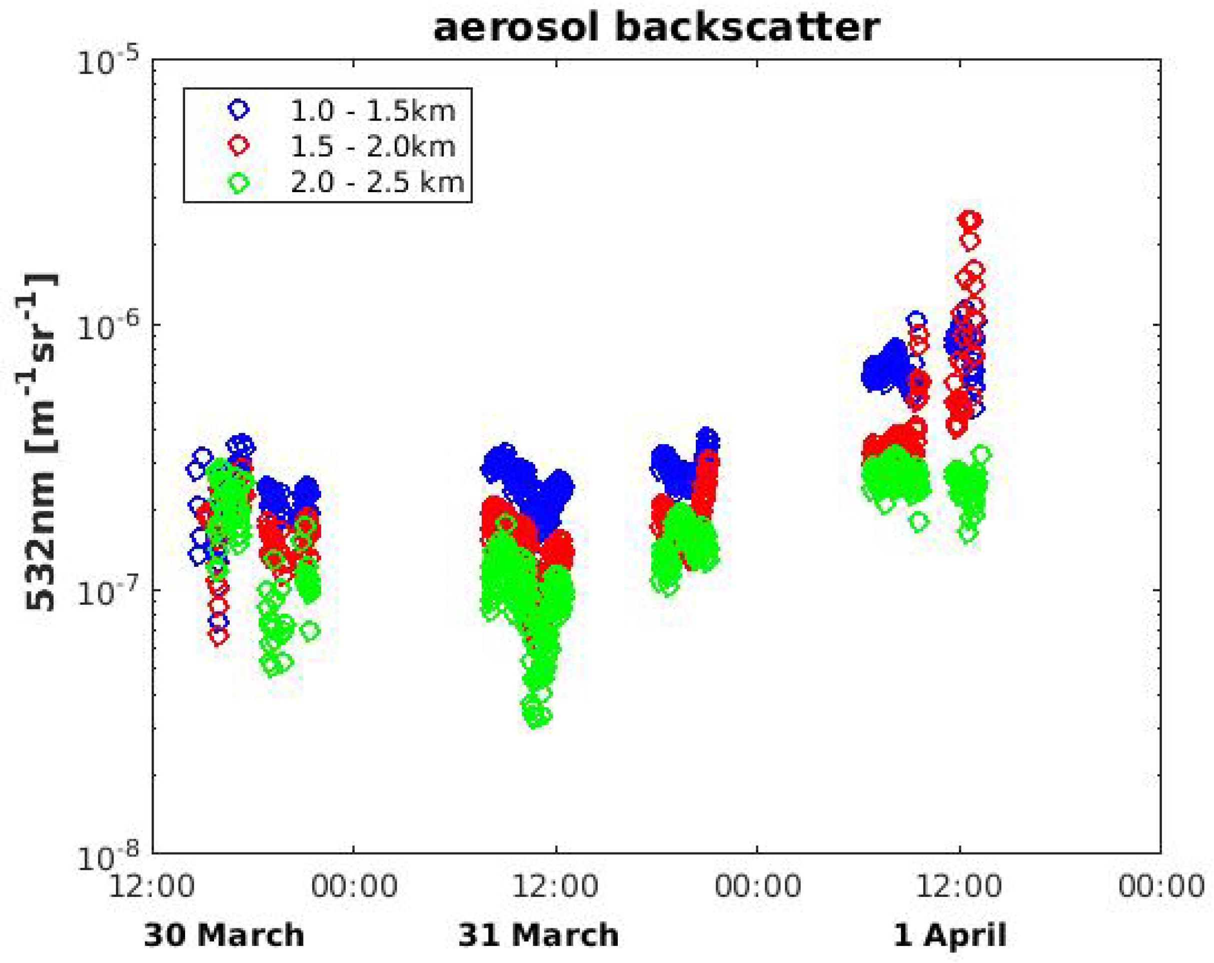
• The late winter–early spring season of 2019 was clear, with lower aerosol backscatter coefficient, especially in the altitude from 1.5 km to 3 km and lower non-sea salt sulphate concentration compared to previous years [13,14,27,51]. In contrast to other years, the aerosol backscatter in the free troposphere did not increase during March and April, the otherwise peak months for Arctic Haze. Therefore, for the European Arctic site of Ny-Ålesund and from the lidar perspective, 2019 presented itself “as a year without obvious Arctic Haze”. In the future, our findings can be compared with satellite lidar or ground-based observations from the American and Russian parts of the Arctic. Such a comparison could be used to answer the question, whether the (remaining) Arctic Haze phenomenon is mainly governed by the sources (decrease depending on source region) or sinks of aerosol (dependent on local meteorological conditions).
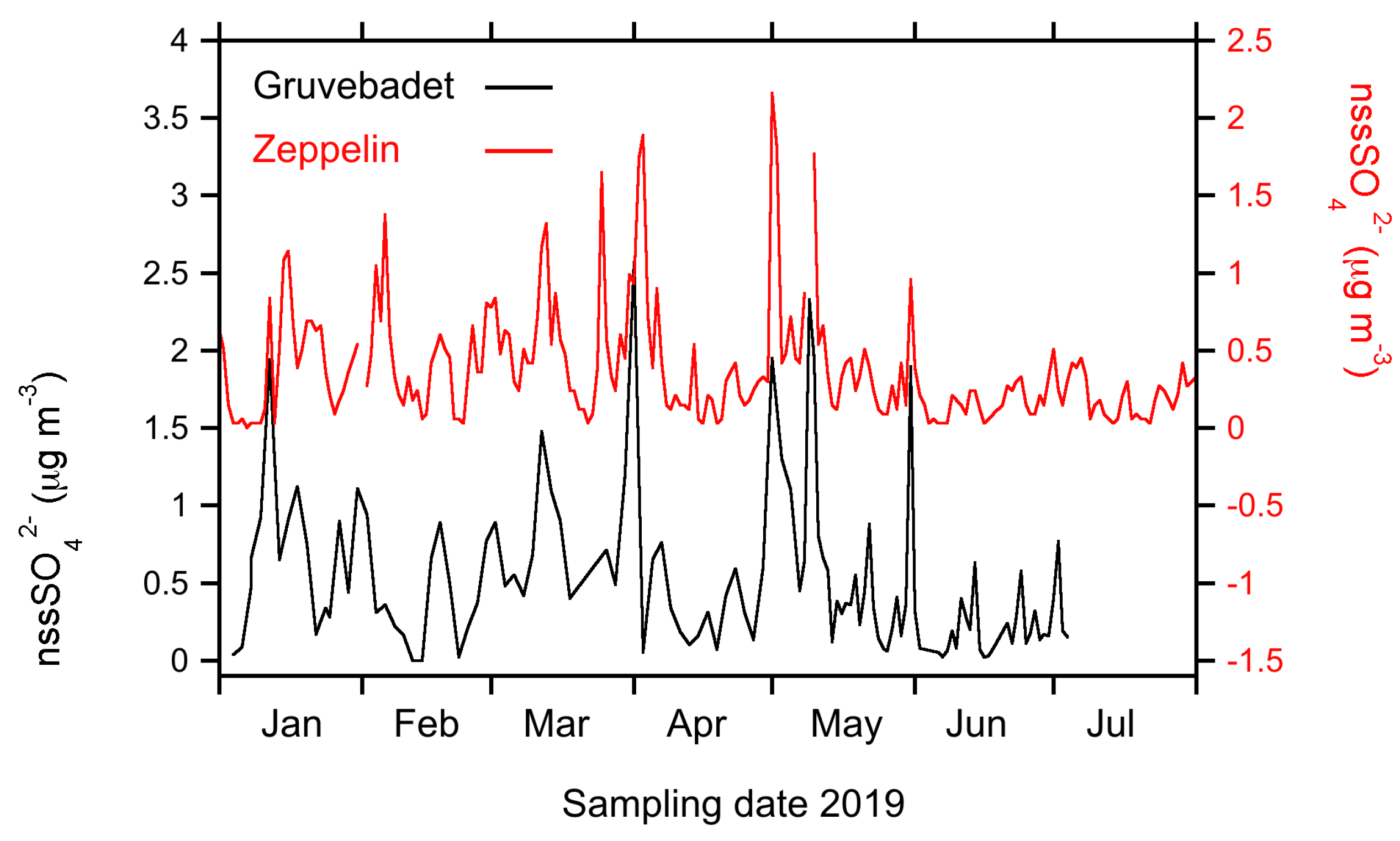
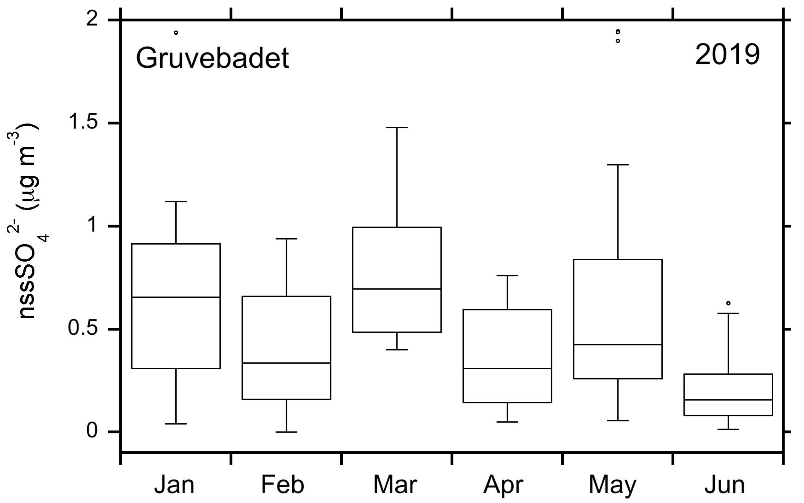
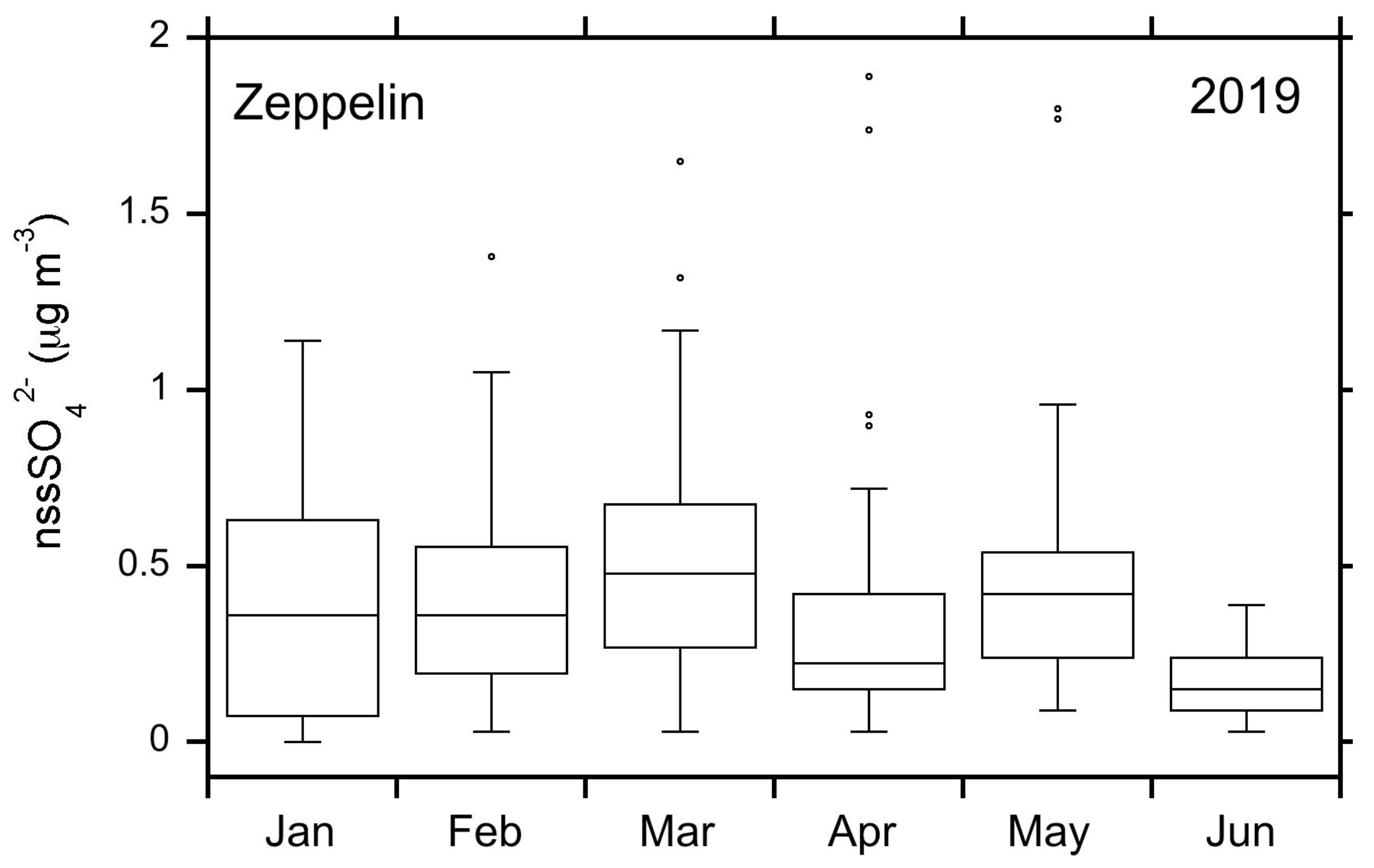
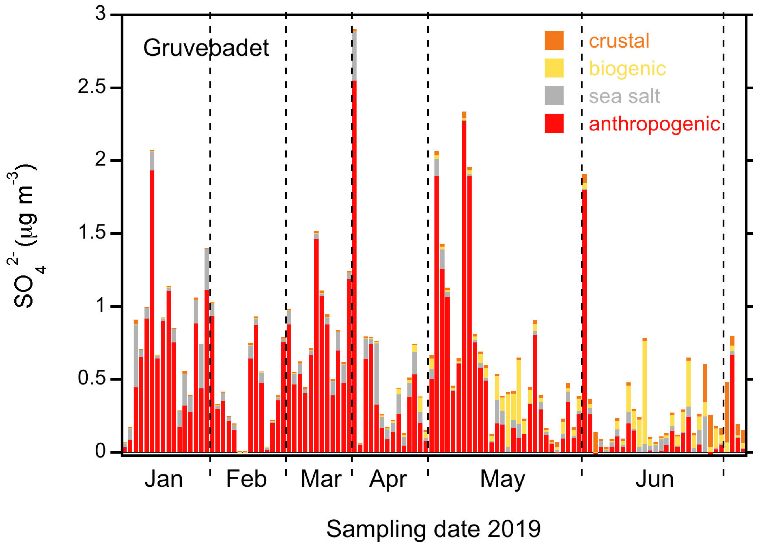
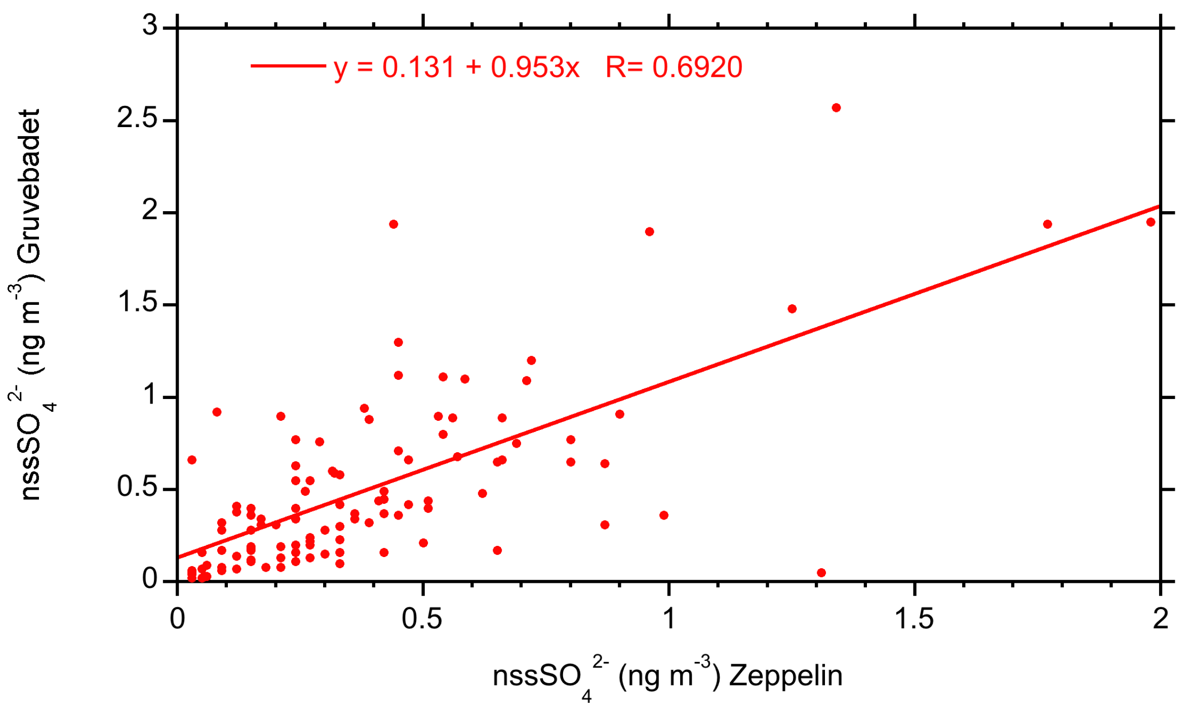
• In situ measurements from the two nearby stations, on mountain Zeppelin and at Gruvebadet (sea level), compared well for long-range advected sulphate on a seasonal basis (slope close to one). However, daily nss-sulphate concentration only showed a correlation in the order of 0.7. Moreover, we expect differences in aerosol composition between the two in situ sites, with less local marine aerosol at Zeppelin station. Therefore, a combined assessment of aerosol chemical composition at the Gruvebadet and Zeppelin sites is needed in the future.
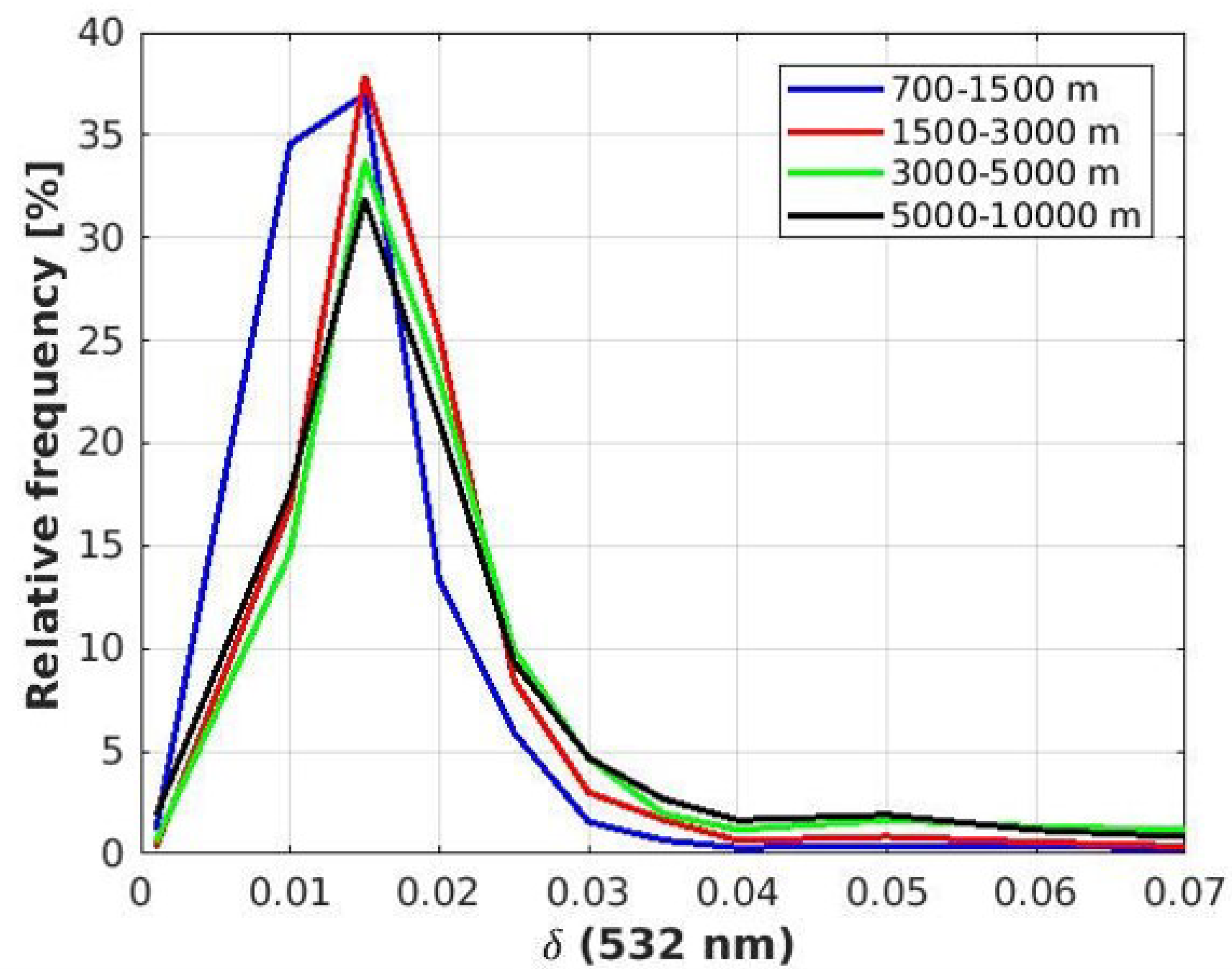
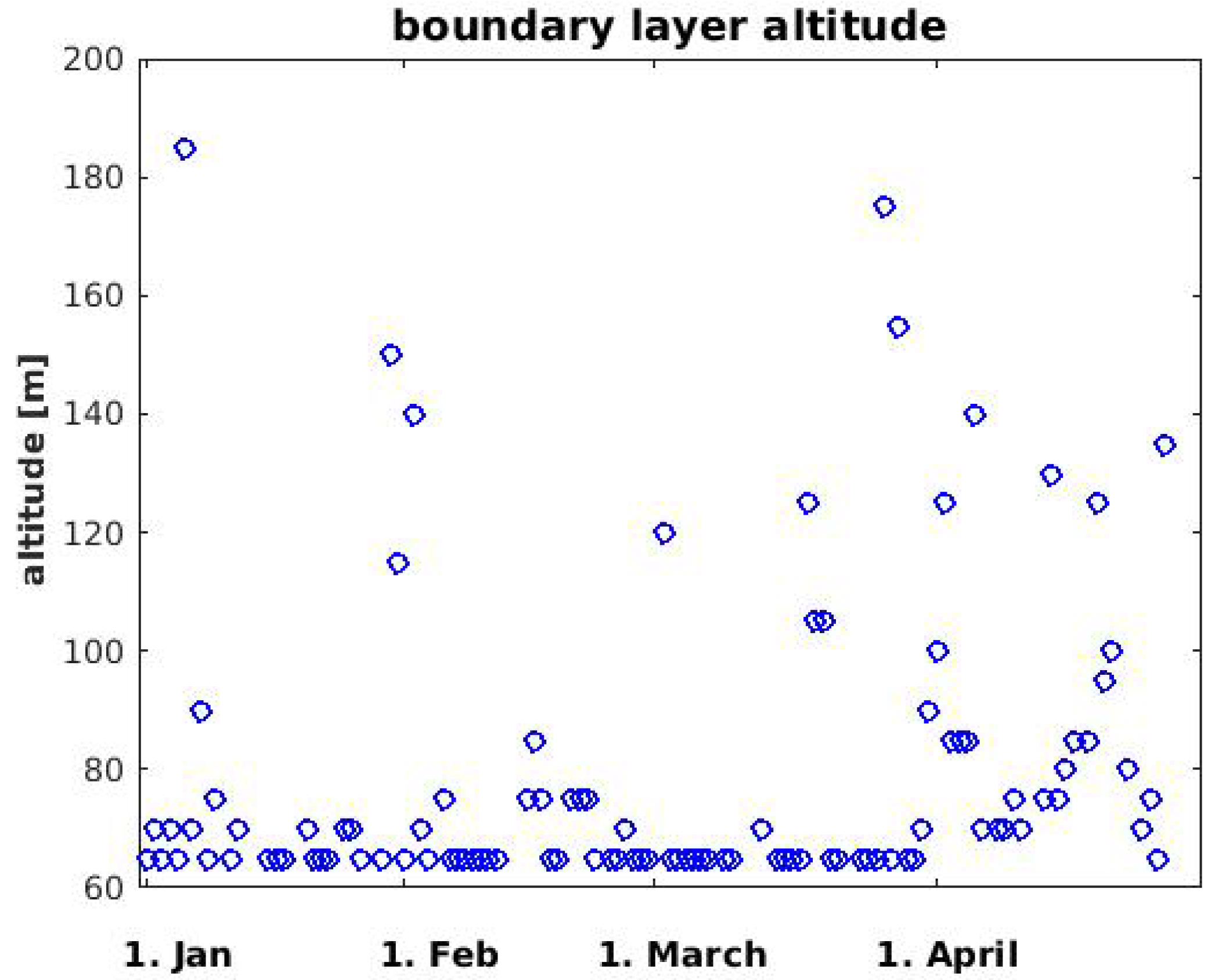
• Over Ny-Ålesund, the aerosol load changed by less than a factor of 3.5 above 700 m. Surprisingly, the daily sampled nss-sulphate concentration erratically changed by a factor of 25 (from 0.1 to 2.5 ng m${}^{-3}$) both at Gruvebadet (ground level) and Zeppelin station (474 m a.s.l.), with the latter mostly lying above the boundary layer during the study period. Overall, spherical particles were observed by the lidar. In the higher troposphere, the aerosol backscatter coefficient was confined to low values, indicating longer temporal scales and less mixing with new air masses.
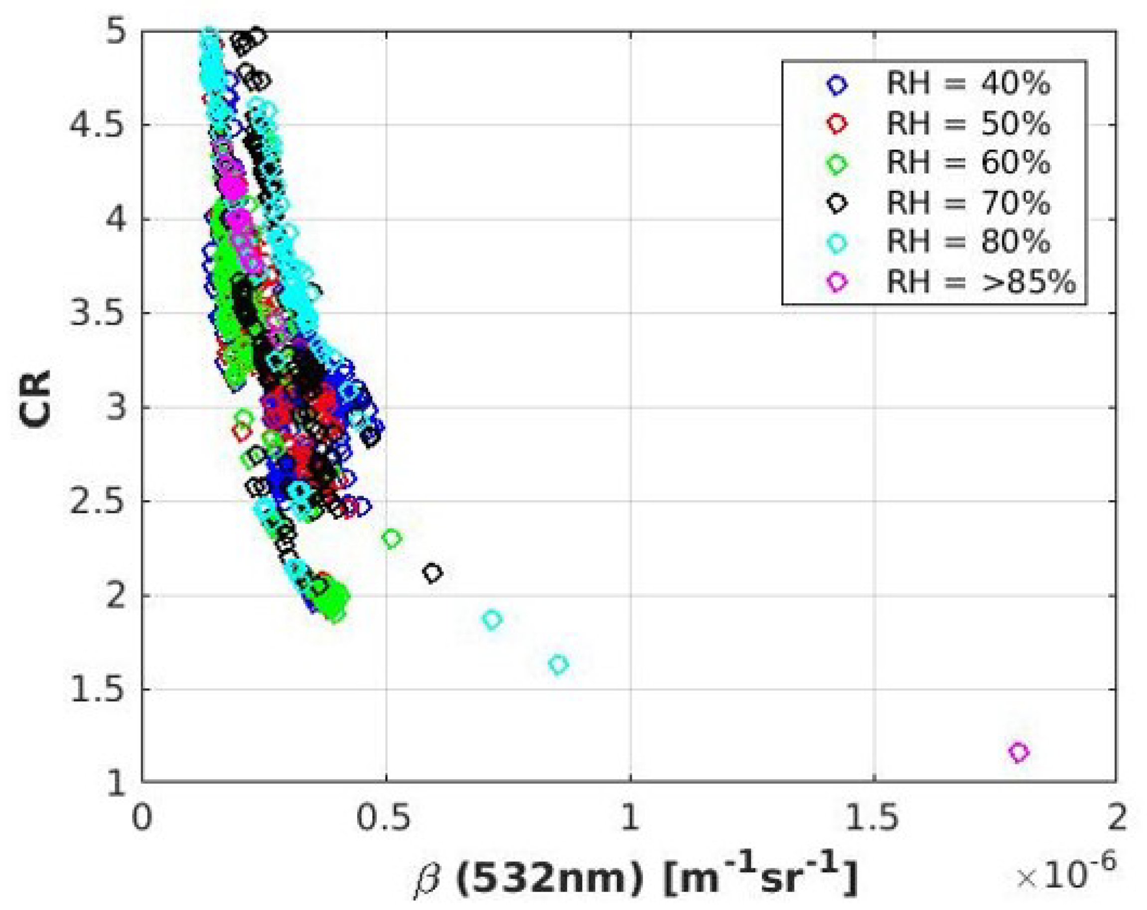
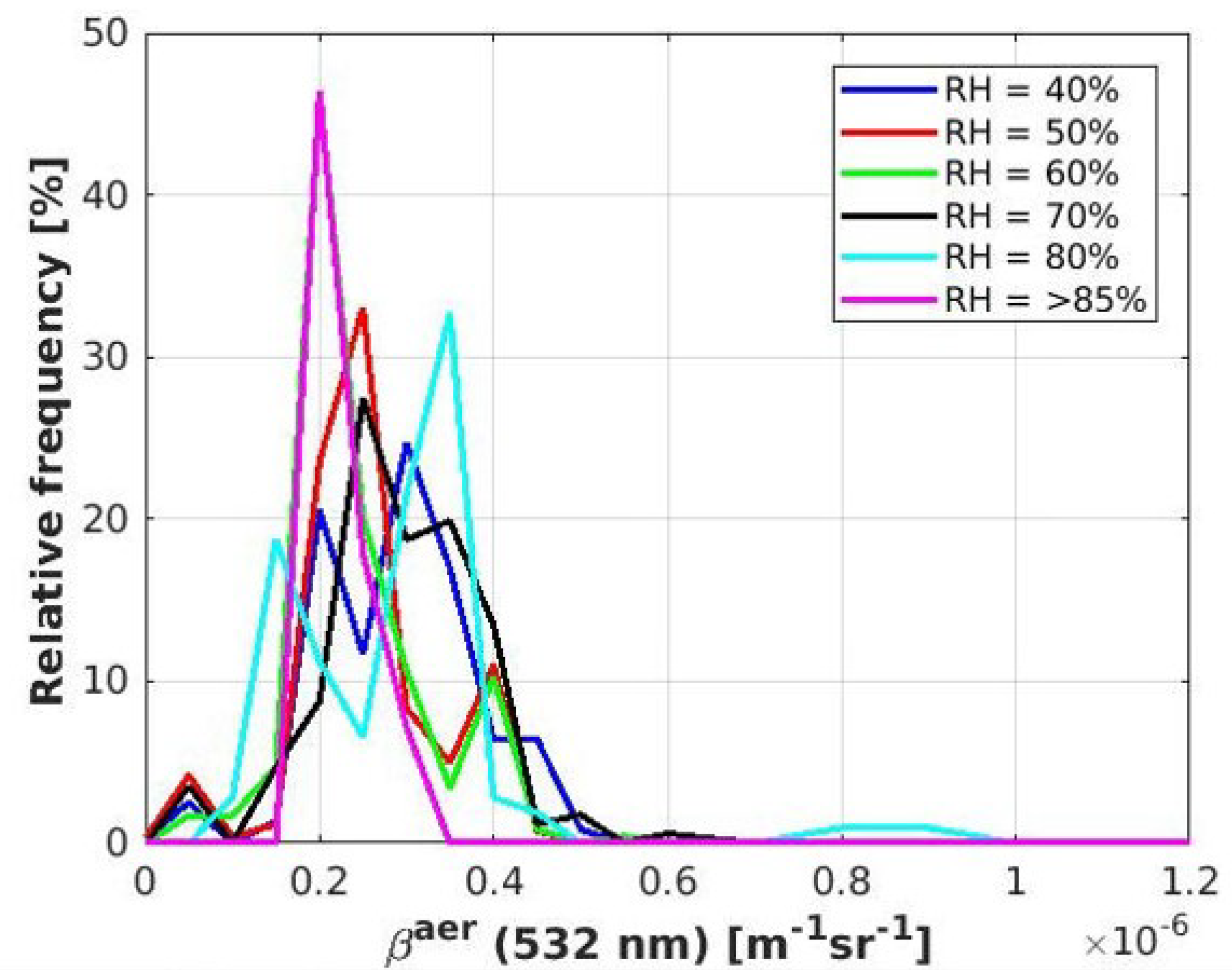
• A possible systematic bias between lidar and in situ measurements might be due to hygroscopic growth, which might partly be lost by warming and drying of the air flow in the inlets in Arctic conditions. However, no noticeable hygroscopic growth was found from synchronous lidar and radiosonde measurements. Higher than average backscatter values generally occurred at moderate relative humidity. Neither the aerosol backscatter coefficient nor the colour ratio showed any positive correlation to relative humidity. We conclude that obviously aerosol and moisture have different origins (pathways) and that part of the aerosol may have been washed out during its advection towards the remote site of Ny-Ålesund.
• Based on the lidar-derived uniform aerosol properties in the free troposphere and the high day-to-day variability of in situ-derived nss-sulphate concentration, we conclude that aerosol is mostly advected in the lowest free troposphere and mixed downward erratically into the shallow Arctic winter–spring boundary layer. Therefore, we hypothesize that the Arctic ground-based aerosol properties generally show higher temporal variability compared to the free troposphere. This implies that the comparison between lidar and ground-based in situ observations might be more reasonable on longer time scales, i.e., monthly and seasonal basis. The same holds true for the two in situ sites around Ny-Ålesund. Further studies on the boundary layer along the slope of Zeppelin mountain are needed to understand the reported differences in aerosol concentrations.

The complex orography may introduce implications in the comparison of point observations with regional climate models. It should be noted that the lidar site (Ny-Ålesund) and the two in situ stations (Gruvebadet and Zeppelin) are located only a few kilometers apart and, thus, within one grid cell of current regional climate models. Through comparing non-sea-salt sulphate concentration with lidar backscatter observations, we concluded that ground-based in situ and remote sensing data of the free troposphere around a site with complex orography generally does not agree. Therefore, the derivation of a sound observational aerosol product over Ny-Ålesund for input or validation of climate models remains an open task. Finally, the high climate sensitivity of the Arctic is of concern. Over the Zeppelin site, a shifting of aerosol from a polar towards a marine regime is already observed [52]. In combination with the intensified advection of warm and moist north Atlantic air masses [4] over Ny-Ålesund and the unusual warming by the west Spitsbergen current [53], the question whether current aerosol conditions will become typical in a warmer future Arctic becomes highly relevant.

Further, in the future, we aim at increased aerosol data coverage by extending our analysis to aerosol scenes with overlying cirrus clouds [54,55].

References

1. Serreze, M.; Francis, J. The Arctic Amplification Debate. Clim. Chang. 2006, 76, 241–264. [Google Scholar] [CrossRef] [Green Version]
2. Serreze, M.C.; Barry, R.G. Processes and impacts of Arctic amplification: A research synthesis. Glob. Planet. Chang. 2011, 77, 85–96. [Google Scholar] [CrossRef]
3. Cohen, J.; Screen, J.; Furtado, J.; Barlow, M.; Whittleston, D.; Coumou, D.; Francis, J.; Dethloff, K.; Entekhabi, D.; Overland, J.; et al. Recent Arctic amplification and extreme mid-latitude weather. Nat. Geosci. 2014, 7, 627–637. [Google Scholar] [CrossRef] [Green Version]
4. Dahlke, S.; Maturilli, M. Contribution of Atmospheric Advection to the Amplified Winter Warming in the Arctic North Atlantic Region. Adv. Meteorol. 2017, 2017, 1–8. [Google Scholar] [CrossRef] [Green Version]
5. Block, K.; Schneider, F.A.; Mülmenstädt, J.; Salzmann, M.; Quaas, J. Climate models disagree on the sign of total radiative feedback in the Arctic. Tellus A Dyn. Meteorol. Oceanogr. 2020, 72, 1–14. [Google Scholar] [CrossRef] [Green Version]
6. Wendisch, M.; Macke, A.; Ehrlich, A.; Lüpkes, C.; Mech, M.; Chechin, D.; Dethloff, K.; Barientos, C.; Bozem, H.; Brückner, M.; et al. The Arctic Cloud Puzzle: Using ACLOUD/PASCAL Multiplatform Observations to Unravel the Role of Clouds and Aerosol Particles in Arctic Amplification. Bull. Am. Meteorol. Soc. 2018, 100. [Google Scholar] [CrossRef]
7. Nakoudi, K.; Ritter, C.; Böckmann, C.; Kunkel, D.; Eppers, O.; Rozanov, V.; Mei, L.; Pefanis, V.; Jäkel, E.; Herber, A.; et al. Does the Intra-Arctic Modification of Long-Range Transported Aerosol Affect the Local Radiative Budget? (A Case Study). Remote Sens. 2020, 12, 2112. [Google Scholar] [CrossRef]
8. Kirsanov, A.; Rozinkina, I.; Rivin, G.; Zakharchenko, D.; Olchev, A. Effect of Natural Forest Fires on Regional Weather Conditions in Siberia. Atmosphere 2020, 11, 1133. [Google Scholar] [CrossRef]
9. Oshima, N.; Yukimoto, S.; Deushi, M.; Koshiro, T.; Kawai, H.; Tanaka, T.; Yoshida, K. Global and Arctic effective radiative forcing of anthropogenic gases and aerosols in MRI-ESM2.0. Prog. Earth Planet. Sci. 2020, 7. [Google Scholar] [CrossRef]
10. Sato, K.; Inoue, J.; Yamazaki, A.; Kim, J.H.; Maturilli, M.; Dethloff, K.; Hudson, S.R.; Granskog, M.A. Improved forecasts of winter weather extremes over midlatitudes with extra Arctic observations. J. Geophys. Res. Ocean. 2017, 122, 775–787. [Google Scholar] [CrossRef] [Green Version]
11. Stock, M.; Ritter, C.; Aaltonen, V.; Aas, W.; Handorff, D.; Herber, A.; Treffeisen, R.; Dethloff, K. Where does the optically detectable aerosol in the European Arctic come from? Tellus B 2014, 66. [Google Scholar] [CrossRef] [Green Version]
12. Quinn, P.K.; Shaw, G.; Andrews, E.; Dutton, E.G.; Ruoho-Airola, T.; Gong, S.L. Arctic haze: Current trends and knowledge gaps. Tellus B Chem. Phys. Meteorol. 2007, 59, 99–114. [Google Scholar] [CrossRef] [Green Version]
13. Di Pierro, M.; Jaeglé, L.; Eloranta, E.; Sharma, S. Spatial and seasonal distribution of Arctic aerosols observed by the CALIOP satellite instrument (2006–2012). Atmos. Chem. Phys. 2013, 13. [Google Scholar] [CrossRef] [Green Version]
14. Schmeisser, L.; Backman, J.; Ogren, J.; Andrews, E.; Asmi, E.; Starkweather, S.; Uttal, T.; Fiebig, M.; Sharma, S.; Eleftheriadis, K.; et al. Seasonality of aerosol optical properties in the Arctic. Atmos. Chem. Phys. Discuss. 2018, 1–41. [Google Scholar] [CrossRef] [Green Version]
15. Sharma, S.; Barrie, L.; Magnusson, E.; Brattström, G.; Leaitch, W.; Steffen, A.; Landsberger, S. A Factor and Trends Analysis of Multidecadal Lower Tropospheric Observations of Arctic Aerosol Composition, Black Carbon, Ozone, and Mercury at Alert, Canada. J. Geophys. Res. Atmos. 2019, 124, 14133–14161. [Google Scholar] [CrossRef] [Green Version]
16. Udisti, R.; Bazzano, A.; Becagli, S.; Bolzacchini, E.; Caiazzo, L.; Cappelletti, D.; Ferrero, L.; Frosini, D.; Giardi, F.; Grotti, M.; et al. Sulfate source apportionment in the Ny-Ålesund (Svalbard Islands) Arctic aerosol. Rend. Lincei 2016, 27. [Google Scholar] [CrossRef]
17. Lisok, J.; Markowicz, K.; Ritter, C.; Makuch, P.; Petelski, T.; Chilinski, M.; Kaminski, J.; Becagli, S.; Traversi, R.; Udisti, R.; et al. 2014 iAREA campaign on aerosol in Spitsbergen—Part 1: Study of physical and chemical properties. Atmos. Environ. 2016, 140, 150–166. [Google Scholar] [CrossRef] [Green Version]
18. Breider, T.J.; Mickley, L.J.; Jacob, D.J.; Ge, C.; Wang, J.; Payer Sulprizio, M.; Croft, B.; Ridley, D.A.; McConnell, J.R.; Sharma, S.; et al. Multidecadal trends in aerosol radiative forcing over the Arctic: Contribution of changes in anthropogenic aerosol to Arctic warming since 1980. J. Geophys. Res. Atmos. 2017, 122, 3573–3594. [Google Scholar] [CrossRef]
19. Hirdman, D.; Burkhart, J.F.; Sodemann, H.; Eckhardt, S.; Jefferson, A.; Quinn, P.K.; Sharma, S.; Ström, J.; Stohl, A. Long-term trends of black carbon and sulphate aerosol in the Arctic: Changes in atmospheric transport and source region emissions. Atmos. Chem. Phys. 2010, 10, 9351–9368. [Google Scholar] [CrossRef] [Green Version]
20. Collaud Coen, M.; Andrews, E.; Alastuey, A.; Arsov, T.P.; Backman, J.; Brem, B.T.; Bukowiecki, N.; Couret, C.; Eleftheriadis, K.; Flentje, H.; et al. Multidecadal trend analysis of in situ aerosol radiative properties around the world. Atmos. Chem. Phys. 2020, 20, 8867–8908. [Google Scholar] [CrossRef]
21. Grassl, S.; Ritter, C. Properties of Arctic Aerosol Based on Sun Photometer Long-Term Measurements in Ny-Ålesund. Remote Sens. 2019, 11, 1362. [Google Scholar] [CrossRef] [Green Version]
22. Ritter, C.; Angeles Burgos, M.; Böckmann, C.; Mateos, D.; Lisok, J.; Markowicz, K.; Moroni, B.; Cappelletti, D.; Udisti, R.; Maturilli, M.; et al. Microphysical properties and radiative impact of an intense biomass burning aerosol event measured over Ny-Ålesund, Spitsbergen in July 2015. Tellus B 2018, 70, 1–23. [Google Scholar] [CrossRef]
23. Shibata, T.; Shiraishi, K.; Shiobara, M.; Iwasaki, S.; Takano, T. Seasonal Variations in High Arctic Free Tropospheric Aerosols Over Ny-Ålesund, Svalbard, Observed by Ground-Based Lidar. J. Geophys. Res. Atmos. 2018, 123, 12353–12367. [Google Scholar] [CrossRef]
24. Zielinski, T.; Bolzacchini, E.; Cataldi, M.; Ferrero, L.; Graßl, S.; Hansen, G.; Mateos, D.; Mazzola, M.; Neuber, R.; Pakszys, P.; et al. Study of Chemical and Optical Properties of Biomass Burning Aerosols during Long-Range Transport Events toward the Arctic in Summer 2017. Atmosphere 2020, 11, 27. [Google Scholar] [CrossRef] [Green Version]
25. Tunved, P.; Ström, J.; Krejci, R. Arctic aerosol life cycle: Linking aerosol size distributions observed between 2000 and 2010 with air mass transport and precipitation at Zeppelin station, Ny-Ålesund, Svalbard. Atmos. Chem. Phys. 2013, 13, 3643–3660. [Google Scholar] [CrossRef] [Green Version]
26. Herber, A.; Thomason, L.W.; Gernandt, H.; Leiterer, U.; Nagel, D.; Schulz, K.H.; Kaptur, J.; Albrecht, T.; Notholt, J. Continuous day and night aerosol optical depth observations in the Arctic between 1991 and 1999. J. Geophys. Res. Atmos. 2002, 107, AAC-6. [Google Scholar] [CrossRef]
27. Ritter, C.; Neuber, R.; Schulz, A.; Markowicz, K.; Stachlewska, I.; Lisok, J.; Makuch, P.; Pakszys, P.; Markuszewski, P.; Rozwadowska, A.; et al. 2014 iAREA campaign on aerosol in Spitsbergen—Part 2: Optical properties from Raman-lidar and in-situ observations at Ny-Ålesund. Atmos. Environ. 2016, 141, 1–19. [Google Scholar] [CrossRef] [Green Version]
28. Tesche, M.; Zieger, P.; Rastak, N.; Charlson, R.; Glantz, P.; Tunved, P.; Hansson, H.C. Reconciling aerosol light extinction measurements from spaceborne lidar observations and in situ measurements in the Arctic. Atmos. Chem. Phys. 2014, 14. [Google Scholar] [CrossRef] [Green Version]
29. Ferrero, L.; Cappelletti, D.; Busetto, M.; Mazzola, M.; Lupi, A.; Lanconelli, C.; Becagli, S.; Traversi, R.; Caiazzo, L.; Giardi, F.; et al. Vertical profiles of aerosol and black carbon in the Arctic: A seasonal phenomenology along 2 years (2011–2012) of field campaigns. Atmos. Chem. Phys. 2016, 16, 12601–12629. [Google Scholar] [CrossRef] [Green Version]
30. Ferrero, L.; Ritter, C.; Cappelletti, D.; Moroni, B.; Močnik, G.; Mazzola, M.; Lupi, A.; Becagli, S.; Traversi, R.; Cataldi, M.; et al. Aerosol optical properties in the Arctic: The role of aerosol chemistry and dust composition in a closure experiment between Lidar and tethered balloon vertical profiles. Sci. Total Environ. 2019, 686, 452–467. [Google Scholar] [CrossRef] [Green Version]
31. Jocher, G.; Schulz, A.; Ritter, C.; Neuber, R.; Dethloff, K.; Foken, T. The Sensible Heat Flux in the Course of the Year at Ny-Ålesund, Svalbard: Characteristics of Eddy Covariance Data and Corresponding Model Results. Adv. Meteorol. 2015. [Google Scholar] [CrossRef]
32. Sicard, M.; Rodríguez-Gómez, A.; Comerón, A.; Muñoz-Porcar, C. Calculation of the Overlap Function and Associated Error of an Elastic Lidar or a Ceilometer: Cross-Comparison with a Cooperative Overlap-Corrected System. Sensors 2020, 20, 6312. [Google Scholar] [CrossRef]
33. Zieger, P.; Fierz-Schmidhauser, R.; Gysel, M.; Ström, J.; Henne, S.; Yttri, K.E.; Baltensperger, U.; Weingartner, E. Effects of relative humidity on aerosol light scattering in the Arctic. Atmos. Chem. Phys. 2010, 10, 3875–3890. [Google Scholar] [CrossRef] [Green Version]
34. Hoffmann, A. Comparative Aerosol Studies Based on Multi-Wavelength Raman LIDAR at Ny-Ålesund, Spitsbergen. Ph.D. Thesis, Alfred Wegener Institute, Potsdam, Germany, 2011. [Google Scholar]
35. Müller, K.J.; Ritter, C.; Nakoudi, K. Aerosol Investigation During the Arctic Haze Season of 2018: Optical and Hygroscopic Properties. In Proceedings of the EPJ Web Conference, Hefei, China, 24–28 June 2020; Volume 237, p. 02001. [Google Scholar]
36. Ansmann, A.; Wandinger, U.; Riebesell, M.; Weitkamp, C.; Michaelis, W. Independent measurement of extinction and backscatter profiles in cirrus clouds by using a combined Raman elastic-backscatter lidar. Appl. Opt. 1992, 31, 7113–7131. [Google Scholar] [CrossRef]
37. Behrendt, A.; Nakamura, T. Calculation of the calibration constant of polarization lidar and its dependency on atmospheric temperature. Opt. Express 2002, 10, 805–817. [Google Scholar] [CrossRef] [PubMed]
38. Giardi, F.; Traversi, R.; Becagli, S.; Severi, M.; Caiazzo, L.; Ancillotti, C.; Udisti, R. Determination of Rare Earth Elements in multi-year high-resolution Arctic aerosol record by double focusing Inductively Coupled Plasma Mass Spectrometry with desolvation nebulizer inlet system. Sci. Total Environ. 2018, 613–614, 1284–1294. [Google Scholar] [CrossRef]
39. Becagli, S.; Ghedini, C.; Peeters, S.; Rottiers, A.; Traversi, R.; Udisti, R.; Chiari, M.; Jalba, A.; Despiau, S.; Dayan, U.; et al. MBAS (Methylene Blue Active Substances) and LAS (Linear Alkylbenzene Sulphonates) in Mediterranean coastal aerosols: Sources and transport processes. Atmos. Environ. 2011, 45, 6788–6801. [Google Scholar] [CrossRef]
40. Groß, S.; Esselborn, M.; Weinzierl, B.; Wirth, M.; Fix, A.; Petzold, A. Aerosol classification by airborne high spectral resolution lidar observations. Atmos. Chem. Phys. 2013, 13, 2487. [Google Scholar] [CrossRef] [Green Version]
41. Benassai, S.; Becagli, S.; Gragnani, R.; Magand, O.; Proposito, M.; Fattori, I.; Traversi, R.; Udisti, R. Sea-spray deposition in Antarctic coastal and plateau areas from ITASE traverses. Ann. Glaciol. 2005, 41, 32–40. [Google Scholar] [CrossRef] [Green Version]
42. Udisti, R.; Traversi, R.; Becagli, S.; Tomasi, C.; Mazzola, M.; Lupi, A.; Quinn, P. Arctic Aerosols; Springer: Cham, Switzerland, 2020. [Google Scholar] [CrossRef]
43. Bowen, H.J.M. Environmental Chemistry of the Elements; Academic Press: Cambridge, MA, USA, 1979. [Google Scholar]
44. Becagli, S.; Lazzara, L.; Marchese, C.; Dayan, U.; Ascanius, S.; Cacciani, M.; Caiazzo, L.; Di Biagio, C.; Di Iorio, T.; di Sarra, A.; et al. Relationships linking primary production, sea ice melting, and biogenic aerosol in the Arctic. Atmos. Environ. 2016, 136, 1–15. [Google Scholar] [CrossRef] [Green Version]
45. Müller, K.J. Characterisation of Arctic Aerosols on the Basis of Lidar- and Radiometer-Data. Master’s Thesis, Alfred Wegener Institute, Potsdam, Germany, 2019. [Google Scholar]
46. Mazzola, M.; Tampieri, F.; Viola, A.; Lanconelli, C.; Choi, T. Stable boundary layer vertical scales in the Arctic: Observations and analyses at Ny-Ålesund, Svalbard. Q. J. R. Meteorol. Soc. 2016, 142, 1250–1258. [Google Scholar] [CrossRef]
47. Gryning, S.E.; Batchvarova, E. Marine Boundary Layer And Turbulent Fluxes Over The Baltic Sea: Measurements and Modelling. Bound. Layer Meteorol. 2002, 103, 29–47. [Google Scholar] [CrossRef]
48. Thomas, M.A.; Devasthale, A.; Tjernström, M.; Ekman, A.M.L. The Relation Between Aerosol Vertical Distribution and Temperature Inversions in the Arctic in Winter and Spring. Geophys. Res. Lett. 2019, 46, 2836–2845. [Google Scholar] [CrossRef] [Green Version]
49. Yamanouchi, T.; Treffeisen, R.; Herber, A.; Shiobara, M.; Yamagata, S.; Hara, K.; Sato, K.; Yabuki, M.; Tomikawa, Y.; Rinke, A.; et al. Arctic Study of Tropospheric Aerosol and Radiation (ASTAR) 2000: Arctic haze case study. Tellus B Chem. Phys. Meteorol. 2005, 57, 141–152. [Google Scholar] [CrossRef]
50. Stohl, A. Characteristics of atmospheric transport into the Arctic troposphere. J. Geophys. Res. Atmos. 2006, 111. [Google Scholar] [CrossRef]
51. Tomasi, C.; Kokhanovsky, A.A.; Lupi, A.; Ritter, C.; Smirnov, A.; O’Neill, N.T.; Stone, R.S.; Holben, B.N.; Nyeki, S.; Wehrli, C.; et al. Aerosol remote sensing in polar regions. Earth Sci. Rev. 2015, 140, 108–157. [Google Scholar] [CrossRef] [Green Version]
52. Heslin-Rees, D.; Burgos, M.; Hansson, H.C.; Krejci, R.; Ström, J.; Tunved, P.; Zieger, P. From a polar to a marine environment: Has the changing Arctic led to a shift in aerosol light scattering properties? Atmos. Chem. Phys. 2020, 20, 13671–13686. [Google Scholar] [CrossRef]
53. Walczowski, W.; Piechura, J. Influence of the West Spitsbergen Current on the local climate. Int. J. Climatol. 2011, 31, 1088–1093. [Google Scholar] [CrossRef]
54. Nakoudi, K.; Ritter, C. AWI Cirrus Cloud Retrieval Scheme (v1.0.0). 2020. Available online: https://zenodo.org/record/4265007#.YDMGnnkRWUk (accessed on 15 February 2021).
55. Nakoudi, K.; Stachlewska, I.S.; Ritter, C. An extended lidar-based cirrus cloud retrieval scheme: First application over an Arctic site. Opt. Express 2021, 20, 20. [Google Scholar] [CrossRef]
Figure 1. Site map of Ny-Ålesund. The locations of the Raman Lidar (1), the Gruvebadet Station (2) and the Zeppelin Station (3) are marked in the figure.
Atmosphere 12 00271 g001
Figure 2. 700–1500 m: Frequency of β 532 .
Atmosphere 12 00271 g002
Figure 3. 700–1500 m: Frequency of δ 532 .
Atmosphere 12 00271 g003
Figure 4. January–April: Frequency of β 532 .
Atmosphere 12 00271 g004
Figure 5. January–April: Frequency of the CR.
Atmosphere 12 00271 g005
Figure 6. January–April: Frequency of δ 532 .
Atmosphere 12 00271 g006
Figure 7. January–April: Frequency of the LR 355 .
Atmosphere 12 00271 g007
Figure 8. The colour ratio against the backscatter at 532 nm between 1500 and 2000 m altitude. The different colours indicate the corresponding RH ranges.
Atmosphere 12 00271 g008
Figure 9. The backscatter at 532 nm for different values of the RH between 1500 and 2000 m altitude. The different colours indicate the corresponding RH ranges.
Atmosphere 12 00271 g009
Figure 10. The colour ratio for different values of the RH between 1500 and 2000 m altitude. The different colours indicate the RH ranges.
Atmosphere 12 00271 g010
Figure 11. nssSO 4 2 concentrations for spring 2019 at the village (Gruvebadet) and the mountain (Zeppelin) station.
Atmosphere 12 00271 g011
Figure 12. SO 4 2 concentration from Gruvebadet station.
Atmosphere 12 00271 g012
Figure 13. SO 4 2 concentration from Zeppelin station.
Atmosphere 12 00271 g013
Figure 14. Source apportionment of SO 4 2 from Gruvebadet Station.
Atmosphere 12 00271 g014
Figure 15. Aerosol backscatter data from 1 to 13 of March 2018 (Müller [45]) in comparison to the data from this study (all available data from March 2019). The filled lines (in italic) represent the 2018 data, while the dashed lines represent the 2019 data (this study).
Atmosphere 12 00271 g015
Figure 16. Comparing the colour ratios from 1 to 13 of March 2018 (Müller [45]) in comparison to the data from this study (all available data from March 2019). The filled lines (in italic) represent the 2018 data, while the dashed lines represent the 2019 data (this study).
Atmosphere 12 00271 g016
Figure 17. Comparing the depolarisation ratios from 1 to 13 of March 2018 (Müller [45]) in comparison to the data from this study (all available data from March 2019). The filled lines (in italic) represent the 2018 data, while the dashed lines represent the 2019 data (this study).
Atmosphere 12 00271 g017
Figure 18. Boundary layer altitude from local radiosonde using the bulk Richardson number.
Atmosphere 12 00271 g018
Figure 19. Correlation between nss-SO 4 2 concentration at both in situ sites.
Atmosphere 12 00271 g019
Figure 20. Relation between nss-SO 4 2 concentration and PM10 from Gruvebadet station for low PM10 load.
Atmosphere 12 00271 g020
Figure 21. Relation between nss-SO 4 2 concentration and PM10 from Gruvebadet station for high PM10 load.
Atmosphere 12 00271 g021
Figure 22. Averaged aerosol backscatter in three different altitude intervals.
Atmosphere 12 00271 g022
Publisher’s Note: MDPI stays neutral with regard to jurisdictional claims in published maps and institutional affiliations.