Article

A Multi-Fidelity Framework for Wildland Fire Behavior Simulations over Complex Terrain

1
National Institute of Standards and Technology, Gaithersburg, MD 20899, USA
2
U.S. Forest Service, Seattle, WA 98103, USA
3
Corpo Nazionale dei Vigili del Fuoco, 17100 Savona, Italy
4
CIMA Research Foundation, 17100 Savona, Italy
*
Authors to whom correspondence should be addressed.
Atmosphere 2021, 12(2), 273; https://doi.org/10.3390/atmos12020273
Submission received: 7 January 2021 / Revised: 25 January 2021 / Accepted: 2 February 2021 / Published: 18 February 2021
(This article belongs to the Special Issue Coupled Fire-Atmosphere Simulation)

Abstract

:
A method for the large-eddy simulation (LES) of wildfire spread over complex terrain is presented. In this scheme, a cut-cell immersed boundary method (CC-IBM) is used to render the complex terrain, defined by a tessellation, on a rectilinear Cartesian grid. Discretization of scalar transport equations for chemical species is done via a finite volume scheme on cut-cells defined by the intersection of the terrain geometry and the Cartesian cells. Momentum transport and heat transfer close to the immersed terrain are handled using dynamic wall models and a direct forcing immersed boundary method. A new “open” convective inflow/outflow method for specifying atmospheric wind boundary conditions is presented. Additionally, three basic approaches have been explored to model fire spread: (1) Representing the vegetation as a collection of Lagrangian particles, (2) representing the vegetation as a semi-porous boundary, and (3) representing the fire spread using a level set method, in which the fire spreads as a function of terrain slope, vegetation type, and wind speed. Several test and validation cases are reported to demonstrate the capabilities of this novel wildfire simulation methodology.

1. Introduction

In the past few decades, wildland and wildland-urban interface (WUI) fires have received substantial attention due to their destructive nature and extensive cost to lives and property [1,2,3]. A large body of literature can be found on the subject, as seen in various review articles [2,4,5]. Due to the complex nature of fire, limited computing resources, and the needs of planners and first responders, most models of wildfires have historically relied on simplified field-tested rules and correlations. Among these, the rate of the spread model of Rothermel [6] assumes quasi-steady-state surface fire conditions, and takes, as input, fuel properties, wind, terrain slope, and moisture that can be measured in situ. Fuel models have been cataloged [7], and their parameters defined so that model users can select and combine the most appropriate listed fuels. Rothermel’s rate of spread formula is still widely used, and has been implemented in several simulation tools [8,9,10,11,12,13,14,15,16,17,18], enabling a range of planning and operational forecasting capabilities.
Wildland fire modeling typically focuses on tracking the fire front, which can have a complex shape that moves and deforms based on local conditions, like fuel loading, moisture content, wind, and terrain. The fire front requires a mathematical representation. The Lagrangian approach is based on a polygonal mesh of control markers that represents the front [8,9]. On the other hand, an Eulerian representation allows for a fixed two-dimensional mesh on which the fire front is defined implicitly by a scalar field. This scalar field is called the level set function, and numerical methods that compute the function are called level set methods (LSM) [19,20]. Some wildfire solvers that use LSM to track the fire front are described in the References [9,10,13,14]. A practical comparison of the two techniques, as implemented in the Fire Dynamics Simulator (FDS) [21] and FARSITE [8], is provided in Ref. [9].
Because the spread rate of the fire front depends in part on the local wind conditions, a well-resolved wind field over complex terrain should improve the accuracy of the overall model. The de facto physics-based technique for practical simulation of wind is the Large Eddy Simulation (LES) [14,21,22]. For fire simulation over complex terrain, a range of techniques are being developed, in particular, in the coupling of the fire and the wind. For fast simulation of outdoor fires, an immersed boundary method has been interfaced with a level set scheme [9] and the Rothermel fire spread model. The wind speed input for Rothermel’s model results from the local velocity over the terrain which is affected by fire buoyancy and flow evolution. These are, in turn, also influenced by wind atmospheric conditions, accounted for within simulations using a mean wind forcing concept. This is a first step at implementing a level set approach in an LES wind calculation with combustion. It is recognized that in the empirically based development of the Rothermel formula, the wind speed is not influenced by the local buoyancy-induced flow.
A number of other approaches to modeling fire spread over complex terrain exist. A recent review, with an emphasis on operational applications, is given in [23]. A range of approximations to modeling both wind and fire have been employed. The uniqueness of the approach presented here is that, within a single computational tool, a range of approximations to the wind and fire physics can be employed. This can support a direct comparison between models of varying physical fidelity. For example, one can investigate the difference in predicted fire behavior between a simulation that models fire spread and heat release via the explicit accounting of the thermal degradation of vegetation and one that approximates fire spread via an empirically based model.
In the following section, the mathematical model for fire spread over complex terrain is described. The description of the terrain discretization is provided in Section 3. The various fire spread methods are described in Section 4, and the atmospheric boundary conditions in Section 5. Some flat terrain simulations are compared to experimental data, and a complex terrain simulation is compared to an actual wildfire in Section 6.

2. Mathematical Model

2.1. Governing Equations

For fire modeling in the gas phase, FDS employs a low Mach approximation for thermally driven buoyant and stratified flows [24]. Under this assumption, the pressure field p can be viewed as the summation of two components: a background hydrostatic pressure field p ¯ ( z , t ) used in the equation of state (ideal gas law), and a hydrodynamic pressure p ˜ ( x , y , z , t ) driving fluid motion.
Consider a mixture composed of N chemical species α , moving on a fixed point x in space with a mass weighted average velocity u ( x , t ) . If ρ ( x , t ) is the mixture density, the mass fraction for species α is Y α = ρ α / ρ , where ρ α ( x , t ) is the species mass density and ρ = ρ α . The scalar transport and momentum equations take the form:
ρ Y α t + · ( ρ Y α u ) = · J d α + m ˙ α + m ˙ b , α , α = 1 , , N
u t u × ω + H p ˜ 1 / ρ = 1 ρ ( ρ ρ 0 ) g + f b + · τ d e v ,
where J d α = ρ D α Y α is the diffusive flux for component α . Fick’s Law for binary diffusion with respect to a background species is assumed, and D α is the diffusivity of α with respect to the background species. Mass fractions Y α , solution of Equation (1), must obey realizability constraints 0 < Y α < 1 and α Y α = 1 . In Equation (1) starting from a realizable solution, realizability implies α J d α = 0 . Therefore, to enforce realizability, errors in diffusive transport are lumped into the most abundant species locally [25]. The volumetric combustion source term for species α is m ˙ α ( x , t ) ; the term m ˙ b , α is the contribution to species α from subgrid particle gasification. These correspond to the amount of mass per unit volume and time of species α being added or subtracted in a given point x due to chemical reaction or gasification of solid particles (or droplets), respectively. Details of the combustion model are provided below in Section 2.2.
In the momentum equation, the term H = | u | 2 / 2 + p ˜ / ρ , p ˜ is the perturbation pressure, and ρ 0 ( z ) is the modeled height-dependent background density of the atmosphere. Additionally, ω refers to the vorticity field. The gravity vector is g = ( 0 , 0 , g z ) , the buoyancy force term is ( ρ ρ 0 ) g , f b is the term contributed by modeled particle drag forces, and τ d e v is the deviatoric stress tensor accounting for molecular and subgrid turbulent stresses parameterized by an effective eddy viscosity model, discussed below in Section 2.2.
Conservation of energy is achieved by forcing the flow field to obey the following thermodynamic divergence constraint:
( · u ) th = 1 ρ c p T 1 p ¯ p ¯ t + w ρ 0 g z ρ c p T   + 1 ρ c p T q ˙ + q ˙ b · q ˙ · q ˙ r u · ( ρ h s )   + 1 ρ α W ¯ W α h s , α c p T m ˙ α + m ˙ b , α · ( J d α ) u · ( ρ Y α ) ,
where h s , α is the sensible enthalpy of species α , and h s is the sensible enthalpy of the mixture, q ˙ , q ˙ b are heat release rates due to combustion and particle gasification, T is the local gas temperature, and w is the local vertical velocity. The mixture-specific heat at constant pressure and molecular weight are c p = α = 1 N c p , α Y α and W ¯ = α = 1 N Y α / W α 1 , respectively. This thermodynamic divergence is derived from and acts as a proxy for the sensible enthalpy evolution equation [26]. Equation (3) is derived by factoring the divergence from the sensible enthalpy equation and applying the ideal gas law. Given a background pressure and a local mass density, the local temperature is computed from the ideal gas law as T = p ¯ W ¯ / ( ρ R ) .
The term q ˙ in Equation (3) represents the conductive and diffusive heat fluxes discussed in Section 2.2. The net contribution from thermal radiation in the energy equation is defined by:
· q ˙ r ( x ) = κ ( x ) U ( x ) 4 π I b ( x ) ; U ( x ) = 4 π I ( x , s ) d s ,
where κ ( x ) is the absorption coefficient, I b ( x ) is the source term, and I ( x , s ) is the solution of the radiation transport equation (RTE) for a non-scattering gray gas:
s · I ( x , s ) = κ ( x ) I b ( x ) I ( x , s ) .
The source term, I b , requires special treatment because of the limited resolution of the underlying numerical grid in the vicinity of flames. In large-scale fire simulations, grid cells are typically on the order of tens of centimeters. Flame sheets cannot be resolved, meaning that the computed cell-average temperature can be significantly lower than temperatures one would expect to find in the reacting flame. Consequently, the source term is approximated in grid cells where fuel and oxygen react. Elsewhere, the subgrid temperature field is homogeneous, and the source term can be computed directly:
κ I b = κ σ T 4 / π Outside flame zone , q ˙ = 0 C κ σ T 4 / π Inside flame zone , q ˙ > 0 .
The constant C is computed at each time step so that the volume integral of Equation (4) over the entire flaming region is approximately equal to the volume integral of χ r q ˙ over that same region. Here, χ r is an empirical estimate of the global fraction of that energy emitted as thermal radiation. Typically, a sooty fire radiates approximately one-third of the total combustion energy.
The radiation equation is solved using a technique similar to a finite volume method for convective transport, thus the name given to it is the Finite Volume Method (FVM). Using approximately 100 discrete angles which are updated over multiple time-steps, the finite volume solver requires about 20% of the total CPU time of a calculation, a modest cost given the complexity of radiation heat transfer.
Section 4.1 discusses how Lagrangian particles are used to represent vegetation like leaves, pine needles, and other subgrid objects. These particles absorb and emit thermal radiation, and the underlying assumptions are described in that section.

2.2. Subgrid Parameterizations

In the formal derivation of the LES equations (see, e.g., [27,28]) the filtered nonlinear terms (advection terms, mean chemical source term, and the unresolved boundary fluxes) require subgrid-scale parameterizations. In this section, LES filter notation, as well as Cartesian tensor index notation, are used to clarify the terms used in the governing equations.

2.2.1. Subgrid Advection

Unresolved turbulent eddies enhance the transport of mass, momentum, and energy. This added transport is accounted for with residual stresses and scalar fluxes. The subgrid-scale stress tensor is defined as
τ i j s g s ρ ¯ ( u i u j ˜ u ˜ i u ˜ j ) ,
where an overline represents a volumetric filter and the tilde represents a Favre filter (see, e.g., [29]).
In FDS, the deviatoric part of the subgrid stress tensor is modeled using the gradient diffusion hypothesis. Thus, the combined deviatoric stress may be written as follows:
τ i j d e v = τ ¯ i j + τ i j s g s 1 3 τ k k s g s = 2 ( μ + μ t ) S ˜ i j 1 3 S ˜ k k ,
where the symmetric rate-of-strain tensor is S i j 1 2 ( u i / x j + u j / x i ) , and μ t is an isotropic eddy viscosity. Note that τ ¯ i j is already the deviatoric part of the molecular stress as the isotropic part is the pressure; μ is the molecular dynamic viscosity.
The eddy viscosity μ t is an important quantity in the simulation, as it affects all the turbulent transport and subgrid mixing time-scales, which, as shown below, are crucial to the combustion model. In FDS, the eddy viscosity is modeled as [27,30]
μ t = ρ ¯ C ν Δ k s g s ,
with the constant taken as C ν = 0.1 (this value can be derived, assuming production equals dissipation and a model Kolmogorov spectrum [27]; the model is also tested against decaying isotropic turbulence [31]). In practice, the filter scale Δ is taken as the cube root of the cell volume. Deardorff [30] solved a transport equation for the subgrid kinetic energy per unit mass, k s g s , in order to account for subgrid buoyancy. In FDS, the density field is sufficiently resolved to account for buoyant plume accelerations, and therefore it is found that an algebraic closure for k s g s is sufficient. Following the work of Bardina [32], a scale-similarity idea is used; the subgrid kinetic energy per unit mass is modeled as follows:
k s g s = 1 2 ( u ˜ i u ˜ ^ i ) ( u ˜ i u ˜ ^ i ) ,
where the hat represents a test filter at a scale 2 Δ . For the first Cartesian cell off the wall, where a test filter is not well-defined, the eddy viscosity is taken from the WALE model [33].
Subgrid advection of mass and heat are also modeled using gradient diffusion. The turbulent diffusivities use constant turbulent Schmidt and Prandtl numbers, both set to 0.5; this simplification is justified based on high-resolution simulations of fire plumes (see, e.g., [34]). For mass diffusion of species α in direction i, the flux is
J α , i = J ¯ α , i + J α , i s g s = ρ ¯ ( D α + μ t Sc t ) Y ˜ α x i .
Effective thermal conductivity and mass diffusivity are used in the heat flux, which may be written as
q ˙ i = ( k ¯ + μ t c ¯ p Pr t ) T ˜ x i α h ˜ s , α ( ρ ¯ D α + μ t Sc t ) Y ˜ α x i .

2.2.2. Filtered Chemical Source Term

FDS treats combustion chemistry using a simplified approach. Only fuel, air, and products, referred to as “lumped species”, are tracked. Lumped species are groups of species that transport and react together and are always found in the same proportion. For example, air is a lumped species made up of 23% O 2 and 77% N 2 by mass. For vegetation, a surrogate hydrocarbon, fuel, is usually assumed. For example, cellulose may be assumed to decompose to a volatile fuel gas with the formula C6H10O5. The products are defined stoichiometrically, often including prescribed yields of soot (for smoke) and carbon monoxide that may be obtained from empirical relationships for the specific fuel or from other sources (e.g., [35]). Then, usually, a single reaction is tracked (more complicated reaction schemes are possible in the code, but for this work, a single reaction is sufficient):
Fuel + s Air ( 1 + s ) Products ,
where s is the mass stoichiometric coefficient.
In LES of turbulent combustion, the filtered chemical source term, m ˙ α ¯ , is unclosed because the reaction kinetics are nonlinear functions of species concentration and temperature. However, since the heat-releasing reactions in a fire are extremely fast compared to the time scales for turbulent mixing, it is common practice in fire dynamics simulations to utilize the eddy dissipation model of Magnussen and Hjertager [36] (see also [29]). The mass production term for the fuel species is written as
m ˙ F ¯ = ρ ¯ min ( Y ˜ F , Y ˜ A / s ) τ m i x .
This formula states that the fuel is consumed at a rate proportional to the local limiting reactant concentration, and inversely proportional to the local mixing time-scale. This is the so-called “mixed is burnt” approximation. The mixing time-scale is given by τ m i x = min ( τ d , τ u , τ g ) [37], where the time-scales for diffusion, turbulent advection, and gravitational acceleration are, respectively,
τ d = Δ 2 / D F
τ u = C u Δ / ( 2 / 3 ) k s g s
τ g = 2 Δ / g .
Here, D F is the binary diffusivity of the fuel species in air, k s g s is the modeled subgrid kinetic energy per unit mass discussed above, and g is the gravitational acceleration. The constant C u = 0.4 is determined by matching flame height correlations across a wide range of fire Froude numbers [28].
The remaining mass production rates are found from stoichiometry. The local heat release rate, q ˙ , an important term in Equation (3), is then determined from
q ˙ = α m ˙ α ¯ Δ h f , α ,
where Δ h f , α are the heats of formation for each lumped species α .

Flame Extinction

One of the advantages of a physics-based tool like FDS is the possibility of building into the model the effects of defensive actions on the fire spread rate. FDS uses simple empirical rules to predict local extinction within a gas phase grid cell based on resolved species concentrations and the mean cell temperature. The rules are based on the concept of a critical flame temperature. The basic theory behind the critical flame temperature is described in [38]. In brief, if the local heat release given by Equation (18) is not sufficient to raise the cell temperature above the CFT, then m ˙ F ¯ is set to zero for that cell for that time-step. Note that the flame extinction model does not directly affect surface cooling or smothering of the vegetative fuel, which may happen with certain fire suppression activities. However, such tactics can be accounted for through modifications to the solid fuel thermal degradation model discussed below.

2.2.3. Unresolved Boundary Fluxes

In this section, the wall functions used to close the mass, momentum, and energy fluxes on solid boundaries are discussed. Mass transfer of moisture and fuel from the surface is discussed in more detail below in Section 4, where the various flames spread models are compared (which is really the main focus of this paper).
The scaled streamwise velocity is denoted u + = u / u τ , where the friction velocity is u τ τ w / ρ and τ w is the wall stress needed to close the momentum equation, Equation (2). For rough walls, FDS employs the log law presented in [27],
u + = 1 κ ln y s + B ˜ ( s + ) ,
where κ = 0.41 is the von Kármán constant, s + = s / δ ν is the roughness length in viscous units, s is the dimensional “sand grain” roughness, and δ ν = μ / ( ρ u τ ) is the viscous length scale. The distance to the wall, y, is taken as δ y / 2 for the first off-wall grid cell. The parameter B ˜ varies with s + but attains a constant value B 2 = 8.5 in the fully rough limit. In FDS, B ˜ is implemented as the following piece-wise function:
B ˜ = B + ( 1 / κ ) ln ( s + ) for s + < 5.83 B ˜ max for 5.83 s + < 30.0 B 2 for s + 30.0 ,
where B ˜ max = 9.5 .
In the fully rough limit, the sand grain roughness may be equated to the aerodynamic roughness, z 0 , typically employed in atmospheric codes for a neutral boundary layer,
s = z 0 e 8.5 κ 32.6 z 0 .
It is important to appreciate that FDS was originally designed to handle compartment fires and must consider flows with smooth walls, such as HVAC ducts. Further, FDS typically resolves the thermal motions that would necessitate the use of Monin–Obukhov stability corrections to the boundary profile.
The unresolved heat flux at the surface, q ˙ w , is determined using an engineering approach,
q ˙ w = h ( T g T w ) ,
where h is the convective heat transfer coefficient, T w is the local temperature of the surface, and T g is the temperature of the first gas phase cell off the wall. Empirical natural/forced convection correlations are used to determine h:
h = max C | T g T w | 1 / 3 , k L Nu , k δ n / 2 ,
where C is a empirical coefficient for natural convection (1.52 for a horizontal plate and 1.31 for a vertical plane or cylinder) [39], L is a characteristic length related to the size of the physical obstruction, and k is the thermal conductivity of the gas. The forced convection Nusselt number (Nu) depends on the geometry and flow characteristics [39,40]. Further details are provided in [28].
Again, this simple approach is viable because FDS usually resolves the thermal flow fields that would necessitate added complexity. However, future work is planned to explore improvements to wall functions that may lead to better results at coarser grid resolution.

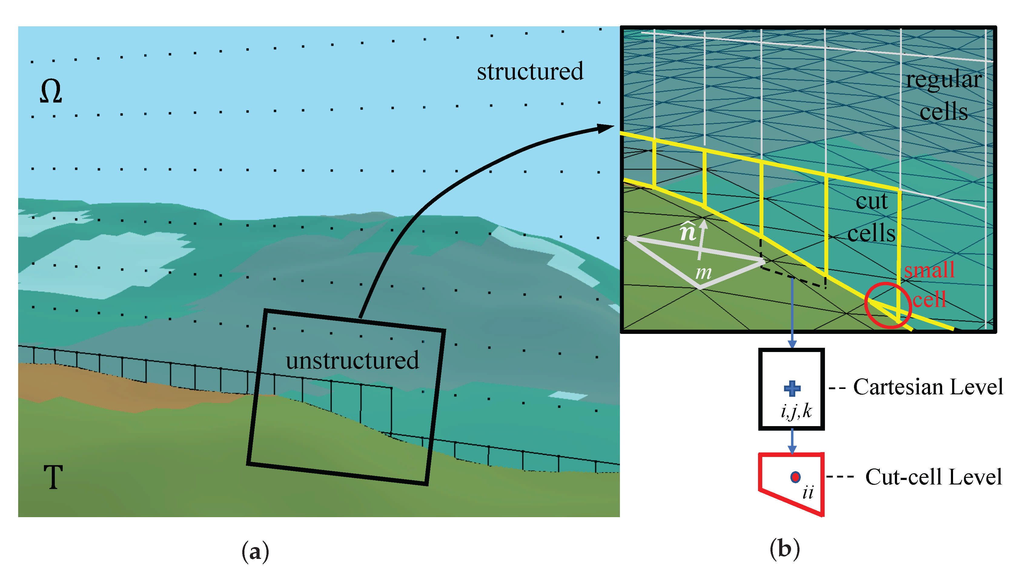
3. Terrain Description and Discretization

In Figure 1, the terrain is represented by its surface triangulation within an FDS Cartesian mesh. Some Cartesian cells and faces belonging to this mesh are transversed by the terrain surface. The remaining polyhedra and polygons that lie on the gas side of these intersected geometries are called cut-cells and cut-faces. They discretize the fluid domain in the region surrounding the solid surface. A detail of this unstructured mesh is shown in Figure 1. The resulting cut-cells and cut-faces are of various sizes and shapes, and situations where there are more than one cut-cell per Cartesian cell are common. As described later, small cells impose a temporal stability constraint on explicit time integration schemes. A two-level grid refinement hierarchy emerges. The coarse level is defined by the Cartesian entities, whereas the fine level is defined by the cut-cell or unstructured components. Methods that solve discrete model equations on these grids are called cut-cell or embedded boundary methods [41]. Reliably defining the cut-cell mesh geometric properties and topology is a complex problem in and of itself, but beyond the scope of this paper.

3.1. Cut-Cell Scalar Transport and Energy Discretization

The equations for chemical species transport are discretized using the finite volume method (FV) [42,43], as outlined in the diagram of Figure 2. Integrating Equation (1) over a cut-cell i i with control volume Ω i i gives:
Ω i i ρ Y α t d V + Ω i i · ρ Y α u d V = Ω i i · J d α d V + Ω i i m ˙ α + m ˙ b , α d V .
For a cut-cell control volume, the time derivative and source terms are approximated by
Ω i i ρ Y α t d V ρ Y α ¯ i i t V i i ; Ω i i m ˙ α + m ˙ b , α d V m ˙ α ¯ i i + m ˙ b , α ¯ i i V i i ,
where V i i is the volume of cell i i and the overlines imply cell averages. In the following, the notation is simplified by dropping overlines, observing that quantities are cell- or face-averaged. Consider the FV discretization of the diffusive term of Equation (24) on cut-cell i i of Figure 2:
Ω i i · J d α d V = Ω i i ρ D α Y α · n ^ i i d S = k = 1 n f ρ D α Y α k · n ^ i i , k A k .
The integral over the cut-cell volume has been transformed in an area integral on its n f = 5 faces using the divergence theorem. As these k-faces with areas A k and outward normals n ^ i i , k are planar by construction, the method for evaluation of their mean diffusive fluxes ρ D α Y α k will define the spatial accuracy of the discretization. Centroid to centroid (i.e., Δ x cc in Figure 2) finite differences and linear interpolation are used to approximate Y α and ρ D α for each face belonging to the gas phase. Additionally, a normal probe approach [44], is employed to sample information from the fluid to define fluxes in boundary cut-faces. In a normal probe method, an external point is defined at a normal distance from the body of the order of the cartesian grid size. Then, information from the fluid at this external point is obtained via interpolation.
Similarly, the discretization of the advective term is:
Ω i i · ρ Y α u d V = Ω i i ρ Y α u · n ^ i i d S k = 1 n f ρ Y α u k · n ^ i i , k A k ,
where the advective flux for face k is ρ Y α u k = [ ρ Y α ] ¯ k u k , and the over bar in [ ρ Y α ] ¯ k means it is a flux-limited interpolation to the cut-face [10]. In the cut-cell region, a Godunov flux limited interpolation for the advective term is used. Flux-limited interpolation is one of the fundamental components of stable numerical schemes for hyperbolic equations [43], of which mass transport inherits its mathematical properties. The time integration scheme in FDS is an explicit Runge-Kutta (RK2) method, all variables in the right-hand side of Equations (26) and (27) are assumed to be known. Explicit Runge–Kutta time integration methods are single-step multistage schemes widely used for advancing ordinary and partial differential equations [45]. The FV counterpart of the thermodynamic divergence expression for cut-cell i i is:
( · u ) i i th V i i = 1 ( ρ c p T ) i i 1 p ¯ i i p ¯ i i t V i i + w i i ρ 0 g z ( ρ c p T ) i i V i i   + 1 ( ρ c p T ) i i ( q ˙ + q ˙ b ) i i V i i k = 1 n f q ˙ i i , k · n ^ i i , k A k u · ( ρ h s ) ¯ V i i   + 1 ρ i i α W ¯ W α h s , α c p T i i ( m ˙ α + m ˙ b , α ) i i V i i k = 1 n f J α , i i , k · n ^ i i , k A k u · ( ρ Y α ) ¯ V i i ,
where the over-line terms refer to flux-limited interpolation of corresponding scalars, and terms defined with subscript i i refer to cell-defined quantities. All heat and mass fluxes and scalars are assumed to be known. Additionally, the vertical velocity w i i is interpolated to the cut-cell centroid. Details of the FDS time-integration scheme can be found in the References [10,26]. For each RK2 substep, the species transport equations are advanced in all FDS Cartesian cells, and then the solution (explicit fluxes and scalar densities) is recomputed on the unstructured cut-cell region. A similar procedure is done for the thermodynamic divergence. As an explicit time-integrator is used, in general, there will arise cut-cells whose small size will severely penalize the time-step. These cut-cells are linked to larger surrounding cells. Cell-linking, in the context of momentum equations, can be found in the Reference [46]. In FDS, the momentum equations and pressure Poisson equation are solved on the Cartesian mesh. Therefore, an immersed boundary method is used to reconstruct velocities in the cut-cell region. A divergence integral equivalence argument is used to transfer the divergence from cut-cells to the underlying Cartesian cells in order to build the source term of the Poisson equation for the pressure.

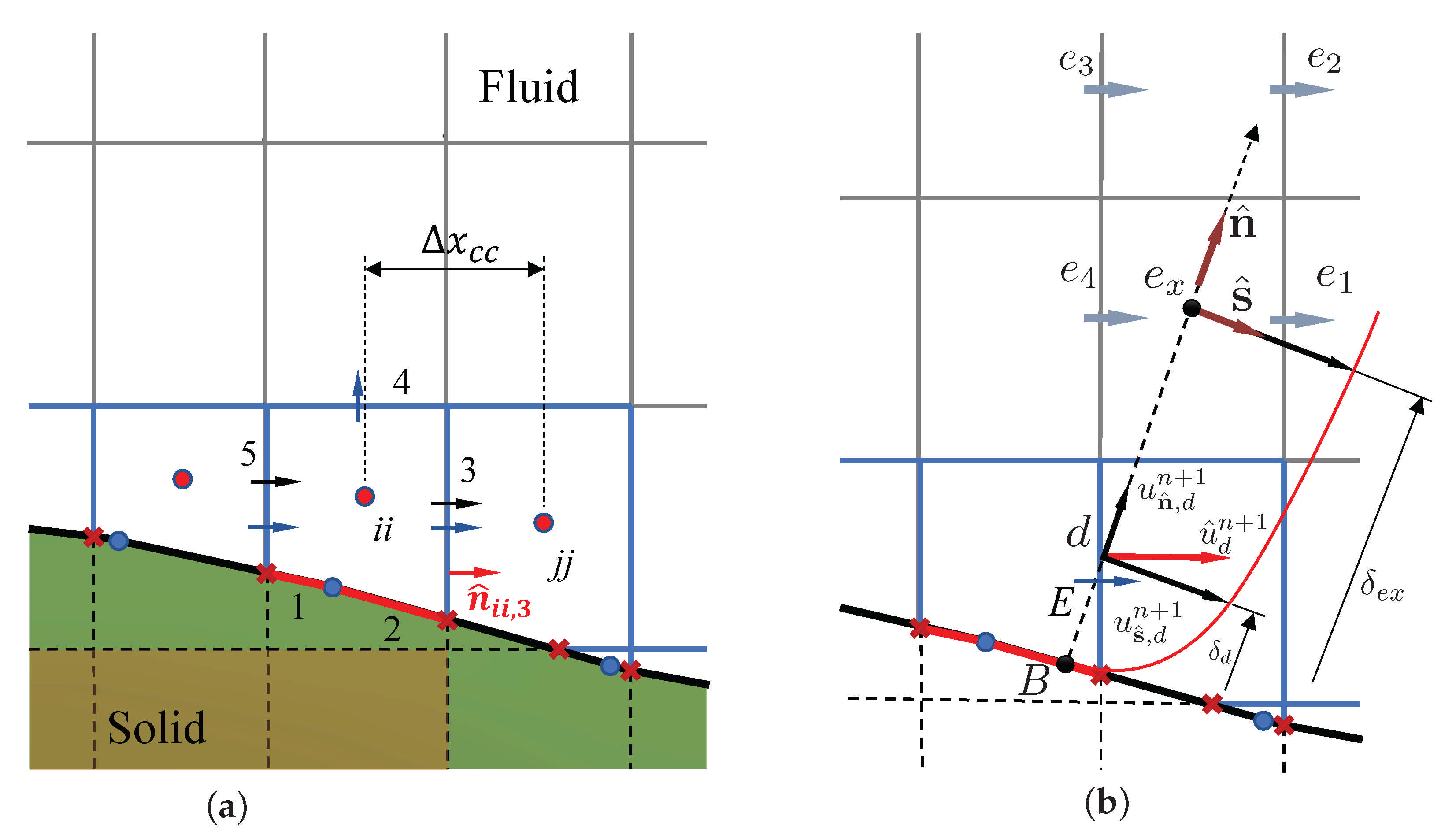
3.2. Immersed Boundary Method and Wall Modeling

Collecting advective, shear stress, and force terms in F ( u , x , t ) within Equation (), the model momentum transport problem can be written as [10]:
u ( x , t ) t = F ( u , x , t ) H ( x , t )
· u ( x , t ) = · u th ,
where Equation (29) is the momentum equation, subject to a specified divergence field, provided by Equation (3). Boundary conditions are prescribed for u ( x , t ) on boundaries, including the immersed terrain.
The previous equations are advanced in time using a fractional step method. As an illustration, consider their Forward Euler (FE) update from t n to t n + 1 = t n + Δ t . Given u n = u ( x , t n ) , · u th , n + 1 are known:
u n + 1 u n Δ t = F n H n
· u n + 1 = · u th , n + 1 ,
where u n + 1 represents a numerical solution at time t n + 1 . This discrete FE update corresponds to the first sub-step of the FDS explicit RK2 integrator. The potential field H ( x , t ) does not have a time evolution equation, and it is responsible for enforcing the divergence condition and is used on the projection step. Taking the divergence of Equation (31) and considering the constraint, Equation (32), the two steps of the method are:
  • Solve Poisson equation for H n :
    · H n = · u th , n + 1 · u n Δ t · F n .
  • Obtain final velocity for step:
    u n + 1 = u n Δ t F n + H n .
A consequence of the projection scheme is that boundary conditions are required on the Poisson equation, Equation (33). For explicit methods and stationary solid boundaries, the corresponding boundary condition is homogeneous Neumann for H n in Ω , Ω 1 , . . . , Ω nbods [47]. Next, an approximation to the no-slip boundary condition at the immersed terrain surface is needed. To this end, a direct forcing immersed boundary method (IBM) for the momentum equations [48] is employed. A force field is computed on the discrete momentum equations on grid faces crossed by the immersed surfaces to approximate the no-slip boundary condition on these. In LES, the surrounding velocity field is modeled using an equilibrium boundary layer solution.
In Figure 2, the velocity update in each of the gas phase cut-face centroids d is done by individualizing point B on the boundary and the normal direction through these. Additionally, an external point e x through the normal n ^ is defined at a distance δ e x , of the order of the Cartesian cells’ size. Known velocities and fluid parameters are interpolated from the surrounding fluid points e 1 , , e 4 to e x . This information is used to estimate a target velocity at step n + 1 , u ^ d n + 1 , k 1 at point d, assuming the log law equilibrium boundary layer solution of Section 2.2.3. The target velocity u ^ d n + 1 , k 1 component on the cut-face centroid is flux-matched to the underlying Cartesian face E velocity component u ^ E n + 1 , k 1 . Finally, an immersed boundary force
F E k = u ^ E n + 1 , k 1 u E n Δ t H n , k 1 x
can be computed and used in Equation (33) to take into account the presence of the body. The index k refers, in this context, to the sub-iteration that can be performed in the IB force, Equation (35), and projection, Equations (33) and (34), to match final velocities with the wall-modeled targets. This velocity reconstruction procedure has been combined with the level set method for fire spread described in the next section.

4. Wildland Fire Spread

There are various types of wildland fire spread models to choose from, and the choice depends on the desired level of physical fidelity and the available computing resources. The choice also depends on the nature of the fire. For example, for surface vegetation like dry grass, the fire behavior depends on the orientation of the local wind relative to the direction of fire spread. For head fires, the wind flow and fire spread are in the same direction. Back fires spread against the wind; flank fires spread laterally. Typically, the head fire exhibits the widest front width, most rapid spread, and longest flame lengths that tilt toward the virgin vegetation. Back fires exhibit the least rapid spread, most narrow front width, and shortest flame lengths that tilt away from the virgin vegetation. Of these three types of fire, the head fire is least demanding in terms of grid resolution, and the back fire, the most.
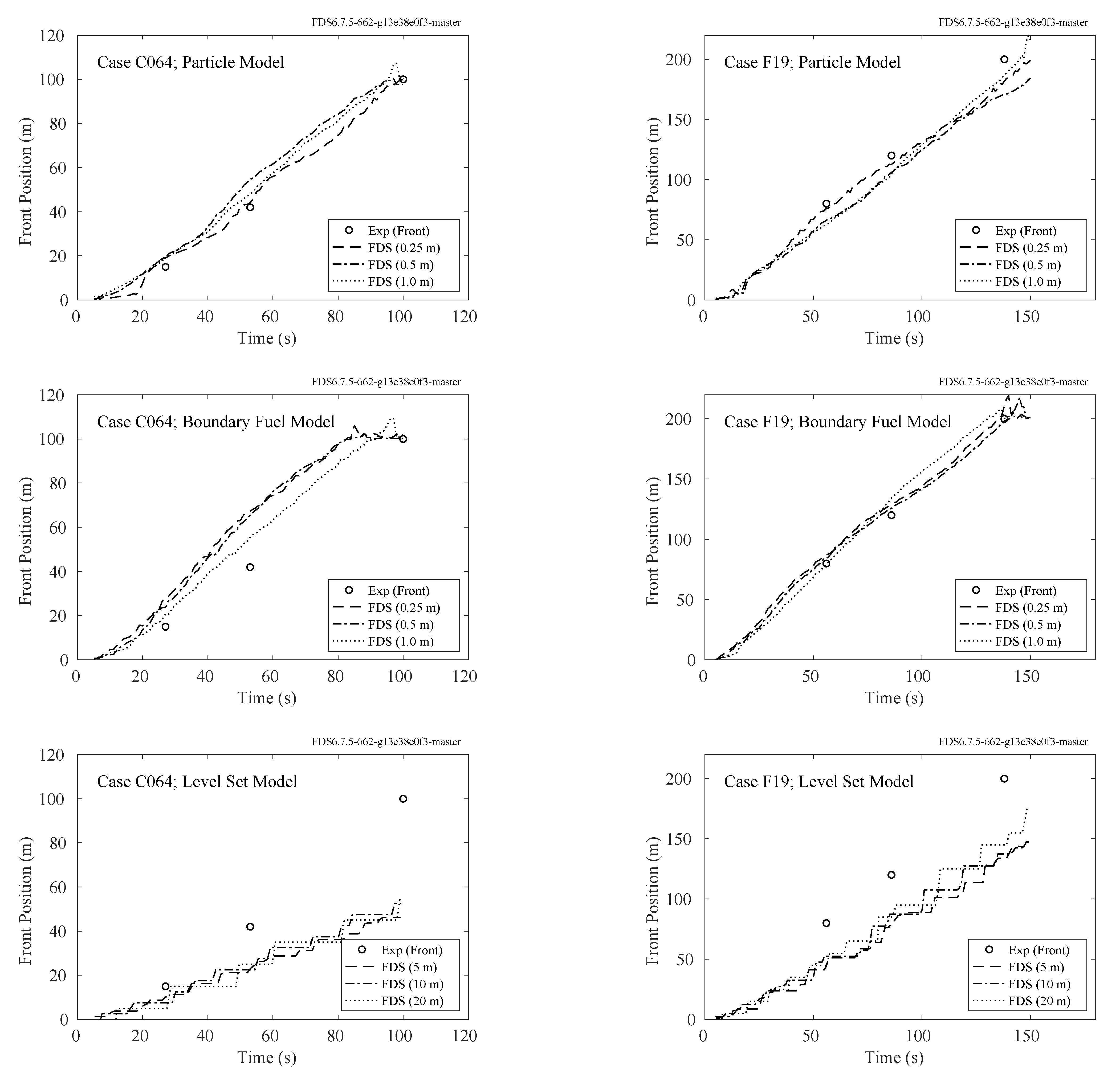
  • Particle Model: The vegetation (surface and raised) is represented by a collection of Lagrangian particles that are heated via convection and radiation. This model, with sufficient grid resolution, is appropriate for head, back, and flank surface fires, as well as fire through raised vegetation (e.g., trees). Heat transfer in the volume containing the vegetation is modeled in all three directions. This model is appropriate for grid resolutions of the order of 1 m or less, depending on the size of the flame base and properties of the vegetation (e.g., [49]).
  • Boundary Fuel Model: Surface vegetation has its own grid and is modeled like a porous solid with a thickness equal to the height of the vegetation. This model was designed for head fire spread in surface vegetation based on the assumption that heat transfer in the fuel bed is dominated by radiation from the overhead flame, and therefore in the vertical direction. In the implementation here, the height of the surface vegetation is assumed to be unresolved on the grid. The appropriate gas-phase grid resolution of the order is of 1 m to 10 m.
  • Level Set Method: The fire-front of a surface fire propagates using purely empirical rules in a level set method. Thermal degradation of the surface vegetation is not modeled. More than one implementation of this method is possible, largely differentiated by how the wind and fire-atmosphere interaction is modeled. The simpler implementations of this model can use grid resolutions that are coarser and 10 m or greater, than the more physics-based particle and boundary fuel models. The level set model can be used for fire spread in the surface vegetation, along with the particle model for fire behavior in raised vegetation.
The Particle Method and Boundary Fuel Model require thermo-physical properties of the vegetative fuels, and the fire spread rate is predicted by the model. The Level Set Method relies on a set of predetermined spread rates for different types of vegetation and wind speeds. The pyrolysis model, developed specifically for vegetation [50,51,52], consists of three reactions:
1. Endothermic moisture evaporation
Wet Vegetation ν H 2 O H 2 O + ( 1 ν H 2 O ) Dry Vegetation ; ν H 2 O = M 1 + M ;
2. Endothermic pyrolysis of dry vegetation
Dry Vegetation ν char Char + ( 1 ν char ) Fuel Gas ;
3. Exothermic char oxidation
Char + ν O 2 , char O 2 ( 1 + ν O 2 , char ν ash ) CO 2 + ν ash Ash .
M is the vegetation moisture content or moisture fraction determined on a dry weight basis. ν char is the mass fraction of dry vegetation that is converted to char during pyrolysis. ν O 2 , char is the mass of oxygen required per unit mass of char consumed. ν ash is the mass fraction of char that is converted to ash during char oxidation. Reaction rates and the various empirical kinetic constants are given in the References [50,51,52].

4.1. Particle Model

Lagrangian particles represent different types of vegetation, like leaves, grass, and pine needles. Each type of vegetation is represented by a single particle in each computational grid cell (multiple particles within a cell are permitted, but may not be the most computationally efficient approach). Most often, the particle is assumed to be cylindrical in shape, but it can be spherical or planar. The particle is assigned a diameter based on the measured surface area to volume ratio, σ . The length is relatively unimportant, so long as it is assumed to be much greater than the diameter. Material properties are assigned for the wet vegetation, which is assumed to dry out, decompose to char, and then exothermally oxidize when exposed to heat from an oncoming fire. The drag force exerted by the collection of particles is given by:
f b = ρ 2 C d C s β σ u u ,
where ρ is the air density, C d is the drag coefficient, C s is the shape factor (ratio of projected area to surface area), β is the packing ratio, σ is the surface area to volume ratio, and u is the air velocity. The diameter is specified via the surface area to volume ratio, and σ = 2 / r for a cylinder. The packing ratio is the volume of solid needles divided by the volume they occupy, typically denoted β . It is calculated by dividing the dry mass of vegetation per unit volume, the so-called “bulk density”, by the density of the dry vegetation, ρ d .
The drag coefficient for miscellaneous vegetation is taken to be 2.8, based on wind tunnel measurements [53]. The shape factor is assumed to be 0.25, which is the exact value for spheres and an approximate value for randomly oriented cylinders. In practice, the single term
κ = C s β σ
can be easier to determine than the three individual terms by measuring the relative amount of sunlight, W, that penetrates through a layer of vegetation of depth δ :
κ = ln W δ .
This value of κ also serves as the absorption coefficient for thermal radiation for a collection of particles.
The Lagrangian particles that represent vegetation are assumed to be thermally thick, but for simplicity, the heat conduction within the particle is assumed to be one-dimensional in either a cylindrical or spherical coordinate system. It is assumed that the particles interact with the surrounding gas via an additional source term in the energy conservation equation. For a grid cell with indices i j k , the source term is:
( · q ˙ r ) i j k = κ p U i j k 4 σ T p 4 ,
where T p is the particle surface temperature and the summation is over all the particles within the cell. The effective absorption coefficient for a single particle is given by
κ p = f A p 4 V = C s β σ ,
where A p is the surface area of the particle, V is the volume of the cell, and f is the number of actual particles represented by the single modeled particle. Notice that the absorption coefficient plays a role for both drag and radiation heat transfer.
The net radiative heat flux onto the surface of the particle is taken as:
q ˙ r = ϵ U i j k 4 σ T p 4 ,
where ϵ is the emissivity of the particle surface, typically assumed to be about 0.9. The convective heat transfer to the surface is given by:
q ˙ c = h ( T g T s ) ; h = k L Nu .
L is a characteristic length equal to the diameter of the sphere or cylinder. The Nusselt number is given by:
Nu = C 1 + C 2 Re n Pr m ; Re = ρ | u | L μ ; Pr = 0.7 .
For cylindrical particles, the default values are C 1 = 0 , C 2 = 0.683 , n = 0.466 , m = 0.33 , and L = D , the diameter of the cylinder. For spherical particles, the default values are C 1 = 2 , C 2 = 0.6 , n = 0.5 , m = 0.33 , and L = D , the diameter of the sphere [40].

4.2. Boundary Fuel Model

In many simulations of wildland fire, the surface vegetation layer is too shallow to be resolved explicitly, as is done when using Lagrangian particles to represent the vegetation. In such cases, the surface vegetation can be modeled as a porous boundary consisting of a layer of dry vegetation, moisture, and air, underneath which is hard ground [21]. The drag exerted by the vegetation is modeled using a special velocity boundary condition, and convective heat transfer is modeled via a source term in the one-dimensional heat conduction equation that is solved through the layer of vegetation and solid ground. Thermal radiation penetrates the vegetation layer via a 1D radiative transport equation that is used for semi-transparent solids.
The Boundary Fuel and Particle Models share the same basic input parameters and pyrolysis model. The drag exerted on the wind flowing through the vegetation is imposed as a force term in the gas phase grid cell adjacent to the boundary:
f b = ρ 2 C d C s β σ h b δ z u u ,
where the parameters are the same as in Equation (39) except for the additional depth of vegetation, h b , height of a grid cell, δ z , and u is the gas velocity in the first grid cell.
Thermal radiation is absorbed in depth according to a 1D radiative transport solver. The absorption coefficient is given by:
κ = C s σ β .
Thermal convection is not imposed at the interface between the gas phase and the vegetation layer, but rather imposed via a source term in the 1D heat conduction solver:
q ˙ c , b = σ β q ˙ c ,
where q ˙ c is given by Equation (45) and the gas velocity, | u | , and temperature, T g , are taken from the first gas phase grid cell adjacent to the boundary, and the particle surface temperature, T s , is extracted from the solution of the 1D heat conduction equation.

4.3. Level Set Model

For simulations of wildland fires spanning large areas that cannot be gridded finely enough to predict fire spread using the particle or boundary fuel models for vegetation, fire spread via a level approach is used [9]. It is assumed that a surface fire spreading from a point under certain wind, slope, and vegetation conditions does so with an ellipse-shaped fire front with, for an effective wind vector, a fixed length-to-breadth ratio [8,9]. Determining the spread rate vector at a point on the simulated fire front requires a formula for the magnitude of head fire rate of spread which is adjusted based on the location of the point on the idealized ellipse (e.g., head versus flank fire). This location is determined from the orientation of the effective wind vector relative to the normal to fire front represented by the level set.
The location of a fire front at time t is defined by the set of points x , y , where the level set scalar function ϕ ( x , y , t ) = 0 . The advection equation for the level set function is
D ϕ ( x , y , t ) D t = ϕ t + R u v · ( ϕ ) = 0 ,
where R u v = ( R u , R v ) is the spread rate vector.
As stated above, the magnitude of the spread rate vector on a point on the level set fire front is determined by adjusting the magnitude of the head fire spread rate. The direction of the spread rate vector is assumed to be normal to the fire front. A formula for magnitude of the head fire spread rate can be obtained a number of ways, including empirical models [54] and physics-based simulations [55]. A commonly used semi-empirical model is the Rothermel model [6,56], which can be implemented in FDS. Here, the magnitude of the head fire spread rate is
R u v   = R 0 1 + ( ϕ W + ϕ S ) · ( ϕ W + ϕ S ) ,
where R 0 is the zero-velocity, zero-slope rate of spread that depends on the fuel properties. The vectors ϕ W , ϕ S 0 are computed using the local wind and slope through empirical rules [57]. See Appendix 1 of Reference [9] for details on these calculations. The Rothermel model has been used in other CFD-based approaches, including the atmospheric weighted models WRF-SFIRE [17] and CAWFE [11].
In FDS, the level set spread model can be implemented in the following ways:
  • Only the level set simulation is performed, with a constant and uniform specified wind and slope. The wind is not affected by the terrain, and there is no fire.
  • The wind field is established over the terrain, but it is “frozen” when the fire ignites.
  • The wind field follows the terrain, but there is no actual fire in the simulation, just front-tracking. The level set evolves continuously in time with the flow field.
  • The wind and fire are fully coupled, and the resulting wind values are used in the head fire spread-rate formula. When the fire-front arrives at a given surface cell, it burns for a finite duration and with a heat release per unit area provided as part of the fuel model.
  • The wind and fire are fully coupled in the gas phase, but the head fire spread-rate is not influenced by the wind speed.
When fully coupled to the CFD model, the level set function acts as an igniter, as it reaches a new surface cell. The cell burns for a pre-determined amount of time. For cases where the depth of the fireline is less than the size of a grid cell, the burning time is extended, while the burning rate is decreased so as to maintain conservation of fuel mass.

5. Atmospheric Wind Boundary Conditions

For outdoor flows, FDS prescribes the wind field through special “open” boundary conditions on the exterior of the computational domain. The boundary conditions consist of three components:
(i)
The specified upstream wind field (vertical profile of streamwise velocity components) based on prescribed Monin-Obukhov parameters imposed on fluid elements entering the domain;
(ii)
Optional specification of upstream turbulence based on Jarrin’s synthetic eddy method [58] (which is possible with the code, but not utilized in the test cases within this paper); and
(iii)
Nonuniform and nonstationary Dirichlet pressure boundary values for the Poisson equation.
The following sections provide more detail on the implementation of the boundary profiles and the pressure boundary conditions.

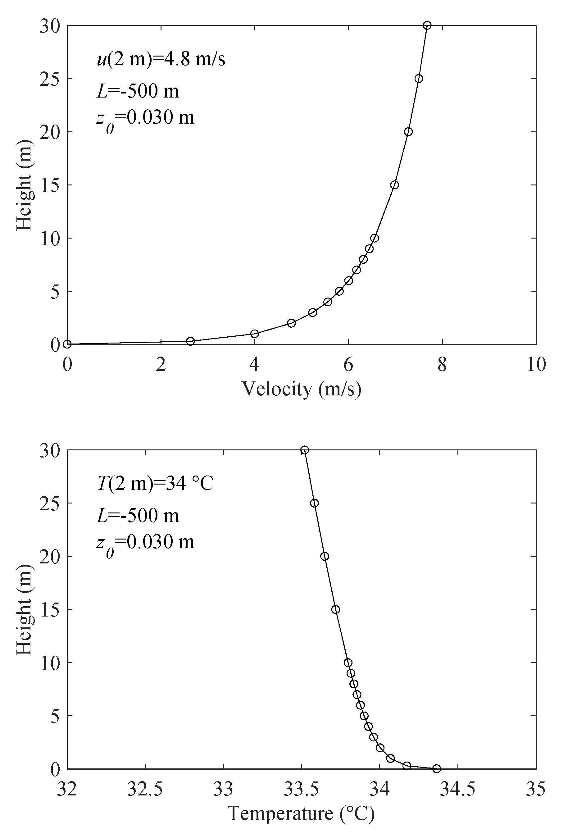
5.1. Velocity and Temperature Profiles

While completely custom vertical boundary profiles of velocity and temperature are possible, the wind field is usually specified via Monin–Obukhov (MO) similarity parameters [59]: Obukhov length scale, L, aerodynamic roughness height, z 0 , wind speed, u r , and temperature, T r , at a reference height z r . For a given set of MO parameters, FDS generates velocity and temperature profiles as functions of height, as shown in Figure 3. These values are specified for any fluid elements entering the domain at height z, including along the top of the domain. Convective outflow boundaries are applied locally for any fluid elements leaving the domain. The profiles can vary in time allowing one-way “downscaling” from either weather observations or output from a numerical weather prediction (NWP) model. However, two-way coupling with an NWP model (e.g., [14,60]) has not yet been implemented with FDS.

5.2. Pressure Boundary Values

The Poisson equation for H, Equation (33), links the momentum equation with mass and energy in the low-Mach flow algorithm. The boundary conditions for this equation determine the inflow and outflow velocity component values. Let n denote a unit normal vector pointing into the domain. Boundary values at an interface are denoted with a subscript “I”. Then, u I · n > 0 is an inflow, and u I · n < 0 is an outflow condition.
At an inflow, the mean viscous and convective forces are generally small, and a simplified momentum equation may be used to develop a boundary value for H, namely, u i / t = H / x i . To develop the boundary condition, let u denote the x-component of velocity and consider an interface normal to x pointing into the domain. The prescribed external wind field velocity component at height z and time t (discussed above in Section 5.1) is denoted u w i n d ( z , t ) . Using a one-sided difference for H and an explicit Euler approximation of the velocity time derivative, the boundary value for H may be written as
H I = H I ± 1 2 n ± Δ x 2 u w i n d , I ( z , t ) u I n Δ t if u I · n > 0 .
At an outflow boundary, H is set equal to the local kinetic energy per unit mass from the cell just upwind of the boundary:
H I = 1 2 ( u ¯ n u ¯ n + v ¯ n v ¯ n + w ¯ n w ¯ n ) I ± 1 2 if u I · n 0 .
The overbar on the velocity components denotes a linear interpolation of the primitive staggered component values to the cell center.

6. Numerical Experiments

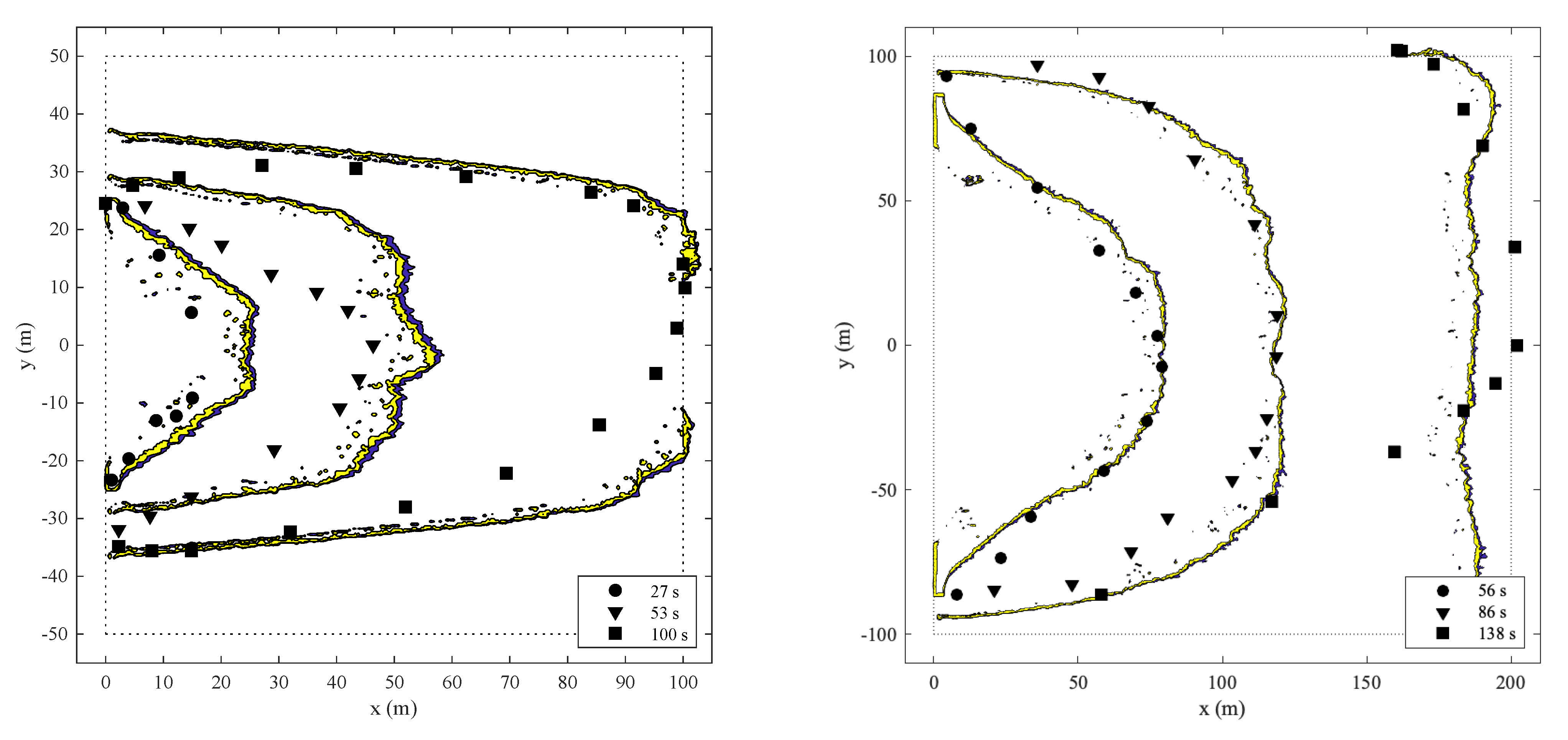
6.1. Flat Terrain Fire Spread

In July and August of 1986, the Commonwealth Scientific and Industrial Research Organisation (CSIRO) of Australia conducted controlled grassland fire experiments near Darwin, Northern Territory [61]. July and August are in the middle of the dry season when the grasses are fully cured (dried) and the weather is warm and dry. The experiments were conducted on flat plots measuring 100 m by 100 m, 200 m by 200 m, or 200 m by 300 m. Two cases have been simulated. Case C064 was conducted on a 100 m by 100 m plot of kerosene grass (Eriachne burkittii); Case F19 was conducted on a 200 m by 200 m plot of kangaroo grass (Themeda australis).
Two of these experiments were originally simulated with FDS by Mell et al. [21] using a form of the Boundary Fuel Model. Now these two experiments are also simulated using the Lagrangian Particle Model and the Level Set Model. The level set simulations of Case C064 use fuel index 1 (Short Grass) and for Case F19, fuel index 3 (Tall Grass) [6,56].
Measured bulk properties of the grasses burned in the two experiments are listed in Table 1. Properties that were not measured are listed in Table 2. These assumed properties are typically for wood or cellulosic fuels. The moisture is modeled as water. The grass is assumed to be composed primarily of cellulose.
Snapshots of the Lagrangian particle simulation of Case F19 compared to photographs of the experiment are shown in Figure 4. The plot of grass is 200 m by 200 m, and the computational domain is 240 m by 240 m by 20 m high. The grid cells are 0.5 m cubes. The domain is subdivided into 36 individual meshes and run in parallel. A blade of grass is represented by a single cylindrically shaped particle within a grid cell. The radius of the cylinder is derived from the measured surface area to volume ratio of the grass. Each simulated blade of grass represents many more actual blades of grass. The weighting factor is determined from the measured bulk mass per unit area. The fires in the experiments were ignited by two field workers carrying drip torches walking in opposite directions along the upwind boundary of the plot (the red strip in Figure 4). In FDS, this action was modeled using a specified spread rate along the strip.
The simulations were conducted with the three different fire spread models, and each case was run with three levels of spatial resolution. The simulations using the Particle and Boundary Fuel Models were run with cubic grid cells that were 0.25 m, 0.5 m, and 1 m on a side. The simulations using the Level Set Model were run with cells of 5 m, 10 m, and 20 m. The predicted rates of spread for the two cases are listed in Table 1 and shown graphically in Figure 5. For these simulations, the rate of spread predicted by the Particle and Boundary Fuel Models are comparable to the measured rate of spread, while the level set method under-predicts the RoS. The under-prediction by the level set simulations is a consequence of the limitations of the Rothermel model, which is based on empirical relations largely derived from laboratory-scale experiments. It is well-known that practical application of the Rothermel model often requires calibration for the case of interest [62]. The use of the Rothermel for the head fire spread rate in surface vegetation in FDS is to be viewed as a placeholder that is in-line with other CFD-based models. If the observed head fire rate of spread for the F19 and C064 experiments is used in FDS, then good agreement with the observed fire perimeter is obtained (not shown). Further work is needed to develop rate-of-spread models appropriate for use with the Level Set Model (e.g., [55]).
Figure 6 shows contours of heat release rates near the surface compared to the observed flame front for the high-resolution (0.25 m) Particle Model. These contours may be compared to the head fire spread rates at the top of Figure 5. Case F19 contours are shown on the right, and may be compared to the flame images in Figure 4. These results show some improvement to the flank fire spread rates compared to previous simulations with FDS conducted by Mell et al. in 2007 [21].
However, it is difficult to compare the present results with those from [21]. The underlying numerical model, FDS, has undergone a major revision over the past decade, changing the basic finite-difference scheme, boundary conditions, drag modeling, and so on, and the vegetation-specific models have changed as well, most notably the charring reaction. In addition, the amount of information about the grasses and field conditions is limited, and the thermal and kinetic parameters gleaned from various sources are generally average values over a wide range of vegetation types. A sensitivity study [66] for the particle model simulations reveals that near-surface wind speed has the most direct effect on the rate of spread (RoS), and the combined effect of the dozens of thermal, kinetic, and numerical parameters would certainly explain the difference in RoS between the 2007 results and those of this study.

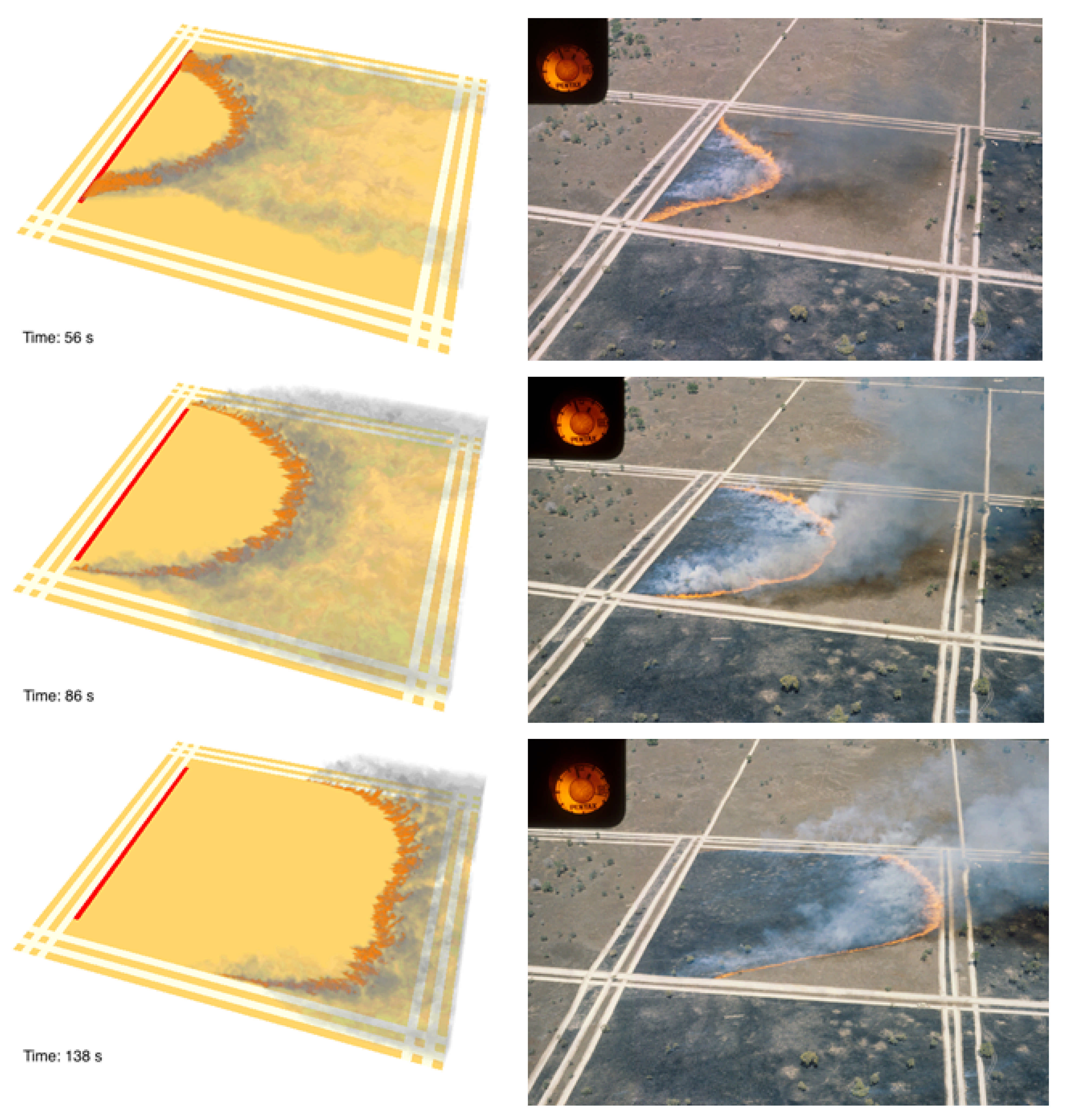
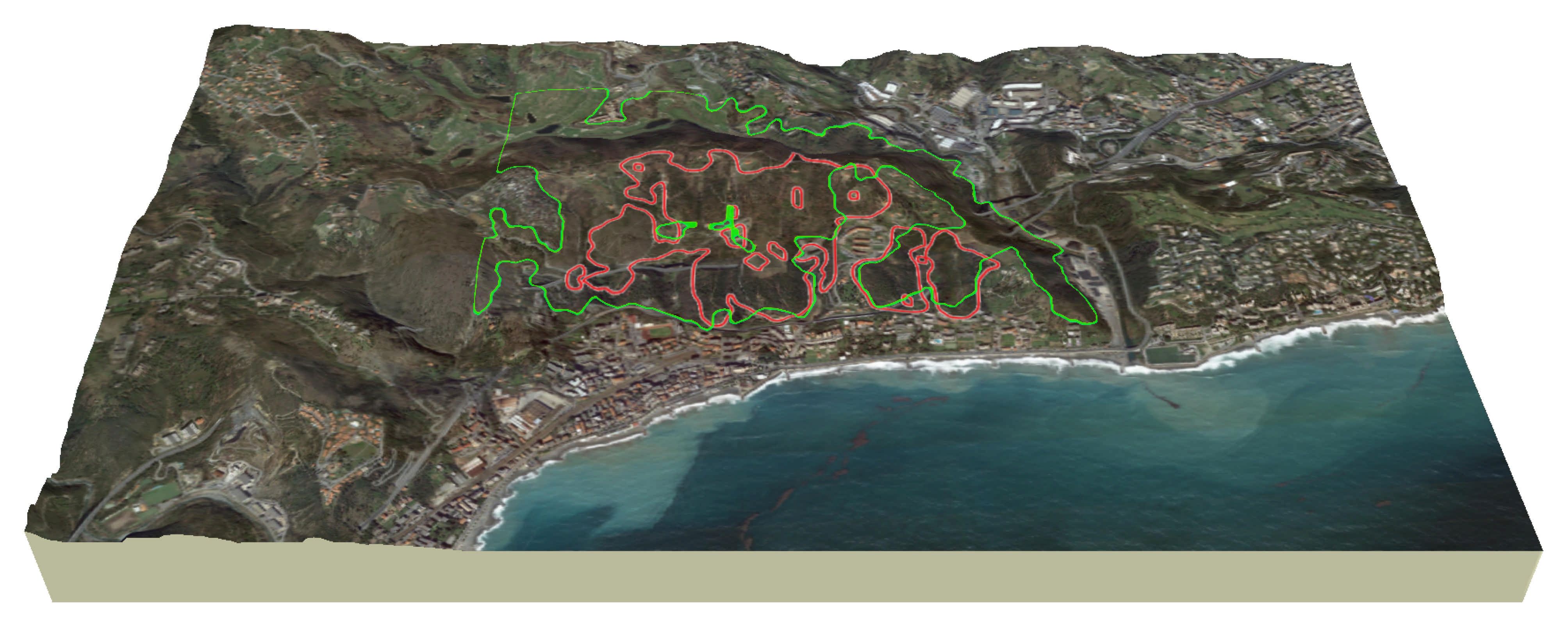
6.2. Complex Terrain Fire Spread

This section presents an example of the methodologies discussed in the paper. It is notable because it considers an actual fire that occurred in the wildland–urban interface (WUI), which presents a challenge for a fire spread model because the surface vegetation is mixed with the built environment.
At approximately 23:00 (local time) on 25 March 2019, a wildfire started in the seaside town of Cogoleto, near Genoa, Italy. Strong winds, gusting up to 100 km/h from the north, spread the fire from its ignition point towards the sea. The fire was caused by a faulty power line on a ridge above the town. Several houses were destroyed, and hundreds of residents had to be evacuated. The burnt region measured over 1 km from the origin to the farthest point. The fire burned overnight and into the next day. Up to 70 firefighters worked at the scene, with help from helicopters and fire hydrants. Suppression efforts were directed towards stopping the fire spread into the coastal town of Cogoleto.
Shown in Figure 7 are the results of a level set simulation of the fire superimposed on a satellite photograph of the area and the outline of the extent of the actual fire. The computational domain was assembled using an open-source, Geographic Information System (GIS) program called QGIS [67], extended by the qgis2fds [68] plugin. The open-source qgis2fds plugin was specifically developed in the framework of the WUIFI-21 project for facilitating the use of geographical data for forest fire simulation and smoke pollutants dispersion in FDS (WUIFI-21: High-fidelity computational fluid dynamics modeling of forest fires for wildland–urban Interface communities resilience and protection is an Italy–US research project financed by the Italian Ministry of Foreign Affairs and International Cooperation).
The wind speed and direction are based on a single weather station near the point of ignition. Winds recorded were found to be predominantly coming from the north, with magnitudes that ranged from 20 m/s during the night and diminishing to 5 m/s towards the morning hours. The vegetation type was provided by a database maintained at the International Centre on Environmental Monitoring (CIMA) Research Foundation, derived from regional forest management maps. In the simulation, the single-point wind data were taken as the prevailing wind, and the local wind field was obtained via CFD computation. The fire was simulated based on the position of the level set front; that is, when the front arrived at a given location, a fire was ignited and burned for a duration of time consistent with the specified fuel loading of that particular point on the map.
The extent of the simulated fire, shown in green in Figure 7, is greater than that of the actual fire, shown in red. This is not surprising, given that the simulation does not include suppression and the rate of spread of the level set front is determined based on vegetation that may not exactly resemble that of this particular region. It is important to note that for the level set method, a fire break created by first responders can be modeled as a region declared as “non-combustible”. The 13 Rothermel fuel types have been supplemented by areas such as water, pavement, and other non-combustibles. The fire-front determined by the level set calculation is stopped by the non-combustible area, highlighting the challenge in simulating firebrand spot ignitions that were reported by first responders at the scene.
The simulation results have been compared with those obtained from the CIMA Propagator [69], an experimental propagation model that has provided several European civil protection organizations with real-time fire predictions since 2009. The model has been implemented by the CIMA Foundation, and its propagation model is based on stochastic cellular automata.
The two models produce a qualitatively similar patterns of fire spread, mainly because the vicinity of the fire has numerous areas that are considered “non-combustible”, that is, devoid of vegetation or structures. This points out the problem of “validating” wildfire models. The simulations of the flat terrain grassland fire experiments described in the previous section match the observed fire behavior fairly well, but in those cases, the vegetation is uniform and fairly well-described in terms of its mass loading and geometrical characteristics, the terrain is flat and of relatively small area, the wind is steady, and the experiment lasts a few minutes. In a real fire, none of this will be true. The detailed physics of the fire are not resolvable on a relatively coarse grid, the vegetation is heterogeneous, sparse, and sometimes unknown, the weather conditions are varying, there are suppression efforts with water and the setting of backfires, and the fires can burn for days.
All of this raises the question as to what level of physical fidelity ought to be required in these models. The strategy that has been adopted in FDS is to accommodate simulation options ranging from a level set calculation of fire spread over tens of kilometers that can be run in minutes, similar to models like FARSITE developed by the US Forest Service, all the way to detailed simulations of fire spread at sub-meter resolution for relatively short time-periods (minutes to hours) and small areas (tens of hectares). As was the case for models developed for building fires 30 years ago, it is not clear at the moment exactly how these wildland fire models will be used in the future. The best strategy is to advance the various modeling options until a clear path forward becomes apparent.

7. Summary

The numerical methods described in this paper span the range of length scales from tens of centimeters to tens of kilometers. Obviously, these techniques support differing descriptions of the underlying fire physics, but all can be embedded within the same code base. This allows researchers to combine the different techniques in ways that were not possible when separate codes were maintained by separate organizations. With FDS, one can simulate 24 h of fire spread in minutes of computation time using the level set function and a wind field that varies only temporally, not spatially, with no fire–atmospheric coupling. At the same time, using the same set of input parameters, one can simulate the fire at far greater resolutions with much greater physical fidelity, albeit for shorter time-periods and spatial extent.

Author Contributions

Conceptualization, M.V.; Data curation, R.M.; Investigation, K.M. and W.M.; Software, E.G. and P.F.; Visualization, G.F. All authors have read and agreed to the published version of the manuscript.

Funding

This work was partially funded by the Risk Reduction in Communities Program at NIST. W.M. acknowledges support from the Strategic Environmental Research and Development Program (SERDP) Grant RC19-1132.

Data Availability Statement

The Fire Dynamics Simulator is an open-source computational fluids dynamics code available at https://github.com/firemodels/fds. The input files for the CSIRO wildfire spread calculations are also kept within this repository.

Conflicts of Interest

The authors declare no conflict of interest.

References

  1. Thomas, D.; Butry, D.; Gilbert, S.; Webb, D.; Fung, J. The Costs and Losses of Wildfires: A Literature Review; Special Publication NIST SP-1215; National Institute of Standards and Technology: Gaithersburg, MD, USA, 2017. Available online: https://www.nist.gov/publications/costs-and-losses-wildfires (accessed on 5 February 2021).
  2. McDermott, R.; Bryner, N.; Heintz, J. Large Outdoor Fire Modeling (LOFM) Workshop Summary Report; Special Publication NIST SP-1245; National Institute of Standards and Technology: Gaithersburg, MD, USA, 2019. Available online: https://www.nist.gov/publications/large-outdoor-fire-modeling-lofm-workshop-summary-report (accessed on 5 February 2021).
  3. Richards, L.; Brew, N.; Smith, L. 2019–20 Australian Bushfires—Frequently Asked Questions: A Quick Guide; Research Paper Series 2019-20; Parliament of Australia: Canberra, Australia, 2020. Available online: https://parlinfo.aph.gov.au/parlInfo/download/library/prspub/7234762/upload_binary/7234762.pdf (accessed on 5 February 2021).
  4. Papadopoulos, G.D.; Niovi Pavlidou, F. A Comparative Review on Wildfire Simulators. IEEE Syst. J. 2011, 5, 233–243. [Google Scholar] [CrossRef]
  5. Bakhshaii, A.; Johnson, E. A review of a new generation of wildfire–atmosphere modeling. Can. J. For. Res. 2019, 49, 565–574. [Google Scholar] [CrossRef] [Green Version]
  6. Rothermel, R.C. A Mathematical Model for Predicting Fire Spread in Wildland Fuels; Technical Report INT-115; USDA Forest Service: Ogden, UT, USA, 1972. Available online: http://www.treesearch.fs.fed.us/pubs/32533 (accessed on 5 February 2021).
  7. Anderson, H. Aids to Determining Fuel Models for Estimating Fire Behavior; General Technical Report INT-122; Intermountain Forest and Range Experiment Station, USDA Forest Service: Ogden, UT, USA, 1982. Available online: https://www.fs.usda.gov/treesearch/pubs/6447 (accessed on 5 February 2021).
  8. Finney, M. Fire Area Simulator–Model, Development and Evaluation; Research Paper RMRS-RP-4 Revised; United States Forest Service, Rocky Mountain Research Station: Missoula, MT, USA, 2004. Available online: http://www.fs.fed.us/rm/pubs/rmrs_rp004.pdf (accessed on 5 February 2021).
  9. Bova, A.; Mell, W.; Hoffman, C. A comparison of level set and marker methods for the simulation of wildland fire front propagation. Int. J. Wildland Fire 2015, 25, 229–241. [Google Scholar] [CrossRef]
  10. McGrattan, K.; Hostikka, S.; McDermott, R.; Floyd, J.; Weinschenk, C.; Overholt, K. Fire Dynamics Simulator, User’s Guide, 6th ed.; National Institute of Standards and Technology: Gaithersburg, MD, USA; VTT Technical Research Centre of Finland: Espoo, Finland, 2013. [Google Scholar]
  11. Coen, J.L. Modeling Wildland Fires: A Description of the Coupled Atmosphere-Wildland Fire Environment Model (CAWFE); Technical Report NCAR/TN500+STR; National Center for Atmospheric Research: Boulder, CO, USA, 2013. [Google Scholar]
  12. Coen, J.L.; Schroeder, W. The High Park Fire: Coupled weather-wildland fire model simulation of a windstorm-driven wildfire in Colorado’s Front Range. J. Geophys. Res. Atmos. 2015, 120, 131–146. [Google Scholar] [CrossRef]
  13. Lautenberger, C. Wildland fire modeling with an Eulerian level set method and automated calibration. Fire Saf. J. 2013, 62, 289–298. [Google Scholar] [CrossRef]
  14. Coen, J.L.; Cameron, M.; Michalakes, J.; Patton, E.G.; Riggan, P.J.; Yedinak, K.M. WRF-Fire: Coupled Weather—Wildland Fire Modeling with the Weather Research and Forecasting Model. J. Appl. Meteorol. Climatol. 2013, 52, 16–38. [Google Scholar] [CrossRef]
  15. Mandel, J.; Beezley, J.D.; Coen, J.L.; Kim, M. Data assimilation for wildland fires: Ensemble Kalman filters in coupled atmosphere-surface models. IEEE Control Syst. Mag. 2009, 9, 47–65. [Google Scholar]
  16. Mandel, J.; Beezley, J.D.; Kochanski, A.K. Coupled atmosphere-wildland fire modeling with WRF 3.3 and SFIRE 2011. Geosci. Model Dev. 2011, 4, 591–610. [Google Scholar] [CrossRef] [Green Version]
  17. Mandel, J.; Amram, S.; Beezley, J.D.; Kelman, G.; Kochanski, A.K.; Kondratenko, V.Y.; Lynn, B.H.; Regev, B.; Vejmelka, M. Recent advances and applications of WRF-SFIRE. Nat. Hazards Earth Syst. Sci. 2015, 14, 2829–2845. [Google Scholar] [CrossRef] [Green Version]
  18. Kochanski, A.K.; Jenkins, M.A.; Yedinak, K.; Mandel, J.; Beezley, J.; Lamb, B. Toward an integrated system for fire, smoke, and air quality simulations. Int. J. Wildland Fire 2016, 25, 534–546. [Google Scholar] [CrossRef] [Green Version]
  19. Sethian, J.A. Level Set Methods and Fast Marching Methods: Evolving Interfaces in Computational Geometry, Fluid Mechanics, Computer Vision, and Materials Science; Cambridge University Press: Cambridge, UK, 1999. [Google Scholar]
  20. Osher, S.; Fedkiw, R. Level Set Methods and Dynamic Implicit Surfaces; Springer: Berlin/Heidelberg, Germany, 2006. [Google Scholar]
  21. Mell, W.; Jenkins, M.; Gould, J.; Cheney, P. A physics-based approach to modelling grassland fires. Int. J. Wildland Fire 2007, 16, 1–22. [Google Scholar] [CrossRef]
  22. Linn, R.; Winterkamp, J.; Edminster, C.; Colman, J.J.; Smith, W.S. Coupled influences of topography and wind on wildland fire behaviour. Int. J. Wildland Fire 2007, 16, 183–195. [Google Scholar] [CrossRef]
  23. Arca, B.; Ghisu, T.; Casula, M.; Salis, M.; Duce, P. A web-based wildfire simulator for operational applications. Int. J. Wildland Fire 2019, 28, 99–112. [Google Scholar] [CrossRef]
  24. Rehm, R.; Baum, H. The Equations of Motion for Thermally Driven, Buoyant Flows. J. Res. NBS 1978, 83, 297–308. [Google Scholar] [CrossRef]
  25. McDermott, R.; Floyd, J. Enforcing realizability in explicit multi-component species transport. Fire Saf. J. 2015, 78, 180–187. [Google Scholar] [CrossRef] [PubMed] [Green Version]
  26. McDermott, R.J. A velocity divergence constraint for large-eddy simulation of low-Mach flows. J. Comput. Phys. 2014, 274, 413–431. [Google Scholar] [CrossRef]
  27. Pope, S.B. Turbulent Flows; Cambridge University Press: Cambridge, UK, 2000. [Google Scholar]
  28. McGrattan, K.; Hostikka, S.; McDermott, R.; Floyd, J.; Weinschenk, C.; Overholt, K. Fire Dynamics Simulator, Technical Reference Guide, 6th ed.; Volume 1: Mathematical Model; Volume 2: Verification Guide; Volume 3: Validation Guide; Volume 4: Software Quality Assurance; National Institute of Standards and Technology: Gaithersburg, MD, USA; VTT Technical Research Centre of Finland: Espoo, Finland, 2013. [Google Scholar]
  29. Poinsot, T.; Veynante, D. Theoretical and Numerical Combustion, 2nd ed.; R.T. Edwards, Inc.: Philadelphia, PA, USA, 2005. [Google Scholar]
  30. Deardorff, J. Stratocumulus-capped mixed layers derived from a three-dimensional model. Boundary-Layer Meteorol. 1980, 18, 495–527. [Google Scholar] [CrossRef]
  31. Comte-Bellot, G.; Corrsin, S. Simple Eulerian time correlation of full- and narrow-band velocity signals in grid-generated, ‘isotropic’ turbulence. J. Fluid Mech. 1971, 48, 273–337. [Google Scholar] [CrossRef]
  32. Bardina, J.; Ferziger, J.H.; Reynolds, W.C. Improved Subgrid Scale Models for Large Eddy Simulation. In Proceedings of the AIAA 13th Fluid & Plasma Dynamics Conference, American Institute of Aeronautics and Astronautics, Snowmass, CO, USA, 14–16 July 1980. [Google Scholar]
  33. Nicoud, F.; Ducros, F. Subgrid-Scale Stress Modelling Based on the Square of the Velocity Gradient Tensor. Flow Turbul. Combust. 1999, 62, 183–200. [Google Scholar] [CrossRef]
  34. Maragkos, G.; Merci, B. On the use of dynamic turbulence modelling in fire applications. Comb. Flame 2020, 216, 9–23. [Google Scholar] [CrossRef]
  35. Mulholland, G. Smoke Production and Properties. In SFPE Handbook of Fire Protection Engineering, 3rd ed.; National Fire Protection Association: Quincy, MA, USA, 2002. [Google Scholar]
  36. Magnussen, B.; Hjertager, B. On Mathematical Modeling of Turbulent Combustion with Special Emphasis on Soot Formation and Combustion. In Proceedings of the Sixteenth Symposium (International) on Combustion, Combustion Institute, Pittsburgh, PA, USA, 15–20 August 1976; pp. 719–729. [Google Scholar]
  37. McDermott, R.; McGrattan, K.; Floyd, J. A Simple Reaction Time Scale for Under-Resolved Fire Dynamics. In Proceedings of the Fire Safety Science—10th International Symposium, College Park, MD, USA, 19–24 June 2011; pp. 809–820. [Google Scholar]
  38. Beyler, C. Flammability Limits of Premixed and Diffusion Flames. In SFPE Handbook of Fire Protection Engineering, 5th ed.; Hurley, M., Ed.; Springer: New York, NY, USA, 2016. [Google Scholar]
  39. Holman, J. Heat Transfer, 7th ed.; McGraw-Hill: New York, NY, USA, 1990. [Google Scholar]
  40. Incropera, F.P.; De Witt, D.P. Fundamentals of Heat and Mass Transfer, 4th ed.; John Wiley and Sons: New York, NY, USA, 1996. [Google Scholar]
  41. Berger, M. Cut Cells: Meshes and Solvers. Handb. Numer. Anal. 2017, 18, 1–22. [Google Scholar]
  42. Eymard, R.; Gallouet, T.; Herbin, R. Finite volume methods. In Solution of Equation in Rn (Part 3), Techniques of Scientific Computing (Part 3); Handbook of Numerical Analysis; Elsevier: Amsterdam, The Netherlands, 2000; Volume 7, pp. 713–1018. [Google Scholar]
  43. LeVeque, R. Finite Volume Methods for Hyperbolic Problems; Cambridge Texts in Applied Mathematics; Cambridge University Press: Cambridge, UK, 2002. [Google Scholar]
  44. Balaras, E. Modeling complex boundaries using an external force field on fixed Cartesian grids in large-eddy simulations. Comput. Fluids 2004, 33, 375–404. [Google Scholar] [CrossRef]
  45. LeVeque, R. Finite Difference Methods for Ordinary and Partial Differential Equations: Steady-State and Time-Dependent Problems; Other Titles in Applied Mathematics; Society for Industrial and Applied Mathematics: Philadelphia, PA, USA, 2007. [Google Scholar]
  46. Kirkpatrick, M.; Armfield, S.; Kent, J. A representation of curved boundaries for the solution of the Navier–Stokes equations on a staggered three-dimensional Cartesian grid. J. Comput. Phys. 2003, 184, 1–36. [Google Scholar] [CrossRef]
  47. Perot, J. An Analysis of the Fractional Step Method. J. Comput. Phys. 1993, 108, 51–58. [Google Scholar] [CrossRef]
  48. Fadlun, E.; Verzicco, R.; Orlandi, P.; Mohd-Yusof, J. Combined Immersed-Boundary Finite-Difference Methods for Three-Dimensional Complex Flow Simulations. J. Comput. Phys. 2000, 161, 35–60. [Google Scholar] [CrossRef]
  49. Perez-Ramirez, Y.; Santoni, P.; Tramoni, J.; Bosseur, F.; Mell, W. Examination of WFDS in Modeling Spreading Fires in a Furniture Calorimeter. Fire Technol. 2017, 53, 1795–1832. [Google Scholar] [CrossRef]
  50. Porterie, B.; Consalvi, J.; Kaiss, A.; Loraud, J. Predicting Wildland Fire Behavior and Emissions Using a Fine-Scale Physical Model. Numer. Heat Transf. Part A 2005, 47, 571–591. [Google Scholar] [CrossRef]
  51. Morvan, D.; Dupuy, J. Modeling the propagation of a wildfire through a Mediterranean shrub using a multiphase formulation. Combust. Flame 2004, 138, 199–210. [Google Scholar] [CrossRef]
  52. Houssami, M.; Mueller, E.; Filkov, A.; Thomas, J.; Skowronski, N.; Gallagher, M.; Clark, K.; Kremens, R.; Simeoni, A. Experimental procedures characterizing firebrand generation in wildland fires. Fire Technol. 2016, 52, 731–751. [Google Scholar] [CrossRef]
  53. Falkenstein-Smith, R.; McGrattan, K.; Toman, B.; Fernandez, M. Measurement of the Flow Resistance of Vegetation; NIST Technical Note 2039; National Institute of Standards and Technology: Gaithersburg, MD, USA, 2019; Available online: https://doi.org/10.6028/NIST.TN.2039 (accessed on 5 February 2021).
  54. Cheney, N.; Gould, J.; Catchpole, W. Predition of Fire-Spread in Grasslands. Int. J. Wildland Fire 1993, 8, 1–13. [Google Scholar] [CrossRef]
  55. Mell, W.; Hoffman, C.; Ziegler, J. The state of physics-based fire modeling and an example of a reduced fire-physics model. In Proceedings of the 6th International Fire Behavior and Fuels Conference, International Association of Wildland Fire, Missoula, MT, USA, 29 April–3 May 2019. [Google Scholar]
  56. Albini, F. Estimating Wildfire Behavior and Effects; Research Paper INT-30; Intermountain Forest and Range Experiment Station, USDA Forest Service: Ogden, UT, USA, 1976; Available online: https://www.fs.fed.us/rm/pubs_int/int_gtr030.pdf (accessed on 5 February 2021).
  57. Wilson, R. Reformulation of Forest Fire Spread Equations in SI Units; Research Note INT-292; Intermountain Forest and Range Experiment Station, USDA Forest Service: Ogden, UT, USA, 1980. Available online: https://www.fs.usda.gov/treesearch/pubs/33592 (accessed on 5 February 2021).
  58. Jarrin, N. Synthetic Inflow Boundary Conditions for the Numerical Simulation of Turbulence. Ph.D. Thesis, The University of Manchester, Manchester, UK, 2008. [Google Scholar]
  59. Dyer, A. A review of flux profile relationships. Boundary-Layer Meteorol. 1974, 7, 363–372. [Google Scholar] [CrossRef]
  60. Coupled Atmosphere-Wildland Fire Environmant (CAWFE); National Center for Atmospheric Research: Boulder, CO, USA, 2013.
  61. Cheney, N.; Gould, J.; Catchpole, W. The Influence of Fuel, Weather and Fire Shape Variables on Fire-Spread in Grasslands. Int. J. Wildland Fire 1993, 3, 31–44. [Google Scholar] [CrossRef]
  62. Arca, B.; Duce, P.; Laconi, M.; Pellizzaro, G.; Salis, M.; Spano, D. Evaluation of FARSITE simulator Mediterranean marquis. Int. J. Wildland Fire 2007, 16, 563–573. [Google Scholar] [CrossRef]
  63. Susott, R. Characterization of the thermal properties of forest fuels by combustible gas analysis. For. Sci. 1982, 2, 404–420. [Google Scholar]
  64. Khan, M.; Tewarson, A.; Chaos, M. Combustion Characteristics of Materials and Generation of Fire Products. In SFPE Handbook of Fire Protection Engineering, 5th ed.; Springer: New York, NY, USA, 2016; Chapter 36; pp. 1143–1232. [Google Scholar]
  65. Farouki, O. Thermal Properties of Soils; CRREL Monograph 81-1; U.S. Army Corps of Engineers, Cold Regions Research and Engineering Laboratory: Hanover, NH, USA, 1981. [Google Scholar]
  66. McGrattan, K. Progress in Modeling Wildland Fires using Computational Fluid Dynamics. In Proceedings of the 10th U.S. National Combustion Meeting, College Park, MD, USA, 23–26 April 2017. [Google Scholar]
  67. Available online: https://qgis.org/en/site/ (accessed on 5 February 2021).
  68. Available online: https://github.com/firetools/qgis2fds/wiki/ (accessed on 5 February 2021).
  69. Trucchia, A.; D’Andrea, M.; Baghino, F.; Fiorucci, P.; Ferraris, L.; Negro, D.; Gollini, A.; Severino, M. PROPAGATOR: An Operational Cellular-Automata Based Wildfire Simulator. Fire 2020, 3, 26. [Google Scholar] [CrossRef]
Figure 1. Sketch of regular Cartesian and cut-cell grids around terrain: (a) An unstructured cut-cell region is defined on the gas phase side around a terrain T . (b) Detail showing a slice representative of cut-cells and regular gas cells, terrain triangulation, and two level refinement interpretations.
Atmosphere 12 00273 g001
Figure 2. Sketch of cut-cell and faces: (a) Cut-cell i i surrounded by gas phase regular and cut-faces (3–5), and boundary cut-faces (1–2). (b) Interpolation sketch for wall-modeled, immersed boundary reconstruction of cut-face velocities.
Atmosphere 12 00273 g002
Figure 3. Monin–Obukhov velocity and temperature profiles for inflow boundary conditions. Here, parameters are L = 500 m , z 0 = 0.03 m , and u r = 4.8 m / s and T r = 34 C .
Atmosphere 12 00273 g003
Figure 4. Photographs of the experiment and snapshots of the simulation (medium resolution Particle Model) of CSIRO Grassland Fire F19, 56 s, 86 s, and 138 s following ignition.
Atmosphere 12 00273 g004
Figure 5. Comparison of the measured and predicted fire front position for the CSIRO Grassland Fires using three different methods of fire spread.
Atmosphere 12 00273 g005
Figure 6. Contours of heat release rate in a plane near the surface from the fine resolution (0.25 m) Particle Model compared to observations of CSIRO Grassland Fires C064 (left) and F19 (right).
Atmosphere 12 00273 g006
Figure 7. Satellite photograph of the region where the Cogoleto Fire occurred. The area outlined in red is the extent of the actual fire; green is the simulation.
Atmosphere 12 00273 g007
Table 1. Measured properties for the CSIRO Grassland Fire cases [61].
PropertyUnitsCase C064Case F19
Wind Speedm/s4.64.8
Ambient Temperature C3234
Surface Area to Volume Ratiom 1 977012,240
Grass Heightm0.210.51
Bulk Mass per Unit Areakg/m 2 0.2830.313
Moisture Fraction%6.35.8
Measured RoSm/s1.21.5
Calc’d RoS, Particle Method (0.25 m, 0.5 m, 1.0 m resolution)m/s1.1, 1.2, 1.21.4, 1.3, 1.4
Calc’d RoS, Boundary Fuel Method (0.25 m, 0.5 m, 1.0 m resolution)m/s1.3, 1.3, 1.31.5, 1.4, 1.7
Calc’d RoS, Level Set Method (5 m, 10 m, 20 m resolution)m/s0.5, 0.6, 0.61.0, 1.1, 1.2
Table 2. Assumed properties for various types of dried grass and soil. Note that the Pyrolysis Temperature is taken to be the temperature at which the mass loss rate peaks in the TGA experiments of Morvan and Dupuy [51].
PropertyUnitsValueReference
Chemical CompositionC 6 H 10 O 5 Assumption
Heat of CombustionkJ/kg15,600[63]
Soot Yieldkg/kg0.015[64]
Char Yieldkg/kg0.2[63]
Specific HeatkJ/(kg·K)1.5Various sources
ConductivityW/(m·K)0.1Assumption
Densitykg/m 3 512[6]
Heat of PyrolysiskJ/kg418[51]
Pyrolyis Temperature C200[51]
Obukhov Lengthm−500Assumption
Aerodynamic Roughness Lengthm0.03Assumption
Drag Coefficient2.8[53]
Soil Specific HeatkJ/(kg·K)2.0[65]
Soil ConductivityW/(m·K)0.25[65]
Soil Densitykg/m 3 1300[65]
Publisher’s Note: MDPI stays neutral with regard to jurisdictional claims in published maps and institutional affiliations.

