Analysis of Correlation between Quality of Life and Subjective Evaluation of Air Quality—Empirical Research Based on CHARLS 2018 Data

Abstract

This paper mainly focuses on the relationship between the subjective evaluation of air quality and the quality of life (QOL) of middle-aged and elderly residents in China. The 2018 China Health and Retirement Longitudinal Study (CHARLS) project database is the key sources of data, from which 16,736 valid samples were used in our research. Multivariate linear regression analysis and binomial logistic regression model were applied to detect the impact of the subjective evaluation of air quality on QOL, which was evaluated in two dimensions, which are health utility and experienced utility, using the health utility EQ-5D score and the experienced utility of life satisfaction score. Our results show that there is a significant positive correlation between the subjective evaluation of air quality and the two dimensions of QOL. Age, education, marital status and sleep status also have a relatively great impact on the QOL of residents. This worked studied the overall QOL of middle-aged and elderly residents in China, while policy suggestions regarding high-quality air public goods are also given in the paper.

1. Introduction

Quality of life (QOL) is a multidimensional concept that not only perceives and evaluates people’s physical, psychological, social belonging and comprehensive conditions, but also involves people’s living environment. Compared with the health-related QOL in the medical field, the research on QOL in the field of social science is more extensive in content, focusing on other non-medical indicators reflecting QOL, such as education, employment, income, social security, living environment, etc. Therefore, the significance of QOL research goes far beyond health itself, which largely reflects the collection of the impact of macro-social factors on individual life quality or the QOL.

In recent years, environmental problems have become increasingly serious, and environmental pollution has greatly threatened human physical and mental health, life and work. People pay much more attention to public goods, such as water and air. The relevant literature shows that there is consensus at home and abroad that air quality plays an important role in measuring people’s QOL. There are a number of studies that targeted scientifically measured air quality and its impact on QOL. It has been argued that there is a significant positive correlation between air quality and QOL [1,2]. Liao Li et al. [3] have pointed out, that the objective measurement of air quality indirectly affects residents’ life satisfaction. Air quality also has varying degrees of impact on human (physical) health. Harold J. Rickenbacker et al. revealed a significant relationship between indoor particulate matter (PM) and individual dimensions of QOL [4]; air pollution significantly reduces the life satisfaction of Chilean residents [5]; and the increase in PM 2.5 concentration may reduce the average life expectancy [6].

From the perspective of research content, this is mainly reflected in the research related to the objective indicators of air quality. There are few studies on the relationship between the subjective assessment of air quality and the QOL of residents. However, as Liao, X. et al. studied the influencing factors of respondents’ perception of air quality, and found that relevant indicators of air quality, such as PM_2.5, PM₁₀, SO₂ and NO₂ concentration, would have a negative impact on respondents’ perception of air quality [7]. Shi, X. et al. found that there is a high correlation between the objective air quality index and subjective air quality perception [8]. Therefore, the air quality status of the place of residence directly affects their subjective evaluation of the air quality. Thus, in the selection of air quality evaluation indicators, compared with previous studies, which mainly used the objective indicators published by the meteorological department, this study focuses on residents’ subjective perception of air quality.

Since previous studies on QOL rarely involved the subjective evaluation of air quality, it is of great practical significance to explore the relationship between the subjective evaluation of air quality and residents’ QOL. Therefore, this study attempts to provide some meaningful supplements and discussions in this field.

This study creatively puts forward the “two-dimensional” research perspective of QOL, which divides the QOL into two different dimensions—the health utility of the QOL and the experienced utility of the QOL—and performed beneficial exploration and research into these two dimensions to investigate the correlation between the subjective evaluation of air quality and the utility value of QOL. The correlation between the EuroQol five-dimensional questionnaire (EQ-5D) [9] score of health utility of QOL and the subjective evaluation and individual characteristics of air quality was detected using the multi factor linear regression analysis model. The impact of air quality on life satisfaction according to the experienced utility is analyzed using logistic regression analysis. The two models produced consistent results regarding a significant positive relationship between air quality satisfaction and QOL. Additionally, other explanatory variables and their related variables are significantly correlated with QOL.

2. Data Description and Variable Selection

2.1. Data Source

This article was based on the China Health and Retirement Longitudinal Study (CHARLS) 2018 data [10], which cover 459 village-level units within 150 county-level units in 28 provinces and municipalities (Tibet, Ningxia, and Hainan are excluded) in Mainland China. Using python (version 3.8.8 Wilmington, DE, USA) and Jupyter notebook software (version 5.7.4 New York, NY, USA) to clean the missing values and outliers of the sample, 16,736 middle-aged and elderly people aged or above 45 years old were finally included as samples.

2.2. Descriptive Statistics of Data

Through the literature review, it was found that the QOL of residents is affected by many factors, such as individual characteristics, personal life perception, income level, daily behavior patterns and so on. This paper took the utility score of residents’ QOL as the explained variable. The explanatory variables included air quality satisfaction, health satisfaction, marriage satisfaction, children satisfaction, age, sex, residence, marital status, drinking, smoking, sleeping status, education background and yearly individual income.

In this paper, the resident health utility score was obtained from EQ-5D to measure the health-related quality of life of middle-aged and elderly Chinese residents. From the descriptive statistics (

Table 1. Descriptive statistics section.

Type	Variable	Min	Max	Mean	Standard Deviation
Y1	Utility Value a	−0.149	1	0.74	0.23
Y2	Life Satisfaction b	1	5	2.75	0.80
X1	Air Quality Satisfaction b	1	5	2.84	0.83
X2	Sex	0	1	0.48	0.50
X3	Age (years)	45	108	61.64	9.43
X4	Residence Areas	0	1	0.74	0.44
X5	Education Background c	1	11	3.52	1.91
X6	Marital Status	1	5	1.40	1.01
X7	Smoking Status	0	1	0.04	0.19
X8	Drinking	0	1	0.35	0.48
X9	Sleeping Status (h)	0	15	6.20	1.94
X10	Individual yearly Income ($)	0	86,870.78	2420.70	1705.87
X11	Health Satisfaction b	1	5	3.06	0.92
X12	Marital Satisfaction b	1	5	2.93	1.29
X13	Children Satisfaction b	1	5	2.42	0.81

^a Scale range = −0.149 (worse than death)–1 (perfect health), where 0 is a health state equivalent to death. ^b Scale range = 1 (completely satisfied)–5 (not at all satisfied.), where 1 = completely satisfied, 2 = very satisfied, 3 = somewhat satisfied, 4 = not very satisfied, 5 = not at all satisfied. ^c Scale range = 1 (no formal education (illiterate))–11 (11 = doctoral degree/Ph.D.), where 2 = did not finish primary school, 3 = sishu/home school, 4 = elementary school, 5 = middle school, 6 = high school, 7 = vocational school, 8 = two-/three-year college/associate degree, 9 = four-year college/Bachelor’s degree, 10 = Master’s degree.

) of the full sample, it was found that the sociodemographic characteristics of the residents are quite different. The mean value of health utility score of residents’ QOL (EQ-5D) was 0.7417 ± 0.2262, the minimum value was −0.149 and the maximum value was 1. Health state index scores generally ranged from less than 0 (where 0 is a health state equivalent to death; negative values are valued as worse than death) to 1 (perfect health), with higher scores indicating higher health utility, though health state preferences can differ between countries [9]. The standard deviation of health utility score shows that the overall fluctuation of health utility level of residents’ QOL was relatively small. The mean value of life satisfaction of residents’ experienced utility of life quality was 2.7519 ± 0.7963. The standard deviation of experienced utility score shows that the overall level of residents’ life satisfaction had little fluctuation and 89% residents were satisfied with life. This shows that the overall QOL of the middle-aged and elderly Chinese residents interviewed was relatively good. The mean value of respondents’ satisfaction with air quality was 2.8405 ± 0.8309. Overall, 799 residents were extremely satisfied with the air quality of the year, 4404 respondents were very satisfied, and 8761 residents were relatively satisfied with air quality—that is, the proportion of air quality satisfaction was 83%.

According to China’s legal retirement age, 7925 respondents were between 45 and 60 years old, indicating that among the 16,736 samples, nearly half were middle-aged and elderly people who were on-the-job or capable of working. From the perspective of the gender of respondents, the proportion of males (52%) and females (48%) was relatively balanced. There was a big difference in data distribution between urban and rural areas, with 12,529 respondents living in rural areas. It may be that the CHARLS questionnaire collection is more focused on rural areas; in terms of the annual income level of the interviewees, there were 4976 interviewees with an annual income of USD 0 and 7145 individuals with an annual income of less than USD 144.64, while the highest annual income was 86,870.78$. The sample mean was 16,736, and the standard deviation was 11,793, indicating that there was a large gap in the income level of the interviewees. The average educational background of respondents was 0.3546 ± 0.4784, and the number of respondents with junior middle school education or below was 14,580 (87%), indicating that the overall educational level of middle-aged and elderly groups in the surveyed sample was not high. The proportion of abnormal sleep (less than 5 h or more than 9 h) accounted for 27% of those interviewed, indicating that nearly one-third of the middle-aged and elderly residents surveyed had sleep problems. The number of smokers and drinkers were 5818 and 654, respectively, indicating that the vast majority of respondents had a relatively healthy daily lifestyle. In other subjective perceptions, the mean value of health satisfaction was 3.0572 ± 0.9234, the mean value of marriage satisfaction was 2.9259 ± 1.2855, and the mean value of children satisfaction was 2.4155 ± 0.8060, indicating that middle-aged and elderly residents in China generally had high levels of satisfaction with their health, marriage and children.

2.3. Variable Selection

2.3.1. Explained Variables

In this paper, the QOL health utility score EQ-5D (Y1) and experienced utility score for residents’ life satisfaction (Y2) were taken as the explained variables, respectively, and the multivariate linear regression model and binary logistic regression model were established, respectively.

The resident health utility score was obtained from the EuroQol Group’s three-level EuroQol five-dimensional questionnaire (EQ-5D−3L) to measure the health-related quality of life of middle-aged and elderly Chinese residents. The EQ-5D−3L descriptive system comprises the following five dimensions, each describing a different aspect of health: mobility (MO), self-care (SC), usual activities (UA), pain/discomfort (PD), and anxiety/depression (AD). Each dimension is divided into three levels: no problems, some problems, extreme problems (labelled 1–3). By convention, the EQ-5D−5L health states are presented in a short form using five-digit numbers in which the digits represent the levels of functioning for the dimensions in order of presentation (MO, SC, UA, PD, and AD). For example, state 11,223 indicates no problems with mobility and self-care, some problems with performing usual activities, moderate pain or discomfort and extreme anxiety or depression, while state 11,111 indicates no problems regarding any of the five dimensions [9]. The health utility score (EQ-5D) of this paper is selected from CHARLS questionnaire, using “DB006: Do you have difficulty with stooping, kneeling, or crouching?” in the consideration of the mobility (MO) of the elderly; using “DB017: Because of health and memory problems, do you have any difficulties with preparing hot meals?” in the consideration of the self-care ability (SC) of the elderly; using “DB016: Because of health and memory problems, do you have any difficulties with doing house-hold chores?” in the consideration of the usual activities level (UA) of the elderly; using “DA041: Are you often troubled with body pains?” in the pain/discomfort (PD) evaluation of the elderly; and using “DC011: The degree of feeling depressed” in the consideration of anxiety/depression (AD) in the elderly [11].

In this study, the EQ-5D health utility value was calculated by using the health-related QOL utility value integration system of Chinese residents constructed by Liu et al. 2014 [12]. The calculation formula is:

Health utility value = 1 (a constant term)—the standard coefficient corresponding to different levels of each dimension—N3 (an additional term which should be subtracted if extreme difficulty occurs in any dimension), i.e.,

$$\begin{array}{l}\mathrm{U}=1-(0.039+0.099{|}_{\mathrm{MO}2}+0.105{|}_{\mathrm{SC}2}+0.074{|}_{\mathrm{UA}2}+0.092{|}_{\mathrm{PD}2}+0.086{|}_{\mathrm{AD}2}+0.246{|}_{\mathrm{MO}3}\\ +0.208{|}_{\mathrm{SC}3}+0.193{|}_{\mathrm{UA}3}+0.236{|}_{\mathrm{PD}3}+0.205{|}_{\mathrm{AD}3})-0.022{|}_{\mathrm{N}3}\end{array}$$

(1)

Here, MO2, SC2, UA2, PD2 and AD2 indicate that mobility, self-care ability, daily activity ability, pain/discomfort and anxiety/depression are at level 2. MO3, SC3, UA3, PD3 and AD3 indicate that the above dimensions are at level 3. N3 means that at least one of the five dimensions is at level 3. For instance, the value for “33233” was 1 − (0.039 + 0.246 + 0.208 + 0.074 + 0.236 + 0.205) − 0.022= − 0.03.

The QOL experienced utility score for life satisfaction is a sequential classification variable, with the value ranging from 1 to 5 according to the degree of satisfaction, where 1 = completely satisfied, 2 = somewhat satisfied, 4 = not very satisfied, and 5 = not at all satisfied. Among the 16,736 surveyed residents, the proportion of extremely satisfied, very satisfied and relatively satisfied was 88.69%, indicating that the overall life satisfaction of Chinese residents is relatively high. Since this study adopted the discrete dependent variable binary logic model, the explained variables were represented by 0 and 1. During modeling, we merged “extremely satisfied, very satisfied, relatively satisfied” into 1, and “not very satisfied, not satisfied at all” into 0.

2.3.2. Core Explanatory Variables

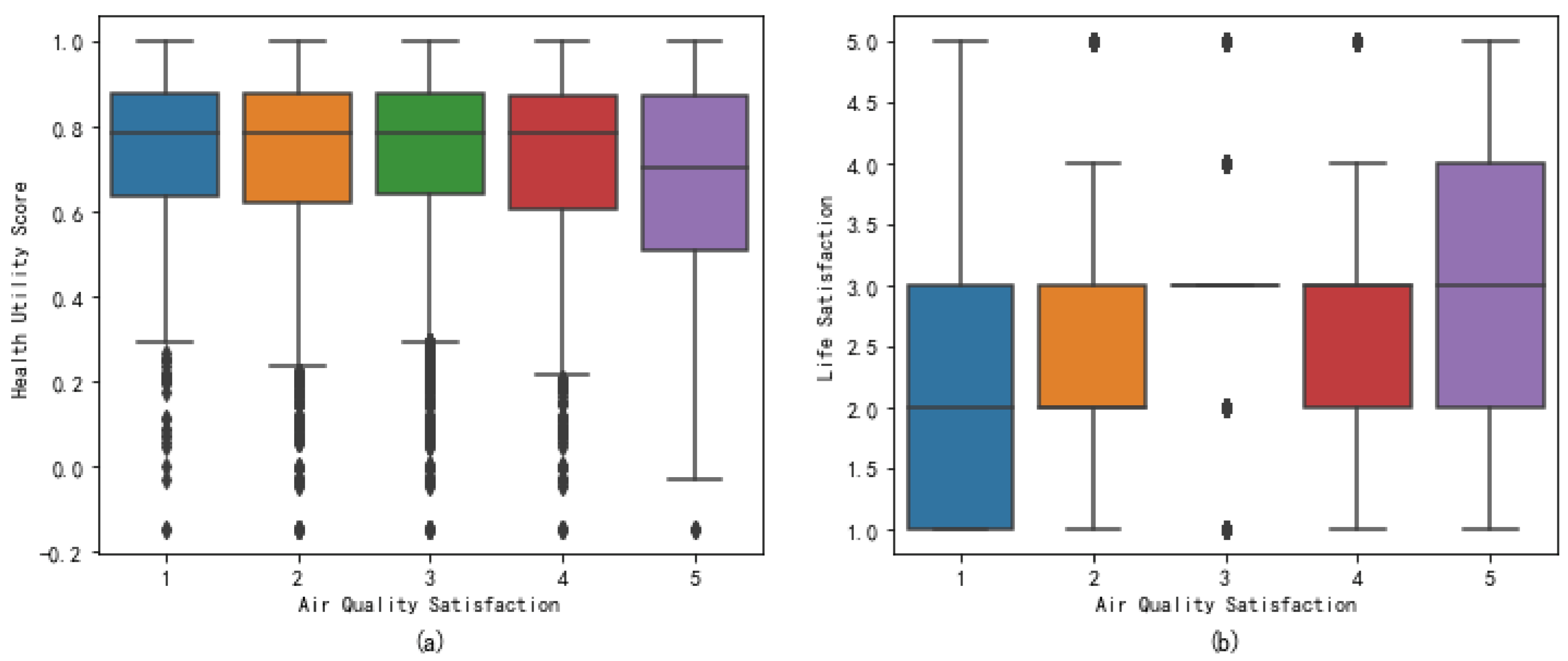
This paper took residents’ subjective evaluation of air quality satisfaction (X1) as the core variable that affects residents’ QOL in 2018. The subjective evaluation question regarding air quality was expressed as “How satisfied are you with the air quality this year (2018)?” The value for this was 1–5, where 1 = completely satisfied, 2 = very satisfied, 3 = somewhat satisfied, 4 = not very satisfied, 5 = not at all satisfied. The discrete distribution of air quality satisfaction, QOL health utility EQ-5D and experienced utility for life satisfaction is shown in Figure 1. For samples with a standard normal distribution, only a few values were outliers. There are only six outliers in the right figure of Figure 1, indicating that the distribution has almost no tail and a large degree of freedom. The outliers in the left figure are concentrated on the side with the lower health utility value, indicating that the distribution of air quality satisfaction and the health utility value shows a slight leftward skew.

2.3.3. Control Variables

In order to eliminate the estimation error caused by missing variables as much as possible, other individual characteristics that may affect the health utility of residents’ QOL were introduced as control variables—sex, residence areas, education background, marital status, smoking status, drinking, sleeping status and individual yearly income—to control the impact of personal characteristics and lifestyle on residents’ QOL regarding the health utility. When taking the QOL regarding the experienced utility for life satisfaction as the explanatory variable for logical progression, in addition to the above control variables, three satisfaction indicators of health satisfaction, marital satisfaction and children satisfaction were added as supplementary control variables to control the impact of residents’ subjective evaluation indicators on residents’ life satisfaction. The value was 1–5, where 1 = completely satisfied, 2 = very satisfied, 3 = somewhat satisfied, 4 = not very satisfied, 5 = Not at all satisfied. The specific assignment of variables is shown in

Table 2. Dummy variables assignment.

Variables	Assignment and Meaning
Sex (X2)	Male = 0; Female = 1
Residence Areas (X4)	Other = 0; Village = 1
Education Background (X5)	Primary school or below = 0; Secondary school or above = 1
Marital Status (X6)	Widowed/Divorced/Separated/Unmarried = 0; Married = 1
Smoking Status (X7)	Non-smokers = 0; Smoking history = 1
Drinking (X8)	No drinking = 0; Drinking = 1
Sleeping Status (h) (X9)	Abnormal (<5 h or >9 h) = 0; Normal ([5 h,9 h]) = 1
Health Satisfaction (X11)	1 = Completely satisfied, 2 = Very satisfied, 3 = Somewhat satisfied, 4 = Not very satisfied, 5 = Not at all satisfied
Marital Satisfaction (X12)	1 = Completely satisfied, 2 = Very satisfied, 3 = Somewhat satisfied, 4 = Not very satisfied, 5 = Not at all satisfied
Children Satisfaction (X13)	1 = Completely satisfied, 2 = Very satisfied, 3 = Somewhat satisfied, 4 = Not very satisfied, 5 = Not at all satisfied

.

For education background, the score spanned from 1 to 11, where 1 = no formal education (illiterate), 2 = did not finish primary school, 3 = sishu/home school, 4 = elementary school, 5 = middle school, 6 = high school, 7 = vocational school, 8 = two-/three-year college/associate degree, 9 = four-year college/Bachelor’s degree, 10 = Master’s degree, 11 = doctoral degree/Ph.D. In Table 2, education background (X5) ranges from 0 to 1. As a control variable, education background did not significantly affect the size of the regression coefficient of the explained variables in the model, which made the problem description more concise. Therefore, it was used as a dummy variable reflecting education level for modeling.

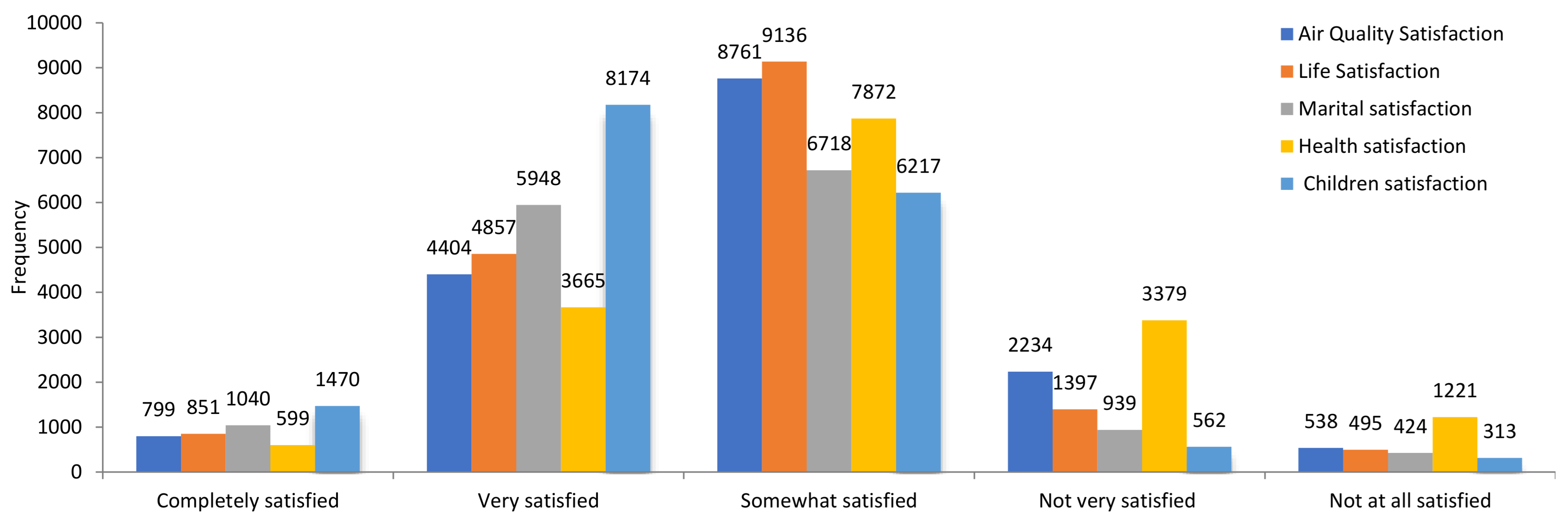
The frequency chart of the subjective perception of middle-aged and elderly Chinese residents is shown in Figure 2, from which it can be seen that the subjective perception of residents is generally normally distributed.

Considering the actual significance of the data, the variables age (years) and yearly individual income used the original data to participate in the regression.

3. Models and Methods

3.1. T Test and Pearson Correlation Analysis

In order to ensure the accuracy of the sample and the correctness of the model, the t-test and the Pearson correlation coefficient test were carried out on the influencing factors of QOL. The factors that were significant at the significance level of 5% in both tests were included in the regression model.

3.2. Multicollinearity Test

In order to avoid the possible multiple collinearities between explanatory variables, this paper used the Variance Inflation Factor (VIF) method to test the possible collinearity between variables before establishing the model. This method mainly judges whether there is multicollinearity between variables through the size of variance inflation factor. We took the explanatory variable Xi (i = 1, 2, …, 13) as the dependent variable, and the other explanatory variables other than Xi as the independent variables and established a linear regression model to obtain the decisive factor. The calculation formula of variance inflation factor is as follows:

$$\mathrm{VIF}=\frac{1}{1-{\mathrm{R}}_{\mathrm{i}}^2}$$

(2)

where R² is the determination coefficient of regression to other explanatory variables when the explanatory variable Xi (i = 1, 2, …, 13) is the dependent variable.

The multicollinearity test showed that the value of variance expansion factor VIF between explanatory variables was between 1.02 and 1.45, indicating that there was no multicollinearity between explanatory variables.

3.3. Multivariate Linear Regression Model

In order to test the impact of air quality satisfaction on the EQ-5D score of the health utility of residents’ QOL, based on the existing research experienced and available data, a multi factor linear regression model was set:

$${\mathrm{QOL}}_{\mathrm{i}}=u_i+\alpha {\mathrm{AQS}}_{\mathrm{i}}+\beta Contro{l}_{\mathrm{i}}+{\epsilon }_{\mathrm{i}}$$

(3)

Here, the core explanatory variable is air quality satisfaction (AQS), and the control variables include variables related to QOL: age, residence areas, sex, marital status, drinking, smoking status, sleeping status, education background and individual yearly income. $u_i$ represents a fixed effect, ${\epsilon }_{\mathrm{i}}$ represents a random disturbance item, and i represents the individual respondent.

3.4. Binomial Logistic Regression Model

The binomial logistic regression model was established to carry out comprehensive evaluation among various influencing factors, to analyze the influencing factors of life satisfaction. This method can better solve the problem of interdependence among influencing factors.

The binomial logistic regression model is as follows:

$$\left\{\begin{array}{l}{\mathrm{Z}}_{\mathrm{i}}=Ln\frac{{\mathrm{P}}_{\mathrm{i}}}{1-{\mathrm{P}}_{\mathrm{i}}}=u_{\mathrm{i}}+\alpha {\mathrm{AQS}}_{\mathrm{i}}+\beta Contro{l}_i+{\epsilon }_{\mathrm{i}}\\ g(z)=\frac{1}{1+e^{-Z}}\\ P(Y_2=1|w,x)=g(z)\\ P(Y_2=0|w,x)=1-g(z)\\ \mathrm{odds}=\frac{\mathrm{P}}{1-\mathrm{P}}\end{array}\right.$$

(4)

where Pi is the probability of life satisfaction, the probability of life dissatisfaction is (1-pi), Pi ∈ (0,1), and odds is the ratio of the probability of life satisfaction to the probability of life dissatisfaction. Zi represents the explained variable residents’ life satisfaction, and the core explanatory variable is air quality satisfaction. The control variables include variables related to QOL: health satisfaction, marriage satisfaction, children satisfaction, age, residence areas, sex, marital status, drinking, smoking status, sleeping status, education background and individual yearly income. $u_i$ is a fixed effect, ${\epsilon }_{\mathrm{i}}$ is a random disturbance item, and i is the individual respondent.

As the subjective perception factors entering the logistic regression equation were air quality satisfaction, health satisfaction, marriage satisfaction and child satisfaction, the assignment of the classification level was arranged from small to large according to its logical meaning, which is opposite to the logical order of the dependent variable (life satisfaction) (0 = dissatisfaction, 1 = satisfaction). Therefore, when the estimated coefficient value of these subjective perception variables was negative in the regression model, it indicated that the smaller the value of this variable, the greater the possibility of life satisfaction. Among other control variables, education level, individual yearly income and sleeping status had the same logical order with life satisfaction, indicating that the greater the value of these variables, the greater the probability of life satisfaction.

4. Analysis of Influencing Factors of QOL

4.1. Single Factor Analysis of QOL

The results of the univariate analysis of the QOL are shown in

Table 3. T-test and Pearson’s correlation of influencing factors.

Variables	Explained Variable: EQ-5D Score		Explained Variable: Life Satisfaction
Explanatory Variables	t Test t(p)	Pearson’s Correlation r(p)	t Test t(p)	Pearson’s Correlation r(p)
Air Quality Satisfaction (X1)	−315.101 *** (0.0)	−0.065 *** (3.99 × 10−17)	−284.030 *** (0.0)	−0.155 *** (1.87 × 10−90)
Sex (X2)	52.367 *** (0.0)	−0.186 *** (1.37 × 10−130)	80.315 *** (0.0)	−0.065 *** (4.57 × 10−17)
Age (years) (X3)	−835.15 *** (0.0)	−0.188 *** (1.35 × 10−133)	−832.93 *** (0.0)	0.04 *** (2.34 × 10−7)
Residence Areas (X4)	−0.275 (0.784)	−0.104 *** (3.76 × 10−41)	34.556 *** (1.041 × 10−256)	−0.053 *** (7.10 × 10−12)
Education Background (X5)	94.647 *** (0.0)	0.234 *** (7.76 × 10−207)	120.050 *** (0.0)	0.058 *** (6.45 × 10−14)
Marital Status (X6)	−39.619 *** (0.0)	−0.128 *** (4.21 × 10−62)	5.625 *** (1.87 × 10−8)	0.058 *** (4.67 × 10−14)
Smoking Status (X7)	305.164 *** (0.0)	0.022 ** (0.004)	295.453 *** (0.0)	−0.005 (0.523)
Drinking (X8)	96.699 *** (0.0)	0.170 *** (3.09 × 10−108)	121.996 *** (0.0)	0.051 *** (2.86 × 10−11)
Sleeping Status (X9)	−6.678 *** (2.46 × 10−11)	0.245 *** (1.02 × 10−226)	29.489 *** (1.63 × 10−188)	0.107 *** (1.45 × 10−43)
Individual yearly Income (X10)	−68.389 *** (0.0)	0.177 *** (3.16 × 10−118)	−68.388 *** (0.0)	0.078 *** (1.01 × 10−23)
Health Satisfaction (X11)			−287.616 *** (0.0)	−0.323 *** (0.0)
Marital Satisfaction (X12)			−199.239 *** (0.0)	−0.201 *** (2.09 × 10−151)
Children Satisfaction (X13)			−228.362 *** (0.0)	−0.199 *** (2.52 × 10−148)

* p < 0.05, ** p < 0.01, *** p < 0.001. Notes: p values are in parentheses. To save space, only parameters of key interest are presented, but results of the full models are available upon request.

. The results of correlation analysis show that air quality satisfaction, sex, age (years), education background, marital status, drinking, sleeping status and individual year income were the significant influencing factors of health utility value (EQ-5D) (p < 0.05). There was no difference between residence and health utility value in the t-test (p > 0.05), and the residence area factor was not included in the linear regression model.

The fourth and fifth columns of Table 3 show the results of the t-test and Pearson correlation analysis of life satisfaction with the 13 influencing factors. The results of the analysis showed that air quality satisfaction was correlated with life satisfaction at a significance level of 0.1%. Sex, age (years), residence areas, educational background, marital status, drinking, sleeping status, individual yearly income, health satisfaction, marital satisfaction and children satisfaction were influential factors in experiencing utility value for life satisfaction (p < 0.05). Smoking status was not significant in Pearson’s correlation test (p > 0.05), and smoking status was not included in the logistic regression model. This is inconsistent with the research results of Wang, H. et al. [13].

4.2. Multi-Factor Linear Regression Analysis of Factors Influencing Health Utility

The linear regression model was constructed by taking the significant variables of univariate analysis, air quality satisfaction, sex, age (years), education background, marital status, smoking status, drinking, sleeping status and individual yearly income as explanatory variables and the health utility value of QOL (EQ-5D) as the explained variable to test the effect of air quality satisfaction on the health utility of residents’ QOL, and the regression results are shown in

Table 4. Multiple linear regression analysis of factors influencing health utility values (n = 16,736).

Variables	Health Utility EQ-5D Score
Explanatory Variables	Model 1	Model 2	Model 3
Air Quality Satisfaction (X1)	−0.018 *** (0.002)	−0.0235 *** (0.002)	−0.0235 *** (0.002)
Sex (X2)		−0.0464 *** (0.004)	−0.0472 *** (0.004)
Age (years) (X3)		−0.0032 *** (0.000)	−0.0032 *** (0.000)
Education Background (X5)		0.0403 *** (0.004)	0.0402 *** (0.004)
Marital Status (X6)		0.0262 *** (0.006)	0.0260 *** (0.006)
Smoking Status (X7)			−0.0139 (0.008)
Drinking (X8)		0.0330 *** (0.004)	0.0332 *** (0.004)
Sleeping Status (X9)		0.0978 *** (0.004)	0.0977 *** (0.004)
Individual Income (X10)		9.876 × 10−7 *** (9.85 × 10−8)	9.94 × 10−7 *** (9.88 × 10−8)
Intercept	0.7919 *** (0.006)	0.8932 *** (0.017)	0.8944 *** (0.017)
Adj.R2	0.004	0.145	0.145
AIC	−2321	−4862	−4863
BIC	−2305	−4793	−4786

* p < 0.05, ** p < 0.01 and *** p < 0.001. Notes: Standard errors are in parentheses. To save space, only parameters of key interest are presented, but results of the full models are available upon request.

, where Model 1 is the estimation result without introducing control variables, while Model 2 and Model 3 are the estimation results after introducing control variables and correcting for heteroskedasticity.

The multi-factor linear regression model shows the significant effect of air quality satisfaction on the health utility score of residents’ QOL at the significance level of 0.001. From Model 2, on average, for each increase in air quality satisfaction level (the larger the level, the lower the air quality satisfaction), the health utility value of residents’ QOL decreases by 2.35 percentage points, when all other indicators are equal. This indicates that poorer air quality satisfaction reduces the level of health utility of residents’ QOL, and that there is a significant positive relationship between air quality satisfaction and residents’ QOL.

The regression results of other explanatory variables also provide some enlightenment. The regression coefficient of sex is significantly negative in the estimation, indicating that the QOL health utility value of female respondents is significantly lower than that of males, and the fluctuation of QOL health utility scores is somewhat greater than that of males, which may be due to the fact that most Chinese women bear the dual pressures of work and family life, and lack the ways and environment to relax. Secondly, there is a significant negative correlation between age and the health utility value of QOL, which decreases with age. The estimated value of the regression coefficient of education level is significantly positive, indicating that education can improve the ability, cognitive level and psychological resilience of residents in China, and bring about the improvement of material living standards, thus indirectly improving the QOL. The marriage factor is significant at the level of 0.001, indicating that there are significant differences in the QOL between different marital status groups. From the marital status variables, it is shown that the QOL health utility of married groups is higher, while the health utility of divorced, widowed or single groups is lower, which may be because married people obtain more utility in the form of family support. The estimated linear regression coefficient of alcohol consumption is significantly positive—a possible reason for this is that in contrast with smoking (not significant) addiction, most middle-aged and elderly people tend to drink alcohol in moderation, and only on important festivals or occasions, and that a small amount of alcohol is beneficial to their health to some extent. At the same time, the improvement of national health awareness, the increase in healthy life publicity, the diversification of publicity forms and the development of the Internet have all made middle-aged and elderly people pay more attention to the healthy lifestyle of avoiding smoking and drinking. The effect of sleep status on the health effect of the QOL is significantly positive, indicating that residents with good sleep quality are healthier than those with abnormal sleep conditions. The estimated coefficient of personal annual income is significant in the regression, but the regression coefficient is very small. In general, the higher the income of residents, the more and better medical care and services they can access, and the better their QOL. However, due to the possible “happiness paradox” phenomenon, an increase in an individual’s annual income does not necessarily lead to an improvement in the QOL.

According to the absolute value of the estimated value of the regression coefficient, the magnitude of the effect of each of the variables entering the regression equation on the utility value of QOL can be ranked, in descending order, as sleep status, gender, education, alcohol consumption, marital status, air quality satisfaction, age and annual personal income.

4.3. Multi-Factor Logistic Regression Analysis of Influencing Factors of Experienced Utility

The significant influencing factors which were significant in the univariate analysis include air quality satisfaction, sex, age (years), residence areas, education background, marital status, drinking, sleeping status, individual yearly income, health satisfaction, marital satisfaction and child satisfaction. Life satisfaction was taken as the dependent variable to construct a multi-factor binary logistic regression model.

The regression results are shown in

Table 5. Binomial logistic regression analysis of factors influencing experienced utility (n = 16736).

	Life Satisfaction
Explanatory Variables	Model 3	Model 4	Model4 Exp (β)	Model 5	Model 6
Air Quality Satisfaction (X1)	0.6568 *** (0.0084)	−0.3250 *** (0.0343)	0.7225	−0.3258 *** (0.0343)	−0.3259 *** (0.0343)
Sex (X2)				0.0485 (0.0593)	0.0585 (0.0644)
Age (years) (X3)		0.0301 *** (0.0032)	1.03055	0.0304 *** (0.0032)	0.0305 *** (0.0032)
Residence Areas (X4)		−0.1635 * (0.0740)	0.8492	−0.1563 * (0.0745)	−0.1562 * (0.0745)
Education Background (X5)		0.1958 ** (0.0651)	1.2163	0.2050 ** (0.0660)	0.2043 ** (0.0661)
Marital Status (X6)		−0.8260 *** (0.1159)	0.4378	−0.8311 *** (0.1162)	−0.8317 *** (0.1162)
Drinking (X8)					0.0267 (0.0667)
Sleeping Status (X9)		0.3691 *** (0.0604)	1.4464	0.3729 *** (0.0605)	0.3729 *** (0.0605)
Individual yearly Income (X10)		0.0000 *** (0.0000)	1.0	0.0000 *** (0.0000)	0.0000 *** (0.0000)
Health Satisfaction (X11)		−0.9954 *** (0.0330)	0.3696	−0.9972 *** (0.0331)	−0.9962 *** (0.0332)
Marital Satisfaction (X12)		−0.4975 *** (0.0328)	0.6080	−0.5019 *** (0.0333)	−0.5021 *** (0.0333)
Children Satisfaction (X13)		−0.3426 *** (0.0326)	0.7099	−0.3392 *** (0.0329)	−0.3392 *** (0.0329)
Intercept		7.5124 *** (0.3326)		7.4694 *** (0.3366)	7.4480 *** (0.3407)
Pseudo R^2	−0.131	0.226		0.226	0.226
AIC	13,357.42	9168.41		9169.75	9171.59
BIC	13,365.14	9253.39		9262.93	9272.01

* p < 0.05, ** p < 0.01, *** p < 0.001. Notes: Standard errors are in parentheses. To save space, only parameters of key interest are presented, but results of the full models are available upon request.

, where Model 3 is the estimation result without introducing control variables, and Model 4, Model 5 and Model 6 are the estimation results after introducing the control variables and gradually removing insignificant factors using the backward elimination method. Exp(β) represents the estimated value of the change multiple of the ratio of the probability of life satisfaction to the probability of life dissatisfaction (odds) caused by the increase in one unit of the i-th explanatory variable and reflects the magnitude of the effect of each explanatory variable on the explained variable. The value of Exp(β) indicates that the lower the classification level of the independent variable, the greater the probability that the resident is satisfied with his or her life.

4.3.1. Results

At the 0.1% significance level, the estimated value of the regression coefficient of air quality satisfaction is negative—that is, it is significant. In Model 4, its Exp(β) value is 0.7225—that is, when all other indicators are equal, the air quality satisfaction increases by one level (the higher the level, the worse the air quality satisfaction), and the ratio of the probability of dissatisfaction life to the probability of life satisfaction (odds) is 0.7225 times the original value. This indicates that poorer air quality satisfaction can reduce life satisfaction, which means that there is a significant positive correlation between air quality satisfaction and the experienced utility level of residents’ QOL. This is consistent with the research result that the objective measurement of air quality will indirectly affect residents’ life satisfaction [3]. The estimated value of the logistic regression coefficient of the control variable age is significantly positive. According to the actual situation in China, it is stipulated that 45–59 years old represents early old age, 60–79 years old represents old age, and 80 years old or older is the longevity period. (https://baike.sogou.com/, accessed on 7 October 2021) The respondents’ life satisfaction is low in early old age, which is consistent with the fact that they are at a specific age and need to face the greatest pressures and responsibilities in their life, such as heavy work, purchasing a house and raising children.

Secondly, the regression coefficient of residence is significantly negative in the estimation (p < 0.05), indicating that the possibility of life satisfaction of rural respondents is greater than that of non-rural respondents. The higher the education level and the better the sleep status, the greater the probability of life satisfaction of middle-aged and elderly residents. The logistic regression coefficients of gender, drinking and smoking are not significant in this estimation.

The regression coefficients of health satisfaction, marital satisfaction and child satisfaction were significantly negative (p < 0.001), and the Exp(β) values were 0.3696, 0.6080 and 0.7099, respectively, indicating that the higher the classification level of subjective perception factors, the more the marginal effect of life satisfaction of the residents showed a considerable positive effect. That is, health satisfaction, marital satisfaction and children satisfaction show significant positive correlations with life satisfaction.

According to the magnitude of Exp(β) values in Model 4, the magnitude of the effect of each variable on life satisfaction that finally entered the logistic regression equation can be ranked, in descending order, as sleeping status, education background, age (years), individual yearly income, areas. air quality satisfaction, children satisfaction, marital satisfaction, marital status, and health satisfaction.

If the probability of life satisfaction is set to p (the probability of life dissatisfaction is (1-p), p ∈ (0,1)), and the logit transformation of p is the dependent variable, a logistic regression model is constructed according to the logistic regression formula using direct logistic regression coefficients:

$$\begin{array}{ll}\log \left(\mathrm{p}\right)=& 7.5124-0.3250\times {\mathrm{X}}_1+0.0301\times {\mathrm{X}}_3-0.1635\times {\mathrm{X}}_4+0.1958\times {\mathrm{X}}_5-0.8260\times {\mathrm{X}}_6\\ & +0.3691\times {\mathrm{X}}_9-0.9954\times {\mathrm{X}}_{11}-0.4975\times {\mathrm{X}}_{12}-0.3426\times {\mathrm{X}}_{13}\end{array}$$

(5)

4.3.2. Model Evaluation

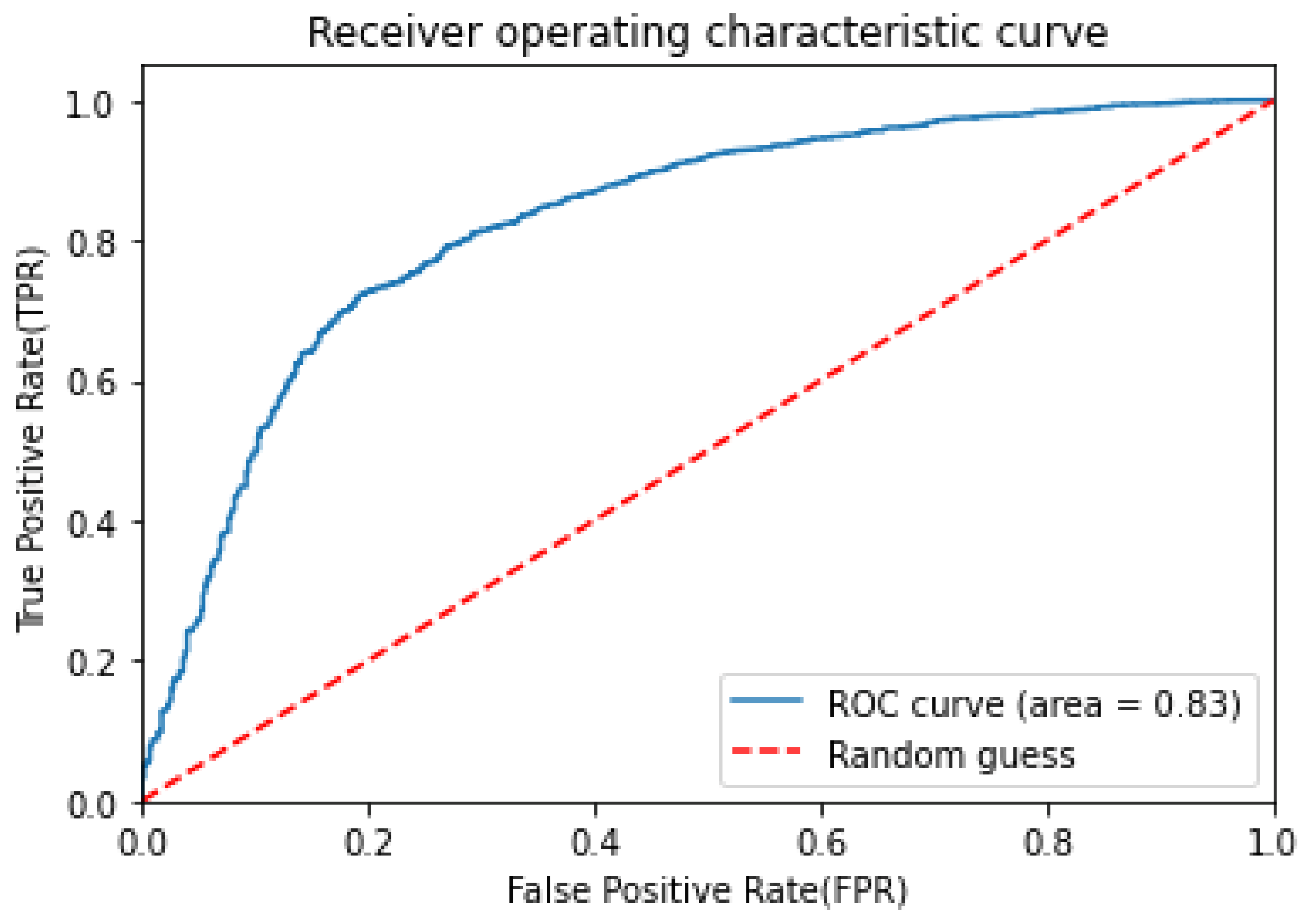
To evaluate the accuracy of the model, all 16,736 samples were divided into a training set and a test set in logistic regression—11,715 samples in the training set and 5021 samples in the test set were evaluated using logistic regression analysis. The overall prediction fit accuracy of the regression equation classification prediction was 0.89 (classification truncation was taken as 0.50), and 14,895 samples out of 16,736 samples were correctly classified. The accuracy of life satisfaction classification was 0.89.

From the Receiver Operating Characteristic curve (ROC) is shown in Figure 3, it can be seen that the Area Under Curve (AUC) value of the optimal critical point of the area covered by the ROC curve is 0.83, because a larger value represents a better effect of logistic regression analysis, which means the model has a good prediction effect. The recall rate of the number of truly positive cases predicted is 0.99, and the recall rate of the number of truly negative cases predicted is 0.17. The overall discriminant accuracy of the estimated samples is 88.99%—that is, the overall accuracy of the model prediction is good.

4.4. Robustness Analysis

The regression results remain robust in the following robustness tests:

(1).

The replacement of the dependent variable. The “experienced utility” life satisfaction of QOL is used to replace the EQ-5D score of health utility for regression analysis. After the replacement, the explanatory variable air quality satisfaction is still positive at the significant level of 1%. The better the air quality satisfaction, the greater the possibility of life satisfaction, which is consistent with the results of the article findings [1,2]. This shows that the subjective evaluation of air quality is indeed positively correlated with residents’ QOL, and the improvement of air quality helps to improve residents’ QOL. Additionally, other explanatory variables and their related variables are significantly correlated with QOL.

(2).

Add control variables. Considering that life satisfaction indicators of QOL experienced utility are subjective perception data, which are influenced by residents’ cognitive level and other aspects, variables such as health satisfaction, marital satisfaction and child satisfaction were added as control variables. After adding the control variables, the regression also shows that the estimated coefficients of air quality satisfaction are significantly positive, and the estimated values of the regression coefficients of the subjective perception category control variables are all significant, and the conclusion maintains that the higher the air quality satisfaction, the better the QOL of the residents.

(3).

The replacement model test. A multi-factor linear regression model was established for the analysis of the correlation between air quality satisfaction and health utility values. The multi-factor logistic regression model was used to test the relationship between air quality satisfaction and life satisfaction, and the positive effect of air quality satisfaction on residents’ life satisfaction passed the significance test at the 1% significance level, which was consistent with the statistical results of the multiple linear regression model. The worse the air quality satisfaction, the lower the residents’ life satisfaction and the worse the QOL, and the regression results remain robust.

5. Conclusions and Discussion

This paper uses the 2018 China Health and Retirement Longitudinal Study (CHARLS) database, using multi-factor linear regression and binary logistic regression methods to examine the relationship between subjective air quality assessment and the QOL of Chinese middle-aged and elderly residents. The two models produced consistent results regarding a significant positive relationship between air quality satisfaction and QOL. This is consistent with the finding that there is a significant positive correlation between air quality (outdoor air-PM₁₀) and QOL [2]. Exploring the relationship between subjective evaluation of air quality and the QOL of residents has important practical significance. From the government’s point of view, the local air quality reflects the government’s environmental governance performance to a certain extent. With regard to the subjective feelings of residents, the air quality of the place of residence will directly affect the quality of their daily life, thereby affecting their subjective evaluation of the air quality status.

This study analyzed the impact of air quality satisfaction on the QOL from the two dimensions of the health utility and experienced utility of the QOL and concludes that there is a significant positive correlation between air quality satisfaction and QOL. The impact of gender and income on the QOL of middle-aged and elderly residents is statistically significant (p < 0.05), but this impact is indirect and limited. The influence of lifestyle factors on the QOL cannot be ignored. The significance of the impact of the interviewee’s residence and smoking status on the QOL and health utility needs to be further verified.

In this study, we used the CHARLS 2018 database to analyze the impact of the subjective assessment of air quality on the QOL. We put forward the “two-dimensional” research perspective of QOL, which divides the QOL into two different dimensions: the health utility of the QOL and the experienced utility of the QOL and perform beneficial exploration and research to investigate the correlation between subjective evaluation of air quality and QOL. One of the main shortcomings of this study is that the subjective assessment of air quality is not comprehensive enough, and there is no specific index assessment involving air quality. Despite this shortcoming, this research better reflects the problems of environment-related QOL, and draws several conclusions:

Firstly, China should reform the current performance assessment system and increase the weight of environmental assessment indicators. The government should thus carry out the air quality satisfaction assessment of urban and rural residents based on questionnaire surveys, and take the public satisfaction assessment as one of its main data sources in the assessment system of atmospheric environment governance, in order to improve the assessment method of comprehensive improvement of atmospheric environment, and thus to improve the living standards of residents by enabling the local government to provide more high-quality air public goods.

Secondly, since the improvement of air quality can significantly enhance residents’ air quality and life satisfaction, the government needs to improve not only the local air quality, but also residents’ subjective perception of air quality. The government should establish a government-led model of air governance with the participation of stakeholders, encourage and guide the public to participate in air quality protection actions, and actively promote the participation of individuals and civil environmental groups in air governance actions.

Thirdly, by establishing an atmospheric environmental education system to increase the publicity of atmospheric environmental knowledge improve the public’s attention to air quality, the government will increase the public’s environmental awareness and enrich environmental knowledge, as well as strengthening the publicity regarding the significance of individual environmental behaviors. This will provide residents with the belief that personal behavior can have a profound impact on atmospheric environmental protection.

Due to the limitations of the complexity of the factors affecting the QOL and the availability of data, this article still has the following drawbacks: on the one hand, this article mainly considers the influence of the subjective assessment of the overall air quality of residents on the QOL and does not involve the evaluation of specific indicators of air quality. On the other hand, this article lacks analysis of the correlation between other evaluation indicators and residents’ QOL, such as the quality of the ecological environment, drinking water, the green environment, the pollution of rivers and lakes, the degree of soil pollution, and noise pollution. The interaction between the subjective evaluation of ecological environment quality and the QOL also needs to be studied in the future.