Article

Seasonal Variations in the Daily Mortality Associated with Exposure to Particles, Nitrogen Dioxide, and Ozone in Stockholm, Sweden, from 2000 to 2016

1
Institute of Family Medicine and Public Health, Faculty of Medicine, University of Tartu, Ravila 19, 50411 Tartu, Estonia
2
Atmospheric Science Unit, Department of Environmental Science, Stockholm University, 11418 Stockholm, Sweden
3
Environment and Health Administration, SLB-analys, Box 8136, 104 20 Stockholm, Sweden
4
Section of Sustainable Health, Department of Public Health and Clinical Medicine, Faculty of Medicine, Umeå University, 901 87 Umeå, Sweden
*
Author to whom correspondence should be addressed.
Atmosphere 2021, 12(11), 1481; https://doi.org/10.3390/atmos12111481
Submission received: 14 October 2021 / Revised: 3 November 2021 / Accepted: 5 November 2021 / Published: 9 November 2021
(This article belongs to the Special Issue Health Effects of Urban Atmospheric Aerosols)

Abstract

:
Urban air pollutant emissions and concentrations vary throughout the year due to various factors, e.g., meteorological conditions and human activities. In this study, seasonal variations in daily mortality associated with increases in the concentrations of PM10 (particulate matter), PM2.5–10 (coarse particles), BC (black carbon), NO2 (nitrogen dioxide), and O3 (ozone) were calculated for Stockholm during the period from 2000 to 2016. The excess risks in daily mortality are presented in single and multi-pollutant models during the whole year and divided into four different seasons, i.e., winter (December–February), spring (March–May), summer (June–August), and autumn (September–November). The excess risks in the single-pollutant models associated with an interquartile range (IQR) increase for a lag 02 during the whole year were 0.8% (95% CI: 0.1–1.4) for PM10, 1.1% (95% CI: 0.4–1.8) for PM2.5–10, 0.5% (95% CI: −0.5–1.5) for BC, −1.5% (95% CI: −0.5–−2.5) for NO2, and 1.9% (95% CI: 1.0–2.9) for O3. When divided into different seasons, the excess risks for PM10 and PM2.5–10 showed a clear pattern, with the strongest associations during spring and autumn, but with weaker associations during summer and winter, indicating increased risks associated with road dust particles during these seasons. For BC, which represents combustion-generated particles, the pattern was not very clear, but the strongest positive excess risks were found during autumn. The excess risks for NO2 were negative during all seasons, and in several cases even statistically significantly negative, indicating that NO2 in itself was not harmful at the concentrations prevailing during the measurement period (mean values < 20 µg m−3). For O3, the excess risks were statistically significantly positive during “all year” in both the single and the multi-pollutant models. The excess risks for O3 in the single-pollutant models were also statistically significantly positive during all seasons.

1. Introduction

While air pollutant emissions occur throughout the whole year, differences in meteorological conditions and human activities cause large seasonal variations in most pollutants. Kukkonen et al. (2000) [1] showed that meteorological variables in northern Europe vary widely with the seasons and, consequently, those variations are reflected in urban air quality. Apart from anthropogenic and natural emissions, among the main factors influencing seasonal variations in air quality are occurrence of temperature inversions, wind speed, precipitation, and solar radiation [2]. Particularly in the Nordic countries, where studded winter tires are used, suspension of coarse particles from road surfaces is highly dependent on surface moisture, which shows very large variations during the year, and with a major impact on the seasonal variations in the concentrations of both PM10 and PM2.5 [3].
The seasonal variations in air quality give rise to differences in health effects. In a study from the Netherlands, the associations between daily mortality and short-term variations in a number of air pollutants were analyzed during the period from 1986 to 1994, and the results were, among other things, divided into summer and winter seasons [4]. They found significantly (95% CI) increased relative risks for all pollutants (PM10, BS (black smoke), O3, SO2, NO2, CO, SO4−2, and NO3) during both summer and winter, except for O3 and SO4−2 during the winter. Moreover, the relative risks for total mortality associated with exposure to these air pollutants were in all cases larger during the summer compared to the winter [4].
Seasonal variations regarding short-term health effects associated with exposure to PM10 have been analyzed in a number of studies. When increased mortality associated with an increase in PM10 was analyzed in 100 cities in the U.S. in the period from 1987 to 2000, a significant association was found for the summer period, but no significant associations were found for the other three seasons. The seasonal pattern was also more pronounced in the northeast region of the U.S., while there were relatively small seasonal variations in the southern regions [5]. In Flanders, Belgium, where daily mortality associated with PM10 was calculated during the period from 1997 to 2003, and where temperature and seasons were included as potential effect modifiers, the strongest associations were also found during the summer [6]. Similarly, a significate effect of PM10 on mortality increase during the summer was found in Tallinn, Estonia, during the period from 2004 to 2011 [7]; however, during the winter, a significant decrease in mortality associated with an increase in PM10 appeared. In a study from China, where the association between daily mortality and an increase in PM10 was analyzed in 17 Chinese cities during different seasons, significant associations were found for summer and winter, but not for spring and autumn [8]. In another study from Wuhan, China, conducted from 2001 to 2004, the strongest associations for PM10 were found during winter [9]. In a study from Korea, where the associations between PM10 concentrations and increases in mortality and hospital admissions were analyzed in Seoul from 2000 to 2006, the effects on both mortality and morbidity increased during the summer [10]. Finally, in a study from Utah, U.S., the association between daily mortality and exposure to PM10 was examined for the period 1985 to 1992. The largest contribution to excess mortality was for individuals 75+ years old dying in a hospital, and the strongest effect was shown during the spring [11].
Seasonal variations regarding short-term effects on hospitalization for cardiovascular diseases associated with PM2.5 were analyzed in New York State during the period 1991 to 2006. The strongest effects, associated with a 10 µg m−3 increase in PM2.5, were found during the winter. Temperature modified the PM2.5 effects on cardiovascular diseases, and these effects were found on low temperature days [12]. In a study in Tallinn, PM2.5 increased mortality during the summer, but no effects appeared during the winter [7].
For particles in the coarse fraction (PM2.5–10), the difference in short-term effects on daily mortality between two annual periods was analyzed in Stockholm during the period from 2000 to 2008. The associations between PM2.5–10 and daily mortality were stronger during November to May in comparison with the rest of the year, which can be explained by the high levels of road dust that occurs because of the use of studded tires in Stockholm during this time of the year [13].
The seasonal variations in short-term effects associated with NO2 were analyzed in a study from China. The daily mortality associated with NO2 in the city of Shenzhen in southeastern China during the period from 2013 to 2017 was analyzed during the cold season (November–April) and during the warm season (May–October). Significant excess risks for cardiovascular mortality associated with an increase in NO2 were found during the cold season at a 2-day lag and at a 6-day lag. However, no significant excess risks were found during the warm season [14].
The short-term health effects associated with O3 and their seasonal variations have been studied in U.S., France, and China. When the short-term mortality effects associated with O3 were analyzed in 20 communities in U.S., and where ten communities represented the northern part and ten represented the southern part, the seasonal variations in the effects estimates exhibited different results in the northern and southern parts. In the southern communities, an increase in O3 entailed increases in mortality during autumn and winter, while there were negative excess risks during spring and summer. In the northern communities, an increase in mortality was found during spring, summer and autumn, while there was a negative excess risk during the winter. In this study, latitude and seasonal average temperature were identified as effect modifiers [15]. In a study in nine French urban areas during the period from 1998 to 2006, the association between daily mortality and the daily max-8 h O3 concentrations was analyzed by season and by temperature strata. The strongest mortality effects were found during the summer and for the highest temperature strata [16]. In a study from China, the association between O3 and daily mortality was analyzed in the city of Zhengzhou during the period from 2013 to 2015. Significant excess risks associated with an increase in 10 µg m−3 24-h average O3 concentrations at a 1-day lag were found during the cold season, but not during the warm season [17].
Based on the relatively few studies referenced above, it seems like the strongest excess risks of mortality for PM10 (seven studies) and PM2.5 (only two studies) occur during the summer months. For NO2 and O3, no consistent results in terms of seasonal dependence of excess risks can be seen. However, there are very few studies: only one study for NO2, and only three studies for O3.
The purpose of the current study was to analyze the seasonal variations in the effect estimates of air pollution on mortality in Stockholm. In the earlier analyzes, only annual data were considered, but the seasonal variations were not taken into account [18]. A special focus was to analyze the causes of the negative excess risks associated with NO2, and whether the seasons and other pollutants had any effect on these associations. Seasonal differences during the year can potentially affect the results in several ways. People are more likely to stay outdoors and have windows opened during the warm seasons, which can affect the degree of exposure. Annual variations in meteorology and air pollution sources can also be of importance. In Stockholm, the chemical composition of PM10 and PM2.5–10 varies throughout the year with a significantly higher proportion of mechanically generated road dust particles during early spring [3]. Analyzing the associations between mortality and short-term exposure to the above-mentioned air pollutants during different seasons in Stockholm is, therefore, of great interest.

2. Materials and Methods

This study includes residents of Stockholm, with a population that increased from 0.8 to 0.9 million during the period from 2000 to 2016. Population data were obtained from the Swedish Central Bureau of Statistics. Cause of mortality data were obtained from the National Cause of Death Register. Natural cause of mortality is defined on the basis of the underlying cause of death, and these data include the daily number of deaths from non-external causes (ICD-10: A00–R99) occurring among the registered population.
Air pollution exposure was estimated from a central measuring station on the roof-top of a 20 m high building in the central part of Stockholm. The monitoring station was part of the city’s regulatory air pollution control network, and equipped with reference (or equivalent) instruments for regulated pollutants according to the EU air quality directive. These air pollutants included PM10 (particles with an aerodynamic diameter smaller than or equal to 10 µm), PM2.5 (particles with an aerodynamic diameter smaller than or equal to 2.5 µm), NO2 (nitrogen dioxide), and O3 (ozone) (Table 1). The O3 measurements were based on daily maximum 8-h mean values. In addition, the monitoring included measurements of unregulated black carbon (BC), and particles in the coarse fraction (PM2.5–10) estimated by subtracting PM2.5 from PM10. The period from 2000 to 2016 was divided into winter (December–February), spring (March–May), summer (June–August), and autumn (September–November) seasons.
Temperature data were collected from the urban meteorological station Observatorielunden. In this study, daily maximum temperature was used as exposure variable.
The associations between different air pollutants and daily mortality were modelled using a quasi-Poisson regression model with a logistic link function. The concept “quasi-Poisson” refers to a model that adjusts for overdispersed data, and a logistic link function defines the relationship of the dependent variables to the mean of the Poisson distributed independent variables. The modeling procedure was replicated from a previous study [18] in order to ensure comparability of the results. The model estimated the effect of an interquartile range (IQR) increase in air pollutants on daily mortality for lag 02 (average concentration during the same and the previous two days). The IQR values were calculated based on data for the whole year. Adjustments for other time-varying factors were made by assuming a linear additive effect on a logarithmic scale:
Log(Yi) = Intercept + APi + Wi + DOWi + long-term trend
where Yi represents the daily number of deaths from non-external causes, APi represents the concentration of a specific or a combination of air pollutants on day i, Wi represents variables controlling for the weather on day i using smooth spline functions for the maximum temperature and snowfall, DOWi represents the day of the week, and the long-time trend is a smooth function varying over time to capture any long-term and seasonal patterns in mortality. The effects of air pollution were estimated by using a seasonal factor resulting in individual dose-responses for each season while keeping the other variable estimates constant for the whole period. Snowfall was included since it is a risk factor for daily mortality, as described in Auger et al. (2017) [
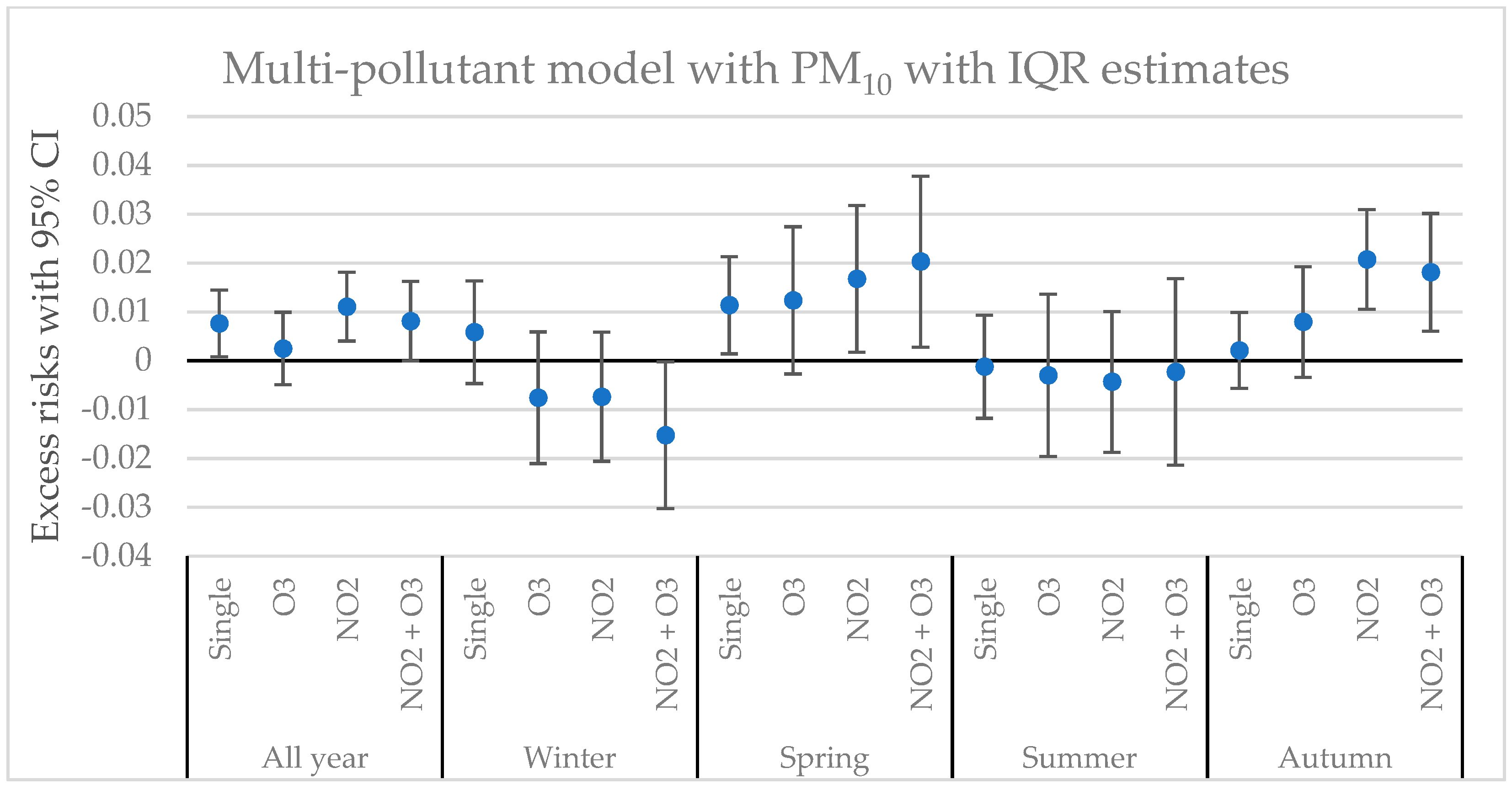
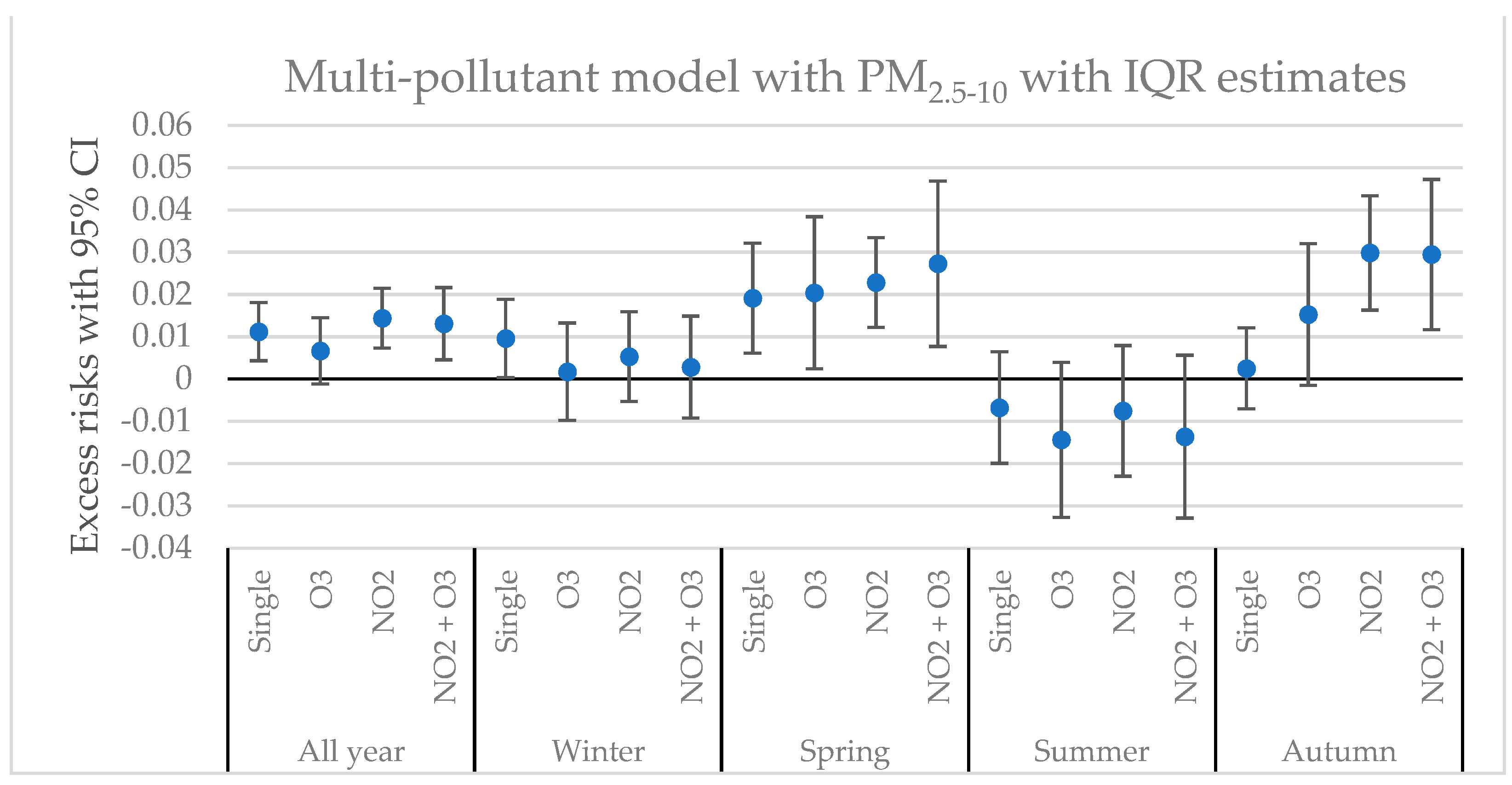
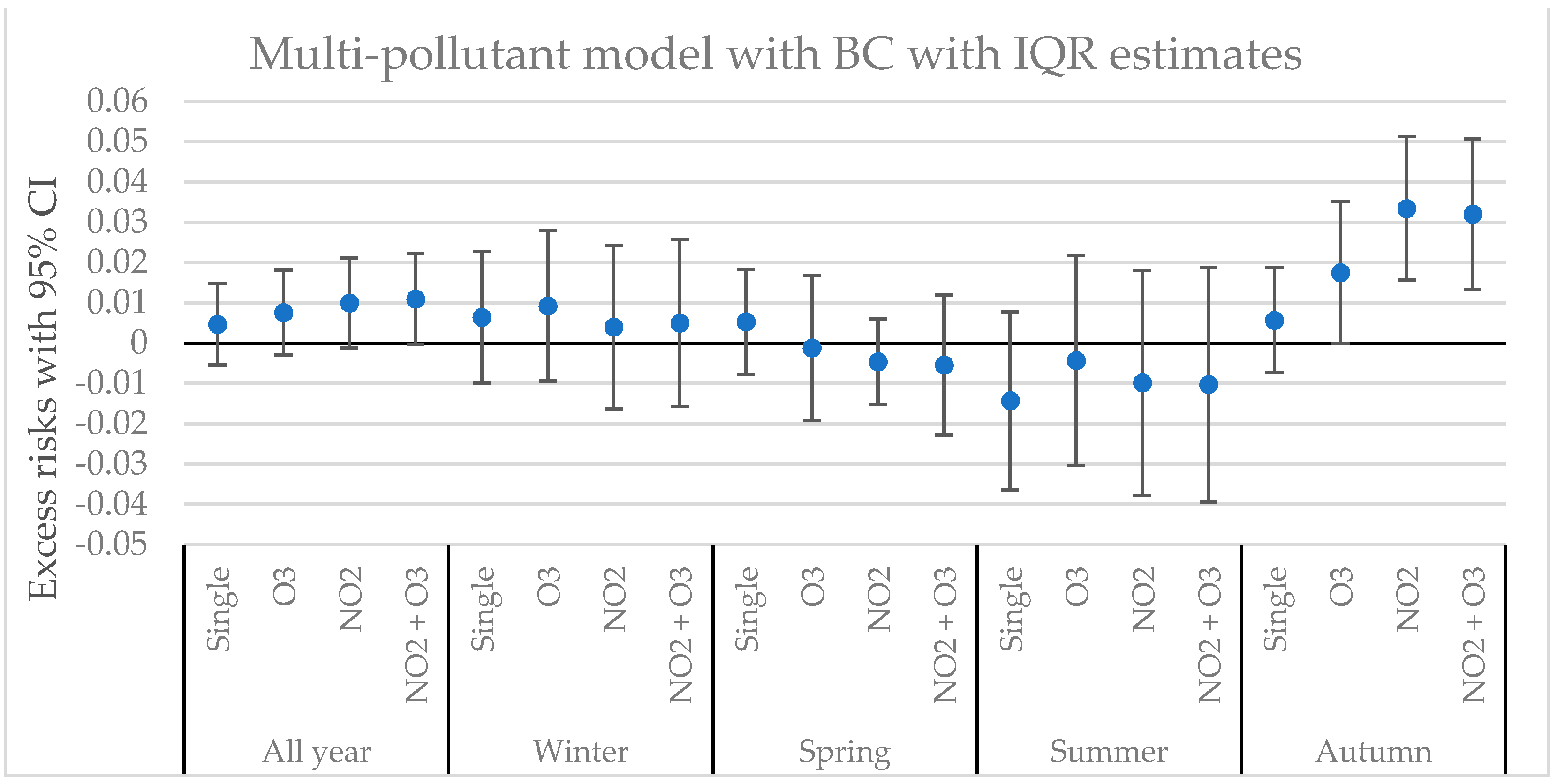
19]. The smooth function describing the long-term time trend was a penalized regression spline restricted to 5 d.f. (degrees of freedom) per year. All pollutants were modelled by assuming a linear relationship with daily mortality. Air pollutants were first modelled in single-pollutant models, and traffic-related pollutants were included in multi-pollutant models together with O3 and PM2.5–10. Temperature effects were adjusted by using two different smooth functions corresponding to the different lag-windows of 0–2 and 3–10. The model allowed for the use of 4 d.f. for each function. All analyses were conducted using R statistical software version 3.6.0 (R Foundation for Statistical Computing, Vienna, Austria).

3. Results

3.1. Descriptive Data

In Table 2, summary statistics of the daily data regarding mortality, maximum temperature, and the measured air pollutants during the period from 2000 to 2016 are presented as mean values and IQR values for the whole year, and divided into four different seasons. PM10, PM2.5–10 and O3 show the highest concentrations during spring and the lowest during autumn/winter. For NO2 and BC, the highest values are seen during winter and the lowest during summer. The seasonal variations reflect the different importance of emissions as discussed by Olstrup et al. (2019) [18].
The number of days with valid data is presented for each variable in Table A1 in Appendix A. Pearson correlation coefficients between the different air pollutants during all year and divided into different seasons are presented in Table A2, Table A3, Table A4, Table A5 and Table A6 in Appendix A.

3.2. Calculated Excess Risks

Figure 1, Figure 2, Figure 3, Figure 4, Figure 5 and Figure 6 show the calculated excess risks for daily mortality associated with an IQR increase in the measured pollutants in Stockholm during the period from 2000 to 2016. The measured air pollutants are presented in Table 2. The figures are divided into different sections where the whole year is presented furthest to the left, and then from left to right winter (December–February), spring (March–May), summer (June–August), and autumn (September–November). Figure 1 presents a single-pollutant model, and Figure 2, Figure 3, Figure 4, Figure 5 and Figure 6 present multi-pollutant models where adjustments for other pollutants have been made. The excess risks for daily mortality associated with exposure to the different air pollutants were based on lag02, which means a lagging effect of the air pollution exposure during the same and the previous two days.
The excess risks associated with exposure to PM10 and PM2.5–10 (Figure 2 and Figure 3) showed a clear pattern with the strongest associations during spring and autumn, but with weaker associations during summer and winter. For BC (Figure 4), which represents combustion-generated particles, the pattern was not very clear, but the strongest positive excess risks were found during autumn. The excess risks associated with exposure to NO2, presented in Figure 5, were significantly (95% CI) negative based on “all year”, and especially strong negative associations were shown during the autumn after adjustments for PM2.5–10 and BC. For O3 (Figure 6), the excess risks were significantly (95% CI) positive during “all year” in both the single and the multi-pollutant models. The single-pollutant models were also significantly positive during all seasons, and the highest excess risk appeared during the autumn.

4. Discussion

Calculated Excess Risks and Possible Explanations for Their Seasonal Variations

The main objective of this study was to analyze if the daily mortality associated with exposure to the different air pollutants were different when different seasons were analyzed separately, and if the results were significantly different compared to when the analyses were based on the whole year without regard to the seasons. An important issue was whether behavioral factors regarding the amount of outdoor stay, which varies depending on the season, could have affected the results.
The excess risks associated with PM2.5–10 and PM10 exhibited a broadly similar pattern with larger excess risks in daily mortality during springtime compared to the other seasons. The seasonal pattern of the excess risks for PM10 and PM2.5–10 can possibly be explained by the seasonal variation in the chemical composition throughout the year. During springtime, up to 90% of the mass of PM10 in Stockholm originates from road abrasion that occurs when the road surfaces become drier [3]. The large proportion of PM10 during springtime is road dust that is mainly represented in the coarse fraction (PM2.5–10), and this is mainly caused by the use of studded tires during the winter months [20]. A large number of detrimental effects on the respiratory and the cardiovascular system linked to the components of road dust particles have been showed in a literature review from 2018 [21].
The excess risks associated with BC were statistically significant only in two out of the studied 20 cases. In terms of percentage of days with valid data, BC differed from the other pollutants by having a data coverage of just over 50% in comparison with NO2, O3, and PM10 with a data coverage of 96–100%, and PM2.5–10 with a data coverage of 83–88% (Table A1, Appendix A). A relatively smaller amount of data might have made the excess risk estimates less accurate. However, the data coverage for BC was greater during the latter part of the measurement period. Additionally, in a previous study, where BC measurements were compared at different measuring sites in Stockholm, the spatiotemporal variability was not found to be very high, and different urban sites were poorly correlated even for daily averages (R < 0.70) [22]. Consequently, this means that the use of measurement data for BC from one single measurement station may have led to exposure misclassification, leading to even greater uncertainties regarding the calculations of the excess risks.
The reasons for the negative excess risks associated with NO2 are not entirely clear. The hypothesis in the previous study [18] was that seasonal variations in exposure could be an explanation, and that the exposure was greater during the warm season. In that case, an expected result would be that the excess risks during the summer would be greater compared to the winter, but no indications of higher excess risks during the warm season could be seen. However, a lack of positive associations between daily mortality and exposure to NO2 has been shown for Stockholm in previous studies as well [23,24]. It may be possible that NO2 in itself, at these low concentrations, has no significant effects on short-term mortality, but that oxidants in the air might have a crucial importance.
The lack of positive excess risks associated with NO2 may also be due to concentrations that were below the threshold for adverse health effects. Experimental studies with humans demonstrated noticeable effects after short-term exposure to NO2 concentrations at or above 400 μg m−3, and health effects on patients with mild asthma could not be detected after short-term exposure to concentrations below 200 μg m−3 [25]. Based on a review of several studies on exposure to NO2, increased mortality was suggested above a threshold value of 20 μg m−3 [26]. The average NO2 concentrations in this study were below 20 μg m−3 during all seasons. An earlier analysis including older data with higher NO2 values (median concentration of 26.8 μg m−3) in Stockholm increased the mortality risk [27], whereas the current study with lower concentrations did not. However, in the former study, the control for temperature effects on daily mortality included only a short lag. In this study, the control for low temperature effects included a lag-window of 3–10 days. There is a possibility that the temperature adjustments capture some effects of exhaust gases. Another factor that could contribute to the lack of positive associations with daily mortality is exposure misclassification as discussed above in the case of BC.
Effect modifications by oxidants regarding the health effects associated with PM2.5 were shown in a multi-city case-crossover study in Canada where the relationships between PM2.5 and daily mortality were greater in connection with elevated oxidant gas concentrations [28]. The importance of reactive oxygen species (ROS) has also been addressed in a cohort study from Canada where the association between ROS in lung fluid and exposures to PM2.5 containing Fe and Cu were estimated using land use regression models. Long-term exposure to Fe and Cu in PM2.5 and their combined impact on ROS were consistently associated with increased cardiovascular mortality. Interestingly, adjustments for ROS did not significantly change the effects on cardiovascular diseases and mortality associated with exposure to PM2.5, but the effects associated with exposure to NO2 decreased significantly after adjustments for ROS, indicating the importance of non-exhaust particulate air pollution [29]. The results in this study, with a lack of positive excess risks associated with NO2, but with significantly positive excess risk for PM2.5–10 during spring time when there is a large amount of road dust, indicate that ROS could have been a contributing factor. However, in the current study, there was no information on ROS in Stockholm.
Among all the air pollutants that were analyzed in this study, the excess risks associated with O3 were the most robust in terms of health impact, with significantly positive excess risks in 12 out of the 20 cases. Based on the “all year” calculations, the excess risks associated with O3 were fairly similar in both the single and the multi-pollutant models. However, the results for the different seasons were inconclusive. However, relatively higher excess risks for O3 during summer and autumn compared to winter and spring were shown in the single-pollutant models. Higher excess risks for O3-related mortality during the warm season were also shown in Stockholm in a previous study by Bedada et al. (2016) [23]. Since there are few indoor sources of ozone, an increased exposure during the warmer season can at least partially explain the higher excess risks in the single-pollutant models during the warm seasons.

5. Conclusions

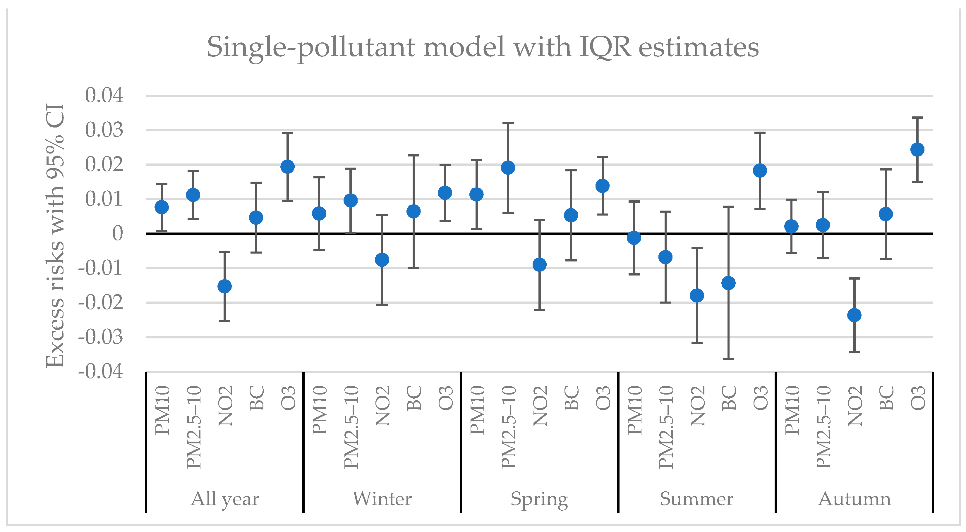
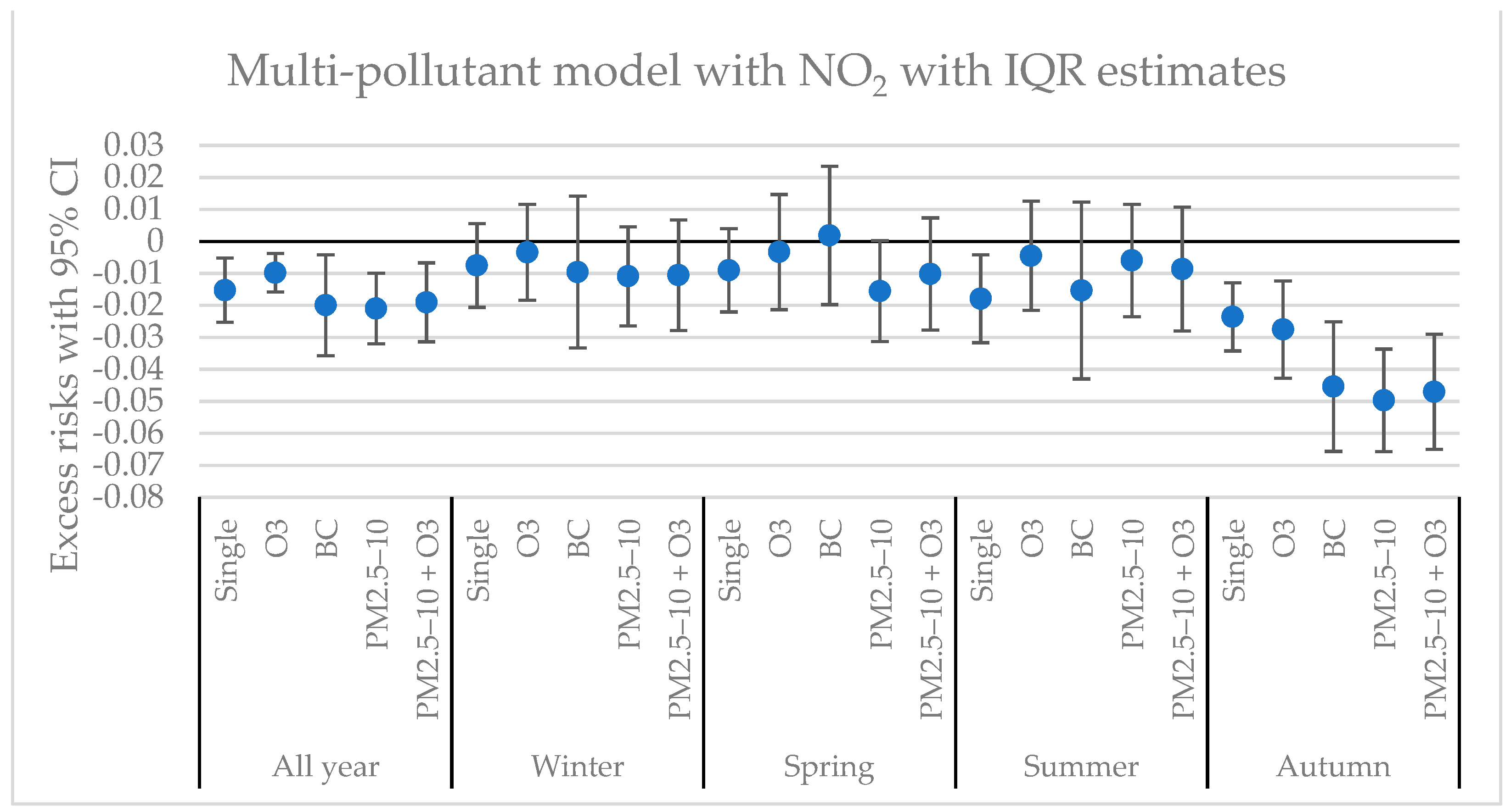
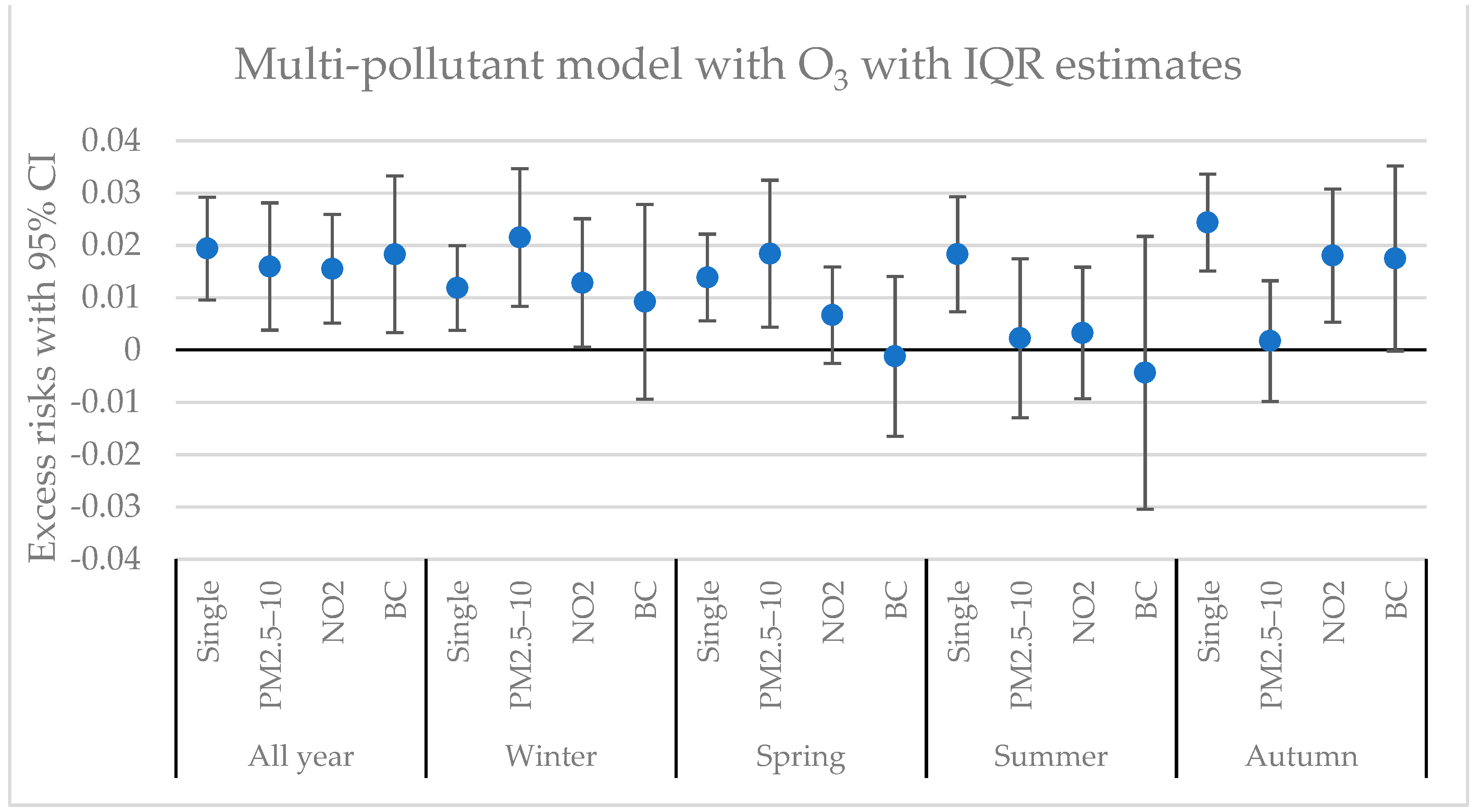
The main objective of this study was to analyze seasonal variations in the excess risks for daily mortality associated with an interquartile range increase in PM10, PM2.5–10, BC, NO2, and O3 in Stockholm during the period from 2000 to 2016. Both single and multi-pollutant models were used in the analysis.
The current study showed a broadly similar pattern for excess risks associated with PM2.5–10 and PM10 with larger risk increases in daily mortality during springtime. The seasonal pattern of the excess risks for PM10 and PM2.5–10 can possibly be explained by the variation in the chemical composition throughout the year, with a larger amount of road dust present during springtime. The excess risks associated with BC were, in most cases, statistically insignificant, which may be due to the fact that the amount of data on which the calculations were based was smaller in comparison with the other air pollutants.
The calculated excess risks for NO2 were negative in almost all cases throughout the whole year. Differences in exposure during the year, which previously was hypothesized as an explanation for the negative excess risks, are unlikely. One possible reason for the negative excess risks associated with NO2 is that the concentrations (on average 14.4 µg m−3) in this study were too low to cause harmful health effects.
The excess risks associated with O3 were most robust in terms of the number of statistically significantly positive relationships, indicating that O3 and its oxidative potential were particularly important in terms of daily mortality associated with air pollution exposure. Higher excess risks were shown during summer and autumn, indicating a higher degree of exposure during the warm seasons.
From a policy point of view, there were clear indications that the health effects associated with exposure to PM2.5–10 and PM10 were most evident during the spring. Additional action strategies to reduce the emissions of road dust particles are, therefore, needed.

Author Contributions

Conceptualization: H.O. (Henrik Olstrup) and B.F.; methodology: H.O. (Henrik Olstrup) and C.Å.; data analysis: H.O. (Henrik Olstrup), C.J., B.F., C.Å., and H.O. (Hans Orru); writing—original draft preparation: H.O. (Henrik Olstrup) and H.O. (Hans Orru); writing—review and editing: C.J., B.F., C.Å. and H.O. (Hans Orru). All authors have read and agreed to the published version of the manuscript.

Funding

This research was partly financed by the Swedish Environmental Protection Agency.

Institutional Review Board Statement

Not applicable.

Informed Consent Statement

Not applicable.

Data Availability Statement

The data presented in this study are available on request from the corresponding author.

Acknowledgments

The authors would like to thank four anonymous reviewers for review and improvement suggestions.

Conflicts of Interest

The authors declare no conflict of interest. The funders had no role in the design of the study; in the collection, analyses, or interpretation of data; in the writing of the manuscript, or in the decision to publish the results.

Appendix A

Table A1. Numbers and percentage of days with valid data for the measured variables during the period from 2000 to 2016 divided into whole year and four different seasons. Mortality is indicated as cases per day, maximum temperature in °C, and air pollutants in µg m−3.
Variable Whole YearWinterSpringSummer Autumn
#Days (% Valid Data)
Mortality 6210 (100%)1535 (100%)1564 (100%)1564 (100%)1548 (100%)
Maximum temperature6210 (100%)1535 (100%)1564 (100%)1564 (100%)1548 (100%)
PM10 5999 (97%)1474 (96%)1533 (98%)1500 (96%)1492 (96%)
PM2.5–105352 (86%)1298 (85%)1378 (88%)1356 (87%)1277 (83%)
BC *3316 (53%)764 (50%) 906 (58%)791 (51%)855 (55%)
NO26101 (98%)1504 (98%)1533 (98%)1527 (98%)1537 (99%)
O36133 (99%)1531 (100%)1553 (99%)1532 (98%)1517 (98%)
* No data available for BC before April 2006.
Table A2. Correlation matrix with R-values (Pearson correlation coefficients) between the different air pollutants measured in Stockholm during the whole year during the period from 2000 to 2016.
PollutantPM10PM2.5–10BCNO2O3
PM1010.810.490.250.31
PM2.5–100.8110.130.120.35
BC0.490.1310.49 −0.25
NO20.250.120.491−0.46
O30.310.35−0.25−0.46 1
Table A3. Correlation matrix with R-values (Pearson correlation coefficients) between the different air pollutants measured in Stockholm during wintertime (December, January and February) during the period from 2000 to 2016.
PollutantPM10PM2.5–10BCNO2O3
PM1010.670.560.24−0.02
PM2.5–100.6710.050.110.13
BC0.560.05 10.48−0.45
NO20.240.110.481−0.62
O3−0.020.13−0.45−0.621
Table A4. Correlation matrix with R-values (Pearson correlation coefficients) between the different air pollutants measured in Stockholm during springtime (March, April and May) during the period from 2000 to 2016.
PollutantPM10PM2.5–10BCNO2O3
PM1010.830.660.460.18
PM2.5–100.8310.310.330.14
BC0.660.3110.54 −0.06
NO20.460.330.541−0.40
O30.180.14−0.06−0.40 1
Table A5. Correlation matrix with R-values (Pearson correlation coefficients) between the different air pollutants measured in Stockholm during summertime (June, July and August) during the period from 2000 to 2016.
PollutantPM10PM2.5–10BCNO2O3
PM1010.710.550.400.44
PM2.5–100.7110.190.160.25
BC0.550.1910.550.11
NO20.400.160.551−0.16
O30.440.250.11−0.161
Table A6. Correlation matrix with R-values (Pearson correlation coefficients) between the different air pollutants measured in Stockholm during autumn time (September, October and November) during the period from 2000 to 2016.
PollutantPM10PM2.5–10BCNO2O3
PM1010.690.690.190.06
PM2.5–100.6910.320.140.12
BC0.690.3210.37−0.30
NO20.190.140.371−0.55
O30.060.12−0.30−0.551

References

  1. Kukkonen, J.; Konttinen, M.; Bremer, P.; Salmi, T.; Saari, H. The seasonal variation of urban air quality in northern European conditions. Int. J. Environ. Pollut. 2000, 14, 480. [Google Scholar] [CrossRef]
  2. Ma, C.; Ding, L. A research on the seasonal difference of air pollution in Chengdu. IOP Conf. Ser. Earth Environ. Sci. 2020, 569, 012071. [Google Scholar] [CrossRef]
  3. Johansson, C.; Norman, M.; Gidhagen, L. Spatial & temporal variations of PM10 and particle number concentrations in urban air. Environ. Monit. Assess. 2007, 127, 477–487. [Google Scholar] [PubMed]
  4. Hoek, G.; Brunekreef, B.; Verhoeff, A.; van Wijnen, J.; Fischer, P. Daily mortality and air pollution in The Netherlands. J. Air Waste Manag. Assoc. 2000, 50, 1380–1389. [Google Scholar] [CrossRef]
  5. Peng, R.D.; Dominici, F.; Pastor-Barriuso, R.; Zeger, S.L.; Samet, J.M. Seasonal Analyses of Air Pollution and Mortality in 100 US Cities. Am. J. Epidemiol. 2005, 161, 585–594. [Google Scholar] [CrossRef]
  6. Nawrot, T.S.; Torfs, R.; Fierens, F.; de Henauw, S.; Hoet, P.H.; van Kersschaever, G.; de Backer, G.; Nemery, B. Stronger associations between daily mortality and fine particulate air pollution in summer than in winter: Evidence from a heavily polluted region in western Europe. J. Epidemiol. Community Health 2007, 61, 146–149. [Google Scholar] [CrossRef] [Green Version]
  7. Läll, K.; Raag, M.; Orru, H. Particulate air pollution and mortality in Tallinn: A time-series analysis in North-Eastern European country. Environ. Health Perspect. 2013, 2013, 4177. [Google Scholar] [CrossRef]
  8. Chen, R.; Peng, R.D.; Meng, X.; Zhou, Z.; Chen, B.; Kan, H. Seasonal variation in the acute effect of particulate air pollution on mortality in the China Air Pollution and Health Effects Study (CAPES). Sci. Total Environ. 2013, 450–451, 259–265. [Google Scholar] [CrossRef] [Green Version]
  9. Qian, Z.; Lin, H.M.; Stewart, W.F.; Kong, L.; Xu, F.; Zhou, D.; Zhu, Z.; Liang, S.; Chen, W.; Shah, N.; et al. Seasonal Pattern of the Acute Mortality Effects of Air Pollution. J. Air. Waste. Manag. Assoc. 2010, 60, 481–488. [Google Scholar] [CrossRef]
  10. Yi, O.; Hong, Y.C.; Kim, H. Seasonal effect of PM10 concentrations on mortality and morbidity in Seoul, Korea: A temperature-matched case-crossover analysis. Environ. Res. 2010, 110, 89–95. [Google Scholar] [CrossRef]
  11. Lyon, J.L.; Mori, M.; Gao, R. Is there a causal Association between Excess Mortality and Exposure to PM-10 air Pollution? Additional Analyses by Location, year, Season, and Cause of Death. Inhal. Toxicol. 1995, 7, 603–614. [Google Scholar] [CrossRef]
  12. Hsu, W.H.; Hwang, S.A.; Kinney, P.L.; Lin, S. Seasonal and temperature modifications of the association between fine particulate air pollution and cardiovascular hospitalization in New York State. Sci. Total Environ. 2017, 578, 626–632. [Google Scholar] [CrossRef] [Green Version]
  13. Meister, K.; Johansson, C.; Forsberg, J. Estimated short-term effects of coarse particles on daily mortality in Stockholm, Sweden. Environ. Health Perspect. 2012, 120, 431–436. [Google Scholar] [CrossRef] [PubMed] [Green Version]
  14. Duan, Y.; Liu, X.; Li, H.; Yan, S.; Yan, M.; Mang, Y.; Yin, P. Season and temperature modify the short-term effect of nitrogen dioxide on cardiovascular mortality: A time-series study. Lancet 2019, 394, S57. [Google Scholar] [CrossRef]
  15. Liu, T.; Zeng, W.; Lin, H.; Rutherford, S.; Xiao, J.; Li, X.; Li, Z.; Qian, Z.; Feng, B.; Ma, W. Tempo-Spatial Variations of Ambient Ozone-Mortality Associations in the USA: Results from the NMMAPS Data. Int. J. Environ. Res. Public Health 2016, 13, 851. [Google Scholar] [CrossRef] [PubMed] [Green Version]
  16. Pascal, M.; Wagner, V.; Chatignoux, E.; Falq, G.; Corso, M.; Blanchard, M.; Host, S.; Larrieu, S.; Pascal, L.; Declercq, C. Ozone and short-term mortality in nine French cities: Influence of temperature and season. Atmos. Environ. 2012, 62, 566–572. [Google Scholar] [CrossRef]
  17. Qin, L.; Gu, J.; Liang, S.; Fang, F.; Bai, W.; Liu, X.; Zhao, T.; Walline, J.; Zhang, S.; Cui, Y.; et al. Seasonal association between ambient ozone and mortality in Zhengzhou, China. Int. J. Biometeorol. 2017, 61, 1003–1010. [Google Scholar] [CrossRef]
  18. Olstrup, H.; Johansson, C.; Forsberg, B.; Åström, C. Association between Mortality and Short-Term Exposure to Particles, Ozone and Nitrogen Dioxide in Stockholm, Sweden. Int. J. Environ. Res. Public Health 2019, 16, 1028. [Google Scholar] [CrossRef] [Green Version]
  19. Auger, N.; Potter, B.J.; Smargiassi, A.; Bilodeau-Bertrand, M.; Paris, C.; Kosatsky, T. Association between quantity and duration of snowfall and risk of myocardial infarction. CMAJ 2017, 189, E235–E242. [Google Scholar] [CrossRef] [PubMed] [Green Version]
  20. Norman, M.; Johansson, C. Studies of some measures to reduce road dust emissions from paved roads in Scandinavia. Atmos. Environ. 2006, 40, 6154–6164. [Google Scholar] [CrossRef]
  21. Khan, R.K.; Strand, M.A. Road dust and its effect on human health: A literature review. Epidemiol. Health 2018, 40, e2018013. [Google Scholar] [CrossRef] [PubMed]
  22. Krecl, P.; Targino, A.C.; Johansson, C. Spatiotemporal distribution of light-absorbing carbon and its relationship to other atmospheric pollutants in Stockholm. Atmos. Chem. Phys. 2011, 11, 11553–11567. [Google Scholar] [CrossRef] [Green Version]
  23. Bedada, G.B.; Raza, A.; Forsberg, B.; Lind, T.; Ljungman, P.; Pershagen, G.; Bellander, T. Short-term exposure to ozone and mortality in subjects with and without previous cardiovascular disease. Epidemiology 2016, 27, 663–669. [Google Scholar] [CrossRef] [PubMed]
  24. Samoli, E.; Aga, E.; Touloumi, G.; Nisiotis, K.; Forsberg, B.; Lefranc, A.; Pekkanen, J.; Wojtyniak, B.; Schindler, C.; Niciu, E.; et al. Short-term effects of nitrogen dioxide on mortality: An analysis within the APHEA project. Eur. Respir. J. 2006, 27, 1129–1138. [Google Scholar] [CrossRef] [PubMed]
  25. Kraft, M.; Eikmann, T.; Kappos, A.; Künzli, N.; Rapp, R.; Schneider, K.; Seitz, H.; Voss, J.U.; Wichmann, H.E. The German view: Effects of nitrogen dioxide on human health–derivation of health-related short-term and long-term values. Int. J. Hyg. Environ. Health 2005, 208, 305–318. [Google Scholar] [CrossRef]
  26. Ritz, B.; Hoffmann, B.; Peters, A. The Effects of Fine Dust, Ozone, and Nitrogen Dioxide on Health. Dtsch. Arztebl. Int. 2019, 116, 881–886. [Google Scholar] [CrossRef]
  27. Meng, X.; Liu, C.; Chen, R.; Sera, F.; Vicedo-Cabrera, A.M.; Milojevic, A.; Guo, Y.; Tong, S.; Coelho, M.D.; Saldiva, P.H.; et al. Short term associations of ambient nitrogen dioxide with daily total, cardiovascular, and respiratory mortality: Multilocation analysis in 398 cities. BMJ. 2021, 372, n534. [Google Scholar] [CrossRef]
  28. Lavigne, E.; Burnett, R.T.; Weichenthal, S. Association of short-term exposure to fine particulate air pollution and mortality: Effect modification by oxidant gases. Sci. Rep. 2018, 8, 16097. [Google Scholar] [CrossRef]
  29. Zhang, Z.; Weichenthal, S.; Kwong, J.C.; Burnett, R.T.; Hatzopoulou, M.; Jerrett, M.; Donkelaar, A.V.; Bai, L.; Martin, R.V.; Copes, R.; et al. Long-term exposure to iron and copper in fine particulate air pollution and their combined impact on reactive oxygen species concentration in lung fluid: A population-based cohort study of cardiovascular disease incidence and mortality in Toronto, Canada. Int. J. Epidemiol. 2021, 50, 589–601. [Google Scholar] [CrossRef]
Figure 1. Estimated excess risks in daily mortality with 95% CI (lag02) for an IQR increase in the concentrations of PM10, PM2.5–10, NO2, BC and O3 in single-pollutant models divided into all year and four different seasons.
Atmosphere 12 01481 g001
Figure 2. Estimated excess risks in daily mortality with 95% CI (lag02) for an IQR increase in the concentrations of PM10. The calculations are divided into all year and four different seasons. The excess risks are presented as single-pollutant estimates and multi-pollutant estimates with O3, NO2 and NO2 + O3 included in the calculations.
Atmosphere 12 01481 g002
Figure 3. Estimated excess risks in daily mortality with 95% CI (lag02) for an IQR increase in the concentrations of PM2.5–10. The calculations are divided into all year and four different seasons. The excess risks are presented as single-pollutant estimates and multi-pollutant estimates with O3, NO2 and NO2 + O3 included in the calculations.
Atmosphere 12 01481 g003
Figure 4. Estimated excess risks in daily mortality with 95% CI (lag02) for an IQR increase in the concentrations of BC. The calculations are divided into all year and four different seasons. The excess risks are presented as single-pollutant estimates and multi-pollutant estimates with O3, NO2 and NO2 + O3 included in the calculations.
Atmosphere 12 01481 g004
Figure 5. Estimated excess risks in daily mortality with 95% CI (lag 02) for an IQR increase in the concentrations of NO2. The calculations are divided into all year and four different seasons. The excess risks are presented as single-pollutant estimates and multi-pollutant estimates with O3, BC, PM2.5–10 and PM2.5–10 + O3 included in the calculations.
Atmosphere 12 01481 g005
Figure 6. Estimated change in daily mortality with 95% CI (lag02) for an IQR increase in the concentrations of O3. The calculations are divided into all year and four different seasons. The excess risks are divided into single-pollutant estimates and multi-pollutant estimates with PM2.5–10, NO2 and BC included in the calculations.
Atmosphere 12 01481 g006
Table 1. Measurement methods and instruments used to measure the pollutants.
PollutantMethodInstrument
PM10GravimetricTEOM 1400A, Thermo Fisher Scientific, Waltham, MA, USA
PM2.5GravimetricTEOM 1400A, Thermo Fisher Scientific, Waltham, MA, USA
PM2.5–10Gravimetric
(Subtracting PM2.5 from PM10)
TEOM 1400A, Thermo Fisher Scientific, Waltham, MA, USA
BCTransmission of lightthrough a filterAethalometers 8100, AE31, AE33,
Magee Scientific Corporation, Berkeley, CA, USA
NO2ChemiluminescenceAC32M, Environnement S.A., Poissy, France
O3UV absorptionO342M, Environnement S.A., Poissy, France
Table 2. Summary statistics of the daily data from 2000 to 2016 during whole year and in four different seasons.
VariableWhole YearWinterSpringSummerAutumn
Mean (IQR)
Mortality (cases per day)18.5 (7.0)20.2 (6.0)18.7 (6.0)17.0 (6.0)17.9 (6.0)
Maximum temperature (°C)11.4 (15.0)1.4 (5.6)10.9 (9.8)22.2 (5.0)11.0 (8.3)
PM10 (µg m−3)14.5 (8.7)12.2 (7.7)20.5 (13.7)12.9 (5.9)12.2 (6.7)
PM2.5–10 (µg m−3)8.0 (5.5)5.5 (3.7)13.1 (10.8)6.8 (3.8)6.3 (3.8)
BC (µg m−3)0.6 (0.5)0.7 (0.6)0.6 (0.4)0.5 (0.5)0.7 (0.5)
NO2 (µg m−3)14.4 (9.9)17.6 (11.5)14.0 (9.4)10.8 (7.4)15.2 (9.6)
O3 (µg m−3) *51.2 (25.2)41.6 (20.1)66.1 (17.4)58.0 (17.5)38.8 (18.0)
* O3 measurements were based on daily maximum 8-h mean values.
Publisher’s Note: MDPI stays neutral with regard to jurisdictional claims in published maps and institutional affiliations.

