Temporal Variability of Drought in Nine Agricultural Regions of China and the Influence of Atmospheric Circulation

Abstract

In recent decades, the severe drought across agricultural regions of China has had significant impact on agriculture. The standardized precipitation evapotranspiration index (SPEI) has been widely used for drought analyses; however, SPEI is prone to be affected by potential evapotranspiration (PET). We thus examined the correlations between soil moisture anomalies and the SPEI calculated by the Thornthwaite, Hargreaves, and Penman–Monteith (PM) equations to select the most suitable for drought research. Additionally, the Mann–Kendall and wavelet analysis were used to investigate drought trends and to analyze and the impact of atmospheric circulation on drought in China from 1961 to 2018. The results showed that (1) PET obtained from the PM equation is the most suitable for SPEI calculation; (2) there were significant wetting trends in Northern China and the whole Chinese mainland and most of the wetting mutation points occurred in the 1970s and 1980s and the significant inter-annual oscillations period in the Chinese mainland was 2–4 years; (3) the Chinese mainland and Northern China are strongly influenced by West Pacific Trade Wind, while Western Pacific Subtropical High Intensity and Pacific Subtropical High Area have primary impact on Southern China.

1. Introduction

Drought is considered one the most devastating disasters and can affect a host of economic and social activities [1]. Drought adversely impacts both surface and groundwater resources, with effects including reduction of water supply, water quality deterioration, crop failure, vegetation productivity loss, hydropower generation decrease, and riparian habitat destruction [2,3,4,5,6]. Furthermore, some developing regions disproportionately affected by droughts have poor ability to cope with drought, which increases wealth inequality between the rich and the poor [7]. Due to the severe consequences of drought, it is critical to assess the variability of drought and determine the most influential contributing factors.

To monitor and analyze drought, many indices have been developed [8,9]; these include the Standardized Precipitation Index (SPI) [10], Standardized Antecedent Precipitation Evapotranspiration Index (SAPEI) [11], and Standardized Precipitation Evapotranspiration Index (SPEI) [12]. SPI has a wide range of application due to its simple calculation and the easily accessible input data—that is, precipitation. However, this simplicity has advantages and disadvantages. The application of SPI in semi-arid and arid regions is often limited by the fact that it only considers precipitation and neglects other factors such as temperature and evapotranspiration that play an important role in drought monitoring [13,14,15]. The SPEI is regarded as one of the most reliable to identify drought as it comprises both precipitation and evapotranspiration, parameters that significantly impact drought [16,17,18,19]. In addition, one crucial advantage of the SPEI over other widely used drought indices that consider PET is that its multi-scalar characteristics enable it to identify different drought types and their effects in the context of global warming [15]. Therefore, compared with SPI, the SPEI is the most suitable for the study of drought in the Chinese mainland, which exhibits a variety of climate types. The SPEI is more sensitive to changes in potential evapotranspiration (PET) than other parameters, especially in arid regions such as the Sahara and Middle East [20,21,22]. PET is the most important variable to consider when using the SPEI for drought analyses. The SPEI can return significant conflicting results regarding changes in drought due to differences between calculations of PET; these different calculations include the simple Thornthwaite (TH) equation, the Hargreaves (HS) equation, and the Penman–Monteith (PM) equation [12,23].

Recent studies have compared the effects of different PET equations on drought indices. For example, Van der Schrier et al. [24] and Dai [25] compared the effects of using the TH and PM equations for PET to obtain the Palmer Drought Severity Index (PDSI) on a global scale and reported no difference in the resulting PDSI trends. However, Sheffield et al. [26] reviewed these studies and argued that errors in the forcing data or the calibration period were sufficient to explain why no differences were found and concluded that there were in fact large differences in the PDSI when using either the TH or PM equations for PET. In fact, they saw that the two approaches disagreed in the sign of the trends across America, Eastern sub-Saharan Africa, Western Russia, Southeast Asia, and Australia. In regions that are water-limited, the actual evaporation is small, and therefore the impact of PET on the PDSI is also small. However, in energy-limited regions, the differences in PET can translate into large differences, even changing the sign of the PDSI trends. Begueria et al. [17] compared the effect of using the TH, HS, and PM equations for PET when calculating the SPEI (SPEI_th, SPEI_hs, and SPEI_pm) at the global scale. They postulated that the magnitude of the differences between the SPEI series based on different PET equations might be related to the weight that the different equations give to precipitation relative to the climatic water balance at each site; at the global scale, all three PET equations returned downward trends, but the trends from SPEI_th and SPEI_pm were stronger than that from SPEI_hs. In general, these differences were more pronounced in semi-arid to mesic areas and less pronounced in humid regions. Clearly, the equations used to calculate PET can greatly influence the SPEI [17,27,28].

The PM equation has been recommended as the sole standard method for the computation of PET by Food and Agriculture Organization (FAO) [29]. It is physically based and explicitly incorporates both physiological and meteorological parameters. In the context of global climate change, other climate variables can also produce changes in drought and the temperature-based TH and HS are not as accurate as PM when data are abundant. Therefore, because the PM equation considers more meteorological factors and physical mechanisms, it is preferred when calculating SPEI. Where data quality is questionable, or where historical data are missing, HS is commonly recommended because it is surprisingly comparable to PM over a wide range of climates [30]. Due to data limitations, the TH equation is most widely used because it only considers temperature, and this makes TH the most primitive equation for calculating PET. It has been widely used because its calculation principle is simple and requires less data, and it still effectively reflects changes in evapotranspiration, especially in arid and semi-arid areas [17,25,31]. However, due to the large number of input variables (e.g., wind speed, relative humidity, and radiation), there are some uncertainties in the calculation of the PM equation [17]. Thus, the effect of using different PET equations for calculation of drought indices remains an open question.

As China has suffered several prolonged and severe droughts in recent decades, such as the 2009–2010 drought in Southwest China, Eastern China drought during 2013, and North China drought in 2014 [32,33], the study of drought has received increasing attention. Yu et al. [18] investigated the dryness/wetness cycles in China using the SPEI calculated with the TH equation and found that a significant trend toward drier conditions was present in most of China. However, Wang et al. [34] used the self-calibrating Palmer Drought Severity Index (scPDSI), obtained with the PM equation, to show that China experienced an increasing wetness trend at both the annual and seasonal scales. The differences in drought trends may be closely related to the indices used and use of different equations to calculate PET [18,33]. China has a diverse climate and the most suitable PET equation may be different for different regions [35]. Therefore, it is essential to use the appropriate PET methods for drought analyses in different climatic regions [20]. However, few studies have attempted to identify the most suitable PET equation for calculating the SPEI for different agricultural regions in China.

In addition, the availability of water resources in China is strongly influenced by climatic conditions. Fluctuations in water resource availability are often linked to anomalous atmospheric conditions, as they can increase or decrease rainfall and affect key parameters (e.g., temperature, soil moisture, and evaporation) of the hydrological cycle which significantly influence the occurrence of droughts [1,36,37,38,39]. For instance, El Niño-Southern Oscillation (ENSO) is the strongest inter-annual signal of the coupled air–sea system in the tropical Pacific. It not only impacts the oceanic parameters within the Pacific but also influences the climate of areas bordering the Pacific, as well as the global climate [40]. Wang et al. [41] revealed that ENSO events had a strong influence on regional precipitation in the Yellow River Basin of China, resulting in a 51% decrease in runoff to the sea. Zhang et al. [42] reported an (in-phase or antiphase) interconnection between ENSO and the annual maximum streamflow from the upper to the lower Yangtze River Basin. These studies demonstrated that large-scale atmospheric circulation factors have a strong influence on the climate of China. However, the dominant atmospheric circulation indices that affect drought in each agricultural region of China remain unclear. Furthermore, relatively few studies have analyzed the relationships between drought and atmospheric circulation factors for different agricultural regions in China.

Therefore, the objectives of this study were to (1) select the most suitable PET formula to calculate SPEI, (2) to determine the drought trends and periodic features in different agricultural regions of China, and (3) to deduce the relationships between atmospheric circulation factors and drought. This study deepened our understanding of historical drought events in different agricultural regions of China and provided a scientific basis for the management of future agriculture water resources.

2. Study Area and Data

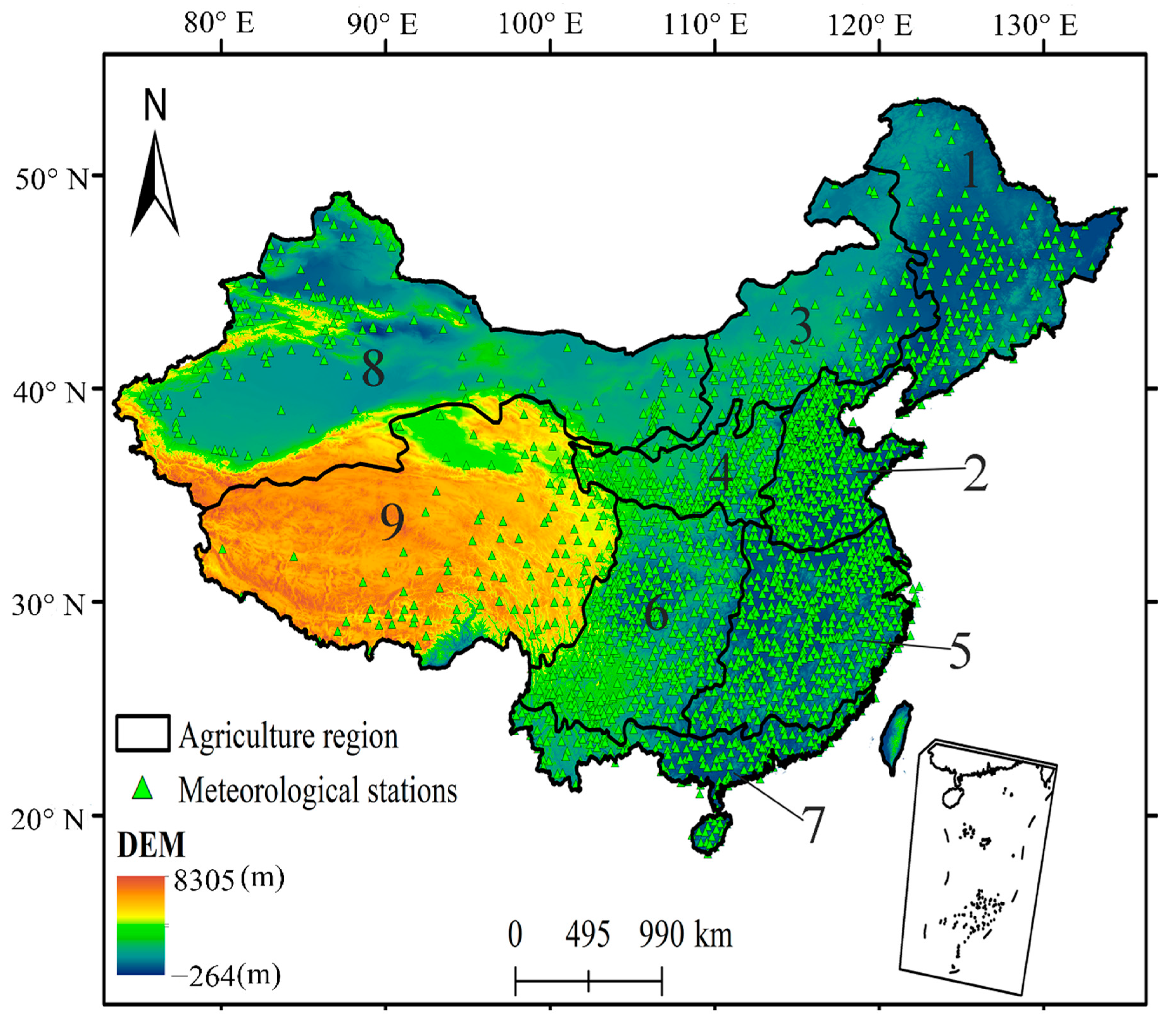
2.1. Study Area

The Chinese mainland (Figure 1) was selected as the study area. It is located in Eastern Asia on the west coast of the Pacific Ocean and has an area of around 9.6 million square kilometers. The Chinese mainland exhibits strong monsoon and continental climate characteristics. China is topographically diverse, with higher altitudes in the west and lower in the east, with a roughly three step distribution [43]. A temperate continental climate dominates the northwest region, and a temperate monsoon climate dominates in the northeast region. A subtropical monsoon climate prevails in Southern China, except for the southernmost region, where a tropical monsoon climate is dominant. The Qinghai-Tibetan Plateau is dominated by a plateau alpine climate. The majority of the Chinese mainland is located within the East Asian monsoon region and experiences significant monthly, annual, and inter-annual variation in temperature and precipitation. The temperature differences between the north and the south of China varies widely [44]. The distribution of precipitation during the year is uneven in space and time, and droughts and floods are frequent. In most areas, the more than 70% of annual precipitation is concentrated into four consecutive months, with continuous wet or dry spells being more common. The regional distribution of water resources in China is also very uneven [45]. For example, the land area of the Yangtze River Basin and its southern region only accounts for 36.5% of the country, but its water resources account for 81% of the country’s water. The land area in the northern region accounts for 63.5% of the country, but it has only 19% of the country’s water resources [34,46].

To fully analyze droughts, this study divided China into nine agricultural regions according to the study by Xu et al. [47]. The nine agricultural regions included (1) Northeast China Region (NECR); (2) Huang-Huai-Hai Region (HHHR); (3) Inner Mongolia and the Great Wall Region (MGR); (4) Loess Plateau Region (LPR); (5) middle and lower regions of the Yangtze River (YRR); (6) Southwest China Region (SWCR); (7) South China Region (SCR); (8) Gan-Xin Region (GXR); (9) Qinghai-Tibet Plateau Region (QTR).

2.2. Data

The monthly meteorological data used in this study spanned from 1961 to 2018 and included precipitation (PRE), mean temperatures (TEM), maximum air temperature (TMAX), minimum air temperature (TMIN), wind speed (WIN), atmospheric pressure (PRS), relative humidity (RH), and sunshine duration (SSD). The climate data, except for the radiation data, were derived from 2417 climatological stations distributed throughout the Chinese mainland. All data were provided by the China Meteorological Administration [48]. To ensure the quality of the data, we validated these data by screening and eliminating suspicious and missing records. Inverse distance weighting (IDW) is a widely used method for multivariate interpolation with a known scattered set of points and is reliable to create gridded climate data for China [22,23]. We thus used the IDW to interpolate site data to a resolution of 0.5°. In addition, the 0.25° daily root zone (0–100 cm) soil moisture (SM) dataset obtained from the Community Land Model (CLM) of the Global Land Data Assimilation System (GLDAS) [49] was also used when selecting the most suitable PET equation for calculating the SPEI. The dataset from 1961 to 2014 was downloaded from the Goddard Earth Sciences Data and Information Services Center [50]. To ensure matching spatial scales, the GLDAS soil moisture dataset was resampled to 0.5° using bilinear interpolation. In order to avoid the effect of seasonality, it was then transformed as the soil moisture standardized anomaly (SMA) according to

$$SM{A}_{i,j}=\frac{S{M}_{i,j}-\overline{S{M}_j}}{{\sigma }_j},$$

(1)

where i represents year ranging from 1961 to 2014 and j the month ranging from January to December, $SM{A}_{i,j}$ stands for the standardized soil moisture anomalies for month j and year i, $S{M}_{i,j}$ means the soil moisture value in month j and year i, $S{M}_j$ and ${\sigma }_j$ illustrate the average value and standard deviation of the soil moisture for month j, respectively. The GLDAS CLM soil moisture dataset has been found to be capable of capturing the dry and wet conditions in China [51,52].

The circulation indices included 88 circulation parameters. The 88 monthly circulation parameters (January 1961 to December 2018) were obtained from the Climate Diagnostics and Prediction Division of the National Climate Center of China [53].

3. Methodology

The flowchart of the methodology used in this study is depicted in Figure 2.

3.1. PET Calculation Methods

The PET is a climatic parameter that expresses the evaporative power of the atmosphere. It represents the evapotranspiration rate from a reference surface with an unlimited supply of water. Considering the applicability of each equation and their data requirements, three PET equations were considered: the TH equation, HS equation, and PM equation.

3.1.1. TH Equation

The Thornthwaite equation (TH) [54] is the most basic of the formulas for calculating PET, but it has the advantage of requiring only monthly mean temperature data. Following this method, the monthly PET (mm) is obtained by

$$\mathrm{PET}=16{\left(\frac{10\mathrm{T}}{\mathrm{I}}\right)}^{\mathrm{m}},$$

(2)

where T is averaged monthly temperature; m is a coefficient depending on I: $\mathrm{m}=6.75\times {10}^{-7}{\mathrm{I}}^3-7.71\times {10}^{-5}{\mathrm{I}}^2+1.79\times {10}^{-2}\mathrm{I}+0.492$; I is a heat index, which is the sum of the 12 monthly index values i, which are in turn derived from mean monthly temperatures using the formula

$$\mathrm{i}={\left(\frac{\mathrm{T}}{5}\right)}^{1.514}$$

(3)

3.1.2. HS Equation

The Hargreaves equation (HS) [55] can be used to calculate PET for weekly periods or longer. The attractiveness of this method is its simplicity, reliability, minimal data requirements, ease of computation, and low impact of weather station aridity. It is calculated as follows:

$$\mathrm{PET}=0.0135{\mathrm{C}}_{\mathrm{HS}}\frac{{\mathrm{R}}_{\mathrm{a}}}{\mathsf{\lambda }}\left(\mathrm{T}+17.8\right)\cdot {\left({\mathrm{T}}_{\max }-{\mathrm{T}}_{\min }\right)}^{0.5},$$

(4)

$${\mathrm{C}}_{\mathrm{HS}}=0.00185{\left({\mathrm{T}}_{\max }-{\mathrm{T}}_{\min }\right)}^2-0.0433\left({\mathrm{T}}_{\max }-{\mathrm{T}}_{\min }\right)+0.4023,$$

(5)

${\mathrm{R}}_{\mathrm{a}}$ is the extraterrestrial solar radiation (MJ/m²); λ is the latent heat of vaporization (MJ/kg); T, ${\mathrm{T}}_{\max }$ and ${\mathrm{T}}_{\min }$ are the mean, daily max, and daily min air temperatures.

3.1.3. PM Equation

The Penman–Monteith equation (PM) [29] is based on numerous physical parameters and is widely used for estimating PET. Compared with the TH and HS, the PM requires more variables but can more realistically simulate PET [24]. The PM method has been recommended as the sole standard method for the computation of PET by the FAO. The PM equation is

$$\mathrm{PET}=\frac{0.408\Delta \left({\mathrm{R}}_{\mathrm{n}}-\mathrm{G}\right)+\mathsf{\gamma }\left(\frac{900}{\mathrm{T}+273}\right)\cdot {\mathrm{u}}_2\cdot \left({\mathrm{e}}_{\mathrm{s}}-{\mathrm{e}}_{\mathrm{a}}\right)}{\Delta +\mathsf{\gamma }\left(1+0.34{\mathrm{u}}_2\right)},$$

(6)

where $\Delta$ is the slope of vapor pressure curve (kPa/°C); γ is the psychrometric constant (kPa/°C); ${\mathrm{R}}_{\mathrm{n}}$ is the net incoming radiation at the evaporative surface (MJ/m²); G is the soil heat flux (MJ/m²); T is the mean air temperature; ${\mathrm{u}}_2$ is the wind speed at a height of 2 m; ${\mathrm{e}}_{\mathrm{s}}$ and ${\mathrm{e}}_{\mathrm{a}}$ are the saturated and actual vapor pressures. The details of the parameters above can be found in a previously published paper of Guo et al. [56].

3.2. SPEI

The SPEI was constructed by Vicente-Serrano et al. [12]. Based on the standardized precipitation index (SPI), the SPEI introduced potential evapotranspiration. This index takes into account the step-by-step law of precipitation statistics but also considers evapotranspiration over the same period, which more comprehensively reflects drought situations across different climates. The SPEI value indicates the degree of dryness or wetness, with larger values indicating wetter situations and smaller values indicating drier.

Table 1. Categorization of dryness/wetness grade by the SPEI.

Categories	SPEI Values
Extremely dryness	Less than −2
Severe dryness	−1.99 to −1.5
Moderate dryness	−1.49 to −1.0
Near normal	−1.0 to 1.0
Moderate wetness	1.0 to 1.49
Severe wetness	1.50 to 1.99
Extremely wetness	More than 2

shows the corresponding drought classifications. The detailed calculation of the SPEI is described in the study by Vicente-Serrano et al. [12].

3.3. Continuous Wavelet Transform (CWT)

The CWT, introduced by Torrence and Compo [57], has been widely used to study the periodicity of droughts [38,40,58]. Of the many wavelet functions, the Morlet wavelet function has been shown to have a good balance between time and frequency localizations and is thus preferred.

The CWT decomposes a time series over a temporal-scale space, identifying the dominant modes of variability and their variation characteristics over time [59]. The wavelet function $\mathsf{\psi }\left(\mathrm{t}\right)$ can be defined as

$$\mathrm{E}{{\displaystyle \int }}_{-\infty }^{+\infty }\mathsf{\psi }\left(\mathrm{t}\right)\mathrm{dt}=0,$$

(7)

where $\mathsf{\psi }\left(t\right)$ is a special type of waveform that has finite length and a zero mean value [60]. These features are suitable for the analysis of non-stationary processes that contain multi-scale features [57]. The CWT of the discrete time series ${\mathrm{x}}_{\mathrm{t}}=\left(\mathrm{t}=0,\dots \dots \mathrm{t}-1\right)$ can be defined as the convolution of ${\mathrm{x}}_{\mathrm{t}}$ with a scaled and translated version of ${\mathsf{\psi }}_0\left(\mathsf{\eta }\right)$:

$${\mathrm{W}}_{\mathrm{t}}^{\mathrm{x}}\left(\mathrm{s}\right)=\sqrt{\frac{\Delta \mathrm{t}}{\mathrm{s}}}{{\displaystyle \sum }}_{\mathrm{t}=1}^{\mathrm{n}}{\mathrm{x}}_{\mathrm{t}}{\mathsf{\psi }}_0^{*}\left(\frac{\left(\mathrm{t}-\mathrm{i}\right)\Delta \mathrm{t}}{\mathrm{s}}\right),$$

(8)

where W is the wavelet coefficient; s is the scale factor that determines the degree of compression or scale; $\Delta \mathrm{t}$ is the time step; ${\mathsf{\psi }}_0^{*}$ denotes the complex conjugate of ${\mathsf{\psi }}_0$. In this study, we used the complex non-orthogonal Morlet wavelet as the mother function because it is reasonably well localized in both the time and frequency domains [61]. The Morlet wavelet function $\left({\mathsf{\psi }}_0\left(\mathrm{t}\right)\right)$ is expressed as follows:

$${\mathsf{\psi }}_0\left(\mathrm{t}\right)={\mathsf{\pi }}_{\mathrm{X}}^{-1/4}{\mathrm{e}}^{{\mathrm{i}\mathsf{\omega }}_0\mathrm{t}}{\mathrm{e}}^{-1/4{\mathrm{t}}^2},$$

(9)

where $\mathrm{t}$ is dimensionless time and ${\mathsf{\omega }}_0$ is dimensionless frequency. Because the wavelet is not completely localized in time, the CWT has an edge artifact problem [54]. To resolve this, a cone of influence (COI) is employed [59]. The COI is the region outside the concave-up shaped area [60]. Thus, the wavelet power ${\left|{\mathrm{W}}_{\mathrm{t}}^{\mathrm{x}}\left(\mathrm{s}\right)\right|}^2$ caused by the discontinuity at the edge is dropped to ${\mathrm{e}}^{-2}$ of the value at the edge [61,62].

3.4. Cross-Wavelet Transform (XWT)

Cross-wavelet transform can be used to analyze the coherence of the CWT in time frequency space and thus to determine the intensity of the covariance of the two time series [63].

The cross-wavelet transform of two time series ${\mathrm{x}}_{\mathrm{n}}$ and ${\mathrm{y}}_{\mathrm{n}}$ is defined as ${\mathrm{W}}^{\mathrm{XY}}={\mathrm{W}}^{\mathrm{X}}{\mathrm{W}}^{\mathrm{Y}*}$, where * denotes a complex conjugation. We further define the cross-wavelet power as $\left|{\mathrm{W}}^{\mathrm{XY}}\right|$. The complex argument arg(${\mathrm{W}}^{\mathrm{xy}}$) can be interpreted as the local relative phase between ${\mathrm{x}}_{\mathrm{n}}$ and ${\mathrm{y}}_{\mathrm{n}}$ in time frequency space. The theoretical distribution of the cross-wavelet power of two time series with background power spectra ${\mathrm{P}}_{\mathrm{k}}^{\mathrm{X}}$ and ${\mathrm{P}}_{\mathrm{k}}^{\mathrm{Y}}$ was published by Torrence and Compo [57] as

$$\mathrm{D}\left(\frac{\left|{\mathrm{W}}_{\mathrm{n}}^{\mathrm{X}}\left(\mathrm{s}\right){\mathrm{W}}_{\mathrm{n}}^{\mathrm{Y}\ast }\left(\mathrm{s}\right)\right|}{{\mathsf{\sigma }}_{\mathrm{X}}{\mathsf{\sigma }}_{\mathrm{Y}}}<\mathrm{p}\right)=\frac{{\mathrm{Z}}_{\mathrm{v}}\left(\mathrm{p}\right)}{\mathrm{v}}\sqrt{{\mathrm{P}}_{\mathrm{k}}^{\mathrm{X}}{\mathrm{P}}_{\mathrm{k}}^{\mathrm{Y}}},$$

(10)

where ${\mathrm{Z}}_{\mathrm{v}}\left(\mathrm{p}\right)$ is the confidence level associated with the probability p for a pdf defined by the square root of the product of the two ${\mathsf{\chi }}^2$ distributions.

3.5. Mann–Kendall (MK) Test

The MK test was proposed separately by both Mann [64] and Kendall [65] and has been widely used for trend analysis of time series [19]. In addition, MK can also be used in change point detection.

For trend analyses, in the Mann–Kendall test, the null hypothesis ${\mathrm{H}}_0$ states that ${\mathrm{X}}_1$, …, ${\mathrm{X}}_{\mathrm{n}}$ are samples of n independent and identically distributed random variables with no seasonal change. The alternative hypothesis ${\mathrm{H}}_1$ for a two-sided test defines the distributions of ${\mathrm{X}}_{\mathrm{k}}$ and ${\mathrm{X}}_{\mathrm{j}}$ as non-identical for all k, j $\le$ n with k $\ne$ j. The test statistic S, with zero mean and computed variance (as in Equation (13)), is asymptotically normal and can be calculated following the Equations (11) and (12):

$$\mathrm{S}={\displaystyle \sum }_{\mathrm{k}=1}^{\mathrm{n}-1}{\displaystyle \sum }_{\mathrm{j}=\mathrm{k}+1}^{\mathrm{n}}\mathrm{sgn}\left({\mathrm{x}}_{\mathrm{j}}-{\mathrm{x}}_{\mathrm{k}}\right)$$

(11)

$$\mathrm{sgn}\left({\mathrm{X}}_{\mathrm{j}}-{\mathrm{X}}_{\mathrm{k}}\right)=\left\{\begin{array}{c}+1 \mathrm{if}\left({\mathrm{X}}_{\mathrm{j}}-{\mathrm{X}}_{\mathrm{k}}\right)>0\\ 0 \mathrm{if}\left({\mathrm{X}}_{\mathrm{j}}-{\mathrm{X}}_{\mathrm{k}}\right)=0\\ -1 \mathrm{if}\left({\mathrm{X}}_{\mathrm{j}}-{\mathrm{X}}_{\mathrm{k}}\right)<0\end{array}\right\}$$

(12)

$$\mathrm{Var}\left(\mathrm{S}\right)=\left[\mathrm{n}\left(\mathrm{n}-1\right)\left(2\mathrm{n}-5\right)-{\displaystyle \sum }_{\mathrm{t}}\mathrm{t}\left(\mathrm{t}-1\right)\left(2\mathrm{t}+5\right)/18\right]$$

(13)

The notation t is the extent of the given time and ∑ denotes the summation over the time span. In cases where the sample size n > 10, the standard normal variate Z is computed:

$$\mathrm{Z}=\left\{\begin{array}{c}\frac{\mathrm{S}-1}{\sqrt{\mathrm{Var}\left(\mathrm{S}\right)}} \mathrm{if} S>0\\ 0 \mathrm{if} S=0\\ \frac{\mathrm{S}+1}{\sqrt{\mathrm{Var}\left(\mathrm{S}\right)}} \mathrm{if} S<0\end{array}\right\}$$

(14)

A positive Z value indicates an ‘upward-trend’ while a negative Z value indicates a ‘downward-trend’ [19].

The sequential version of Mann–Kendall test is used to test assumptions about the start of a trend within the sample ${\mathrm{X}}_1$, …, ${\mathrm{X}}_{\mathrm{n}}$ from set of random variables X based on rank series of progressive and retrograde rows of the sample. The magnitudes of ${\mathrm{X}}_{\mathrm{j}}$ annual mean time series and j = 1,..., n are compared by ${\mathrm{X}}_{\mathrm{k}}$, where k = 1,..., j − 1. For each comparison, the number of cases ${\mathrm{X}}_{\mathrm{k}}$ > ${\mathrm{X}}_{\mathrm{j}}$ is counted and denoted by ${\mathrm{n}}_{\mathrm{j}}$. The test statistic

$${\mathrm{t}}_{\mathrm{j}}={\displaystyle \sum }_1^{\mathrm{j}}{\mathrm{n}}_{\mathrm{j}}\hspace{1em}\left(\mathrm{j}=2,3,\dots ,\mathrm{n}\right)$$

(15)

is normally distributed with mean, given as

$$\mathrm{E}\left(\mathrm{t}\right)=\frac{\mathrm{n}\left(\mathrm{n}+1\right)}{4}$$

(16)

and variance as

$$\mathrm{Var}\left({\mathrm{t}}_{\mathrm{j}}\right)=\frac{\mathrm{j}\left(\mathrm{j}-1\right)\left(2\mathrm{j}+5\right)}{72}$$

(17)

The sequential values of the statistic $\mathrm{UF}$ are calculated as

$$\mathrm{UF}=\frac{\left[{\mathrm{t}}_{\mathrm{j}}-\mathrm{E}\left(\mathrm{t}\right)\right]}{\sqrt{\mathrm{Var}\left({\mathrm{t}}_{\mathrm{j}}\right)}}$$

(18)

which is the forward sequence, and the backward sequence $\mathrm{UB}$ is calculated using the same equation but in the reverse data series.

In the two-sided trend test, a null hypothesis is accepted at $\mathsf{\alpha }$ significance level if $\left|\mathrm{U}\left(\mathrm{t}\right)\le \mathrm{U}{\left(\mathrm{t}\right)}_{1-\mathsf{\alpha }/2}\right|$, where $\mathrm{U}{\left(\mathrm{t}\right)}_{1-\mathsf{\alpha }/2}\mathrm{is}$ the critical value of the standard normal distribution with a probability exceeding $\mathsf{\alpha }$/2. A positive $\mathrm{U}\left(\mathrm{t}\right)$ denotes an upward trend while the reverse denotes a downward trend (i.e., $\mathrm{UF}\left(\mathrm{t}\right)$ is similar to $\mathrm{UB}\left(\mathrm{t}\right)$). In this study, $\mathsf{\alpha }$ is set at 0.05 significant level. The sequential Mann–Kendall test enables detection of the approximate time of occurrence of a trend from the intersection point of the forward and backward curves of the test statistic. If the intersection point is significant at $\mathsf{\alpha }$ = 0.05, then the critical point of change is at that period. Hence, the sequential Mann–Kendall test is an efficient way by which the starting time of a trend is pinpointed.

The MK test requires serially independent input data; however, climate and hydrological sequences usually show sequence correlation, which makes them unsuitable for this analysis [66]. In order to eliminate the effect of sequence correlation in the MK test, Yue and Wang [67] proposed an improved pre-whitening procedure, called trend-free pre-whitening (TFPW). In this study, we used TFPW to eliminate the effects of series correlation and then determined the trends in droughts and their significance with the MK test. For more detailed information about MK testing, please refer to the research by Yue and Wang [67].

The Pearson correlation coefficient was used to analyze the correlations between the SPEI and soil moisture anomalies for different agricultural regions from 1961 to 2018 and to explore the sensitivity of the SPEI to the different PET equations. In addition, Pearson correlation analysis was used to examine the relationship between the annual values of SPEI and large-scale circulation indices. The software used in this study was an open and free software, R Language, and its version is 4.02. The acronyms used in the paper are shown in

Table 2. Acronyms used in the paper.

Original Words	Acronyms
Antarctic Oscillation	AAO
Scandinavian Model	SCA
West Pacific 850 mb Trade Wind Index	WPTW
Pacific Subtropical High Intensity Index	PSH
Central Pacific 850 mb Trade Wind Index	CPTW
Pacific Subtropical High Area Index	PSHA
Western Pacific Subtropical High Intensity Index	WPSHI
The East Pacific subtropical ridge position index	EPSH
The standardized precipitation evapotranspiration index	SPEI
Northeast China Region	NECR
Huang-Huai-Hai Region	HHHR
Inner Mongolia and the Great Wall Region	MGR
Loess Plateau Region	LPR
Middle and lower regions of the Yangtze River	YRR
Southwest China Region	SWCR
South China Region	SCR
Gan-Xin Region	GXR
Qinghai-Tibet Plateau Region	QTR
Soil moisture standardized anomaly	SMA

.

4. Results and Discussion

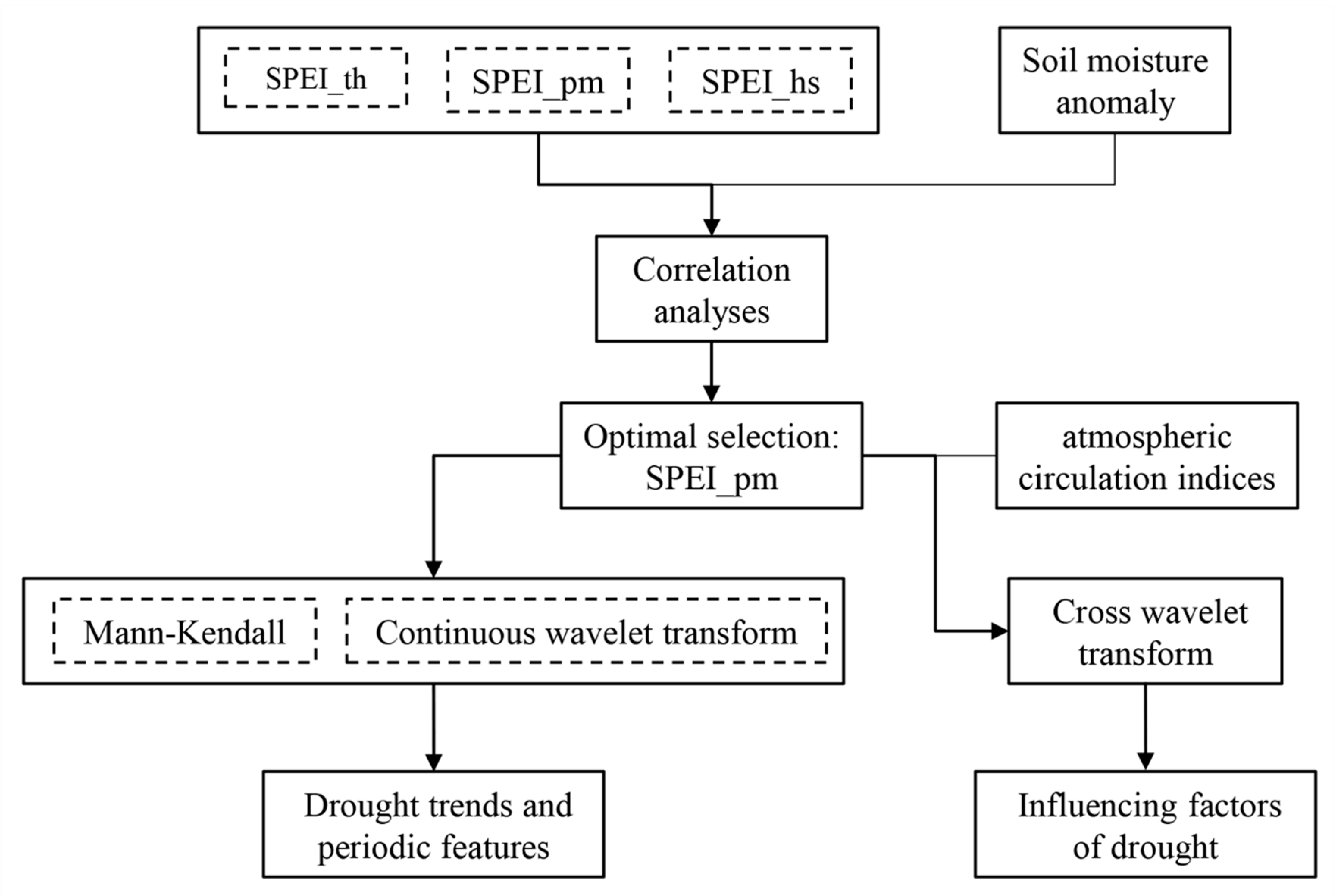
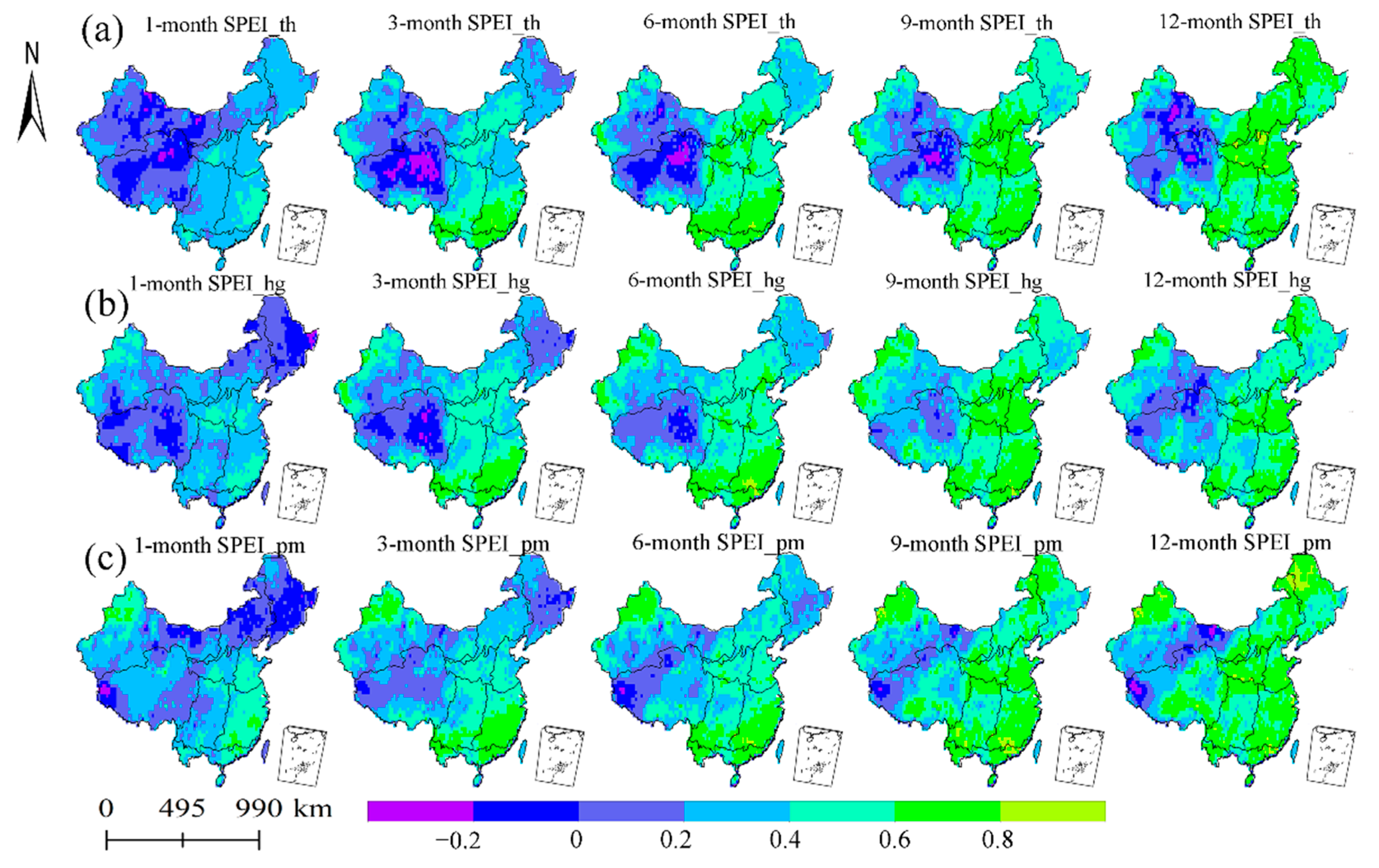
4.1. The Relation between SPEI and Soil Moisture Anomalies

Figure 3 displays the correlations between the SPEI, calculated using the TH, HS, and PM equations, and soil moisture anomalies at multiple time intervals (i.e., 1, 3, 6, 9, and 12 months) in China from 1961 to 2018. The correlations between the SPEI and soil moisture anomalies at different time intervals were obviously different. At a 1-month time interval, the correlation between SPEI and soil moisture anomalies was very weak, especially for SPEI_th in the GXR and QTR and SPEI_pm in the NECR; in all other regions, the correlations between the SPEI and soil moisture anomalies generally ranged between 0.2 and 0.6. The correlations at 3-month time intervals were, generally, slightly stronger than at 1-month intervals. For example, while the positive correlation between 3-month SPEI_th and soil moisture anomalies increased in the YRR and SCR, with r $\ge 0.6$, the negative correlation observed in the QTR decreased. There was a significant positive correlation between 3-month SPEI (calculated with TH and PM) and soil moisture anomalies in the YRR, SCR, and GXR. At a 6-month time interval, a significant positive correlation between SPEI_th and soil moisture anomalies was found in the HHHR and LPR, while the negative correlation in northeast QTR increased. The correlations at the 6-month interval between SPEI_hs and soil moisture anomalies were generally consistent with those at 3 months; however, the correlations between SPEI_pm and soil moisture anomalies at the 6-month interval exhibited an increase. At the 9-month interval, all correlations between the SPEI and soil moisture anomalies were significant, especially in the HHHR, MGR, LPR, YRR, and SCR. However, while SPEI_th showed an obvious negative correlation with soil moisture anomalies at the 9-month interval in northeast QTR, only weak negative correlations were detected with SPEI_hs and SPEI_pm. Furthermore, at the 9-month interval, the SPEI_pm also had a strong positive correlation with soil moisture anomalies in the NECR and GXR. For the 12-month interval, the correlation between SPEI and soil moisture anomalies was relatively strong across all agricultural regions, indicating that using a 12-month interval is best when relating the SPEI to soil moisture anomalies. Areas with correlation coefficients greater than 0.6 were more widely distributed when using a 12-month time interval, which meant that the positive correlation between the SPEI and soil moisture anomalies was strong for the Chinese mainland overall.

Soil moisture anomalies can directly reflect drought conditions, so if the SPEI is positively correlated with soil moisture anomalies at a given time interval, it means that the SPEI with the appropriate PET equation can accurately describe droughts. With the exception of the GXR and QTR, the correlation coefficients of the 12-month interval SPEI_th and SPEI_pm exceeded 0.6. In the cases of the GXR and QTR, negative correlation coefficients were found for the 12-month interval SPEI_th, indicating that the interval or calculation may not accurately capture the dry conditions in the GXR and QTR. The reason for the differences may be that the TH equation only considers temperature and ignores wind speed, radiation, and other factors. In arid regions (i.e., GXR and QTR), other climate factors (i.e., wind speed, relative humidity, and radiation) have a greater impact on PET and drought changes [26], so the SPEI based on the TH equation may not be able to reflect the changes in dryness and wetness. In contrast, at the 12-month interval, the SPEI_pm had no obvious negative correlations with soil moisture anomalies, and the positive correlation coefficients in the NECR exceeded 0.8, indicating that it more accurately reflected the drier agricultural regions of the Chinese mainland from 1961 to 2018.

These results showed that the PM equation provided better results for drought identification. A potential explanation may be that the PM method is based on physics; when data are sufficient, the PM method should be the better choice. The PM method has been adopted by the Food and Agriculture Organization of the United Nations (FAO) and the American Society of Civil Engineers (ASCE) as the standard procedure for computing PET. Precipitation, temperature, and PET are the three key variables of the SPEI because they strongly influence the occurrence of droughts. Therefore, the error and uncertainty of these three variables greatly affect the accuracy of the SPEI. Generally, precipitation and temperature can be assessed quantitatively using accurate measurements and can be used directly in the calculation of the SPEI. However, the calculation equation for PET remains controversial. Different equations for calculating PET include different climatic variables and emphasize different variables differently, resulting in inconsistent results. Despite this controversy, it is widely recognized that PET heavily influences soil moisture anomalies’ variability. Therefore, by choosing PM as the PET equation based on the correlation between soil moisture anomalies and the SPEI, the accuracy of this index in reflecting actual drought conditions is improved. Therefore, in this study, the SPEI calculated at a 12-month interval using the PM method was used to assess drought trends and the impacts of atmospheric circulation factors on drought throughout the Chinese mainland. However, the weak correlation between SPEI_pm and soil moisture anomalies in the GXR and QTR, even at the 12-month interval, indicates that this method may not accurately reflect drought conditions in these two areas. Though the 12-month scale SPEI can well characterize changes in soil moisture in humid areas, it may be not a good indicator of changes in soil moisture in complex arid areas. Since the soil moisture may be not closely related to climate change (e.g., precipitation) in arid areas, the change in soil moisture in arid areas thus has a weak relationship with meteorological drought [26].

4.2. Drought Trends and Periodic Features

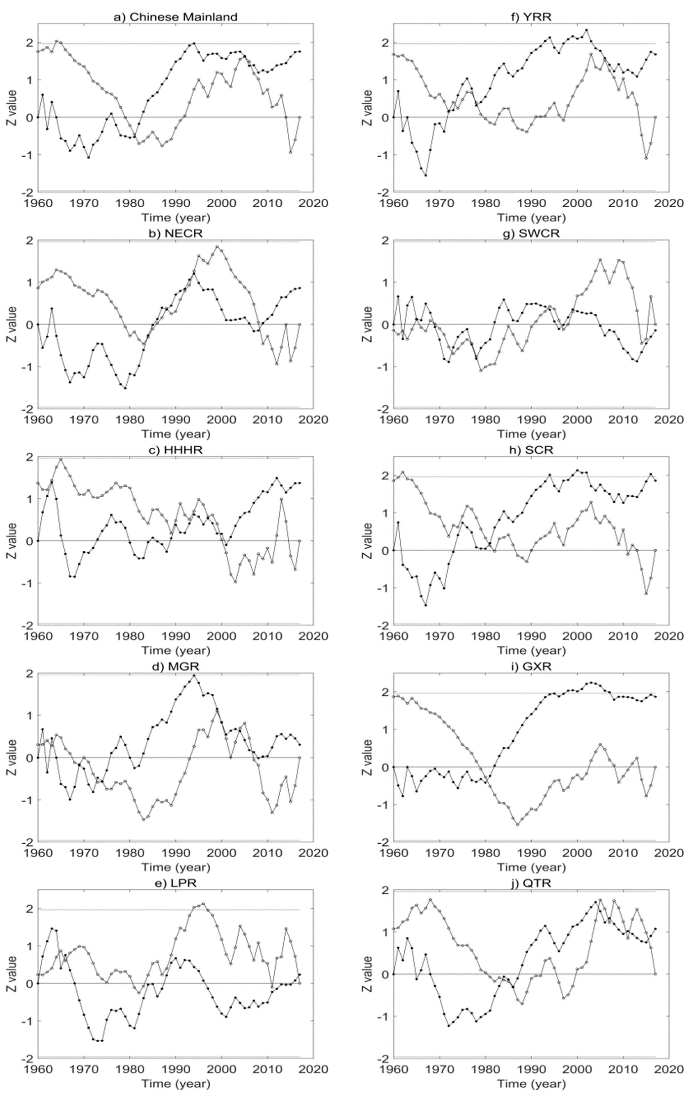
4.2.1. Drought Trends and Abrupt Change Analysis

The MK test was conducted to analyze the 12-month SPEI_pm series from the nine major agricultural areas and Chinese mainland, and the results are shown in Figure 4a–j and

Table 3. The annual drought trends (Z-value) in China and nine regions during 1961 to 2018.

NECR	HHHR	MGR	LPR	YRR	SWCR	SCR	GXR	QTR	Mainland
2.11	2.04	−0.47	0.21	2.15	−0.47	0.72	6.45	2.41	2.61

Note: The bold font indicates significant correlations.

. The UF and UB curves represent the forward and backward sequences. The Chinese mainland exhibited a significant wetting trend from 1961 to 2018. The UF and UB curves intersected between 1981 and 1982, at which time the UF and UB curves exceeded the critical value of ± 1.96, indicating that the sudden wet change was significant (Figure 4a). The NECR also had a significant wetting trend from 1961 to 2018. Figure 4b shows that the UF and UB curves of the NECR intersected at more than one time point, but neither of the wetting change points was significant. The HHHR showed a significant wetting trend during 1961–2018. The UF and UB curves intersected between 1999 and 2000, but the change point did not attain the 0.05 significance level (Figure 4c). The MGR displayed an insignificant drying trend from 1961 to 2018 and the UF and UB curves intersected at more than one time point, but none of the change points was significant (Figure 4d). An insignificant wetting trend appeared in LPR from 1961 to 2018. The UF and UB curves intersected at more than one time point, but the change points were insignificant (Figure 4e). There was a significant increasing trend in wetting in the YRR from 1961 to 2018. The UF and UB curves intersected at more than one time point, with a wet mutation point between 1971 and 1972 (Figure 4f). The UF and UB curve exceeded the critical value ± 1.96, which meant that the annual sudden wet change was significant. There was an insignificant drying trend observed in the SWCR from 1961 to 2018, and the change point did not reach the significance level of 0.05, which meant that the mutation was insignificant (Figure 4g). The SCR presented an insignificant wetting trend from 1961 to 2018. However, Figure 4h shows that the UF and UB curves intersected between 1980 and 1981, and they both exceeded the critical value ± 1.96, which means that this sudden change in wetting was significant. A significant wetting trend was apparent in the GXR from 1961 to 2018, with the UF and UB curves intersecting between 1980 and 1981 at a point above the critical value ± 1.96, indicating a significant wetting change (Figure 4i). The QTR also exhibited a significant wetting trend from 1961 to 2018, but the change point was insignificant (Figure 4j), implying that the abrupt change was also insignificant.

Overall, among the nine agricultural areas, the NECR, YRR, QTR, HHHR, and GXR had significant wetting trends, while the other four agricultural areas had an insignificant change. If viewed from the perspective of the entire Chinese mainland, the environment became significantly wetter. A study by Chen et al. [68] concluded that the SPEI revealed wetting trends at the national scale and that increases in wetness occurred in arid regions and the Qinghai-Tibet Plateau, while drying trends occurred in semi-arid, cold-semi-humid, and temperate-semi-humid regions. Furthermore, from the perspective of climatic regions, they found that drying trends tended to occur in transitional regions between the humid and arid regions of China, which was consistent with our results. In addition, Huang et al. [2] drew a similar conclusion when looking at drought structure in terms of duration, with the onset and termination of droughts in China remaining stable, with no noticeable change, except in the Pearl River basin (PRB) and the Haihe basin. According to the prediction by Wang et al. [69], in most areas of the PRB, especially the mid-west PRB, drought area is expected to expand in size and the drought severity and variability are projected to increase in the 21st century. However, other studies have suggested that East China will become drier due to the weakening of the summer monsoon caused by El Niño-like warming in the tropical Pacific [70].

The contributing factors to drying or wetting trends can be diverse; however, drought is most strongly related to precipitation, temperature, and PET. China has undergone a clear warming trend in recent decades, and it has been shown that the rising monthly temperature [71] enhances the significant upward trend in PET during most months. However, Piao et al. [72] found that, in spite of clear trends in climate (especially temperature), their overall impacts were obscured by natural variability and uncertainties in crop responses and projected climate, especially precipitation. A similar phenomenon may have occurred in this study, with the combined effects of various factors potentially obscuring any drying or wetting trends in the SCR, LPR, SWCR, or MGR, which did not show any significant trends. Based on the study by Foo Hui-Mean et al. [31], regions with increasing trends in PET should receive a higher level of attention with regard to drought potential, and regions with downward trends in PET may become wetter conversely. Importantly, a significant annual decreasing trend in PET occurred from 1961 to 2013 [73]. This was true for the Chinese mainland, NECR, YRR, QTR, HHHR, and GXR in this study, with downward trends in PET being related to the increase in moisture from 1961 to 2018.

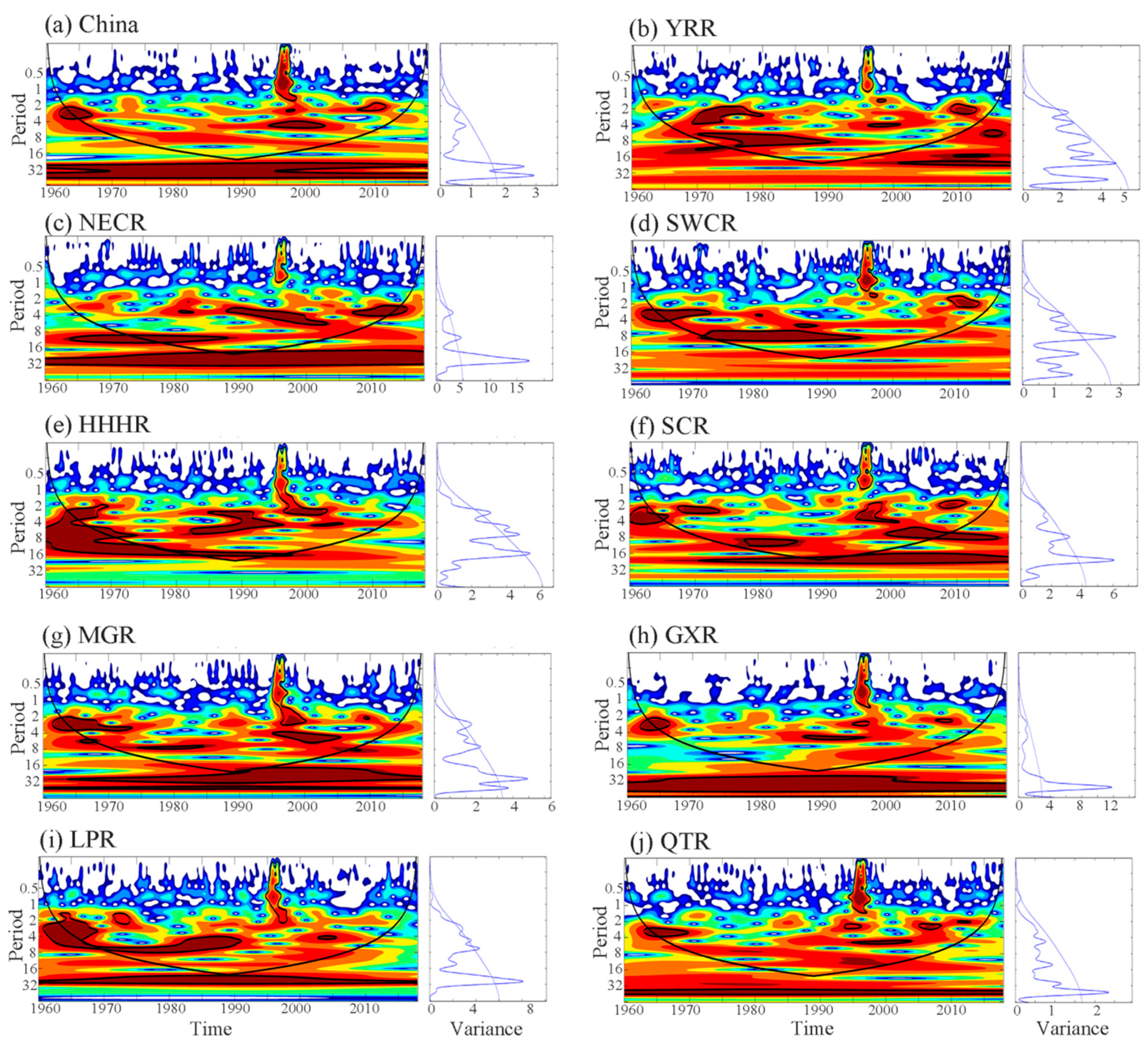
4.2.2. Periodic Oscillation

The results of CWT for the 12-month SPEI_pm series are shown in Figure 5. The 12-month SPEI_pm series showed that droughts in the Chinese mainland exhibited 2.8 and 4.6-year periods from 1961 to 2018 (Figure 5a). Inter-annual oscillations of 2–4 years were observed between 1963 and 1968 but only reached the 95% confidence level between 1966 and 1968. In addition, from 1995 to 2003, significant inter-annual oscillations were observed on a 4–6-year scale. The same CWT analysis was conducted to analyze the 12-month SPEI_pm series of the nine major agricultural areas; the results are shown in Figure 5b–j and

Table 4. Periodic oscillation of the nine agricultural regions and the entire China during 1961–2018.

Region	Period	Min Period	Inter-Annual Oscillations	Significant Period
NECR	3.3/11	3.3 11	2–4-year band 8–12-year band	2008–2016 1965–1988
HHHR	2.8/4.6/6.6	2.8 4.6 6.6	0–4-year band 2–8-year band 2–16-year band	1996–2004 1983–1996 1961–1998
MGR	2.8/4.6/6.6	2.8 6.6	2–4-year band 6–8-year band	1962–1974 1974–1985
LPR	2.8/4.6/6.6	2.8 4.6 6.6	1–8-year band 3–4-year band 4–8-year band	1962–1970 2002–2006 1970–1992
YRR	2.3/3.9/7.8	2.3	1–4-year band	1969–1980
SWCR	3.3/4.6/7.8	3.3 7.8	2–4-year band 6–10-year band	1962–1973 1970–1995
SCR	3.3/3.9/7.8	3.3 7.8	1–3-year band 4–8-year band	2008–2012 1999–2017
GXR	2.8/4.6	2.8	2–4-year band	1963–1968
QTR	3.3/4.6	-	-	-

. The results showed that droughts occurred mainly in 2.8, 3.3, 4.6, and 7.8-year periods in China, and the 2.8, 3.3, and 7.8-year periods were considered primary periods. Generally, a significant 2–8-year period of drought was detected in all nine major agricultural areas.

Recently, some studies have used CWT to analyze the periodic changes in drought in China. They found that the dominant significant oscillation periods were 2.5, 2.6, 4.4, 4.8, and 4.9 years [27,34]. For Southwest China, an annual SPEI_pm series analysis revealed 3.1-year and 8.7-year drought periods, but the 3.1-year period was dominant [19]. Furthermore, the significant wavelet power spectra for PET were found to have 2–6-year and 12–15-year periods [73,74], which were consistent with the significant periods returned when analyzing the SPEI, confirming the importance of PET in the SPEI. Although these studies used drought indices which were different from the index selected in this study, the drought periods were nearly identical.

4.3. Correlations with Large-Scale Atmospheric Circulation Indices

The Pearson correlation analyses were used to select the large-scale atmospheric circulation indices with the greatest impact on drought variation for the Chinese mainland and the agricultural regions. The correlation coefficients are shown in

Table 5. The correlation between the SPEI and atmosphere circulation.

Index	SCR	YRR	SWCR	LPR	QTR	HHHR	MGR	GXR	NECR	Mainland
WPTW	0.207	0.159	0.076	0.091	0.151	0.169	0.104	0.152	0.136	0.184
AAO	0.241	0.216	0.015	0.080	0.096	0.094	0.095	0.198	0.080	0.174
SCA	−0.146	−0.154	−0.051	−0.061	−0.103	−0.069	−0.069	−0.165	−0.081	−0.147
PSH	0.272	0.288	0.008	−0.042	0.004	0.047	−0.004	0.143	0.126	0.127
CPTW	0.010	−0.026	0.087	0.229	0.152	0.154	0.125	0.036	0.078	0.111
PSHA	0.259	0.276	−0.005	−0.053	−0.001	0.041	−0.003	0.146	0.129	0.122
WPSHI	0.292	0.310	−0.001	−0.081	−0.011	0.032	−0.014	0.138	0.120	0.119

Note: The bold font indicates significant correlations.

. The correlations that are greater than 0.273 are significant (p < 0.05). The results showed that, of all the atmospheric circulation indices, AAO, SCA, WPTW, PSH, CPTW, PSHA, and WPSHI had stronger correlations with the SPEI series of the nine major agricultural areas and Chinese mainland. The correlations between the SPEI and PSH, PSHA and WPSHI are significant (p < 0.05) in YRR, and the correlation between the SPEI of SCR and WPSHI is significant (p < 0.05). As for the other correlation coefficients in Table 5, they are insignificant. SPEI in humid areas (i.e., YRR) is often affected by precipitation, while PSH, PSHA, and WPSHI have a great influence on the precipitation process of YRR. For example, the WPSHI is a principal component of the East Asian summer monsoon system. The monsoon system brings a lot of precipitation, so the SPEI of YRR has a significant correlation with WPSHI [75]. The SCR is also a monsoon region, and its precipitation may be strongly affected by WPSHI, so its SPEI and WPSHI are significantly correlated. In terms of other indices, the atmospheric circulation may not be always the dominant condition for local drought, so the correlation is not always obvious.

Since the correlation between atmospheric circulation factors and SPEI is generally weak, the factors that have the greatest impact on each agricultural area should be studied separately. The circulation indices with the strongest influences on the SPEI were the WPTW for the Chinese mainland, NECR, and HHHR; CPTW for the MGR, LPR, and QTR; WPSHI for the YRR and SCR, and AAO for the GXR. All the above correlations between the SPEI series of agricultural regions and circulation indices were positive. The East Pacific subtropical ridge position index (EPSH) was the most influential circulation index for the SPEI of the SWCR and the correlation between them was negative. To further explore the driving forces behind drought evolution in the nine major agricultural regions of the Chinese mainland, cross-wavelet analysis was used to analyze the relationships between the SPEI and atmospheric circulation indices.

The results are shown in Figure 6. A common period was detected between the SPEI and WPTW in the 16–64-year scale from 1986 to 2009 in the Chinese mainland (Figure 6a). The WPTW had another period, mainly concentrated in the 16–32-year scale from 1978 to 1990, in common with the NECR (Figure 6b). The common period between the WPTW and the SPEI of the HHHR revealed a 24–32-year scale from 1999 to 2006 (Figure 6c), while the common period between the SPEI of the MGR and CPTW showed a 16–48-year scale from 1987 to 2001 (Figure 6d). Figure 6e shows that the common period between the SPEI of the LPR and CPTW was mainly concentrated in the 16–32-year scale from 1986 to 2002 and Figure 6f displays a common period of the same time scale from 1990 to 1999 between the SPEI of the YRR and WPSHI. In Figure 6g, it can be seen that the common period between the SPEI of the SWCR and EPSH was mainly concentrated in the 32–48-year scale from 2002 to 2011, and, as indicated by the left pointing arrow, they were negatively correlated, as was also indicated by the Pearson correlation coefficient. The common period between the SPEI of the SCR and WPSHI was in the 24–48-year scale from 1989 to 2002 (Figure 6h). In the case of the SPEI of the GXR and AAO, the common period was mainly observed in the 48–96-year scale from 1984 to 2005 (Figure 6i). Finally, the results showed that the common period between the SPEI of the QTR and CPTW was mainly concentrated in the 24–32-year scale from 1995 to 2000 (Figure 6j).

Atmospheric circulation exerted a strong effect on drought variation in China overall. However, each index measures different aspects of the atmospheric circulation and will therefore influence different areas differently. For example, the motion of the low atmosphere, as indicated by the WPTW and CPTW, could accelerate seawater evaporation, which would increase vapor at the ocean surface and grow into clouds, eventually leading to an increase in precipitation [76]. This may be the reason that the NECR, YRR, QTR, HHHR, GXR, and the Chinese mainland all showed a significant wetting trend. Previous studies have shown that the occurrence of dusty weather was strongly correlated with large-scale anomalous atmospheric circulation patterns, such as AAO [77], which agrees with the results of this study, where the SPEI and AAO were most significantly correlated in Northwest China, where dusty weather often occurs. The WPSHI and AAO both had a significant effect on the start, end, and duration of extreme precipitation periods over China, with each different region showing different effects [78]. A westward shift in the WPSHI, which enhances the East Asian early summer monsoon and consequently transports more moisture to Southern China, provides favorable moisture conditions for rainfall over the region [79]. One study, by Sun et al. [80], suggested that the AAO may impact the convective activity over the Maritime Continent, further strengthening the WPSHI and consequently resulting in anomalous rainfall over Southern China. Generally, an enhanced WPSHI can increase the southwesterly winds over Southern China and consequently advect more water vapor into the region, thereby favoring additional rainfall over Southern China. These findings showed that several circulation indices correlated well with the SPEI_pm series in this study and were likely the driving forces behind drought variation in China.

5. Conclusions

In this study, we chose the SPEI_pm method to describe drought variation and analyze influencing factors of drought in mainland China from 1961 to 2018. We conducted the MK test, correlation analysis, continuous wavelet analysis, and cross-wavelet analysis. The main conclusions of this study were as follows:

• Compared with the TH and HS methods, the PM method was most suitable for calculating PET. The correlation between the SPEI calculated using the PM equation and soil moisture anomalies was the strongest and was even stronger when a 12-month time interval was used.
• The NECR, YRR, QTR, HHHR, GXR, and Chinese mainland all showed significant wetting trends. Most of the abrupt changes in wetting occurred in the 1970s and 1980s, while in other agricultural areas, there was an insignificant change in their trends. The primary periods of the Chinese mainland were 2.3, 2.8, and 4.6-year periods and the primary periods of the nine major agricultural areas were 2.8, 3.3, and 7.8-year periods. A significant 2–4-year drought cycle period was detected in the Chinese mainland, while the lengths of the drought cycles in the nine major agricultural areas were generally distributed in the 2–8-year range.
• The AAO, SCA, WPTW, PSH, CPTW, PSHA, and WPSHI had the greatest impact on drought in China. In the NECR and HHHR, the WPTW index had the strongest positive correlation with the SPEI. In the MGR, LPR, and QTR, the CPTW index had the strongest positive correlations with the SPEI. In the YRR and SCR, the WPSHI index had the strongest positive correlation with the SPEI, and in GXR, the AAO index had the strongest positive correlations with the SPEI. Interestingly, the EPSH exhibited the dominant influence over the SPEI in the SWCR but had a negative correlation. In addition, a common period between the SPEI of the mainland of China and WPTW appeared in the 16–64-year scale from 1986 to 2009. For the nine major agricultural areas, however, the most significant common periods between their SPEI and their respective, most influential indices were in the 16–32-year scale.

References

1. Mishra, A.K.; Singh, V.P. A review of drought concepts. J. Hydrol. 2010, 391, 202–216. [Google Scholar] [CrossRef]
2. Huang, S.; Wang, L.; Wang, H.; Huang, Q.; Leng, G.; Fang, W.; Zhang, Y. Spatio-temporal characteristics of drought structure across china using an integrated drought index. Agric. Water Manag. 2019, 218, 182–192. [Google Scholar] [CrossRef]
3. Riebsame, W.E. Assessing the Social Implications of Climate Fluctuations: A Guide to Climate Impact Studies; World Climate Impacts Programme, United Nations Environment Programme: Boulder, CO, USA, 1988; pp. 75–82. [Google Scholar]
4. Xiao, M.; Zhang, Q.; Singh, V.P.; Liu, L. Transitional properties of droughts and related impacts of climate indices in the pearl river basin, china. J. Hydrol. 2016, 534, 397–406. [Google Scholar] [CrossRef] [Green Version]
5. Li, J.; Wang, Z.; Lai, C. Severe drought events inducing large decrease of net primary productivity in mainland china during 1982–2015. Sci. Total Environ. 2020, 703, 135541. [Google Scholar] [CrossRef]
6. Papadopoulou, M.P.C.D.; Spanoudaki, K.; Karali, A.; Varotsos, K.V.; Giannakopoulos, C.; Markou, M.; Loizidou, M. Agricultural water vulnerability under climate change in cyprus. Atmosphere 2020, 11, 648. [Google Scholar] [CrossRef]
7. Drysdale, R.E.; Bob, U.; Moshabela, M. Socio-economic determinants of increasing household food insecurity during and after a drought in the district of ilembe, south africa. Ecol. Food Nutr. 2020, 1–19. [Google Scholar] [CrossRef]
8. Hao, C.; Zhang, J.; Yao, F. Combination of multi-sensor remote sensing data for drought monitoring over southwest china. Int. J. Appl. Earth Obs. Geoinf. 2015, 35, 270–283. [Google Scholar] [CrossRef]
9. Lai, C.; Zhong, R.; Wang, Z.; Wu, X.; Chen, X.; Wang, P.; Lian, Y. Monitoring hydrological drought using long-term satellite-based precipitation data. Sci. Total Environ. 2019, 649, 1198–1208. [Google Scholar] [CrossRef]
10. McKee, T.; Doesken, N.; Kleist, J. The Relationship of Drought Frequency and Duration to Time Scales. In Proceedings of the 8th Conference on Applied Climatology, Anaheim, CA, USA, 17–22 January 1993; p. 17. [Google Scholar]
11. Li, J.; Wang, Z.L.; Wu, X.S.; Xu, C.Y.; Guo, S.L.; Chen, X.H. Toward monitoring short-term droughts using a novel daily scale, standardized antecedent precipitation evapotranspiration index. J. Hydrometeorol. 2020, 21, 891–908. [Google Scholar] [CrossRef]
12. Vicente-Serrano, S.; Beguería, S.; López-Moreno, J.I. A multiscalar drought index sensitive to global warming: The standardized precipitation evapotranspiration index. J. Clim. 2010, 23, 1696–1718. [Google Scholar] [CrossRef] [Green Version]
13. Jiao, W.; Tian, C.; Chang, Q.; Novick, K.A.; Wang, L. A new multi-sensor integrated index for drought monitoring. Agric. For. Meteorol. 2019, 268, 74–85. [Google Scholar] [CrossRef] [Green Version]
14. Zhong, R.; Chen, X.; Lai, C.; Wang, Z.; Lian, Y.; Yu, H.; Wu, X. Drought monitoring utility of satellite-based precipitation products across mainland china. J. Hydrol. 2019, 568, 343–359. [Google Scholar] [CrossRef]
15. Vicente-Serrano, S.M.; Van der Schrier, G.; Beguería, S.; Azorin-Molina, C.; Lopez-Moreno, J.-I. Contribution of precipitation and reference evapotranspiration to drought indices under different climates. J. Hydrol. 2015, 526, 42–54. [Google Scholar] [CrossRef] [Green Version]
16. Stagge, J.H.; Tallaksen, L.M.; Gudmundsson, L.; Van Loon, A.F.; Stahl, K. Candidate distributions for climatological drought indices (spi and spei). Int. J. Climatol. 2015, 35, 4027–4040. [Google Scholar] [CrossRef]
17. Beguería, S.; Vicente-Serrano, S.M.; Reig, F.; Latorre, B. Standardized precipitation evapotranspiration index (spei) revisited: Parameter fitting, evapotranspiration models, tools, datasets and drought monitoring. Int. J. Climatol. 2014, 34, 3001–3023. [Google Scholar] [CrossRef] [Green Version]
18. Yu, M.X.; Li, Q.F.; Hayes, M.J.; Svoboda, M.D.; Heim, R.R. Are droughts becoming more frequent or severe in china based on the standardized precipitation evapotranspiration index: 1951–2010? Int. J. Climatol. 2014, 34, 545–558. [Google Scholar] [CrossRef]
19. Wang, Z.; Huang, Z.; Zhong, R.; Zeng, Z.; Chen, X.; Li, J.; Lai, C. Increasing drought has been observed by spei_pm in southwest china during 1962–2012. Theor. Appl. Climatol. 2018, 133, 23–38. [Google Scholar] [CrossRef]
20. Cook, B.I.; Smerdon, J.E.; Seager, R.; Coats, S. Global warming and 21st century drying. Clim. Dyn. 2014, 43, 2607–2627. [Google Scholar] [CrossRef] [Green Version]
21. Unes, F.; Kaya, Y.Z.; Mamak, M. Daily reference evapotranspiration prediction based on climatic conditions applying different data mining techniques and empirical equations. Theor. Appl. Climatol. 2020, 141, 763–773. [Google Scholar] [CrossRef]
22. Yuan, S.; Quiring, S.M. Drought in the us great plains (1980–2012): A sensitivity study using different methods for estimating potential evapotranspiration in the palmer drought severity index. J. Geophys. Res. Atmos. 2014, 119, 10996–11010. [Google Scholar] [CrossRef]
23. Fang, W.; Huang, S.Z.; Huang, Q.; Huang, G.H.; Meng, E.H.; Luan, J.K. Reference evapotranspiration forecasting based on local meteorological and global climate information screened by partial mutual information. J. Hydrol. 2018, 561, 764–779. [Google Scholar] [CrossRef]
24. Van der Schrier, G.; Jones, P.D.; Briffa, K.R. The sensitivity of the pdsi to the thornthwaite and penman-monteith parameterizations for potential evapotranspiration. J. Geophys. Res. Atmos. 2011, 116, 116. [Google Scholar] [CrossRef]
25. Dai, A. Characteristics and trends in various forms of the palmer drought severity index during 1900–2008. J. Geophys. Res. Atmos. 2011, 116, 79–83. [Google Scholar] [CrossRef] [Green Version]
26. Sheffield, J.; Wood, E.F.; Roderick, M.L. Little change in global drought over the past 60 years. Nature 2012, 491, 435. [Google Scholar] [CrossRef]
27. Li, J.; Wang, Z.; Lai, C.; Zhang, Z. Tree-ring-width based streamflow reconstruction based on the random forest algorithm for the source region of the yangtze river, china. Catena 2019, 183, 104216. [Google Scholar] [CrossRef]
28. Zhang, B.; Wang, Z.; Chen, G. A sensitivity study of applying a two-source potential evapotranspiration model in the standardized precipitation evapotranspiration index for drought monitoring. Land Degrad. Dev. 2017, 28, 783–793. [Google Scholar] [CrossRef]
29. Allen, R.G.; Pereira, L.S.; Raes, D.; Smith, M. Crop Evapotranspiration: Guidelines for Computing Crop Requirements; FAO, Irrigation and Drainage: Roma, Italy, 1998; p. 56. [Google Scholar]
30. Hargreaves, G.H.; Allen, R.G. History and evaluation of hargreaves evapotranspiration equation. J. Irrig. Drain. Eng. 2003, 129, 53–63. [Google Scholar] [CrossRef]
31. Hui-Mean, F.; Yusop, Z.; Yusof, F. Drought analysis and water resource availability using standardised precipitation evapotranspiration index. Atmos. Res. 2018, 201, 102–115. [Google Scholar] [CrossRef]
32. Chen, H.P.; Sun, J.Q. Anthropogenic warming has caused hot droughts more frequently in china. J. Hydrol. 2017, 544, 306–318. [Google Scholar] [CrossRef]
33. Yang, J.; Gong, D.Y.; Wang, W.S.; Hu, M.; Mao, R. Extreme drought event of 2009/2010 over southwestern China. Meteorol. Atmos. Phys. 2012, 115, 173–184. [Google Scholar] [CrossRef]
34. Wang, Z.; Li, J.; Lai, C.; Zeng, Z.; Zhong, R.; Chen, X.; Zhou, X.; Wang, M. Does drought in china show a significant decreasing trend from 1961 to 2009? Sci. Total Environ. 2017, 579, 314–324. [Google Scholar] [CrossRef]
35. Ayantobo, O.O.; Li, Y.; Song, S.; Yao, N. Spatial comparability of drought characteristics and related return periods in mainland china over 1961–2013. J. Hydrol. 2017, 550, 549–567. [Google Scholar] [CrossRef]
36. Ionita, M.; Chelcea, S.; Rimbu, N.; Adler, M.J. Spatial and temporal variability of winter streamflow over romania and its relationship to large-scale atmospheric circulation. J. Hydrol. 2014, 519, 1339–1349. [Google Scholar] [CrossRef]
37. Li, J.; Wang, Z.; Wu, X.; Chen, J.; Guo, S. A new framework for tracking flash drought events in space and time. Catena 2020, 194, 104763. [Google Scholar] [CrossRef]
38. Liu, Z.; Zhou, P.; Zhang, F.; Liu, X.; Chen, G. Spatiotemporal characteristics of dryness/wetness conditions across qinghai province, northwest china. Agric. For. Meteorol 2013, 182–183, 101–108. [Google Scholar] [CrossRef]
39. Rubinetti, S.T.; Alessio, S.; Rubino, A.; Bizzarri, I.; Zanchettin, D. Robust decadal hydroclimate predictions for northern italy based on a twofold statistical approach. Atmosphere 2020, 11, 671. [Google Scholar] [CrossRef]
40. Wang, H.; Chen, Y.; Pan, Y.; Li, W. Spatial and temporal variability of drought in the arid region of china and its relationships to teleconnection indices. J. Hydrol. 2015, 523, 283–296. [Google Scholar] [CrossRef]
41. Wang, H.; Yang, Z.; Saito, Y.; Liu, J.P.; Sun, X. Interannual and seasonal variation of the huanghe (yellow river) water discharge over the past 50 years: Connections to impacts from enso events and dams. Glob. Planet. Chang. 2006, 50, 212–225. [Google Scholar] [CrossRef]
42. Zhang, Q.; Xu, C.Y.; Jiang, T.; Wu, Y. Possible influence of enso on annual maximum streamflow of the yangtze river, china. J. Hydrol. 2007, 333, 265–274. [Google Scholar] [CrossRef]
43. Yang, H.; Yang, D.; Hu, Q.; Lv, H. Spatial variability of the trends in climatic variables across china during 1961–2010. Theor. Appl. Climatol. 2015, 120, 773–783. [Google Scholar] [CrossRef]
44. Wu, Z.Y.; Lu, G.H.; Wen, L.; Lin, C.A. Reconstructing and analyzing china’s fifty-nine year (1951–2009) drought history using hydrological model simulation. Hydrol. Earth Syst. Sci. 2011, 15, 2881–2894. [Google Scholar] [CrossRef] [Green Version]
45. Zou, X.K.; Zhai, P.M.; Zhang, Q. Variations in droughts over china: 1951–2003. Geophys. Res. Lett. 2005, 32, 32. [Google Scholar] [CrossRef]
46. Xu, C.Y.; Gong, L.B.; Jiang, T.; Chen, D.L.; Singh, V.P. Analysis of spatial distribution and temporal trend of reference evapotranspiration and pan evaporation in changjiang (yangtze river) catchment. J. Hydrol. 2006, 327, 81–93. [Google Scholar] [CrossRef]
47. Xu, X.; Lin, H.; Hou, L.; Yao, X. An assessment for sustainable developing capability of integrated agricultural regionallization in china. Chin. Geogr. Sci. 2002, 12, 1–8. [Google Scholar] [CrossRef]
48. China Meteorological Administration. Available online: http://cdc.nmic.cn/home.do (accessed on 31 December 2018).
49. Community Land Model (CLM) of the Global Land Data Assimilation System (GLDAS). Available online: https://ldas.gsfc.nasa.gov/gldas) (accessed on 31 December 2018).
50. Rodell, M.; Houser, P.R.; Jambor, U.; Gottschalck, J.; Mitchell, K.; Meng, C.-J.; Arsenault, K.R.; Cosgrove, B.; Radakovich, J.; Bosilovich, M.; et al. The global land data assimilation system. Bull. Am. Meteorol. Soc. 2004, 85, 381. [Google Scholar] [CrossRef] [Green Version]
51. Zhang, J.Y.; Wang, W.C.; Wei, J.F. Assessing land-atmosphere coupling using soil moisture from the global land data assimilation system and observational precipitation. J. Geophys. Res. Atmos. 2008, 113, 14. [Google Scholar] [CrossRef]
52. Feng, X.; Fu, B.; Piao, S.; Wang, S.; Ciais, P.; Zeng, Z.; Lü, Y.; Zeng, Y.; Li, Y.; Jiang, X.; et al. Revegetation in china’s loess plateau is approaching sustainable water resource limits. Nat. Clim. Chang. 2016, 6, 1019. [Google Scholar] [CrossRef]
53. Climate Diagnostics and Prediction Division of the National Climate Center of China. Available online: https://cmdp.ncc-cma.net/cn/ (accessed on 31 December 2018).
54. Thornthwaite, C.W. An approach toward a rational classification of climate. Geogr. Rev. 1948, 38, 55–94. [Google Scholar] [CrossRef]
55. Hargreaves, G.L.; Samani, Z.A. Reference crop evapotranspiration from temperature. Appl. Eng. Agric. 1985, 1, 96–99. [Google Scholar] [CrossRef]
56. Guo, D.; Westra, S.; Maier, H.R. An r package for modelling actual, potential and reference evapotranspiration. Environ. Model. Softw. 2016, 78, 216–224. [Google Scholar] [CrossRef]
57. Torrence, C.; Compo, G.P. A practical guide to wavelet analysis. Bull. Am. Meteorol. Soc. 1998, 79, 61–78. [Google Scholar] [CrossRef] [Green Version]
58. Zhang, Q.; Xu, C.Y.; Zhang, Z.; Chen, Y.D.; Liu, C.L. Spatial and temporal variability of precipitation over china, 1951–2005. Theor. Appl. Climatol. 2009, 95, 53–68. [Google Scholar] [CrossRef]
59. Charlier, J.-B.; Ladouche, B.; Marechal, J.C. Identifying the impact of climate and anthropic pressures on karst aquifers using wavelet analysis. J. Hydrol. 2015, 523, 610–623. [Google Scholar] [CrossRef] [Green Version]
60. Gan, T.Y.; Gobena, A.K.; Wang, Q. Precipitation of southwestern canada: Wavelet, scaling, multifractal analysis, and teleconnection to climate anomalies. J. Geophys. Res. Atmos. 2007, 112, 112. [Google Scholar] [CrossRef]
61. Hao, Y.; Zhang, J.; Wang, J.; Li, R.; Hao, P.; Zhan, H. How does the anthropogenic activity affect the spring discharge? J. Hydrol. 2016, 540, 1053–1065. [Google Scholar] [CrossRef]
62. Grinsted, A.; Moore, J.C.; Jevrejeva, S. Application of the cross wavelet transform and wavelet coherence to geophysical time series. Nonlinear Processes Geophys. 2004, 11, 561–566. [Google Scholar] [CrossRef]
63. Nalley, D.; Adamowski, J.; Khalil, B.; Biswas, A. Inter-annual to inter-decadal streamflow variability in quebec and ontario in relation to dominant large-scale climate indices. J. Hydrol. 2016, 536, 426–446. [Google Scholar] [CrossRef]
64. Mann, H.B. Nonparametric tests against trend. Econometrica 1945, 13, 245–259. [Google Scholar] [CrossRef]
65. Kendall, M.G. Rank Correlation Methods; Griffin: London, UK, 1975. [Google Scholar]
66. Hamed, K.H.; Ramachandra Rao, A. A modified mann-kendall trend test for autocorrelated data. J. Hydrol. 1998, 204, 182–196. [Google Scholar] [CrossRef]
67. Yue, S.; Wang, C.Y. Applicability of prewhitening to eliminate the influence of serial correlation on the mann-kendall test. Water Resour. Res. 2002, 38, 1068. [Google Scholar] [CrossRef]
68. Chen, T.; Zhang, H.; Chen, X.; Hagan, D.F.T.; Wang, G.; Gao, Z.; Shi, T. Robust drying and wetting trends found in regions over china based on koppen climate classifications. J. Geophys. Res. Atmos. 2017, 122, 4228–4237. [Google Scholar] [CrossRef]
69. Wang, Z.; Zhong, R.; Lai, C.; Zeng, Z.; Lian, Y.; Bai, X. Climate change enhances the severity and variability of drought in the pearl river basin in south china in the 21st century. Agric. For. Meteorol. 2018, 249, 149–162. [Google Scholar] [CrossRef]
70. Dai, A. Drought under global warming: A review. Wiley Interdiscip. Rev. Clim. Chang. 2011, 2, 45–65. [Google Scholar] [CrossRef] [Green Version]
71. Suhaila, J.; Yusop, Z. Spatial and temporal variabilities of rainfall data using functional data analysis. Theor. Appl. Climatol. 2017, 129, 229–242. [Google Scholar] [CrossRef]
72. Piao, S.; Ciais, P.; Huang, Y.; Shen, Z.; Peng, S.; Li, J.; Zhou, L.; Liu, H.; Ma, Y.; Ding, Y.; et al. The impacts of climate change on water resources and agriculture in china. Nature 2010, 467, 43–51. [Google Scholar] [CrossRef]
73. Wang, Z.; Xie, P.; Lai, C.; Chen, X.; Wu, X.; Zeng, Z.; Li, L. Spatiotemporal variability of reference evapotranspiration and contributing climatic factors in china during 1961–2013. J. Hydrol. 2017, 544, 97–108. [Google Scholar] [CrossRef]
74. Zhang, K.-X.; Pan, S.-M.; Zhang, W.; Xu, Y.-H.; Cao, L.-G.; Hao, Y.-P.; Wang, Y. Influence of climate change on reference evapotranspiration and aridity index and their temporal-spatial variations in the yellow river basin, china, from 1961 to 2012. Quat. Int. 2015, 380–381, 75–82. [Google Scholar] [CrossRef]
75. Sun, J.; Huang, Y.M.; Han, J.; Zhang, X.P. Comparison on relationship between western pacific subtropical high and summer precipitation over dongting lake basin based on different datasets. Asia-Pac. J. Atmos. Sci 2020, 16. [Google Scholar] [CrossRef]
76. Ma, L.H.; Han, Y.B.; Yin, Z.Q. Quasi-biennial oscillation signals in outgoing long-wave radiation of the equator. Adv. Space Res. 2010, 46, 1477–1481. [Google Scholar] [CrossRef]
77. Fan, K.; Wang, H. Antarctic oscillation and the dust weather frequency in north china. Geophys. Res. Lett. 2004, 31, 31. [Google Scholar] [CrossRef] [Green Version]
78. Guo, X.; Wu, Z.-F.; He, H.S.; Du, H.; Wang, L.; Yang, Y.; Zhao, W. Variations in the start, end, and length of extreme precipitation period across china. Int. J. Climatol. 2018, 38, 2423–2434. [Google Scholar] [CrossRef]
79. Sun, J.; Ming, J.; Zhang, M.; Yu, S. Circulation features associated with the record-breaking rainfall over south china in June 2017. J. Clim. 2018, 31, 7209–7224. [Google Scholar] [CrossRef]
80. Sun, J.; Wang, H.; Yuan, W. A possible mechanism for the co-variability of the boreal spring antarctic oscillation and the yangtze river valley summer rainfall. Int. J. Climatol. 2009, 29, 1276–1284. [Google Scholar] [CrossRef]
Figure 1. Spatial distribution of Chinese agricultural regions and the 2417 meteorological stations. The different codes represent different regions: 1—Northeast China Region (NECR), 2—Huang-Huai-Hai Region (HHHR), 3—Inner Mongolia and the Great Wall Region (MGR), 4—Loess Plateau Region (LPR), 5—middle and lower regions of the Yangtze River (YRR), 6—Southwest China Region (SWCR), 7—South China Region (SCR), 8—Gan-Xin Region (GXR), 9—Qinghai-Tibet Plateau Region (QTR). The DEM in the figure represents the height above sea level in the digital elevation model.
Atmosphere 11 00990 g001
Figure 2. The flowchart of the methodology. Note: The SPEI_th, SPEI_hs, and SPEI_pm represent the PET of SPEI calculated by the TH, HS, and PM equations respectively.
Atmosphere 11 00990 g002
Figure 3. The correlation between monthly SPEI based on multiple PET equations ((a) TH, (b) HS, (c) PM) and soil moisture anomalies in China over the period of 1961–2018.
Atmosphere 11 00990 g003
Figure 4. Abrupt changes analysis for annual SPEI_pm of Chinese Mainland. (a) represents the Chinese mainland, and (bj) represent the NECR, HHHR, MGR, LPR, YRR, SWCR, SCR, GXR, and QTR, respectively. The solid points are on the UF curve and the hollow points are on the UB curve. UF and UB represent the statistics of forward and backward sequence, respectively.
Atmosphere 11 00990 g004
Figure 5. Wavelet analysis map of SPEI_pm in nine major Chinese agricultural regions. (a) represents the Chinese mainland. (bj) represent the YRR, NECR, SWCR, HHHR, SCR, MGR, GXR, LPR, and QTR, respectively. Figures on the left are wavelet power spectra; those on the right are the global wavelet power spectra. They are color-mapped to indicate high wavelet power with orange and low power in blue and white. The thick black contour in the left section designates the 95% confidence level against red noise, and the cone of influence (COI) where edge effects might distort the picture is shown in a lighter shade. The imaginary line in the right section designates the 95% confidence level for a red noise null hypothesis. If the peak of the solid line is above the imaginary line in the power map, then the corresponding period is significant.
Atmosphere 11 00990 g005
Figure 6. Cross-wavelet analysis for investigating the factors affecting SPEI variability: (a) SPEI and WPTW in Chinese mainland, (b) SPEI and WPSHI in YRR, (c) SPEI and WPTW in NECR, (d) SPEI and EPSH in SWCR, (e) SPEI and WPTW in HHHR, (f) SPEI and WPSHI in SCR, (g) SPEI and CPTW in MGR, (h) SPEI and AAO in GXR, (i) SPEI and CPTW inLPR, and (j) SPEI and CPTW in QTR. The thick black contour designates the 95% confidence level against red noise, and the cone of influence (COI) where edge effects might distort the picture is shown as a lighter shade. The cross-wavelet transform shows the relations between SPEI and WPTW/CPTW/WPSHI/EPSH/AAO. The relative phase relationship is shown as arrows (with in-phase pointing right, anti-phase pointing left).
Atmosphere 11 00990 g006