The Response of Parameterized Orographic Gravity Waves to Rapid Warming over the Tibetan Plateau

Abstract

Using the ERA-Interim reanalysis during 1979–2017, this work for the first time investigates the climatology and long-term trend of orographic gravity waves (OGWs) in the Tibetan Plateau (TP). The linkage between the trends of OGWs and the rapid warming over the TP is also studied. Climatologically, the most prominent surface wave momentum flux (SWMF) of OGWs occurs in the western and southeastern TP, while it is weak in the central TP. The SWMF is stronger in winter and spring than in autumn and summer. Overall, the mean SWMF over the TP experienced a weak decreasing trend. The decrease of SWMF mainly took place in the western and southeastern TP in spring. However, increasing trends were found in the central TP in winter. Changes of SWMF are mainly caused by the changes of horizontal wind near the surface, while buoyancy frequency and air density play a minor role. In response to the inhomogeneous warming over the TP, the surface winds were adjusted through thermal wind balance. In spring (winter), the most remarkable warming occurred in the northern (southern) TP, which reduced (enhanced) the meridional temperature gradient across the plateau, and thus led to a deceleration (acceleration) of the horizontal wind.

1. Introduction

The Tibetan Plateau (TP) includes the highest topography in the world, with a mean elevation over 4000 m. The TP and its surroundings are known as the third pole of the earth, because they have the largest number of glaciers outside the polar regions [1]. Due to the mechanical and thermal effects of its large-scale topography, the TP plays an important role in shaping the Asian climate patterns (e.g., the Asian Summer Monsoon) and even the global circulation [2].

In addition to the large-scale mountain ranges, there are also many smaller-scale terrain features over the TP, at horizontal lengths ranging from several kilometers to hundreds of kilometers (i.e., small-scale and mesoscale). Orographic gravity waves (OGWs) can be excited as stably stratified airflow goes over these mesoscale/small-scale mountains [3,4,5]. In fact, the TP is one of the hotspot regions for OGWs in the world, according to satellite observations, high-resolution numerical simulations and climate reanalysis [6,7,8,9] (see also Figure 1).

Although generated at the terrain surface, OGWs are capable of propagating upward to the middle atmosphere where the wave amplitude grows markedly owing to the decrease of air density with height [10]. Finally, OGWs break and deposit the wave momentum into the mean flow, exerting a synoptic-scale body force known as orographic gravity wave drag (OGWD) on the ambient wind. It has been found that OGWs play a key role in forcing the mesospheric circulation away from radiative equilibrium [11,12]. Additionally, the upper-level OGW forcing can affect the general circulation in the lower stratosphere and troposphere, through the so-called “downward control” mechanism [13]. Therefore, OGWs are of great importance in the coupling between the troposphere and middle atmosphere.

In recent years, there is an increasing concern about the dynamical impacts of OGWs that are generated over the TP. The parameterization of subgrid-scale orographic drag in the Weather Research and Forecasting (WRF) model can help alleviate the wind biases in the lower troposphere, which contributes to an improvement in the simulation of the regional wind circulation [14]. The low-level temperature and pressure fields are improved as well, in accordance with geostrophic balance. Based on the atmospheric and land components of the Community Earth System Model (CESM), Cohen and Boos investigated the response of wintertime precipitation to the forcing of orography in the TP region and surroundings [15]. Although the peak precipitation response to the OGWD due to mesoscale/small-scale orography only accounted for about one-third of that caused by stationary Rossby waves forced by large-scale orography, the OGWD response had a distinct structure and dominated in specific regions. From the point of view of “downward control”, in response to the localized OGWD forcing, the precipitation in the northwest (South) Asia was mainly suppressed (enhanced), resulting in a poleward shift of the intertropical convergence zone (ITCZ) over the near-equatorial Indo-West Pacific Ocean. Non-local effects of OGWs over the TP have also been found [16,17], using the Met Office Unified Model (MetUM) and the European Centre for Medium-Range Weather Forecasts (ECMWF) Integrated Forecasting System (IFS), and can affect the wind circulation and precipitation in the Northern Hemisphere at timescales ranging from days to seasons. For example, changes in the parameterized OGWs over the TP were found to be capable of influencing the wind circulation in the polar stratosphere by modifying the large-scale Rossby waves, because of the compensation between the forcing of OGWs and that of Rossby waves [18,19].

Past studies mainly focused on the weather and climate effects of OGWs using numerical modeling. However, the spatiotemporal characteristics of OGWs over the TP have rarely been addressed. Little is known about the climatology and especially the long-term trend of OGWs over the TP. The TP is one of the regions most sensitive to climate change [20]. Under the background effect of global warming during the second half of the 20th century, the TP experienced a persistent warming at a rate even faster than the average warming in the Northern Hemisphere [21,22]. There are many important consequences of TP warming. For instance, the area of glaciers over the TP shrank markedly, which affected the run-off of many prominent rivers in Asia [1,23]. The boreal spring sensible heat source over the TP, which had a great influence on the Asian summer monsoon [24], exhibited a decreasing trend, due largely to weakening of the surface wind [25,26]. From about 2000 onwards, however, the decreasing trend was replaced by a fast recovery, which was primarily caused by the increasing ground-air temperature difference [27]. Since OGWs owe their existence to the interaction between the land surface and the overlying atmosphere, changes in the atmospheric fields (e.g., temperature and wind) will also influence the generation of OGWs at the surface, and thus the OGW forcing aloft (i.e., OGWD). As studied in [28], the response of the wintertime circulation in the Northern Hemisphere to CO₂ doubling in a comprehensive atmospheric general circulation model is sensitive to the strength of the parameterized OGWD. Thus, understanding the changes of OGWs has wide implications for the simulation of the atmospheric general circulation and future projections of climate change.

In this work the spatiotemporal features of OGWs generated over the TP during 1979–2017 are investigated, which, to the authors’ knowledge, has not been done before. The main purpose is to understand the physical mechanisms that cause the long-term trend of OGWs under the rapid warming that has been occurring over the TP in recent decades. Changes in the vertical propagation of OGWs and the associated OGWD will be studied in a companion paper.

The rest of this paper is organized as follows. Section 2 describes the datasets and methods used. Section 3 firstly presents the 39-year climatology of OGWs over the TP. Then the long-term trends of OGWs in response to rapid warming over the TP are analyzed. Finally, the paper is summarized and discussed in Section 4.

2. Data and Methods

The intensity of gravity wave activity can be quantified by the momentum flux associated with these waves, i.e.,$\mathrm{F}=-\rho \overline{\mathrm{v}w}$, where $\rho$ is the air density, and v and $w$ are the horizontal and vertical velocity perturbations caused by gravity waves [29,30]. There have been a number of observational studies on the spatiotemporal features of gravity wave momentum fluxes at high altitudes, which were mainly derived from temperature fluctuations observed by satellite remote sensing [7,31,32]. However, there are no direct observations of OGWs generated at the terrain surface except very limited regional field experiments, e.g., the Mesoscale Alpine Program (MAP) [33]. To fill this gap, the 1° × 1°, daily momentum flux of OGWs from the ERA-Interim reanalysis is adopted, which is produced by cycle 31r2 of the ECMWF IFS model [34]. Benefiting from improved atmospheric model and assimilation system, ERA-Interim is a representative of third generation reanalysis. This dataset has been used in a number of studies including those over the TP [35,36,37,38], which thus confirmed the data quality.

Note that the OGWs excited by mesoscale/small-scale topography cannot be fully resolved by the IFS model given its relatively coarse horizontal resolution (~78 km). The surface wave momentum flux (SWMF) of OGWs is thus parameterized using the scheme developed by Lott and Miller [39] (1997, hereafter LM97), which is briefly described below.

In the LM97 scheme, the SWMF is assumed to be produced, within each model grid cell, by a horizontally elliptical bell-shaped mountain

$$h\left(x,y\right)=\frac{H}{1+{\left(x/a\right)}^2+{\left(y/b\right)}^2} ,$$

(1)

In the LM97 scheme, the SWMF is assumed to be produced, within each model grid cell, by a horizontally elliptical bell-shaped mountain where H is the mountain amplitude, and a and b are the half-widths in the cross-ridge and along-ridge directions, respectively. Parameters of the subgrid-scale orography (SSO) (e.g., standard deviation and anisotropy) are also available from the ERA-Interim reanalysis, and are derived from a realistic, high-resolution terrain elevation dataset. For example, Figure 2b shows the spatial distribution of the standard deviation of the SSO height over the TP, which is taken as a metric of the SSO amplitude, i.e., H in Equation (1). Large SSO standard deviations are mainly found along the periphery of the TP, especially in the western and southeastern TP. By contrast, the standard deviation of the SSO is rather small in the central TP. Based on linear gravity wave theory, the magnitude of the SWMF produced by an elliptical mountain is given by

$${\tau }_s=\rho NU{H}^{2}bG\sqrt{B^2{cos}^2\psi +C^2{sin}^2\psi },$$

(2)

where $N=\sqrt{\frac{g}{\theta }\frac{\partial \theta }{\partial z}}$ is the Brunt–Väisälä frequency, with $g$ being the gravitational acceleration and θ the potential temperature, U is the horizontal wind speed, ψ is the angle between the horizontal wind and the SSO ridge orientation, and G is a constant of order unity that depends on the shape of the orography. B and C are two constants determined by the SSO anisotropy (i.e., the horizontal aspect ratio $\mathsf{\gamma }=a/\mathrm{b}$), and are approximated as

$$B = 1–0.18\gamma –0.014{\gamma }^2, C = 0.48\gamma + 0.3{\gamma }^2.$$

(3)

Readers are referred to LM97 and references therein for more details about the parameterization scheme [39].

The daily SWMF is firstly averaged to obtain the monthly-mean and annual-mean SWMF. Then the long-term trend of the annual-mean SWMF over the TP (27° N–41° N, 70° E–105° E) is analyzed during the period of 1979–2017. Trends of SWMF in the four seasons, i.e., spring (March to May), summer (June to August), autumn (September to November), and winter (December to February), are examined as well. The statistical significance of the linearly-regressed trend is tested using the student-t test at a confidence level of 95%.

The warming trends over the TP are investigated using the 2-m temperature from ERA-Interim reanalysis. The reanalysis temperature is verified against daily surface temperature observations at 288 stations, most of which are located in the eastern part of the TP (see their geographical positions in Figure 2a). This observational dataset is provided by the National Meteorological Information Center of China Meteorological Administration (CMA), is subject to quality control and has been widely used for climate research in China [40,41,42].

3. Results

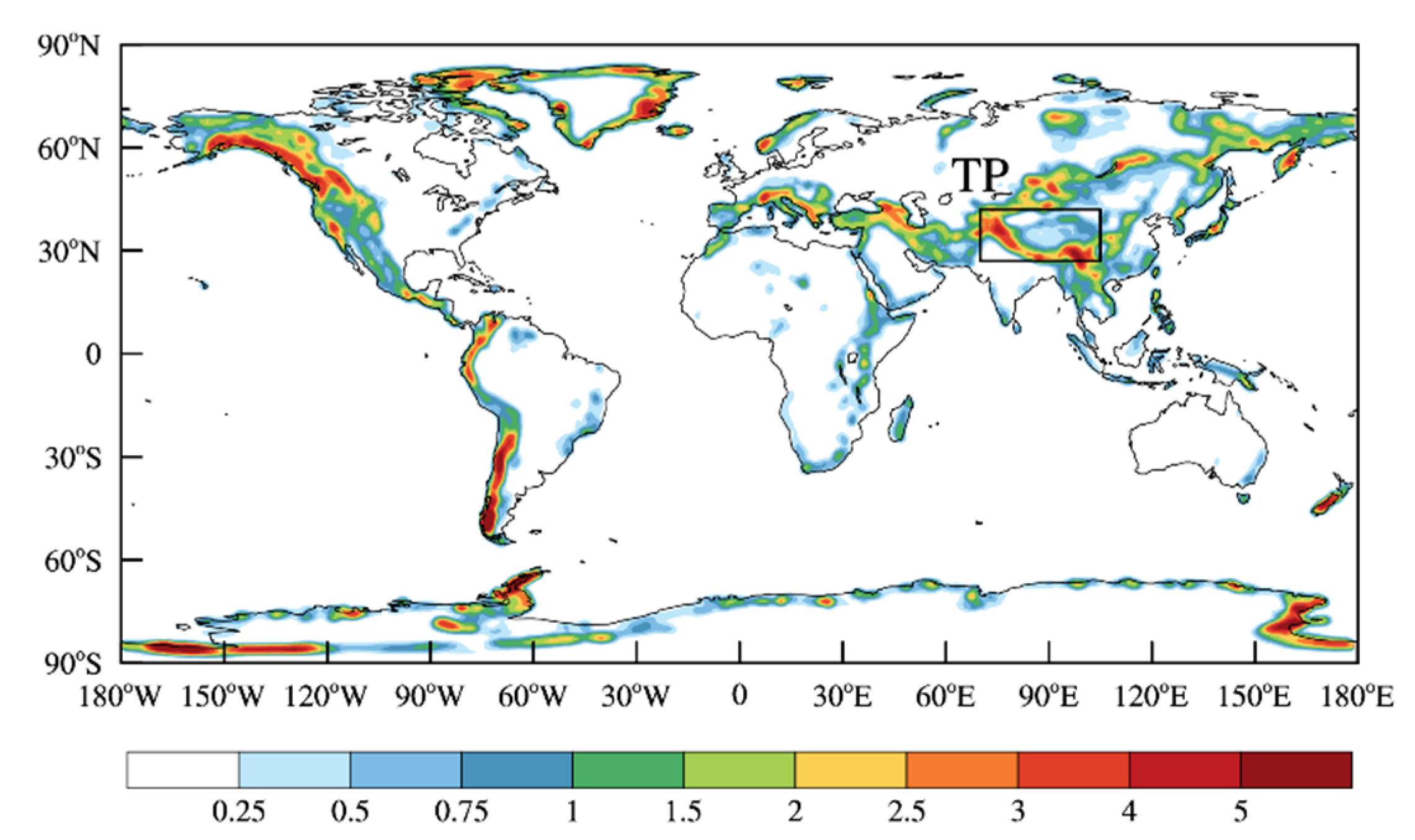
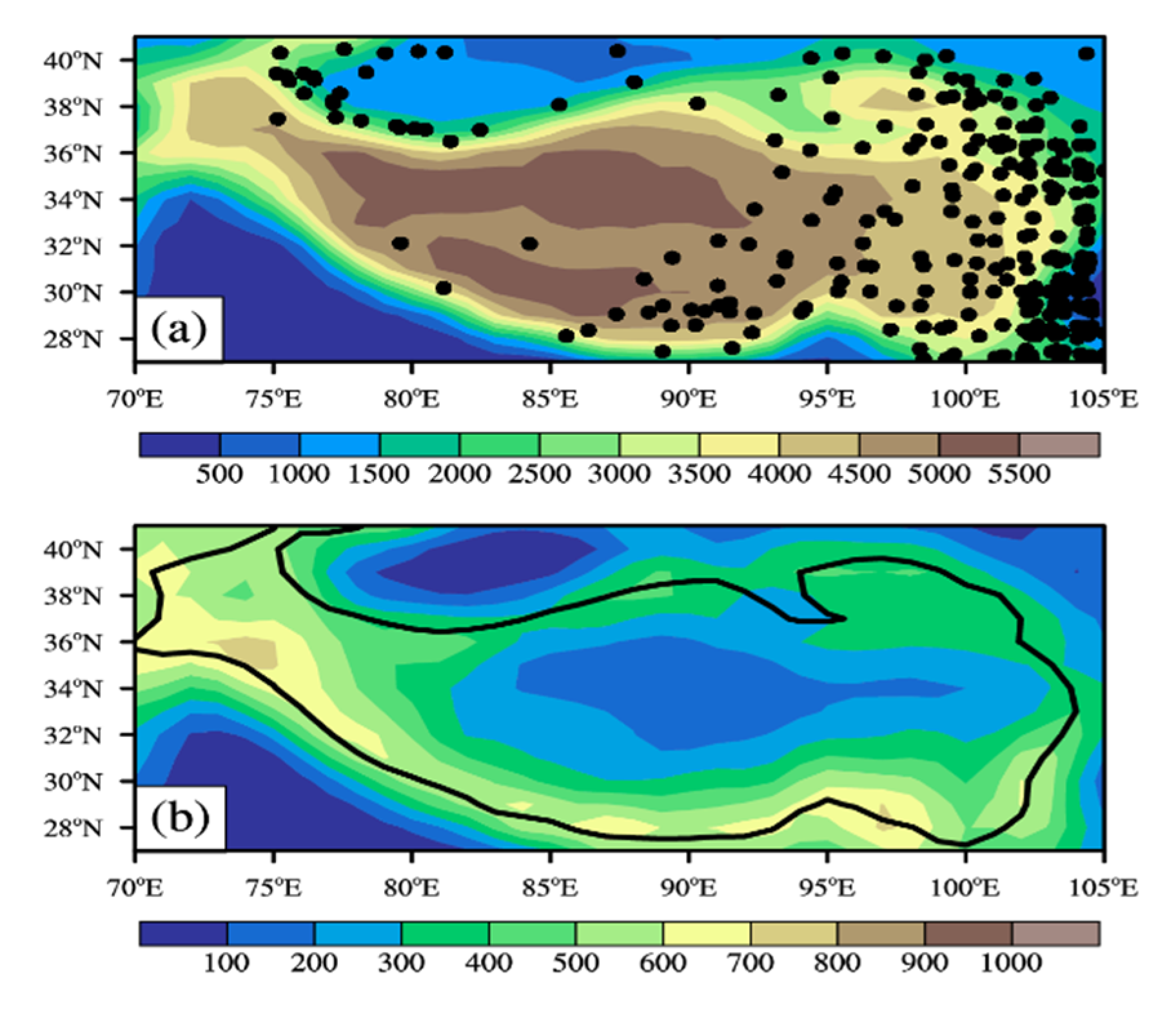
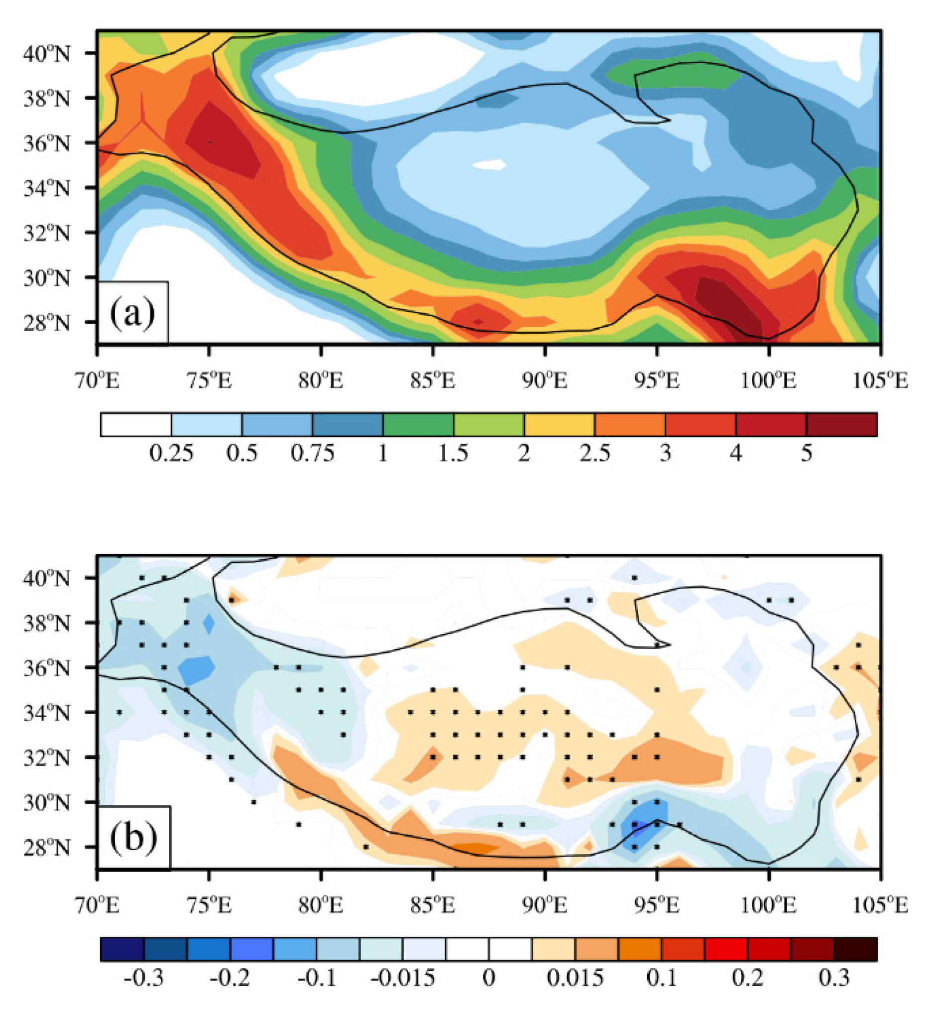
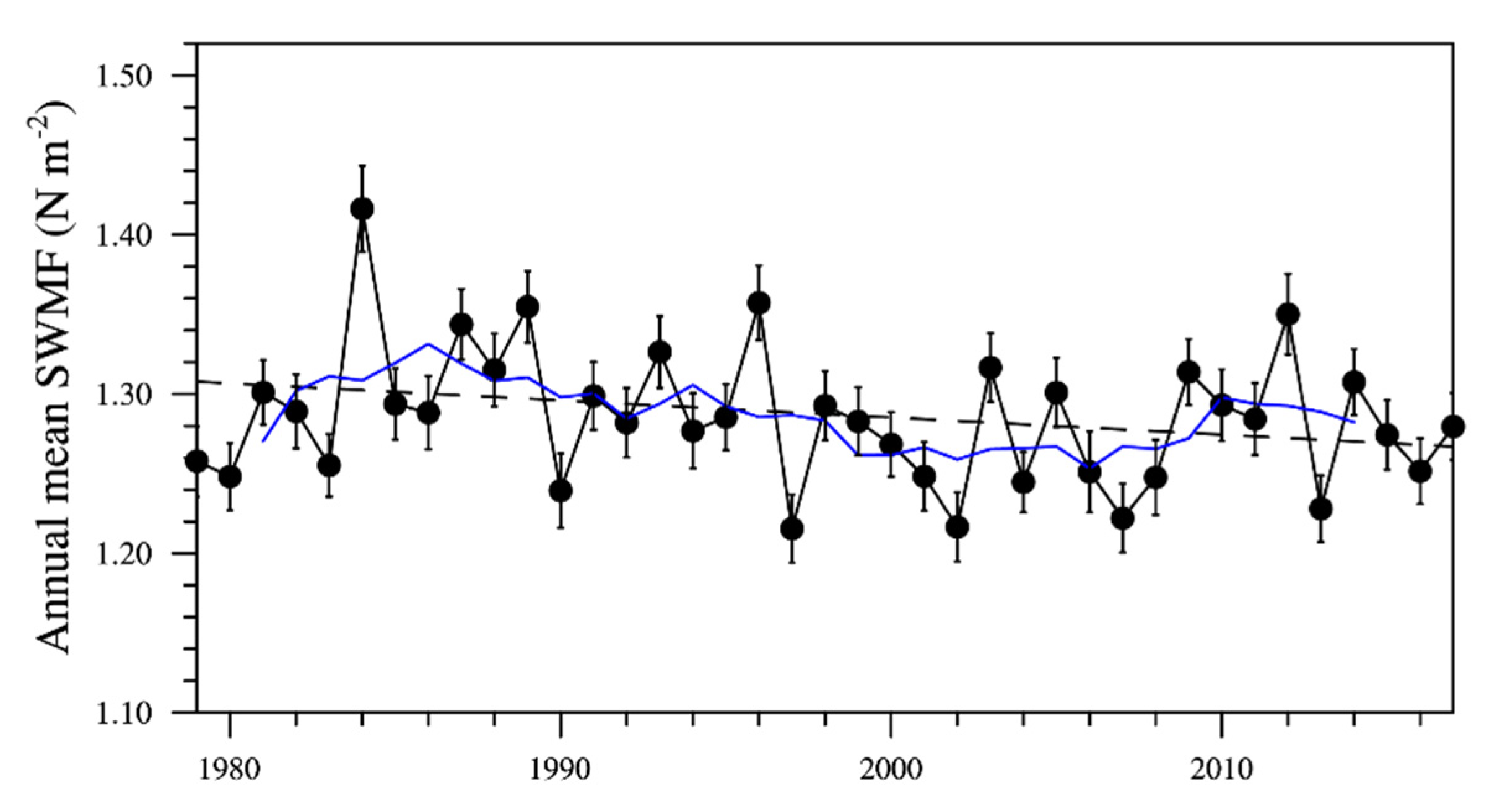
3.1. Climatology and Long-Term Trends of the SWMF

Figure 3a shows the spatial distribution of the SWMF over the TP averaged between 1979 and 2017. Climatologically, notable SWMFs are found in the western and southeastern TP, with maximum values exceeding 5 N m⁻². There also exists a relatively weak local maximum along the southern periphery of the TP, i.e., between the two maxima mentioned above. On the contrary, the SWMFs in the northern and central TP are much smaller, being as low as 0.5 N m⁻². Obviously, the spatial distribution of the SWMF is coherent with that of the SSO standard deviation (see Figure 2b).

In the four seasons of the year, the spatial patterns of the SWMF are quite similar to the annual pattern, with notable values found in the western and southern TP (not shown). However, the intensity of the SWMF exhibits a salient seasonal variation. SWMF is strongest in winter, with a mean value of 1.67 N m⁻² over the TP. There is also considerable SWMF in spring, which is 1.39 N m⁻² on average. On the contrary, the mean SWMF in summer is only 0.97 N m⁻² (accounting for about 58% of that in winter), which is the smallest value among the four seasons. The seasonal variation of the SWMF over the TP can be attributed to the seasonal cycle of horizontal winds, which are stronger in winter and spring than in autumn and summer (not shown).

Of greater interest is the long-term trend of the SWMF over the TP. In the past four decades, for the TP as a whole, the annual SWMF has decreased by about −7.9 × 10⁻³ N m⁻² decade⁻¹. However, this long-term trend is not statistically significant at 95% confidence level. As shown by the 5-year running average (blue line in Figure 4), the annual SWMF over the TP generally decreased roughly before the year 2000, while it started to increase afterwards. This change-point in the trend was further confirmed using the Mann–Kendall test method.

The long-term SWMF trends also exhibit considerable spatial variations over the TP. As shown in Figure 3b, the annual-mean SWMF was mainly reduced in 1979–2017 in the western and southeastern TP, at a rate of up to –0.15 N m⁻² decade⁻¹. On the contrary, there were weak but statistically significant increasing trends in the central TP, where the SWMF is climatologically small (see Figure 3a). The opposite SWMF trends found across the TP tend to cancel out each other, which may contribute to the insignificant long-term trend of the SWMF for the whole TP (Figure 3b).

Figure 5a–d is similar to Figure 3b but depicts the spatial distributions of SWMF trends in the four seasons, respectively. In spring (Figure 5a), significant decreasing trends were found in the western and southeastern TP, especially the former, which is of up to −0.3 N m⁻² decade⁻¹. In summer (Figure 5b), the SWMF experienced a decreasing trend in the western and southeastern TP as well, with the latter (former) being more (less) pronounced than its spring counterpart. By contrast, there were predominantly positive trends for the SWMFs in the northeastern, central, and southern TP. However, only the increases in the northeastern and in part of the central TP were statistically significant. In autumn (Figure 5c), the SWMF trends were basically weaker than in the other three seasons. Particularly, there was an increasing trend for the SWMF in the western TP, in contrast to that in spring and summer. In winter (Figure 5d), only the SWMFs in the central TP were significantly increased. Significant decreasing trends were found in part of the western and northeastern TP.

From the above analysis, the SWMFs were stronger in winter and spring than in summer and autumn, accompanied by faster trends. It can therefore be concluded that the increase of the SWMF in the central TP mainly took place in winter, while the decreasing trends found in the western and southeastern TP were largely due to the weakening of the SWMF in spring.

3.2. Cause of the SWMF Trends

From the point of view of fluid dynamics, OGWs are generated as stably stratified airflow goes over mountains and air parcels oscillate under the restoring force of buoyancy. In accordance with Equation (2), the magnitude of the SWMF is proportional to the air density, buoyancy frequency, and horizontal wind speed at the surface, depending as well on the geometric features of the SSO (e.g., height, half width and anisotropy). Given that the SSO is time-independent (at least at the timescale of tens of years considered in this study), changes in the SWMF should be caused by the time-varying atmospheric fields. In what follows, the long-term trends of the 10-m horizontal wind speed (SPD10), buoyancy frequency and air density at the surface are examined to help understand the changes of the SWMF over the TP.

Figure 6a presents the long-term trend of the annual-mean SPD10 over the TP, which is directly obtained from the ERA-Interim reanalysis. The geographical distribution of the SPD10 trend is very similar to that of SWMF (Figure 3b). A significant decrease of SPD10 was found in the western TP where the SWMF also notably decreased. Over the central TP, the SPD10 significantly increased by up to 0.1 m s⁻¹ decade⁻¹, which is consistent with the intensification of the SWMF there. In the southeastern TP, however, the SPD10 basically shows an increasing trend (except near 95° E) whereas the SWMF decreased. For the TP as a whole, the long-term trend of the domain-average SPD10 is not statistically significant, as shown in Figure 7a. This can be attributed to the spatial variability of the SPD10 trends across the TP, as was seen for the SWMF (Figure 3b). The 5-year running average of SPD10 (blue line in Figure 7a) is in very good agreement with that of the SWMF (see the blue line in Figure 4), which generally decreased roughly before 2000 but increased afterwards. The correlation coefficient (r) between these two time sequences is 0.67, well past the significance test at 95% confidence level.

The buoyancy frequency and air density at the surface are derived from the ERA-Interim reanalysis according to the definition $N=\sqrt{\frac{g}{\theta }\frac{\partial \theta }{\partial z}}$ and from the equation of state, respectively. Figure 6b illustrates the geographical distribution of the long-term trend of the annual-mean buoyancy frequency at the surface. Basically, there exist broad decline trends for the surface buoyancy frequency over the TP, in particular around 80° E. In the westernmost part of the TP, however, the surface buoyancy frequency increased, in contrast to the decrease of the SWMF observed there. In the central and southern TP, the long-term trends of the surface buoyancy frequency and of the SWMF are also out of phase, with an increase and a decrease, respectively. Overall, the domain-average surface buoyancy frequency over the TP significantly decreases, with a trend of −1.55 × 10⁻⁵ s⁻¹ decade⁻¹, during 1979–2017 (Figure 7b). The time sequence of the surface buoyancy frequency is negatively correlated to that of SWMF.

Similar to the buoyancy frequency at the surface, the air density predominantly decreased over the TP, with the most notable reduction occurring in the eastern part of the TP (Figure 6c). A weak increasing trend was found for the surface air density in a limited area over the western TP (between 70° E and 75° E), which opposes the decreasing trend of the SWMF there. On average, the annual-mean surface air density over the TP significantly decreased by about −4.21 × 10⁻⁴ kg m⁻³ decade⁻¹ (Figure 7c). Unlike the surface buoyancy frequency, the time sequence of the surface air density is positively correlated to that of SWMF. However, the correlation coefficient is too weak (r = 0.165) to pass the significance test. The pattern correlations between the trends of annual-mean SWMF and other parameters, including SPD10, buoyancy frequency and air density, are 0.10, −0.15, and −0.19, respectively, all of which are statistically significant at the 95% confidence level.

From the above analyses, changes of the annual-mean SWMF over the TP were primarily caused by those of the horizontal wind speed near the surface, whereas the buoyancy frequency and air density played a secondary role. The near-surface wind over the TP decreased roughly before 2000, consistent with the weakening of the East Asia monsoon [43]. Afterwards, there occurred a recovery of the near-surface wind, which was also found in [44]. The seasonal variations of the SWMF trends can also be explained by changes of the near-surface wind speed in the four seasons.

As mentioned in Section 3.1, the most prominent changes in the SWMF over the TP occurred in spring and winter. Figure 8a,b presents, respectively, the spatial patterns of the SPD10 trends in these two seasons. Generally, SPD10 in spring showed a decreasing trend over the TP (Figure 8a). In particular, this weakening is statistically significant in the western TP, where the SWMF also significantly decreased (Figure 5a). In the southwestern and southeastern TP, although SPD10 increased, in opposition to the decreasing trend of the SWMF there, its positive trend did not pass the significance test. In winter, SPD10 was overwhelmingly enhanced over the TP except in parts of the northeastern and western TP (Figure 8b). The most rapid increase occurred in the central TP, with an increasing trend of up to 0.1 m s⁻¹ decade⁻¹. This is consistent with the significant increase of the SWMF there (Figure 5d). In the southeastern and western TP, the long-term trends of SPD10 and SWMF also agree with each other. The long-term trends of the surface buoyancy frequency and air density in these two seasons were also analyzed (not shown). As happens with their annual trend, both the surface buoyancy frequency and air density increased in the western TP, in contrast with the decreasing trend of the SWMF there.

3.3. Linkage to TP Warming

In this section, we focus on the two seasons of spring and winter when the SWMF over the TP changed most markedly. Before exploring the relation between the changes of the SWMF and warming over the TP, Figure 9a,b firstly presents the long-term trends of the 2-m temperature from ERA-Interim reanalysis in spring and winter, respectively. In both seasons, a major part of the TP underwent a warming trend, most of which is statistically significant. In the western TP, there occurred a weak cooling trend for the 2-m temperature. In spring (Figure 9a), the 2-m temperature increased more rapidly in the northern than in the southern TP, with the maximum warming rate being of over 0.4 K decade⁻¹. Contrastingly, in the winter season (Figure 9b), the most prominent warming trends took place in the southern rather than in the northern TP.

The long-term trends of 2-m temperature from ERA-Interim reanalysis were verified against those of surface temperature from station observations, as shown in Figure 9c,d. Because of lack of meteorological stations in the western part of the TP (Figure 2a), only the temperature trends in the eastern TP were examined. In spring (Figure 9c), the warming rates were more notable in the northern than in the southern TP, and were generally faster than 0.4 K decade⁻¹. There were also warming trends along the northwestern periphery of the TP. Compared to those in spring, the warming trends in winter (Figure 9d) were generally stronger in the southern, southeastern, and central TP, but weaker in the northern TP. In particular, the most remarkable warming occurred in the central TP, exceeding 0.8 K decade⁻¹. Generally speaking, the long-term trends of the 2-m temperature from ERA-Interim reanalysis agree well with their observational counterparts in the eastern TP. Moreover, the seasonal variations of the inhomogeneous warming over the TP are also consistent with previous studies using the same station observations [40].

Because of warming at the surface, the static stability of the lower atmosphere is expected to be reduced. Buoyancy frequency ($N=\sqrt{\frac{g}{\theta }\frac{\partial \theta }{\partial z}}$) is proportional to the vertical gradient of potential temperature. Once warming at the surface, the vertical gradient of potential temperature will decrease, and thus the buoyancy frequency is reduced. This explains the widespread decreasing trends of surface buoyancy frequency over the TP (Figure 6b). The western TP, on the other hand, experienced a cooling trend (from reanalysis) such that the surface buoyancy frequency increased there. Air density trend is related to the temperature trend by the equation of state, which decreased (increased) with increasing (decreasing) temperature.

The relationship between the near-surface wind and temperature is not as straightforward as those between air density or buoyancy frequency and temperature. The large-scale wind in the free atmosphere is basically in geostrophic and thermal wind balance, i.e.,

$$V_{upper\_level}-V_{lower\_level}=\frac{R}{f}ln\frac{p_{lower\_level}}{p_{upper\_level}}k\times {\nabla }_p\overline{T}.$$

(4)

In spring, the warming trends in the northern TP were greater than in the western and southern TP, tending to weaken the meridional temperature gradient across the plateau. In consequence, the horizonal winds at upper levels, for example, 400 hPa, were reduced (Figure 10a). In winter, the most notable warming occurred in the southern TP, leading to an increase of the meridional temperature gradient and enhancement of the upper-level winds (Figure 10b).

Given the inhomogeneous warming at the surface, the difference between the horizontal winds in the upper level and surface will increase or decrease. In reality, the surface wind is very weak due to the presence of friction. Thus, changes in the vertical shear is mainly realized through the changes of upper-level winds (see Figure 10). Because of the elliptical nature of the quasi-geostrophic potential vorticity equation [45], the upper-level disturbances could have important consequences in the lower troposphere. This is confirmed by the high correlations between the 10-m and upper-level winds as noted below. For the TP as a whole, the correlation coefficients between the time series of 10-m and 400 hPa winds in spring and winter are 0.90 and 0.86, respectively, both of which well exceed the significance test at 95% confidence level. Even larger correlations were found with horizontal winds at lower levels, e.g., 500 hPa (Figure 10c,d), which are 0.92 and 0.87, respectively (

Table 1. Correlation coefficients between the time sequences of 10-m wind speed and upper-level wind speed in spring and winter during 1979–2017.

	500 hPa	400 hPa	300 hPa	200 hPa
Spring	0.92	0.90	0.81	0.76
Winter	0.87	0.86	0.78	0.72

Note: All the correlation coefficients are statistically significant at 95% confidence level using the student-t test.

), in spring and winter. This means that an increase (decrease) in meridional temperature gradient, which is correlated with an increase (decrease) in vertical wind shear (and consequently in the upper level winds), is in turn correlated with an increase (decrease) also in surface winds. Coherent trends of surface and upper-level winds in China had also been found in [44]. It has additionally been argued [46,47] that changes in the lower-tropospheric pressure-gradient force caused by inhomogeneous warming at the surface can to a large extent explain surface wind changes.

4. Summary and Conclusions

This work investigates for the first time the changes of orographic gravity waves (OGWs) over the Tibetan Plateau (TP) and explores their relationship with the rapid warming that has been occurring in recent decades in that region. Due to the lack of direct OGW observations at the surface, the surface wave momentum flux (SWMF) associated with OGWs available from ERA-Interim reanalysis is employed to represent the OGW activity. Being a subgrid-scale process, the SWMF is produced by the OGW parameterization scheme of the ECMWF Integrated Forecasting System (IFS) model, which was developed by Lott and Miller (1997, i.e., LM97) using mountain wave theory [39].

Based on the 1° × 1° daily SWMF data for the period 1979–2017, both the climatology and long-term trend of the SWMF over the TP were studied. The results showed that, climatologically, the strongest SWMF occurs in the western and southeastern TP, while the SWMF is rather weak in the central TP. In the four seasons, the SWMF possesses a spatial pattern similar to the annual one, but with a notable variation in intensity. Strong SWMFs were found in winter and spring, especially the former, while the SWMF is weakest in summer. In the period 1979–2017 the area-mean SWMF over the TP generally showed a decreasing trend, despite a recovery from about 2000 onwards. Further analysis revealed notable spatial and seasonal variations of the long-term trend of the SWMF. Decreases in SWMF mainly occurred in the western and southeastern TP in spring. By contrast, increasing trends were found over the central TP in winter.

According to the LM97 drag parameterization scheme, the parameterized SWMF increases as the horizontal wind, buoyancy frequency, and air density increase. To understand the changes of SWMF over the TP, the long-term trends of the horizontal wind speed, buoyancy frequency and air density at the surface were examined using ERA-Interim reanalysis. Results suggest that the changes in SWMF were mainly caused by those of the horizontal wind near the surface. For the TP as a whole, the time sequences of 10-m wind speed and SWMF during 1979–2017 are significantly correlated, with a high correlation coefficient of 0.67. The spatial and seasonal variations of the 10-m wind speed trend also agree well with those of the SWMF. The buoyancy frequency and air density at the surface, however, steadily decreased during 1979–2017, exhibiting no significant correlation with the SWMF. Moreover, inconsistencies were found between the spatial patterns of their long-term trends and that of the SWMF. While the SWMF significantly decreased in the western TP, the surface buoyancy frequency and air density increased there.

Changes in OGWs (in terms of their parameterized SWMF) in response to rapid warming over the TP can be understood by exploring the relationship between the horizontal wind and temperature at the surface. Using both ERA-Interim reanalysis and meteorological station observations, inhomogeneous warming patterns were found over the TP, with the horizontal wind adjusting according to thermal wind balance. In spring, there was greater warming in the northern than in the southern TP, which decreased the meridional temperature gradient across the TP, and thus decelerated the horizontal wind. The warming pattern was reversed in winter, with more notable warming in the southern TP. As a result, the horizontal winds were enhanced over the plateau.

This work provides some insight into the changes of land–atmosphere coupling over the TP from the perspective of OGWs, in the context of global warming. The present study focuses exclusively on the characteristics of OGWs at the surface (i.e., at the OGW source). Once generated, OGWs will propagate upward and affect the large-scale mean atmospheric circulation through transport of wave momentum [19]. In the context of climate change, will the propagation of parameterized OGWs also change in response to TP warming? Specifically, what will be the changes in the parameterized OGW momentum fluxes that enter the stratosphere from below? What are the consequences of these changing OGWs over the TP on the regional/global climate and weather? These issues will be addressed in future studies.

References

1. Yao, T.; Thompson, L.; Yang, W.; Yu, W.; Gao, Y.; Guo, X.; Yang, X.; Duan, K.; Zhao, H.; Xu, B.; et al. Different glacier status with atmospheric circulations in tibetan plateau and surroundings. Nat. Clim. Chang. 2012, 663–667. [Google Scholar] [CrossRef]
2. Wu, G.; Duan, A.; Liu, Y.; Mao, J.; Ren, R.; Bao, Q.; He, B.; Liu, B.; Hu, W. Tibetan plateau climate dynamics: Recent research progress and outlook. Natl. Sci. Rev. 2015, 100–116. [Google Scholar] [CrossRef] [Green Version]
3. Smith, R.B. The influence of mountains on the atmosphere. In Advances in Geophysics; Saltzman, B., Ed.; Elsevier: Amsterdam, The Netherlands, 1979; pp. 87–230. [Google Scholar]
4. Teixeira, M. The physics of orographic gravity wave drag. Front. Phys. 2014, 1–24. [Google Scholar] [CrossRef] [Green Version]
5. Xu, X.; Shu, S.; Wang, Y. Another look on the structure of mountain waves: A spectral perspective. Atmos. Res. 2017, 156–163. [Google Scholar] [CrossRef] [Green Version]
6. Cohen, N.Y.; Boos, W.R. Modulation of subtropical stratospheric gravity waves by equatorial rainfall. Geophys. Res. Lett. 2016, 466–471. [Google Scholar] [CrossRef] [Green Version]
7. Eckermann, S.; Preusse, P. Global measurements of stratospheric mountain waves from space. Science 1999, 1534–1537. [Google Scholar] [CrossRef] [Green Version]
8. Sato, K.; Watanabe, S.; Kawatani, Y.; Tomikawa, Y.; Miyazaki, K.; Takahashi, M. On the origins of mesospheric gravity waves. Geophys. Res. Lett. 2009. [Google Scholar] [CrossRef] [Green Version]
9. Xu, X.; Tang, Y.; Wang, Y.; Xue, M. Directional absorption of parameterized mountain waves and its influence on the wave momentum transport in the northern hemisphere. J. Geophys. Res. Atmos. 2018, 2640–2654. [Google Scholar] [CrossRef]
10. Lindzen, R. Turbulence and stress owing to gravity-wave and tidal breakdown. J. Geophys. Res. Oceans 1981, 9707–9714. [Google Scholar] [CrossRef] [Green Version]
11. Alexander, M.; Geller, M.; McLandress, C.; Polavarapu, S.; Preusse, P.; Sassi, F.; Sato, K.; Eckermann, S.; Ern, M.; Hertzog, A.; et al. Recent developments in gravity-wave effects in climate models and the global distribution of gravity-wave momentum flux from observations and models. Q. J. R. Meteorol. Soc. 2010, 1103–1124. [Google Scholar] [CrossRef]
12. Fritts, D.; Alexander, M. Gravity wave dynamics and effects in the middle atmosphere. Rev. Geophys. 2003. [Google Scholar] [CrossRef] [Green Version]
13. Haynes, P.; Marks, C.; Mcintyre, M.; Shepherd, T.; Shine, K. On the downward control of extratropical diabatic circulations by eddy-induced mean zonal forces. J. Atmos. Sci. 1991, 651–679. [Google Scholar] [CrossRef] [Green Version]
14. Zhou, X.; Yang, K.; Wang, Y. Implementation of a turbulent orographic form drag scheme in wrf and its application to the tibetan plateau. Clim. Dyn. 2017, 2443–2455. [Google Scholar] [CrossRef]
15. Cohen, N.Y.; Boos, W.R. The influence of orographic rossby and gravity waves on rainfall. Q. J. R. Meteorol. Soc. 2017, 845–851. [Google Scholar] [CrossRef] [Green Version]
16. Sandu, I.; Bechtold, P.; Beljaars, A.; Bozzo, A.; Pithan, F.; Shepherd, T.; Zadra, A. Impacts of parameterized orographic drag on the northern hemisphere winter circulation. J. Adv. Modeling Earth Syst. 2016, 196–211. [Google Scholar] [CrossRef] [Green Version]
17. van Niekerk, A.; Sandu, I.; Vosper, S. The circulation response to resolved versus parametrized orographic drag over complex mountain terrains. J. Adv. Modeling Earth Syst. 2018, 2527–2547. [Google Scholar] [CrossRef] [Green Version]
18. Cohen, N.; Gerber, E.; Buhler, O. Compensation between resolved and unresolved wave driving in the stratosphere: Implications for downward control. J. Atmos. Sci. 2013, 3780–3798. [Google Scholar] [CrossRef] [Green Version]
19. Xu, X.; Xue, M.; Teixeira, M.; Tang, J.; Wang, Y. Parameterization of directional absorption of orographic gravity waves and its impact on the atmospheric general circulation simulated by the weather research and forecasting model. J. Atmos. Sci. 2019, 3435–3453. [Google Scholar] [CrossRef]
20. Liu, X.; Chen, B. Climatic warming in the tibetan plateau during recent decades. Int. J. Climatol. 2000, 1729–1742. [Google Scholar] [CrossRef]
21. Liu, X.; Cheng, Z.; Yan, L.; Yin, Z. Elevation dependency of recent and future minimum surface air temperature trends in the tibetan plateau and its surroundings. Glob. Planet. Chang. 2009, 164–174. [Google Scholar] [CrossRef]
22. Zhong, L.; Su, Z.; Ma, Y.; Salama, M.; Sobrino, J. Accelerated changes of environmental conditions on the tibetan plateau caused by climate change. J. Clim. 2011, 6540–6550. [Google Scholar] [CrossRef]
23. Kang, S.C.; Zhang, Q.G.; Qian, Y.; Ji, Z.M.; Li, C.L.; Cong, Z.Y.; Zhang, Y.L.; Guo, J.M.; Du, W.T.; Huang, J.; et al. Linking atmospheric pollution to cryospheric change in the third pole region: Current progress and future prospects. Natl. Sci. Rev. 2019, 796–809. [Google Scholar] [CrossRef]
24. Wu, G.; Liu, Y.; He, B.; Bao, Q.; Duan, A.; Jin, F. Thermal controls on the asian summer monsoon. Sci. Rep. 2012. [Google Scholar] [CrossRef] [PubMed] [Green Version]
25. Duan, A.; Wu, G. Weakening trend in the atmospheric heat source over the tibetan plateau during recent decades. Part i: Observations. J. Clim. 2008, 3149–3164. [Google Scholar] [CrossRef] [Green Version]
26. Yang, K.; Guo, X.; He, J.; Qin, J.; Koike, T. On the climatology and trend of the atmospheric heat source over the tibetan plateau: An experiments-supported revisit. J. Clim. 2011, 1525–1541. [Google Scholar] [CrossRef]
27. Wang, M.; Wang, J.; Chen, D.; Duan, A.; Liu, Y.; Zhou, S.; Guo, D.; Wang, H.; Ju, W. Recent recovery of the boreal spring sensible heating over the tibetan plateau will continue in cmip6 future projections. Environ. Res. Lett. 2019. [Google Scholar] [CrossRef] [Green Version]
28. Sigmond, M.; Scinocca, J.; Kushner, P. Impact of the stratosphere on tropospheric climate change. Geophys. Res. Lett. 2008. [Google Scholar] [CrossRef]
29. Teixeira, M.; Yu, C. The gravity wave momentum flux in hydrostatic flow with directional shear over elliptical mountains. Eur. J. Mech. B Fluids 2014, 16–31. [Google Scholar] [CrossRef]
30. Xu, X.; Wang, Y.; Xue, M. Momentum flux and flux divergence of gravity waves in directional shear flows over three-dimensional mountains. J. Atmos. Sci. 2012, 3733–3744. [Google Scholar] [CrossRef] [Green Version]
31. Alexander, M.; Gille, J.; Cavanaugh, C.; Coffey, M.; Craig, C.; Eden, T.; Francis, G.; Halvorson, C.; Hannigan, J.; Khosravi, R.; et al. Global estimates of gravity wave momentum flux from high resolution dynamics limb sounder observations. J. Geophys. Res. Atmos. 2008. [Google Scholar] [CrossRef] [Green Version]
32. Ern, M. Absolute values of gravity wave momentum flux derived from satellite data. J. Geophys. Res. 2004. [Google Scholar] [CrossRef] [Green Version]
33. Bougeault, P.; Binder, P.; Buzzi, A.; Dirks, R.; Houze, R.; Kuettner, J.; Smith, R.; Steinacker, R.; Volkert, H. The map special observing period. Bull. Am. Meteorol. Soc. 2001, 433–462. [Google Scholar] [CrossRef] [Green Version]
34. Dee, D.; Uppala, S.; Simmons, A.; Berrisford, P.; Poli, P.; Kobayashi, S.; Andrae, U.; Balmaseda, M.; Balsamo, G.; Bauer, P.; et al. The era-interim reanalysis: Configuration and performance of the data assimilation system. Q. J. R. Meteorol. Soc. 2011, 553–597. [Google Scholar] [CrossRef]
35. Ji, Z.; Kang, S.; Cong, Z.; Zhang, Q.; Yao, T. Simulation of carbonaceous aerosols over the third pole and adjacent regions: Distribution, transportation, deposition, and climatic effects. Clim. Dyn. 2015, 2831–2846. [Google Scholar] [CrossRef]
36. Maussion, F.; Scherer, D.; Molg, T.; Collier, E.; Curio, J.; Finkelnburg, R. Precipitation seasonality and variability over the tibetan plateau as resolved by the high asia reanalysis. J. Clim. 2014, 1910–1927. [Google Scholar] [CrossRef] [Green Version]
37. Vellore, R.; Kaplan, M.; Krishnan, R.; Lewis, J.; Sabade, S.; Deshpande, N.; Singh, B.; Madhura, R.; Rao, M. Monsoon-extratropical circulation interactions in himalayan extreme rainfall. Clim. Dyn. 2016, 3517–3546. [Google Scholar] [CrossRef]
38. Yang, W.; Guo, X.; Yao, T.; Zhu, M.; Wang, Y. Recent accelerating mass loss of southeast tibetan glaciers and the relationship with changes in macroscale atmospheric circulations. Clim. Dyn. 2016, 805–815. [Google Scholar] [CrossRef]
39. Lott, F.; Miller, M. A new subgrid-scale orographic drag parametrization: Its formulation and testing. Q. J. R. Meteorol. Soc. 1997, 101–127. [Google Scholar] [CrossRef]
40. Duan, J.; Li, L.; Fang, Y. Seasonal spatial heterogeneity of warming rates on the tibetan plateau over the past 30 years. Sci. Rep. 2015. [Google Scholar] [CrossRef] [Green Version]
41. Tang, J.; Wang, S.; Niu, X.; Hui, P.; Zong, P.; Wang, X. Impact of spectral nudging on regional climate simulation over cordex east asia using wrf. Clim. Dyn. 2017, 2339–2357. [Google Scholar] [CrossRef]
42. Wang, P.; Tang, J.; Sun, X.; Liu, J.; Juan, F. Spatiotemporal characteristics of heat waves over china in regional climate simulations within the cordex-ea project. Clim. Dyn. 2019, 799–818. [Google Scholar] [CrossRef]
43. Xu, M.; Chang, C.; Fu, C.; Qi, Y.; Robock, A.; Robinson, D.; Zhang, H. Steady decline of east asian monsoon winds, 1969-2000: Evidence from direct ground measurements of wind speed. J. Geophys. Res. Atmos. 2006. [Google Scholar] [CrossRef] [Green Version]
44. Lin, C.; Yang, K.; Qin, J.; Fu, R. Observed coherent trends of surface and upper-air wind speed over china since 1960. J. Clim. 2013, 2891–2903. [Google Scholar] [CrossRef] [Green Version]
45. Holton, J.R. An Introduction to Dynamic Meteorology; Elsevier Academic Press: London, UK, 2004; p. 535. [Google Scholar]
46. Guo, H.; Xu, M.; Hu, Q. Changes in near-surface wind speed in china: 1969–2005. Int. J. Climatol. 2011, 349–358. [Google Scholar] [CrossRef]
47. You, Q.; Fraedrich, K.; Min, J.; Kang, S.; Zhu, X.; Pepin, N.; Zhang, L. Observed surface wind speed in the tibetan plateau since 1980 and its physical causes. Int. J. Climatol. 2014, 1873–1882. [Google Scholar] [CrossRef]
Figure 1. Global climatology of the surface wave momentum flux (SWMF) (units: N m−2) during 1979–2017 from the ERA-Interim reanalysis. The Tibetan Plateau (TP) is indicated by the black rectangular box.
Atmosphere 11 01016 g001
Figure 2. (a) Elevation (shading) (units: m) of the TP and locations of 288 weather stations (black dots). (b) Standard deviation of the subgrid orography. The black contour in (b) denotes the isoline of 3000-m elevation.
Atmosphere 11 01016 g002
Figure 3. (a) Climatology (units: N m−2) and (b) trend (units: N m−2 decade−1) of the SWMF over the TP during 1979–2017. The black contour denotes the isoline of 3000-m elevation. The dots in (b) indicate significant trends at 95% confidence level using the student-t test.
Atmosphere 11 01016 g003
Figure 4. Time series of the annual-mean SWMF (units: N m−2) over the TP during 1979–2017. Error bars represent standard errors. The blue line denotes the 5-yr running average, while the black dashed line is the linear trend during 1979–2017.
Atmosphere 11 01016 g004
Figure 5. Trends (units: N m−2 decade−1) of the SWMF over the TP during 1979–2017 in different seasons (a) spring (March–May), (b) summer (June–August), (c) autumn (September–November), and (d) winter (December–February). The black contour denotes the isoline of 3000-m elevation. The dots indicate significant trends at 95% confidence level using the student-t test.
Atmosphere 11 01016 g005
Figure 6. Annual trends of the (a) 10-m wind speed (units: m s−1 decade−1), (b) buoyancy frequency (units: 10−4 s−1 decade−1) and (c) air density (units: kg m−3 decade−1) at the surface over the TP during 1979–2017. The black contour denotes the isoline of 3000-m elevation. The dots indicate significant trends at 95% confidence level using the student-t test.
Atmosphere 11 01016 g006
Figure 7. Time series of annual mean (a) 10-m wind speed, (b) buoyancy frequency and (c) air density at the surface over the TP during 1979–2017. Error bars represent standard errors. Blue lines are the 5-yr running average. Black dashed lines in (ac) are the linear trends during 1979–2017.
Atmosphere 11 01016 g007
Figure 8. Trends (units: m s−1 decade−1) of the 10-m horizontal wind over the TP during 1979–2017 in different seasons (a) spring (March–May), (b) winter (December–February). The black contour denotes the isoline of 3000-m elevation. The dots indicate significant trends at 95% confidence level using the student-t test.
Atmosphere 11 01016 g008
Figure 9. Trends of the 2-m temperature (top, units: K decade−1) from the ERA-Interim reanalysis and surface temperature from observational stations (bottom, units: K decade−1) over the TP during 1979–2017. (a,c) are in spring (March–May), while (b,d) are in winter (December–February). The black contour denotes the isoline of 3000-m elevation. The dots in (a,b) and filled circles in (c,d) indicate significant trends at 95% confidence level using the student-t test.
Atmosphere 11 01016 g009
Figure 10. Trends of the 400 hPa (top) and 500 hPa (bottom) wind speed (units: m s−1 decade−1) over the TP during 1979–2017. (a,c) are in spring (March–May), while (b,d) are in winter (December–February). The black contour denotes the isoline of 3000-m elevation. The dots indicate significant trends at 95% confidence level using the student-t test.
Atmosphere 11 01016 g010