Traffic-Related Airborne VOC Profiles Variation on Road Sites and Residential Area within a Microscale in Urban Area in Southern Taiwan

Abstract
:1. Introduction
2. Experimental Methodology
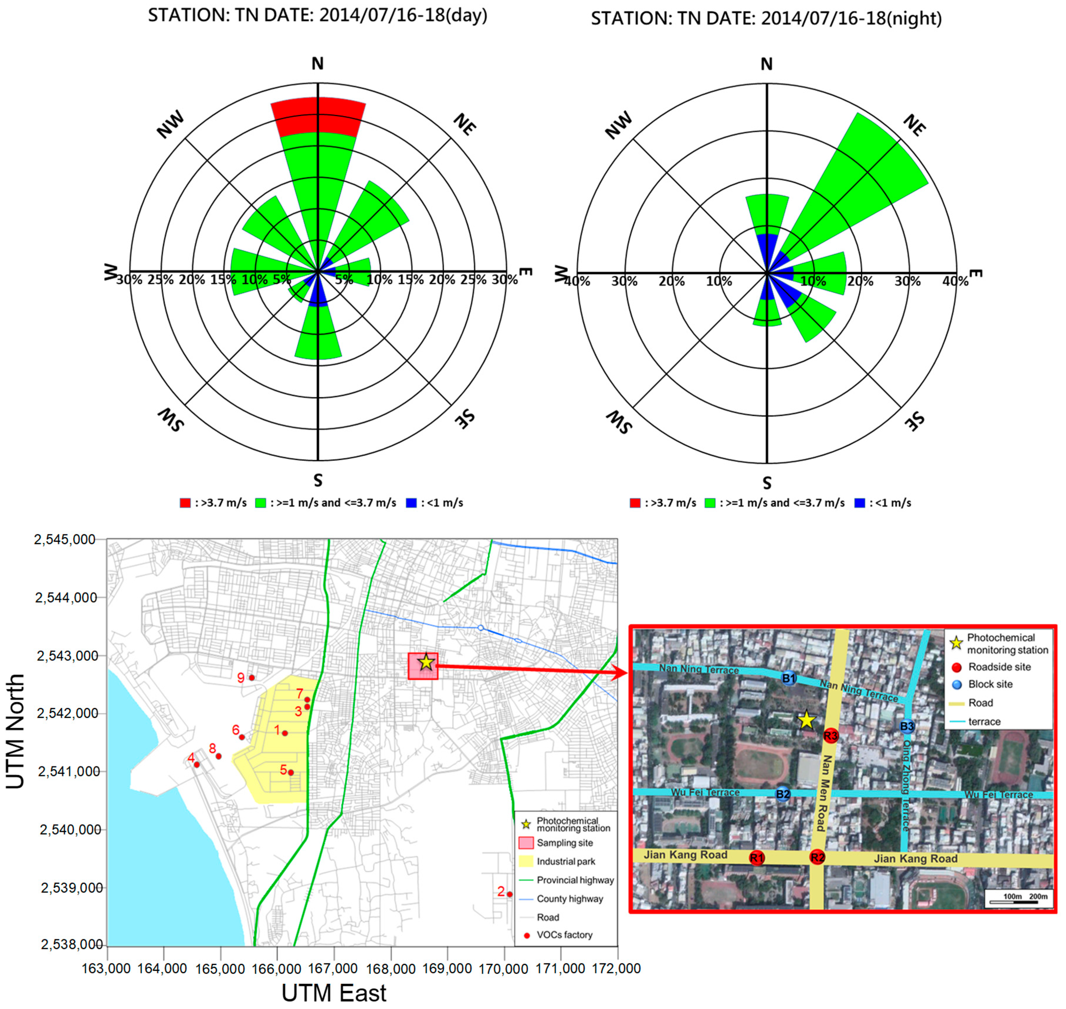
2.1. Sampling Sites and Period of Data Collection
2.2. VOC Analysis
2.3. Carbonyl Analysis
2.4. Ozone Formation Potential (OFP) of VOC Species
2.5. Risk Assessment
3. Results and Discussion
3.1. VOCs Characteristics
3.1.1. Roadside Sites
3.1.2. Residential Sites
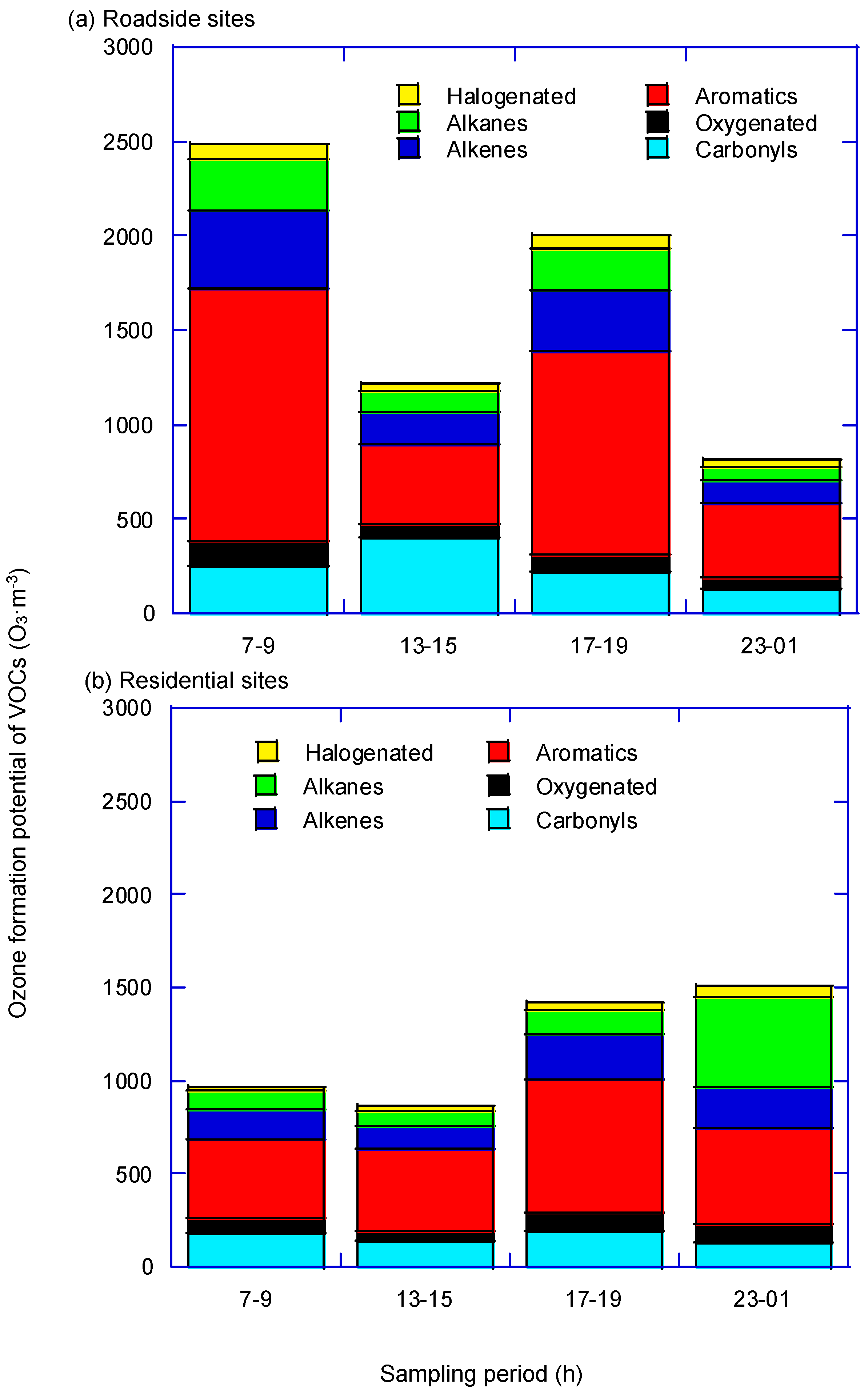
3.2. Ozone Formation Potential
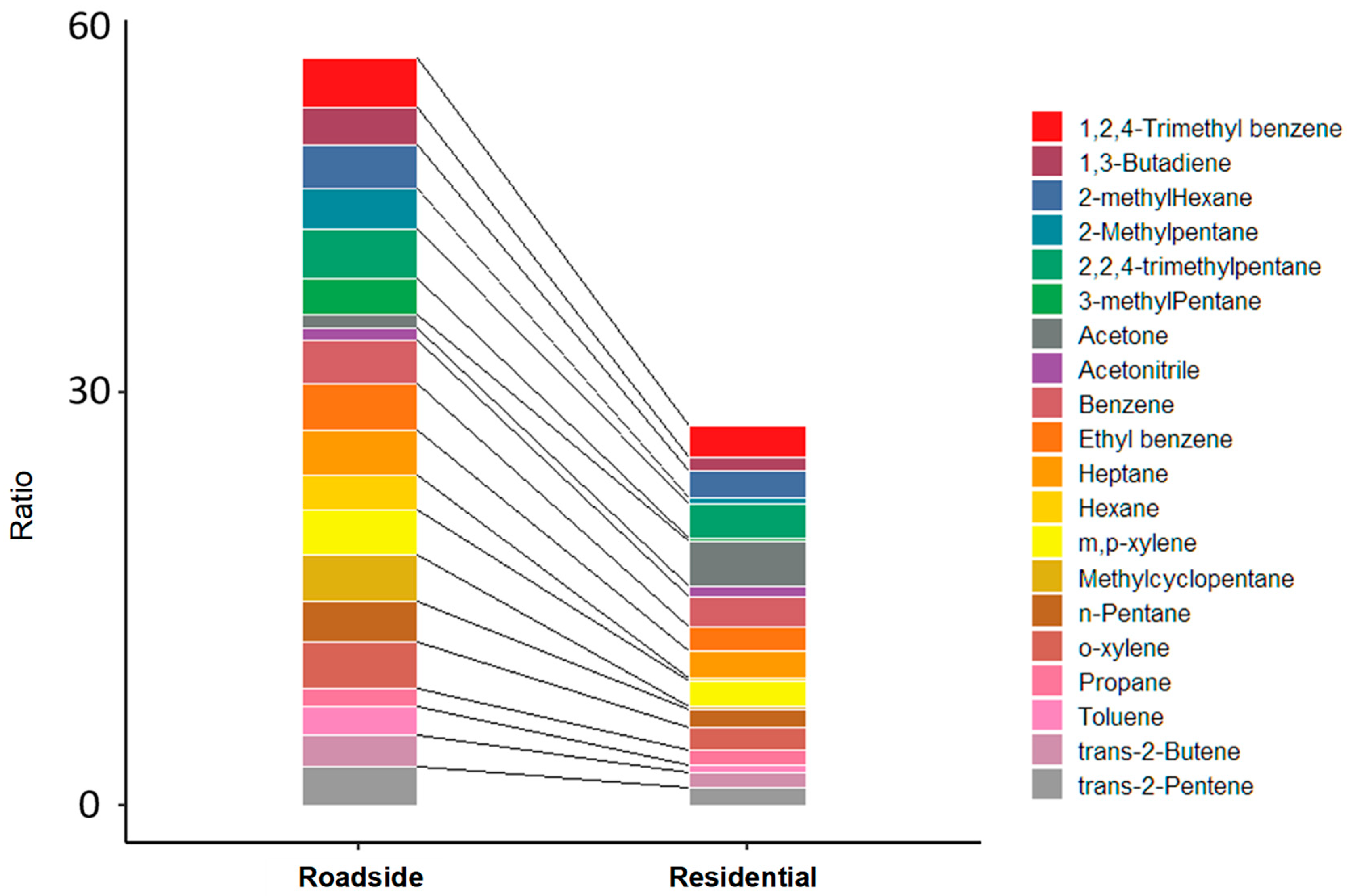
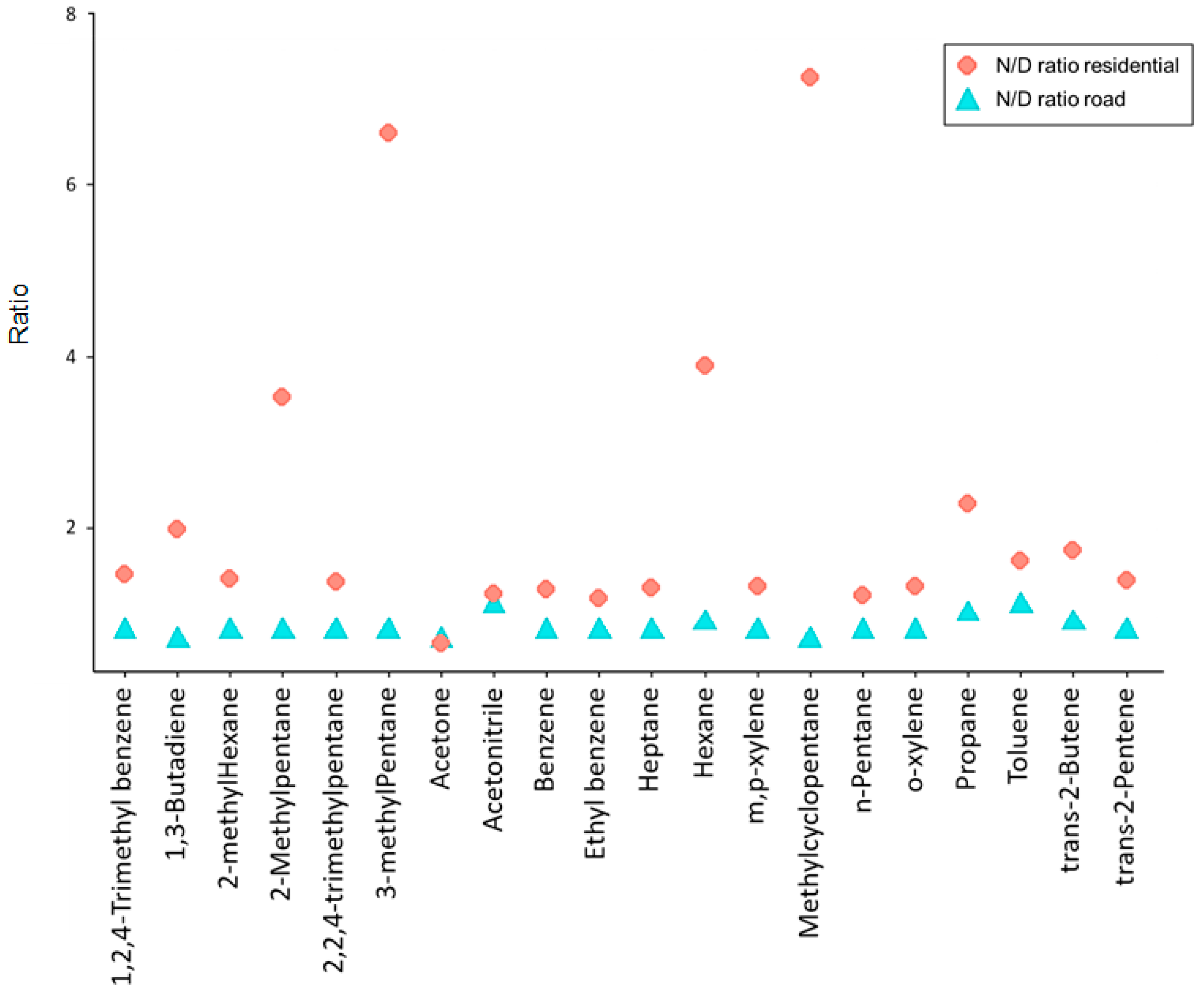
3.3. Ratio Analysis
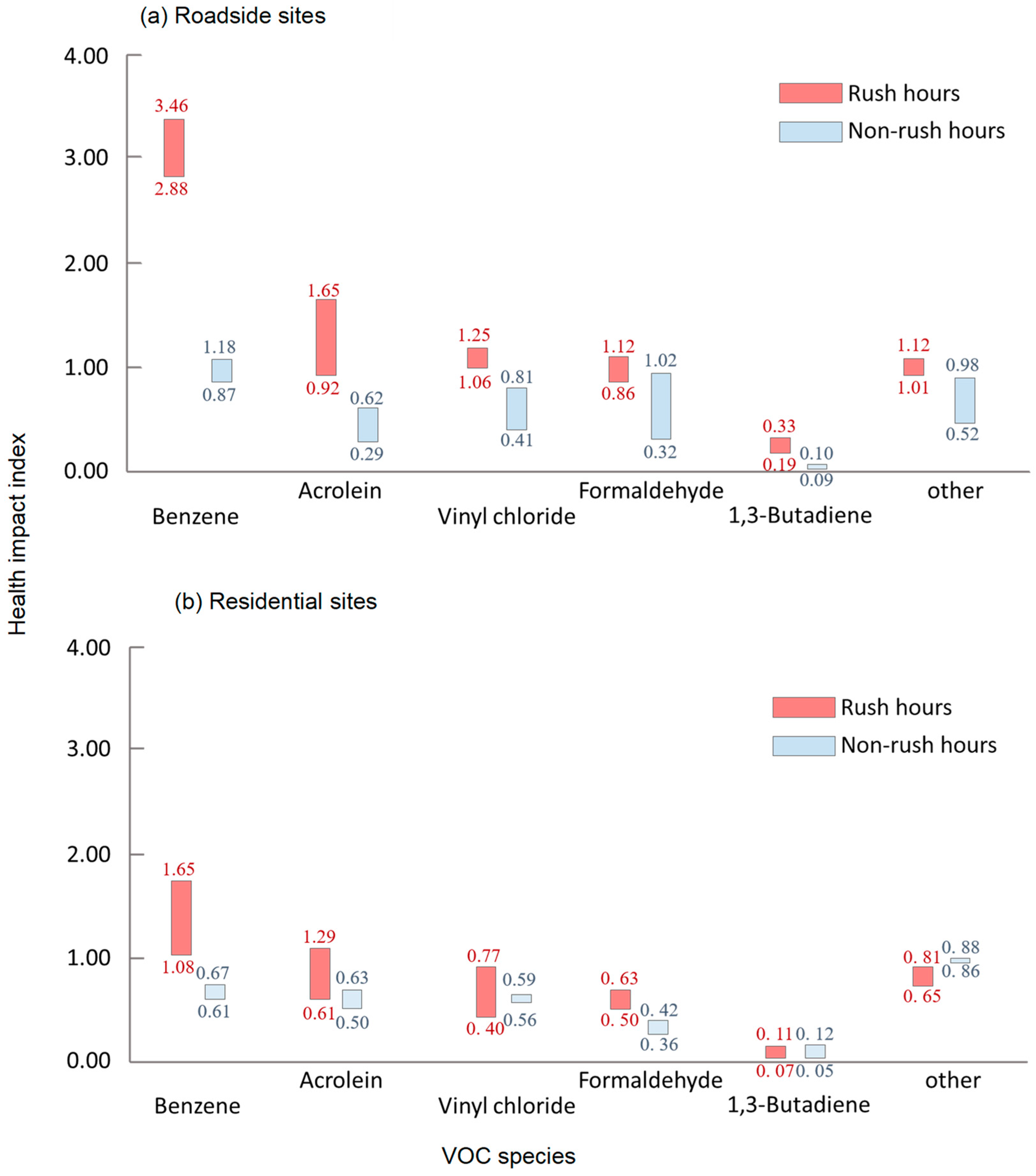
3.4. Health Impacts
3.4.1. Roadside Sites
3.4.2. Residential Sites
4. Conclusions
Supplementary Materials
Author Contributions
Funding
Acknowledgments
Conflicts of Interest
References
- World Health Organization. Health Risks of Air Pollution in Europe—HRAPIE Project; WHO: Copenhagen, Denmark, 2013. [Google Scholar]
- World Health Organization. Economic Cost of the Health Impact of Air Pollution in Europe: Clean Air, Health and Wealth; WHO Regional Office for Europe: Copenhagen, Denmark, 2015. [Google Scholar]
- European Environment Agency. Air Quality in Europe—2018 Report; EEA: Copenhagen, Denmark, 2018. [Google Scholar]
- US EPA. Cancer Risk from Outdoor Exposure to Air Toxics; EPA-450/1-90-004a; EPA: Research Triangle Park, NC, USA, 1990.
- Payne-Sturges, D.C.; A Burke, T.; Breysse, P.; Diener-West, M.; Buckley, T.J. Personal exposure meets risk assessment: A comparison of measured and modeled exposures and risks in an urban community. Environ. Health Perspect. 2004, 112, 589–598. [Google Scholar] [CrossRef] [PubMed] [Green Version]
- Jerrett, M.; Burnett, R.T.; Ma, R.; Pope, C.A.; Krewski, D.; Newbold, K.B.; Thurston, G.; Shi, Y.; Finkelstein, N.; Calle, E.E.; et al. Spatial Analysis of Air Pollution and Mortality in Los Angeles. Epidemiology 2005, 16, 727–736. [Google Scholar] [CrossRef] [PubMed]
- Ghosh, J.K.C.; Heck, J.E.; Cockburn, M.; Su, J.; Jerrett, M.; Ritz, B. Prenatal exposure to traffic-related air pollution and risk of early childhood cancers. Am. J. Epidemiol. 2013, 178, 1233–1239. [Google Scholar] [CrossRef]
- Wilhelm, M.; Ghosh, J.K.; Su, J.; Cockburn, M.; Jerrett, M.; Ritz, B. Traffic-Related Air Toxics and Term Low Birth Weight in Los Angeles County, California. Environ. Heal. Perspect. 2011, 120, 132–138. [Google Scholar] [CrossRef] [PubMed] [Green Version]
- Baker, A.K.; Beyersdorf, A.; Doezema, L.A.; Katzenstein, A.; Meinardi, S.; Simpson, I.J.; Blake, D.R.; Rowland, F.S. Measurements of nonmethane hydrocarbons in 28 United States cities. Atmos. Environ. 2008, 42, 170–182. [Google Scholar] [CrossRef] [Green Version]
- Garcia-Gonzales, D.A.; Shamasunder, B.; Jerrett, M. Distance decay gradients in hazardous air pollution concentrations around oil and natural gas facilities in the city of Los Angeles: A pilot study. Environ. Res. 2019, 173, 232–236. [Google Scholar] [CrossRef]
- Shah, R.U.; Coggon, M.M.; Gkatzelis, G.I.; McDonald, B.C.; Tasoglou, A.; Huber, H.; Gilman, J.B.; Warneke, C.; Robinson, A.; Presto, A.A. Urban Oxidation Flow Reactor Measurements Reveal Significant Secondary Organic Aerosol Contributions from Volatile Emissions of Emerging Importance. Environ. Sci. Technol. 2019, 54, 714–725. [Google Scholar] [CrossRef]
- USEPA. Available online: https://www.epa.gov/indoor-air-quality-iaq/volatile-organic-compounds-impact-indoor-air-quality#Health_Effects (accessed on 20 March 2020).
- Mohamed, M.F.; Kang, D.; Aneja, V.P. Volatile organic compounds in some urban locations in United States. Chemosphere 2002, 47, 863–882. [Google Scholar] [CrossRef]
- McDonald, B.C.; De Gouw, J.; Gilman, J.B.; Jathar, S.H.; Akherati, A.; Cappa, C.D.; Jimenez, J.L.; Lee-Taylor, J.; Hayes, P.L.; McKeen, S.A.; et al. Volatile chemical products emerging as largest petrochemical source of urban organic emissions. Science 2018, 359, 760–764. [Google Scholar] [CrossRef] [Green Version]
- The Government of the Hong Kong. Environmental Protection Department. Hong Kong Air Pollutant Emission Inventory—Volatile Organic Compounds. Available online: https://www.epd.gov.hk/epd/english/environmentinhk/air/data/emission_inve.html (accessed on 20 March 2020).
- Taiwan Central Weather Bureau (TCWB). Climate statistics. Available online: http://www.cwb.gov.tw/V7/climate/monthlyMean/Taiwan_tx.htm (accessed on 3 September 2020).
- US EPA. Determination of Volatile Organic Compounds (VOCs) in Air Collected in Specially—Prepared Canisters and Analyzed by Gas Chromatography/Mass Spectrometry(GC/MS). In Selected Analytical Methods for Environmental Remediation and Recovery (SAM); EPA: Cincinnati, OH, USA, 1999. [Google Scholar]
- US EPA. Reduction of Detection Limits to Meet Vapor Instrusion Monitoring Needs. In Compendium Method TO-15-Supplement; EPA: Research Triangle Park, NC, USA, 2009. [Google Scholar]
- US EPA. Compendium Method TO-11A. Determination of Formaldehyde in Ambient Air Using Adsorbent Cartridge Followed by High Performance Liquid Chromatography (HPLC); EPA: Cincinnati, OH, USA, 1999.
- Russell, A.; Milford, J.; Bergin, M.S.; McBride, S.; McNair, L.; Yang, Y.; Stockwell, W.; Croes, B. Urban Ozone Control and Atmospheric Reactivity of Organic Gases. Science 1995, 269, 491–495. [Google Scholar] [CrossRef] [Green Version]
- Carter, W.P.L. Updated Maximum Incremental Reactivity Scale and Hydrocarbon in Reactivities for Regulatory Applications; University of California: Riverside, CA, USA, 2009. [Google Scholar]
- Texas Commission on Environmental Quality (TCEQ). Air Toxics. Available online: http://www.tceq.state.tx.us/toxicology/AirToxics.html/#list (accessed on 15 May 2020).
- Doherty, R.E. A History of the Production and Use of Carbon Tetrachloride, Tetrachloroethylene, Trichloroethylene and 1,1,1-Trichloroethane in the United States: Part 1—Historical Background; Carbon Tetrachloride and Tetrachloroethylene. Environ. Forensics 2000, 1, 69–81. [Google Scholar] [CrossRef]
- Doherty, R.E. A History of the Production and Use of Carbon Tetrachloride, Tetrachloroethylene, Trichloroethylene and 1,1,1-Trichloroethane in the United States: Part 2—Trichloroethylene and 1,1,1-Trichloroethane. Environ. Forensics 2000, 1, 83–93. [Google Scholar] [CrossRef]
- Scheutz, C.; Durant, N.D.; Hansen, M.H.; Bjerg, P.L. Natural and enhanced anaerobic degradation of 1,1,1-trichloroethane and its degradation products in the subsurface—A critical review. Water Res. 2011, 45, 2701–2723. [Google Scholar] [CrossRef] [PubMed]
- Martin-Martinez, M.; Gómez-Sainero, L.; Alvarez, M.A.; Bedia, J.; Rodriguez, J.; Bedia, J. Comparison of different precious metals in activated carbon-supported catalysts for the gas-phase hydrodechlorination of chloromethanes. Appl. Catal. B Environ. 2013, 132, 256–265. [Google Scholar] [CrossRef]
- Kirchstetter, T.W.; Singer, B.C.; Harley, R.A.; Kendall, G.R.; Hesson, J.M. Impact of California Reformulated Gasoline on Motor Vehicle Emissions. 2. Volatile Organic Compound Speciation and Reactivity. Environ. Sci. Technol. 1999, 33, 329–336. [Google Scholar] [CrossRef] [Green Version]
- Grosjean, E.; Rasmussen, R.A.; Grosjean, D. Ambient levels of gas phase pollutants in Porto Alegre, Brazil. Atmos. Environ. 1998, 32, 3371–3379. [Google Scholar] [CrossRef]
- Zhang, Q.; Wu, L.; Fang, X.; Liu, M.; Zhang, J.; Shao, M.; Lu, S.; Mao, H. Emission factors of volatile organic compounds (VOCs) based on the detailed vehicle classification in a tunnel study. Sci. Total. Environ. 2018, 624, 878–886. [Google Scholar] [CrossRef]
- Kumar, A.; Singh, D.; Kumar, K.; Singh, B.B.; Jain, V.K. Distribution of VOCs in urban and rural atmospheres of subtropical India: Temporal variation, source attribution, ratios, OFP and risk assessment. Sci. Total. Environ. 2018, 613, 492–501. [Google Scholar] [CrossRef]
- Holzinger, R.; Jordan, A.; Hansel, A.; Lindinger, W. Automobile Emissions of Acetonitrile: Assessment of its Contribution to the Global Source. J. Atmos. Chem. 2001, 38, 187–193. [Google Scholar] [CrossRef]
- Hamm, S.; Warneck, P. The interhemispheric distribution and the budget of acetonitrile in the troposphere. J. Geophys. Res. Space Phys. 1990, 95, 20593. [Google Scholar] [CrossRef]
- Holzinger, R.; Jordan, A.; Lindinger, W.; Scharffe, D.H.; Schade, G.; Crutzen, P.J.; Warneke, C.; Hansel, A. Biomass burning as a source of formaldehyde, acetaldehyde, methanol, acetone, acetonitrile, and hydrogen cyanide. Geophys. Res. Lett. 1999, 26, 1161–1164. [Google Scholar] [CrossRef]
- US EPA. Health and Environmental Effects Profile for Acetonitrile; Environmental Criteria and Assessment Office, Office of Health and Environmental Assessment, Office of Research and Development: Cincinnati, OH, USA, 1985. [Google Scholar]
- Environment Canada (EC). Priority Substances List Assessment Report: Acrylonitrile. Canadian Environmental Protection Act, 1999; Environment Canada: Ottawa, ON, Canada, 2000. [Google Scholar]
- Liang, X.; Chen, X.; Zhang, J.; Shi, T.; Sun, X.; Fan, L.; Wang, L.; Ye, D. Reactivity-based industrial volatile organic compounds emission inventory and its implications for ozone control strategies in China. Atmos. Environ. 2017, 162, 115–126. [Google Scholar] [CrossRef]
- Sillman, S. The relation between ozone, NOx and hydrocarbons in urban and polluted rural environments. Atmos. Environ. 1999, 33, 1821–1845. [Google Scholar] [CrossRef]
- Elminir, H.K. Dependence of urban air pollutants on meteorology. Sci. Total. Environ. 2005, 350, 225–237. [Google Scholar] [CrossRef]
- De Sario, M.; Katsouyanni, K.; Michelozzi, P. Climate change, extreme weather events, air pollution and respiratory health in Europe. Eur. Respir. J. 2013, 42, 826–843. [Google Scholar] [CrossRef] [Green Version]
- Sheng, J.; Zhao, D.; Ding, D.; Li, X.; Huang, M.; Gao, Y.; Quan, J.; Zhang, Q. Characterizing the level, photochemical reactivity, emission, and source contribution of the volatile organic compounds based on PTR-TOF-MS during winter haze period in Beijing, China. Atmos. Res. 2018, 212, 54–63. [Google Scholar] [CrossRef]
- Li, Y.; Yin, S.; Yu, S.; Yuan, M.; Dong, Z.; Zhang, D.; Yang, L.; Zhang, R. Characteristics, source apportionment and health risks of ambient VOCs during high ozone period at an urban site in central plain, China. Chemosphere 2020, 250, 126283. [Google Scholar] [CrossRef]
- Elbir, T.; Cetin, B.; Cetin, E.; Bayram, A.; Odabasi, M. Characterization of volatile organic compounds (VOCs) and their sources in the air of Izmir, Turkey. Environ. Monit. Assess. 2007, 133, 149. [Google Scholar] [CrossRef]
- Yuan, B.; Shao, M.; Lu, S.; Wang, B. Source profiles of volatile organic compounds associated with solvent use in Beijing, China. Atmos. Environ. 2010, 44, 1919–1926. [Google Scholar] [CrossRef]
- Alfoldy, B.; Mahfouz, M.; Yigiterhan, O.; Safi, M.; Elnaiem, A.; Giamberini, S. BTEX, nitrogen oxides, ammonia and ozone concentrations at traffic influenced and background urban sites in an arid environment. Atmos. Pollut. Res. 2019, 10, 445–454. [Google Scholar] [CrossRef]
- Liu, P.-W.G.; Yao, Y.-C.; Tsai, J.-H.; Hsu, Y.-C.; Chang, L.-P.; Chang, K.-H. Source impacts by volatile organic compounds in an industrial city of southern Taiwan. Sci. Total. Environ. 2008, 398, 154–163. [Google Scholar] [CrossRef] [PubMed]
- Yang, H.-H.; Dhital, N.B.; Wang, Y.-F.; Huang, S.-C.; Zhang, H.-Y. Effects of short-duration vehicular traffic control on volatile organic compounds in roadside atmosphere. Atmos. Pollut. Res. 2020, 11, 419–428. [Google Scholar] [CrossRef]
- Wang, X.; Sheng, G.-Y.; Fu, J.-M.; Chan, C.-Y.; Lee, S.; Chan, L.Y.; Wang, Z.-S. Urban roadside aromatic hydrocarbons in three cities of the Pearl River Delta, People’s Republic of China. Atmos. Environ. 2002, 36, 5141–5148. [Google Scholar] [CrossRef]
- Na, K.; Kim, Y.P. Seasonal characteristics of ambient volatile organic compounds in Seoul, Korea. Atmos. Environ. 2001, 35, 2603–2614. [Google Scholar] [CrossRef]
- Zalel, A.; Yuval; Broday, D. Revealing source signatures in ambient BTEX concentrations. Environ. Pollut. 2008, 156, 553–562. [Google Scholar] [CrossRef] [PubMed]
- US EPA. Environmental Protection Agency, Locating and Estimating Air Emissions from Sources of 1,3-Butadiene; EPA: Morrisville, NC, USA, 1996; 454/R-96-008.
- Mullins, J.A. Industrial emissions of 1,3-butadiene. Environ. Health Perspect. 1990, 86, 9–10. [Google Scholar] [CrossRef]


| Sampling Periods | 07:00–09:00 | 13:00–15:00 | 17:00–19:00 | 23:00–01:00 | |
|---|---|---|---|---|---|
| Compounds | |||||
| Toluene | 16.41 ± 7.88 | 5.634 ± 1.72 | 14.73 ± 7.32 | 9.27 ± 10.83 | |
| Acetone | 13.67 ± 7.27 | 14.63 ± 7.45 | 10.47 ± 5.88 | 8.91 ± 3.56 | |
| Acetonitrile | 13.64 ± 8.88 | 11.04 ± 5.12 | 10.68 ± 9.50 | 17.20 ± 11.89 | |
| m,p-xylene | 10.75 ± 5.23 | 3.23 ± 1.46 | 8.75 ± 3.85 | 2.78 ± 1.27 | |
| n-Pentane | 8.73 ± 3.88 | 3.37 ± 1.25 | 7.72 ± 3.25 | 2.28 ± 0.97 | |
| 2-Methylpentane | 7.60 ± 3.26 | 2.72 ± 1.07 | 6.24 ± 2.67 | 2.02 ± 0.90 | |
| Hexane | 6.68 ± 2.43 | 2.76 ± 0.66 | 6.18 ± 1.38 | 2.22 ± 0.37 | |
| Methylcyclopentane | 5.45 ± 2.63 | 1.71 ± 0.77 | 4.17 ± 1.81 | 1.16 ± 0.58 | |
| 2,2,4-trimethylpentane | 5.03 ± 2.52 | 1.51 ± 0.73 | 4.14 ± 1.98 | 1.03 ± 0.48 | |
| Benzene | 4.84 ± 2.31 | 1.65 ± 0.72 | 4.04 ± 1.77 | 1.22 ± 0.61 | |
| o-xylene | 4.76 ± 2.31 | 1.39 ± 0.63 | 3.88 ± 1.71 | 1.16 ± 0.49 | |
| 3-methylPentane | 4.32 ± 1.74 | 1.78 ± 0.69 | 3.53 ± 1.27 | 1.22 ± 0.46 | |
| 1,2,4-Trimethyl benzene | 4.26 ± 2.15 | 1.19 ± 0.56 | 3.31 ± 1.52 | 0.92 ± 0.39 | |
| 2-methylHexane | 3.64 ± 1.73 | 1.17 ± 0.50 | 3.00 ± 1.36 | 0.93 ± 0.44 | |
| Heptane | 3.51 ± 1.68 | 1.12 ± 0.48 | 2.86 ± 1.18 | 0.88 ± 0.38 | |
| trans-2-Pentene | 3.40 ± 1.58 | 1.35 ± 0.58 | 2.74 ± 1.15 | 0.86 ± 0.35 | |
| Ethyl benzene | 3.16 ± 1.54 | 0.90 ± 0.40 | 2.46 ± 1.08 | 0.72 ± 0.30 | |
| Propane | 3.15 ± 2.31 | 2.27 ± 1.49 | 2.93 ± 2.70 | 2.42 ± 2.20 | |
| 1,3-Butadiene | 3.01 ± 0.78 | 0.89 ± 0.39 | 1.71 ± 0.69 | 0.84 ± 0.69 | |
| trans-2-Butene | 2.95 ± 1.36 | 1.42 ± 0.54 | 2.72 ± 1.06 | 1.00 ± 0.35 | |
| 20 species | 128.97 (69) * | 61.73 (66) | 106.25 (70) | 59.01 (74) | |
| 87 analyzed species | 186.56 ± 73.39 | 92.97 ± 23. 93 | 152.24 ± 33.17 | 79.54 ± 24.13 | |
| Sampling Periods | 07:00–09:00 | 13:00–15:00 | 17:00–19:00 | 23:00–01:00 | |
|---|---|---|---|---|---|
| Compounds | |||||
| Acetone | 30.38 ± 12.94 | 13.62 ± 10.26 | 25.52 ± 25.78 | 3.50 ± 3.70 | |
| Acetonitrile | 13.75 ± 8.36 | 12.35 ± 12.62 | 12.28 ± 4.81 | 20.14 ± 20.05 | |
| Toluene | 7.18 ± 2.14 | 12.17 ± 20.00 | 10.93 ± 5.92 | 20.42 ± 26.69 | |
| n-Pentane | 3.95 ± 1.99 | 3.18 ± 2.70 | 5.19 ± 2.62 | 3.51 ± 1.87 | |
| Hexane | 3.54 ± 0.68 | 3.67 ± 4.06 | 3.88 ± 1.84 | 24.28 ± 32.48 | |
| m,p-xylene | 3.19 ± 1.54 | 3.26 ± 3.93 | 6.35 ± 2.72 | 2.14 ± 1.53 | |
| 2-Methylpentane | 2.73 ± 1.26 | 1.73 ± 0.95 | 3.68 ± 1.77 | 12.00 ± 15.03 | |
| Propane | 2.29 ± 0.92 | 1.58 ± 0.61 | 4.06 ± 2.56 | 4.80 ± 1.99 | |
| 2-Butanone | 2.04 ± 0.80 | 1.71 ± 2.36 | 2.01 ± 0.85 | 2.16 ± 1.57 | |
| Methylcyclopentane | 1.95 ± 1.00 | 1.13 ± 0.65 | 2.40 ± 1.26 | 19.96 ± 27.33 | |
| Methylene chloride | 1.70 ± 0.89 | 2.64 ± 3.15 | 2.68 ± 1.12 | 1.67 ± 0.81 | |
| 3-methylPentane | 1.69 ± 0.74 | 1.23 ± 0.63 | 2.14 ± 0.99 | 17.09 ± 24.03 | |
| trans-2-Butene | 1.58 ± 1.19 | 1.16 ± 0.75 | 2.32 ± 1.18 | 0.68 ± 0.23 | |
| Benzene | 1.51 ± 0.65 | 0.94 ± 0.54 | 2.30 ± 1.06 | 0.85 ± 0.41 | |
| o-xylene | 1.45 ± 0.68 | 1.40 ± 1.60 | 2.68 ± 1.12 | 1.09 ± 0.78 | |
| 2,2,4-trimethylpentane | 1.38 ± 0.79 | 0.73 ± 0.47 | 2.21 ± 1.13 | 0.70 ± 0.28 | |
| Vinyl acetate | 1.35 ± 1.03 | 0.93 ± 0.76 | 1.73 ± 0.81 | 0.49 ± 0.48 | |
| trans-2-Pentene | 1.30 ± 0.87 | 0.97 ± 0.67 | 1.84 ± 0.92 | 1.32 ± 43 | |
| 1,2,4-Trimethyl benzene | 1.11 ± 0.64 | 0.62 ± 0.46 | 1.85 ± 0.93 | 0.68 ± 0.23 | |
| Chloromethane | 1.07 ± 0.14 | 0.92 ± 0.20 | 1.16 ± 0.34 | 1.16 ± 0.25 | |
| 20 species | 85.15 (80) * | 65.98 (76) | 96.53 (75) | 140.40 (83) | |
| 87 analyzed species | 106.43 ± 43.84 | 86.44 ± 51.99 | 129.48 ± 59.15 | 168.29 ± 154.05 | |
| City/Country | T/B | B/T | X/B | X/E | References | |
|---|---|---|---|---|---|---|
| Tainan (Taiwan) | RH-Roadside | 3.6 ± 0.62 | 0.3 ± 0.04 | 3.1 ± 0.29 | 5.1 ± 0.4 | |
| NRH-Roadside | 4.9 ± 2.91 | 0.3 ± 0.08 | 3.0 ± 0.35 | 5.3 ± 0.45 | This study | |
| RH-Residential | 4.8 ± 0.92 | 0.2 ± 0.03 | 3.6 ± 0.74 | 5.1 ± 0.46 | ||
| NRH-Residential | 12.4 ± 13.7 | 0.2 ± 0.12 | 4.0 ± 2.54 | 4.8 ± 0.79 | ||
| Taipei (Taiwan) | 5.8 | 0.4 | 1.5 | 2.9 | ||
| Kaohsiung (Taiwan) | Rush hour | 9.5 | 0.1 | 1.1 | 0.6 | [45] |
| Non-rush hour | 8.7 | 0.1 | 0.9 | 0.7 | ||
| Taichung (Taiwan) | 4.5–45.9 | - | 2.1–6.2 | 3.52–5.64 | [46] | |
| China, Japan, South Korea, Italy | 1.3–6.4 | 0.2–0.8 | 0.5–2.9 | 1.1–10 | [47,48] | |
| (a) Roadside | ||||||
|---|---|---|---|---|---|---|
| Items | PCU | TVOC | AMCVs | BC | PC | MT |
| PCU | 1 | |||||
| TVOC | 0.71 | 1 | ||||
| AMCVs | 0.82 | 0.99 * | 1 | |||
| BC | 0.94 | 0.52 | 0.65 | 1 | ||
| PC | 0.98 * | 0.57 | 0.7 | 0.97 * | 1 | |
| MT | 0.94 | 0.9 | 0.96 * | 0.79 | 0.86 | 1 |
| (b) Residential | ||||||
| PCU | 1 | |||||
| TVOC | −0.48 | 1 | ||||
| AMCVs | 0.82 | 0.1 | 1 | |||
| BC | −0.08 | −0.69 | −0.47 | 1 | ||
| PC | 0.94 | −0.49 | 0.78 | 0.15 | 1 | |
| MT | 0.97 * | −0.39 | 0.82 | −0.27 | 0.84 | 1 |
© 2020 by the authors. Licensee MDPI, Basel, Switzerland. This article is an open access article distributed under the terms and conditions of the Creative Commons Attribution (CC BY) license (http://creativecommons.org/licenses/by/4.0/).
Share and Cite
Tsai, J.-H.; Lu, Y.-T.; Chung, I.-I.; Chiang, H.-L. Traffic-Related Airborne VOC Profiles Variation on Road Sites and Residential Area within a Microscale in Urban Area in Southern Taiwan. Atmosphere 2020, 11, 1015. https://doi.org/10.3390/atmos11091015
Tsai J-H, Lu Y-T, Chung I-I, Chiang H-L. Traffic-Related Airborne VOC Profiles Variation on Road Sites and Residential Area within a Microscale in Urban Area in Southern Taiwan. Atmosphere. 2020; 11(9):1015. https://doi.org/10.3390/atmos11091015
Chicago/Turabian StyleTsai, Jiun-Horng, Yen-Ting Lu, I-I Chung, and Hung-Lung Chiang. 2020. "Traffic-Related Airborne VOC Profiles Variation on Road Sites and Residential Area within a Microscale in Urban Area in Southern Taiwan" Atmosphere 11, no. 9: 1015. https://doi.org/10.3390/atmos11091015