Article

Variability and Trend in Integrated Water Vapour from ERA-Interim and IGRA2 Observations over Peninsular Malaysia

by
Ezekiel Kaura Makama
1,2,* and
Hwee San Lim
1,*
1
School of Physics, Universiti Sains Malaysia, Pulau Pinang USM 11800, Malaysia
2
Department of Physics, University of Jos, PMB 2084 Jos, Nigeria
*
Authors to whom correspondence should be addressed.
Atmosphere 2020, 11(9), 1012; https://doi.org/10.3390/atmos11091012
Submission received: 30 July 2020 / Revised: 28 August 2020 / Accepted: 2 September 2020 / Published: 22 September 2020
(This article belongs to the Section Meteorology)

Abstract

:
Integrated water vapour (IWV) is the total amount of precipitable water in an atmospheric column between the Earth’s surface and space. The implication of its variability and trend on the Earth’s radiation budget and precipitation makes its monitoring on a regular basis important. ERA-Interim reanalysis (ERA) and radiosonde (RS) data from 1988 to 2018 were used to investigate variability and trend in IWV over Peninsular Malaysia. ERA performed excellently when gauged with RS. Trend analysis was performed using the non-parametric Mann–Kendall and Theil–Sen slope estimator tests. ERA and RS IWV revealed double fluctuations at the seasonal time scale, with maxima in May and November, which are the respective beginnings of the southwest monsoon (SWM) and northeast monsoon (NEM) seasons, as well as coincidental peaks of precipitation in the region. IWV decreased in a southeast–northwest orientation, with regional maximum domiciled over the southeastern tip of the region. Steep orography tended to shape intense horizontal gradients along the edges of the peninsular, with richer gradients manifesting along the western boundary during SWM, which harbours more water vapour in the peninsular. IWV trends, both at the annual and seasonal time series, were positive and statistically significant at the 95% level across the stations, except at Kota Bharu, where a nonsignificant downward trend manifested. Trends were mostly higher in the NEM, with the greatest rate being 0.20 ± 0.42 kgm−2 found at Penang. Overall, the IWV trend in Peninsular Malaysia was positive and consistent with the upward global changes in IWV reported elsewhere.

1. Introduction

Precipitable water vapour or simply, precipitable water, is the gaseous phase of water in the Earth’s atmosphere, formed from the constantly changing phases of water within the range of normal atmospheric temperatures. Although precipitable water represents a small percentage (0–4%) of the entire atmospheric gas constituents, it is arguably the most abundant and most influential of the entire major greenhouse gases in the atmosphere [1]. It provides strong positive feedback for global warming [2] and plays vital roles in climate change, hydrological processes, Earth’s energy balance, and weather systems [3]. Precipitable water exhibits higher spatial and temporal variability than the other greenhouse gases [1], with values up to 50 mm near the equator and lower than as much as one-tenth at the poles. Its average resident time is 8 days, with the tropical convergence zones condoning it for about 12 days [4]; its residency at subtropical high regions is much shorter.
The high spatial and temporal variations of precipitable water in the atmosphere call for its regular and accurate monitoring for climatological and meteorological purposes [5]. Its quantification, in both the real atmosphere and climate models, is particularly significant in understanding water vapour feedback on global warming. Knowledge of the total vertical column of this parameter, also known as integrated water vapour (IWV), and its variations, is particularly more useful than surface humidity in the studies of radiation budget and the forecast of precipitation [6]. IWV variability and trends, which are also significant in the exploration of climate change [7], form the central objective of this study.
In recent years, many studies have been carried out to probe and detect changes in IWV by deploying a variety of datasets retrievable from different sensors or platforms, including radiosonde [8,9], microwave radiometers [10], Global Positioning Systems (GPS) [11,12,13], Raman Lidar [14], and satellite remote sensing [15]. Traditionally, observation records from radiosondes represent an important resource for monitoring the variability and trends in IWV because of its accuracy and vertical resolution. It is not surprising, therefore, that observational records from this platform have been used by many scholars as reference data in gauging the validity of IWV obtained from other techniques [16]. For instance, the authors in [17] reported bias and root mean square errors of 0.68 and 4.47 kgm−2, respectively, for global tropical region when they evaluated ERA-Interim IWV against the radiosonde product.
Many previous studies, using data from different platforms or sensors, have revealed both region and time scale IWV trends. For instance, Rose and Elliott [18] used radiosonde observations to establish an upward trend in IWV across most sites in the United States and Canada between 1973 and 1993. Similar positive trends, mostly in the Northern Hemisphere, have been reported [3,19]. Based on 27-year radiosonde observations in China, Xie et al. [20] also reported a significant upward IWV trend from 1979 to 2005 in the northern part of China, with a reversed trend in the southern part. Similarly, Chen and Liu [17] deployed precipitable water datasets from radiosonde, European Centre for Medium-range Weather Forecast (ECMWF), National Centre for Environmental Prediction (NCEP) reanalysis, GPS, and microwave satellite observations, for the period 1979–2014, to analyse both variability and trend in global precipitable water and obtained positive global trends for all five datasets. Generally, research efforts have pointed to upward water vapour trends, both at the surface [1,3,18] and aloft [3].
On average, precipitable water vapour content appears to produce positive trends globally, consistent with global warming. However, such inferences may not be absolute, since various studies deployed data from different sources and sites, with varying temporal and spatial coverages. More so, most techniques or sensors deployed in gathering humidity data for the quantification and/or trend analyses of IWV cited above suffer one form of limitation or the other. For instance, the data quality of radiosonde networks is not only variable in the upper troposphere, but poor at extreme humidity values [18]. Spatial limitations due to high operational cost and differences in instruments’ sensors over time add to the heterogeneity of the network’s data quality. While observations from sun photometers are limited to cloud-free regions, low spatial resolution restricts the use of space-based instruments. Since the introduction of GPS as an efficient meteorological tool by [11], its data are frequently used to determine precipitable water, among other atmospheric parameters. The temporal span of GPS data, however, falls short of the minimum period (30 years) required to aggregate weather for the evaluation of climatic effects in an area, as described by the World Meteorological Organization (WMO) [21]. This period is deemed sufficiently long to filter interannual variations or anomalies and thus, reveal climatic trends [22]. Due to frequent changes in data assimilation systems and models, operational analyses from in situ and satellite observations are rather short in providing homogeneous datasets on the atmospheric moisture budget. Retroactively produced (reanalysis) data, based on the utilisation of the same model and data assimilation procedure, are, therefore, better in this respect [23]. Reanalysis datasets for atmospheric studies are produced by assimilating various types of observations (ground and satellite) into a dynamically coherent dataset based on an atmospheric general circulation model [24]. These datasets have been widely used in atmospheric studies like climate change because they have the advantages of multivariable outputs, global coverage, and continuous records.
The foregoing relevance of IWV in climate studies, amongst others, has endeared interests in its measurement and evolution, both in space and time. Regrettably, however, the study of IWV variability and trend in Peninsular Malaysia is rare despite being an area characterised by various climatic features [25]. Aside from the very few reports on the quantification of IWV in the area, e.g., [26], there are no existing studies on its variability and trend, let alone the deployment of ERA-Interim reanalysis data. This is probably due to the limited number of in situ stations with traditionally long periods of data records for meaningful exploration of variability and trends in IWV, unlike other regions in the mid-latitude of the Northern Hemisphere. Peninsular Malaysia is an important area for climate study, being a tropical region with overlapping seasonality and high topographic inhomogeneity. Moreover, many global and regional phenomena, like El Niño, La Niña, and Indian Ocean Dipole, are thought to influence the climate of the peninsular in addition to global warming. These proponents could affect the severity of extreme events in the country [27]. Peninsular Malaysia, which stretches from longitude 99–105° east of the meridian and from latitude 1–7° north of the equator, exhibits two main seasons, the northeast monsoon (NEM) and southwest monsoon (SWM), flanked by two inter-monsoon characteristics.
The research area, which is situated in the equatorial doldrum region, is also characterised by almost constant temperature year-round, having values between 24 and 32 °C, with annual variation of ~2 °C. However, the east coast is often affected by cold surges originating from Siberia during the NEM [28,29]. Vector winds and temperature patterns for the SWM and NEM seasons in the study area are shown in Figure 1. The topography of Peninsular Malaysia is characterised by a series of mountains, rising abruptly from the wider and flatter coastal plains. Prominent among these undulating surfaces is the Titiwangsa Mountains, which run from the Malaysia–Thailand border in the north to the southern state of Negeri Sembilan, effectively demarcating the area into western and eastern parts, as shown in the inset of Figure 2. These mountains exert considerable influence on the local wind circulations in the region.
In the current study, therefore, both radiosonde data from the Integrated Global Radiosonde Archive (IGRA) version 2 and the ERA-Interim reanalysis product from ECMWF [30] for the period 1988–2018 are used to investigate variability and trends in IWV over Peninsular Malaysia. ERA is one of the most advanced global atmospheric reanalysis records, which has been revised and improved upon over the years and used elsewhere to evaluate both variability and trends in IWV [5,7,19,30]. Moreover, the data compare well with radiosonde observations [31]. This paper focuses on the evaluation of the annual and seasonal means of IWV as well as its variations and long-term trends over Peninsular Malaysia. Though analysis of seasonal variability helps to better identify regions with higher uncertainty as well as understand the physical processes involved in different seasons (e.g., the component responsible for moisture advection differs in wet and dry seasons) [31], it is rarely provided in many other studies. In the current paper, interannual and seasonal (NEM and SWM) variability in ERA and RS IWV are evaluated over Peninsular Malaysia. IWV observations from the Advanced Television and Infrared Observation Satellite Operational Vertical Sounder (ATOVS) are primarily used to evaluate the spatial representation of ERA IWV in the study region. Prior to long-term trend analysis, the IWV from ERA is firstly compared with: (1) Retroactively produced IWV retrieved from ATOVS instruments aboard the National Oceanic and Atmospheric Administration (NOAA) and archived by the Satellite Application Facility on Climate Monitoring (CM-SAF), for the period 2001–2011. (2) Radiosonde IWV (RS) observations from IGRA (1988–2018) for selected WMO stations within and around Peninsular Malaysia. The paper is organised such that data description and methodology are detailed in Section 2, while the results are presented and discussed in Section 3, with conclusions drawn in Section 4.

2. Data and Methodology

The variability and trend studies of IWV are performed using 31 years of monthly means of ERA and RS observations. The study area is shown in Figure 2, with the locations of IGRA stations represented by dark-filled diamonds. Prior to the foregoing analyses, ERA IWV is compared with RS and CM-SAF (SAF) IWV records. The coefficient of determination (R2), mean bias (MB), and root mean square (RMS) errors have been used to gauge the level of agreement between the different pairs of datasets. The sources, description, and methodologies used in acquiring the respective datasets are described below.

2.1. Radiosonde

Daily radiosonde data for this study were obtained from the Integrated Global Radiosonde Archive (IGRA) version 2 of the National Climatic Data Centre (NCDC, Asheville, NC, USA). The data are available [32]. IGRA2 consists of almost 2700 global stations for both radiosonde and pilot balloon observations, with a temporal span of over 60 years of records, which include temperature, relative humidity, pressure, wind speed, and wind direction. The requisite IWV data were extracted from twice-daily radiosonde observations at mandatory and significant levels from WMO stations at Kota Bharu, Penang, Kuantan, Sepang, and Changi (Singapore) for the period 1st January 1988 to 31st December 2018. The datasets were retrieved along with metadata on background instrumentation and station history, which helped in ensuring data quality through checks for inconsistencies such as outliers and duplicate levels, among others.
Three stages of quality control were imposed on the daily data: Firstly, obvious errors, e.g., values of IWV <20 and >100 mm were discarded as invalid. Secondly, the monthly and annual mean values of IWV for each station were calculated based on outputs from the first stage. Finally, outliers were removed from the time series of eventual stations when the difference between their values and the climatological mean was more than 3 standard deviations (σ) [33]. The systematic as well as instrumental errors were, however, not considered in the quality control process. After the quality control procedure, the data were further tested for homogeneity as follows: (1) Stations with obvious inhomogeneous data were not considered. (2) Stations without complete twice daily records were precluded. (3) At least 18 daily observations were used to calculate the mean monthly values. Any year that had at least 10 valid months was used in deriving the mean values of IWV. (4) Data from stations with a consistent time series of 11 years between 1988 and 2018 were considered for variational studies, while a minimum of 19 years of data was used for trend analysis. After the homogeneity test, records from four of the six WMO stations in Peninsular Malaysia were found useful in the computation of IWV values for comparison with the ERA observations. Data from Changi airport in Singapore, which lies at the fringe of the southern part of the study area, were equally subjected to quality examination and found useful for inclusion in the inter-comparison and trend analysis.
The diurnal (1200 UTC) and nocturnal (0000 UTC) data were separately treated and found to correlate excellently across the stations, with correlation coefficient r ≥ 0.93. Although, insignificant differences in trend between 0000 and 1200 UTC have been reported [18]. Nonetheless, the daily value was derived as the mean of the two observations for each day and then, converted into monthly means to conform with those of ERA-Interim. Information on the data used, including station location, are given in Table 1.

2.2. CM-SAF from ATOVS

Homogenised satellite data records, SAF, were mainly used to validate ERA. This set of data is retrieved and archived by CM-SAF from ATOVS instruments aboard NOAA and Meteorological Operational (Metop) Satellites. The ATOVS suite of instruments, which comprises a High-Resolution Infrared Radiation Sounder (HIRS), Advanced Microwave Sounding Unit A and B (AMSU-A/B), and Microwave Humidity Sounder (MHS), represents infrared spectrometers and microwave radiometers. These instruments contain enough information to infer IWV value. Retrievals over oceans rely on all sensors, whereas retrievals over land surfaces are mainly based on cloud-free HIRS measurements. On a global scale, radiosondes and ATOVS water vapour agree reasonably well, with systematic differences of 0.5 kg m−2 and root mean square differences of approximately 4 kg m−2 [34]. The ATOVS data records consist of precipitable water and temperature products defined at all longitudes and for latitudes 80° N to 80° S. CM-SAF retrieves and provides global fields of daily mean IWV on a cylindrical equal area projection of 90 × 90 km2 and 0.5 × 0.5 longitude–latitude grid. The dataset is accompanied by an uncertainty estimate that reflects the retrieval uncertainty and the sampling error, which is particularly important in tropical areas. They are constructed using a specific kriging algorithm that is detailed in Li et al. [35] and expounded by Schröder et al. [15]. In this study, SAF data, for the period 2001–2011, also known as a climate data record (CDR), were extracted for all available latitudes over the entire study area shown in Table 1 and Figure 1. Though the CDR spans 13 years, the first two years are plagued with so many temporal gaps and are, therefore, precluded in this study. This set of data, freely ordered from the CM-SAF website [35] contain high-quality, validated, homogeneous climate data based on carefully calibrated inter-sensor radiances. The daily data from 2001 to 2011 were re-gridded to 0.125° × 0.125° longitude–latitude and converted to mean monthly array for compatibility with the ERA IWV data.

2.3. ERA-Interim Reanalysis

ECMWF initiated a project to bridge her previous reanalysis, ERA-40, which spanned 1957–2002, with her next-generation extended reanalysis, ERA-Interim. The aim of the project was to improve on vital aspects of the former. This success resulted from a combination of factors, which include the use of 4D variational analysis to minimise errors, the use of variational bias correction for satellite data (impact of observing system changes is reduced), and other improvements in data handling. With the improvement, ERA can now incorporate regular and irregular meteorological data, offer better humidity analysis, as well as effective representation of the hydrologic cycle and stratospheric circulation. The product, a global atmospheric reanalysis of repute, is available from 1st January 1979 to 31st August 2019 and can be downloaded freely from the ECMWF Public Datasets web interface [36]. The IWV products from the ERA reanalysis are based on various water vapour measurements, which include clear-sky radiance observations from geostationary and polar-orbiting sounders, and the images of remote sensing satellites like the Special Sensor Microwave Imager (SSM/I), Total Ozone Mapping Spectrophotometer (TOMS), TIROS Operational Vertical Sounder (TOVS), and High Resolution Infrared Radiation Sounder. Detailed documentation is found in [30]. ERA has been used in several climate and trend analysis studies [15,17]. A stream of monthly means IWV of daily means data at a 0.125° × 0.125° resolution in netCDF output for the extent of Peninsular Malaysia (see Table 1) was retrieved for the period 1st January 1988 to 31st December 2018. A total of 372 mean monthly arrays, each consisting of 97 columns and 73 rows of IWV, were available for the evaluation of variability and trends.

2.4. Inter Comparison of Means and Variability of IWV

Precise knowledge of the accuracy of IWV derived from models prior to deploying reanalysis data for trend evaluation is indispensable. As stated earlier, RS and SAF can measure, with acceptable accuracy of the order of several millimetres, atmospheric water vapour contents. A validation of the ERA IWV is, therefore, performed using RS and SAF observations to obtain a reliable interpretation of the ERA data quality in the study area. Makama and Lim [25] obtained good agreement between radiosonde IWV and CM-SAF IWV, with correlation coefficients ranging between 0.79 and 0.94 with MB < 1 kgm−2 across different regions of Peninsular Malaysia when the two datasets were compared. ERA is firstly interpolated onto the radiosonde sites to extract the IWV data and then, directly compared with IWV measured at the stations. Five radiosonde stations were identified for this study (see Figure 1 and Table 1) for both the comparison and trend evaluations. Secondly, the SAF data were re-gridded to match the ERA grids and direct comparison of the means applied. It is worthy of note that SAF and RS IWV agree reasonably well in the current study area [25]. Unfortunately, only 11 years (2001–2011) of this dataset were used for validation for the reason mentioned in Section 2.2. Standard statistical metrics, MB and RMS errors, given in Equations (1) and (2), were used to validate ERA IWV against its RS and SAF counterparts across the study area.
M B = 1 n i = 1 n ( I W V I W V )
R M S = 1 n i = 1 n ( I W V I W V ) 2
where IWV is integrated water vapour derived from ERA, IWV′ is integrated water vapour from either RS or SAF observations, n is the number of data points, while I W V ¯ and I W V ¯ represent the respective mean values of the integrated water vapour from a pair of datasets.

2.5. Trend Analysis

Annual and seasonal trends were computed for each station from 1988 to 2018 in both the ERA and RS time series. Monthly anomalies were computed as deviations from the corresponding long-term monthly means over the 31-year period. Annual averages were then obtained from the monthly anomalies, with at least 10 months of data required for each annual anomaly. Time series for seasonal anomalies were similarly obtained for the NEM (November–April) and the SWM (May–October) by averaging the monthly anomalies for that season, with at least four months required for each seasonal anomaly. To detect the trend in the IWV time series, a non-parametric Mann–Kendall (M–K) test at 95% confidence level was imposed on both datasets. M–K, which is a rank-based process, applicable even in skewed data, has been widely used in detecting monotonic trends in climate study [32,37]. An additional major benefit of this test in analysing temporal series is that cases of missing data and seasonality are not considered.
Suppose integrated water vapour is observed over a time series x = x i , with i = 1 , 2 , 3 , , n as data points and x j being the data point at time j , then the M–K test statistic (S) is given as
S = i = 1 n 1 j = i + 1 n s g n ( x j x i )
where n is the sample size, while x i and x j are the respective values for years i and j, with j > i . The values of the data are treated based on an ordered time series evaluation, where each value is compared with all subsequent data values. The initial value of S is assumed to be 0 when there is no trend and 1 or −1 when there is an upward or downward trend, respectively. Simply put, if the value of a data point is higher or lower than the value that precedes it, then S is respectively incremented or decremented by 1. S is, therefore, defined by the sign function, with values ranging between ± 1 , depending on whether x j x i is less, equal, or greater than zero, as given in Equation (4) [37].
s g n ( x j x i ) = { + 1 , ( x j x i ) > 0 0 , ( x j x i ) = 0 1 , ( x j x i ) < 0
For a sample size upward of 30, the S statistic is normally distributed and the normalised test statistic Z can be computed as follows:
Z = { S 1 σ S , S > 0 0 , S = 0 S + 1 σ S , S < 0
The procedure for the M–K trend test assumes the existence of only one data value at a particular time period. If, however, there is more than one data point (tie) in a given time period, the median value is considered [38]. It is, however, important to calculate the probability associated with S and the sample size n, to statistically determine the significance or otherwise of the trend. The value of the variance of S (σ) was, therefore, obtained using Equation (6) [37] with n ≥ 10,
σ ( S ) = 1 18 [ n ( n 1 ) ( 2 n + 5 ) p = 1 m t p ( t p 1 ) ( 2 t p + 5 ) ]
where m is number of tied groups (i.e., a set of sample data with same value), and tp is the number of data points in the pth group. The probability associated with the variance was computed using Equation (7) in XLSTAT (XLSTAT is a complete analysis and statistics add-in for Microsoft Excel). This method is suitable for the IWV dataset in the current study, since the sample size is greater than 10 with very few ties.
f ( Z ) = e Z 2 / 2 2 π
The Z score considers the detection of monotonic trends from the following hypothesis: null hypothesis (H0)—no monotonic trend (i.e., variables are independent and equally distributed) and the alternative hypothesis (H1)—monotonic trend exists (i.e., variables are dependent with inhomogeneous distribution). The acceptance or otherwise of H0 is determined by computing the normalised probability associated with the Z statistic from Equation (6). In this paper, the significance level (α) was set at 0.05 (i.e., 95% confidence level) such that Z > | Z α / 2 | indicates no monotonic trend in the IWV data. H0 is, therefore, rendered invalid when | Z 0.025 | 1.96 , meaning that the trend is significant.
In this study, the Theil–Sen (T–S) estimator, which is resistant to outliers, was used to determine the magnitude of IWV trend. T–S, named after Henri Theil [39] and Pranab Sen [40], is a non-parametric method usually deployed in finding a fit for heteroscedastic data. Suppose ( t 1 , y 1 ) ,   ( t 2 , y 2 ) ,   ,   ( t n , y n ) represent data points, then T–S estimates the slope of the line that connects each pair of data. The median among the slopes of all the data pairs becomes the slope of the fit, given as
β ^ = m e d 1 i < j n y j y i t j t i
Knowing the value of the slope, the intercept was calculated as b ^ = y i β ^ t i , where t is time of observation. The sign of β ^ reveals whether the change is positive or negative and its magnitude shows how steep the change is [41].

3. Results and Discussion

3.1. Comparison of IWV from ERA with RS and SAF Observations

The comparison between monthly means IWV from ERA with those from RS and SAF was done using the statistical evaluation metrics provided in Equations (1) and (2). The objective here is to check the reliability and consistency of the ERA observations against RS and SAF measurements, as mentioned earlier. Again, note that SAF, being available from 2001 to 2011, was only used in the validation of ERA and not in long-term trends, due to its temporal limitation.

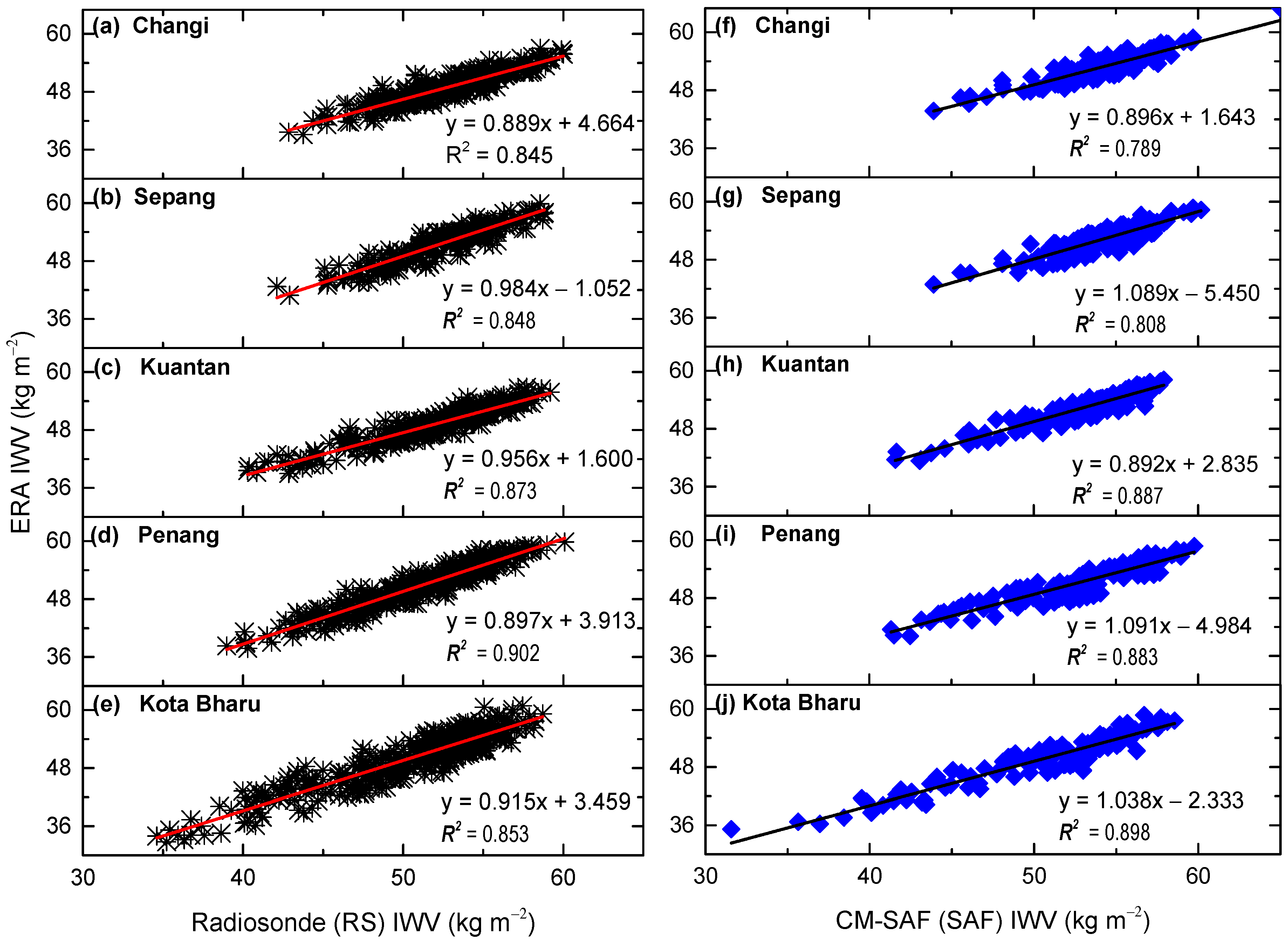
3.1.1. Evaluation of IWV Means

The comparison between the means of IWV from ERA, RS, and SAF for the five stations is summarised in Table 2, with the visual fits depicted in Figure 3. Table 2 presents values of the statistical indices for each of the five stations, including the number of observations, when the monthly means of IWV from RS and SAF were compared with those from ERA for the entire study period. Figure 3, on the other hand, shows the corresponding scatterplots for the monthly means of IWV from RS and SAF against those from ERA. On the bases of MB (Table 2), ERA is wet against RS and dry against SAF, with respective greatest values of −2.85 kg m−2 found at Changi and 1.94 kg m−2 at Sepang. While the average MB for all the stations in the RS/ERA comparison is well below 1 kg m−2, that of Changi is up by a scale of ~3. In the SAF/ERA comparison, the average MB is ~1.22 kg m−2 across all stations, with the smallest and largest values being 0.63 and 1.94 kg m−2 in Kuantan and Sepang, respectively. From the goodness of fits in Table 2, a proximity between the IWV from ERA and those from RS and SAF across all stations are revealed, except for a relative departure at Changi, where highest RMS for RS/ERA and SAF/ERA are 4.05 and 2.43 kg m−2, respectively. Moreover, the slopes in Figure 3 are close to 1, indicating that the data points are distributed around the 1:1 line, and the maximum deviations of ERA are less than two standard deviations from the means of both the RS and SAF. The slopes of the linear regression lines for the RS/ERA comparison shown in Figure 3 (left panel) are all below 1, ERA on average being wetter than RS with relatively larger differences at lower IWV values. A likely reason is the impairment of time-lag response suffered by radiosonde sensors as they ascend the atmosphere, during which IWV is underestimated [42]. However, the slopes of the linear fits for the SAF/ERA pairing, shown on the right panel in Figure 3, are above 1 for Kota Bharu, Penang, and Sepang, ERA being persistently drier particularly at higher IWV. This is probably due to the interpolation scheme used in filling void data points caused by heavy precipitation in the ATOVS measurements. The SAF IWV, retrieved from ATOVS, has in addition to sampling gaps, data void points due to strong scattering events like heavy precipitation [43]. A kriging interpolation scheme is used to fill these void points. The scheme uses valid observations in the vicinity of the gaps, whose neighbouring areas are typically humid, and fills them up with generally larger values of IWV than the valid observation during an overpass, thereby causing a systematic bias at higher IWV values. Although the seemingly larger bias at lower IWV for Kuantan and Changi, based on their slopes (>1), is difficult to explain, the grid altitude of ERA and the surface pixel of ATOVS, which are not factored into the current comparison, are likely suspects. The highest and lowest values of R2 in the RS/ERA comparison are found at Penang (0.902) and Changi (0.845), respectively, while the corresponding values for the SAF/ERA are seen in Kota Bharu (0.898) and Changi (0.789).
Although ERA agrees well with RS and SAF products across the stations, on average, it overestimates IWV by 1.29 kg m−2 relative to RS and its estimate is understated by 1.22 kg m−2 against SAF in the entire study area. Whereas higher RMS values are obtained from RS/ERA evaluation, the SAF/ERA comparison presents relatively higher amplitudes of mean IWV. At the spatial front, the performance of ERA against RS and SAF is noted to degrade slightly southwards with relatively better results at the northern stations (Kota Bharu and Penang) compared to Sepang and Changi, which are located at lower latitude in the peninsular. These stations are at the southern fringe of Peninsular Malaysia, where precipitation is usually high, mainly due to convective storms. The pronounced values of wet MB in the ERA/RS comparison are likely due to the inability of radiosonde to capture the relatively high moisture content [17,44] at the two stations. On the other hand, the large dry biases in the same stations for the ERA/SAF pairing may be due to kriging interpolation in addressing void data points in the ATOVS IWV retrievals as stated earlier. Moreover, HIRS signals are known to saturate at very high IWV [15,34], where the additional information from other observations in ERA becomes the only source of reliable values of IWV. Based on the evaluation metrics, the performance of ERA against SAF is more spatially consistent across the stations than between ERA and RS. Representativeness uncertainty arising from the pairing of RS (point observation) with ERA (areal observation) across the radiosonde stations is most likely to cause the observed spatial inconsistency in the RMS values. To the authors’ knowledge, the representativeness uncertainty is unknown at each IGRA station. However, the authors in [45] reported strong dependency of representativity uncertainty, for specific humidity, on height and weather condition, which have not been considered in this study. Other sources of biases found across the stations in the SAF/ERA IWV comparison include differences in sampling daily data as well as the different temporal periods between ERA and SAF. While daily mean ERA IWV are derived from four equally distributed fields (00, 06, 12, and 18 UTC), unequally distributed orbits are used to construct daily means of SAF IWV [15]. Additionally, the restriction of the ATOVS-derived IWV over land to only cloud-free HIRS observations is also an important source of measurement uncertainty, as weather conditions were not considered in the current comparison. The MB and RMS errors are generally within those reported by [17], who compared ERA with RS for global tropical regions and for the global agreement between ERA and SAF [15].
Most of the discrepancies noted in the RS/ERA comparison are likely from instrumental uncertainties associated with RS measurements, among others. For instance, the absence of radiation/rain shielding for the capacitive sensor in the RS92 may also contribute to its poor performance at moisture extremes, as documented in Miloshevich et al. [46] and Liu and Tang [47]. They also reported errors in the measurement of humidity at the upper troposphere due to solar heating of the Vaisala RS92 sensor, which is not equipped with the radiation/rain shielding found on the earlier sensor (RS80). Although the authors in [46] have proposed empirical procedures to correct such errors, these are, however, not applied in the current study. Horizontal drift of the radiosonde balloon from the launch point is also an additional source of errors [48] in the RS/ERA evaluation
Finally, the errors in both ERA and SAF are suspected in areas where data are sparse, and/or regions with poor performance in model physics and dynamics, which are difficult to diagnose e.g., [31]. The observed differences between ERA and SAF may, therefore, be linked to differences in model physics and data assimilation. The presence of seasonal differences in the quality of relative humidity measurements by radiosondes [49,50] calls for both seasonal and annual performance evaluations of ERA IWV.

3.1.2. Evaluation of Seasonal and Interannual Means

Although four seasons (NEM, pre-monsoon, SWM, and early NEM) have been identified for Peninsular Malaysia [51], the present comparison is based on the NEM (November–April) and the SWM (May–October). The seasonal and interannual variations of IWV from RS and SAF using the matched sample with the ERA reanalysis product, for the entire study period, are presented in Figure 4. Conspicuous seasonal variations are revealed by all three datasets (Figure 4a) in an apparently synchronised oscillation but with different amplitudes. A steady rise in IWV begins in March and peaks in May, marking the beginning of the SWM when a large quantity of moisture is squeezed into Peninsular Malaysia. IWV, thereafter, slides gradually and dips in August, before another climb that peaks in November at the retreat of the SWM and the beginning of the NEM in the region. All three datasets accurately capture the seasonal variations in IWV as well as the moisture changes in the two seasons. While ERA maintained a consistent wet bias against RS in both seasons, SAF on the other hand is wetter than ERA during the SWM and drier for most part of the NEM. Furthermore, the MB values from both the RS and SAF evaluation of ERA are obviously larger in the SWM season, during which quantity of moisture is noted to be higher in Peninsular Malaysia. This is consistent with the interannual comparison, depicted in Figure 4b, which shows a common oscillation of IWV from both datasets. Abrupt drops in IWV value observed from 2003 to 2004 and in 2015 may be due to El Niño (El Niño is a large-scale ocean–atmosphere climate interaction associated with episodic warming in sea surface temperatures across the central and east–central Equatorial Pacific, which often results in warm and dry conditions.) events. Records from the Oceanic Niño Index (ONI) indicate the occurrence of very strong Niño events across the study area within the period of observation, particularly in 2004 and 2015 [52]. Moreover, the Malaysian Meteorology Department (MMD, 2009) [53] also reported El Niño events in 2003–2004. These events are known to have caused severe drought across Indonesia, Philippines, Malaysia, and other adjoining regions [52]. Overall, the ERA IWV exhibits phasal interannual variation but with consistent respective dry and wet biases relative to the SAF and RS products, which is in line with the results presented in Section 3.1.1. Generally, the results show better seasonal compatibility in NEM against the SWM season, as evident in the seasonal matches shown in Figure 4a. Aside from the potential dependency of the uncertainty of radiosonde observations on IWV, it can be argued that seasonal differences in MB and RMS errors are dominated by the increasing IWV values in the SWM season. During this period, the natural variability of water vapour also increases and this increase in natural variability enhances the representativity uncertainty between RS and ERA, which are, respectively, point and areal observations. Furthermore, the large dry bias in ERA relative to SAF during most of the period of the SWM may either be due to the use of kriging interpolation to fill up void data points or because the HIRS signal became saturated at very high water vapour values [15] or both. Different spatial resolutions between ERA and SAF (see Table 1) can also cause the observed discrepancies.
Figure 5 presents the mean of annual (a,b) and seasonal (c–f) IWV distributions from ERA and SAF. In the maps of the means, it is seen that ERA reproduces the spatial variability well compared to SAF, including the rich gradients in IWV, particularly in the north central region, where steep orography manifests (e.g., Gunong Tahan, located in the north central area, along the Titiwangsa mountains). This pattern is replicated during the SWM (Figure 5c,d) and NEM (Figure 5e,f), though with different intensities. From Figure 5, it is observed that ERA is generally drier than SAF at the annual and SWM periods, but wetter during the NEM season. Again, these observations are in conformity with the seasonal time scale variational differences reported above.
The differences observed during seasonal comparison could arise from many factors, some of which are easily discernible, while a lot more are hard to explain. Aside from the possible instrumental errors from radiosonde sensors identified in Section 3.1.1, the SAF (satellite derived) IWV is not absolved from some of these discrepancies. For instance, changes in the infrared (IR) surface emissivity can strongly influence the retrieval of the mean precipitable water at the lower troposphere. Bennartz et al. in [34] have reported that retrievals of IWV using IR window channels have respective sensitivity of 0.6 and 2 kg m−2 emissivity changes in the two HIRS window channels. Using the IR emissivity databases, they were able to show that the variability of surface emissivity in the window channels is ~1%, which could lead to uncertainties due to the sensitivity in the channels. The retrieval by Li et al. [35], as employed in the SAF data, uses a constant surface emissivity of 0.99 for the window channels. Such small deviations from this value can cause large changes in IWV estimates, particularly in the lower layer of the atmosphere. Additionally, the IR channels’ emissivity varies with changing vegetation cover and cloudy sky, which are not considered in the satellite retrieval scheme [54]. Different periods used for the comparison between ERA (1988–2018) and SAF (2001–2011) could also influence the bias. Arising from the evaluated differences between the three datasets, ERA-Interim data are found to be suitable for IWV analysis in the study area within the selected period and are, therefore, deployed in the evaluations of its variability and trend. RS IWV for the same period is also used along with ERA for the long-term trend evaluation.

3.2. Variability of IWV for the 31-Year Period

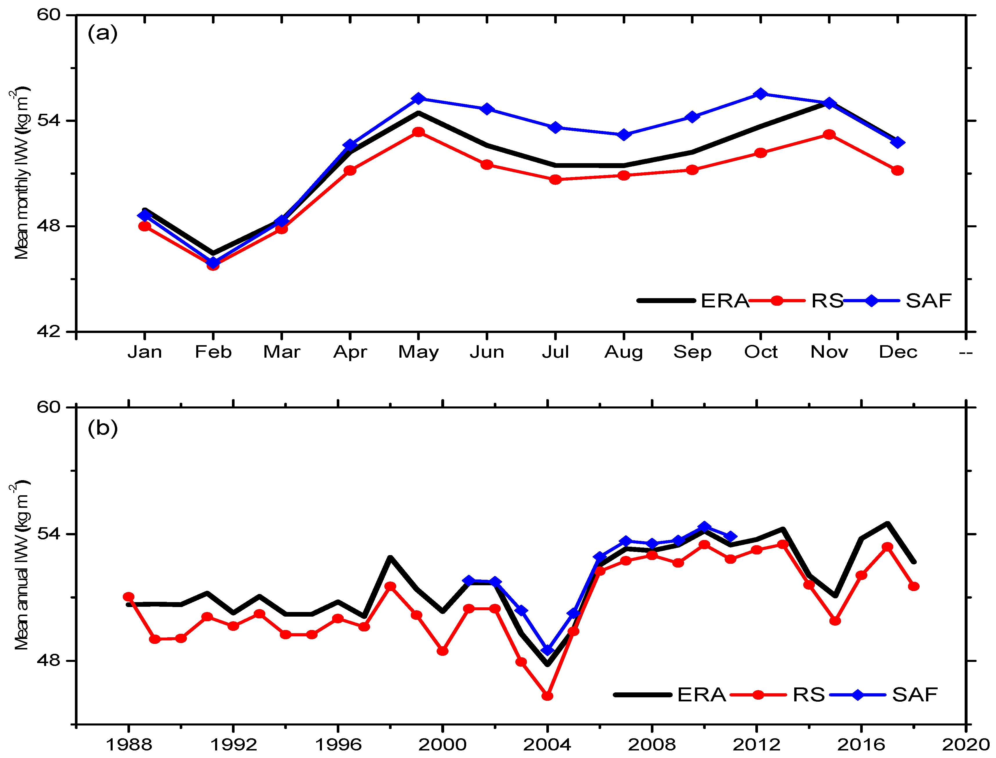
3.2.1. Temporal Variation

From Figure 4a in Section 3.1.2, which presents mean monthly cycle, it is obvious that IWV exhibits double oscillations, with pairs of minima and maxima for both datasets. ERA presents a primary minimum of 46.47 kgm−2 found in February. According to [29] and [55], this period is characterised by the lowest amount of rainfall in the peninsular, with a peak in November of each year. The amount of IWV engages a persistent increase from its lowest value in February until April and peaks in May, marking the secondary maximum throughout the region. The parameter dips slightly to its secondary minimum in August, coinciding with the second period of low precipitation as reported by [29]. The primary maximum is found in November, with the annual mean being 51.69 kgm−2. This value is consistent with the 51.28 kg m−2 reported by [56], who deployed GPS measurements between 2011 and 2014 to evaluate IWV in Peninsular Malaysia. Except for the different annual mean values of IWV presented by each of the datasets, their oscillations are fairly synchronous throughout (Figure 4b). Makama and Lim [25] reported similar cycles for RS and SAF when they compared IWV profiles from the two datasets for the same study location.
The primary maximum found in November, which also coincided with the second peak of precipitation, may be due to the retreat of the SWM and the equator-ward migration of the NEM wind, as can be seen in Figure 1b. The transition of these monsoons enhances the formation of a wide area of convergence that favours convection. Furthermore, the interactions between local topography and the prevailing north-easterly wind across the South China sea, from the abundant moisture squeezed into the region, may account for the high IWV at the onset of the NEM period. The primary minimum, observed in February, may indicate the retreat of the above prevailing circulations. Factors such as coastal upwelling and circulation aloft, which becomes divergent, and subsidence because of frequent occurrence of inversions and isothermals in the upper atmosphere [57], may be responsible for the dip in moisture at the retreat of the two monsoon seasons. It is worth noting that May and November are the respective beginnings of the SWM and the NEM seasons [58].

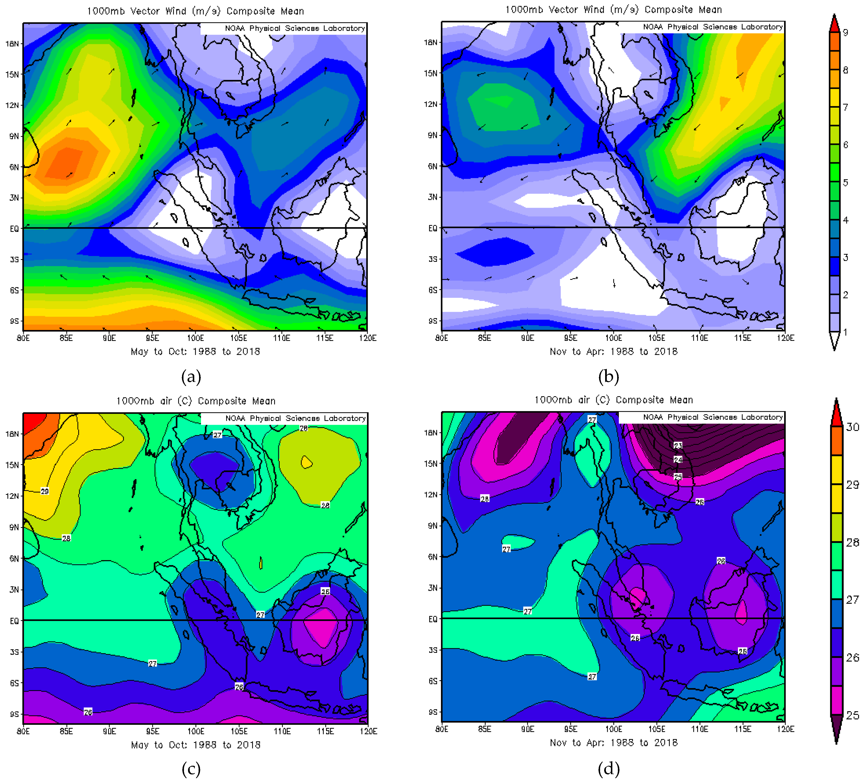
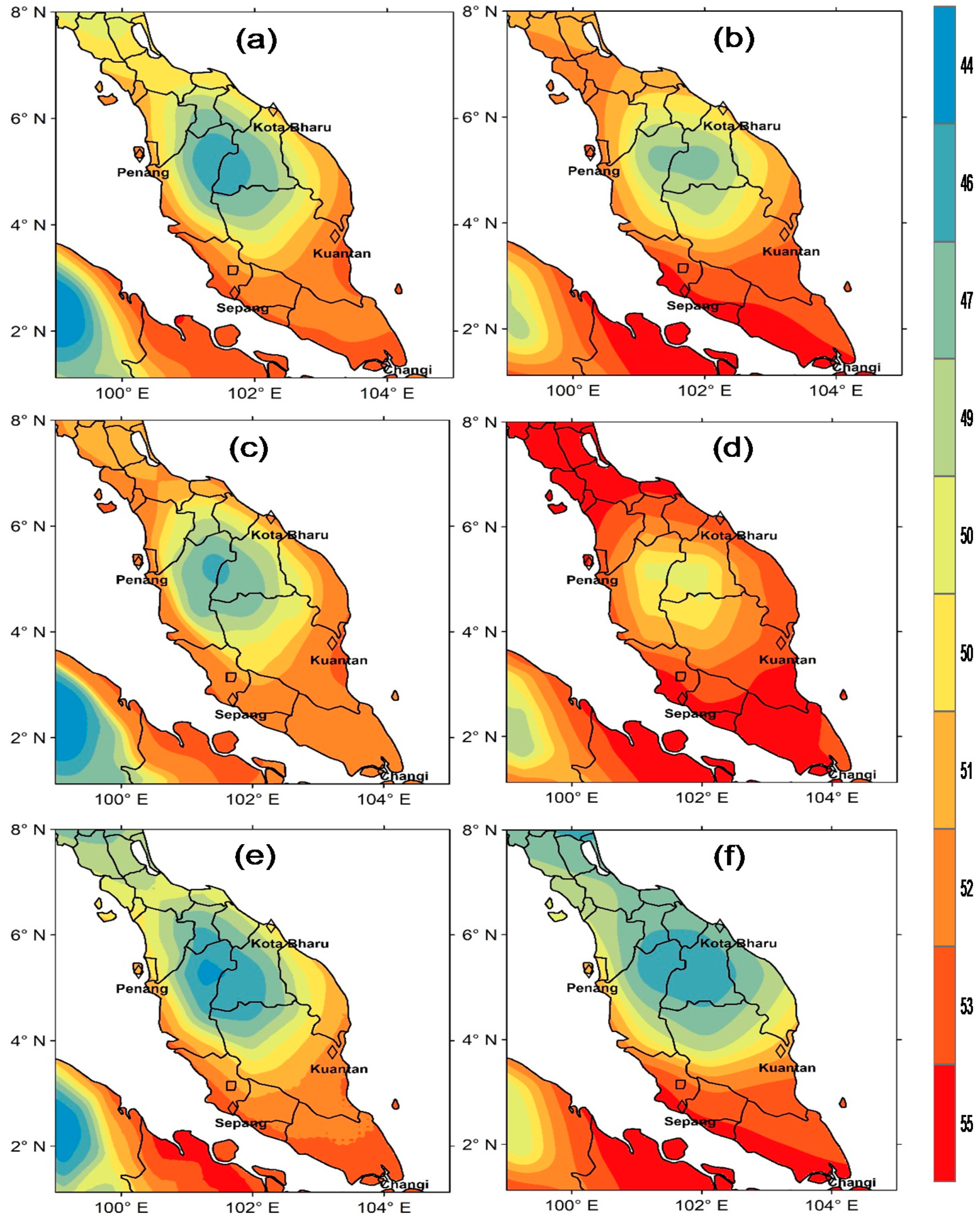
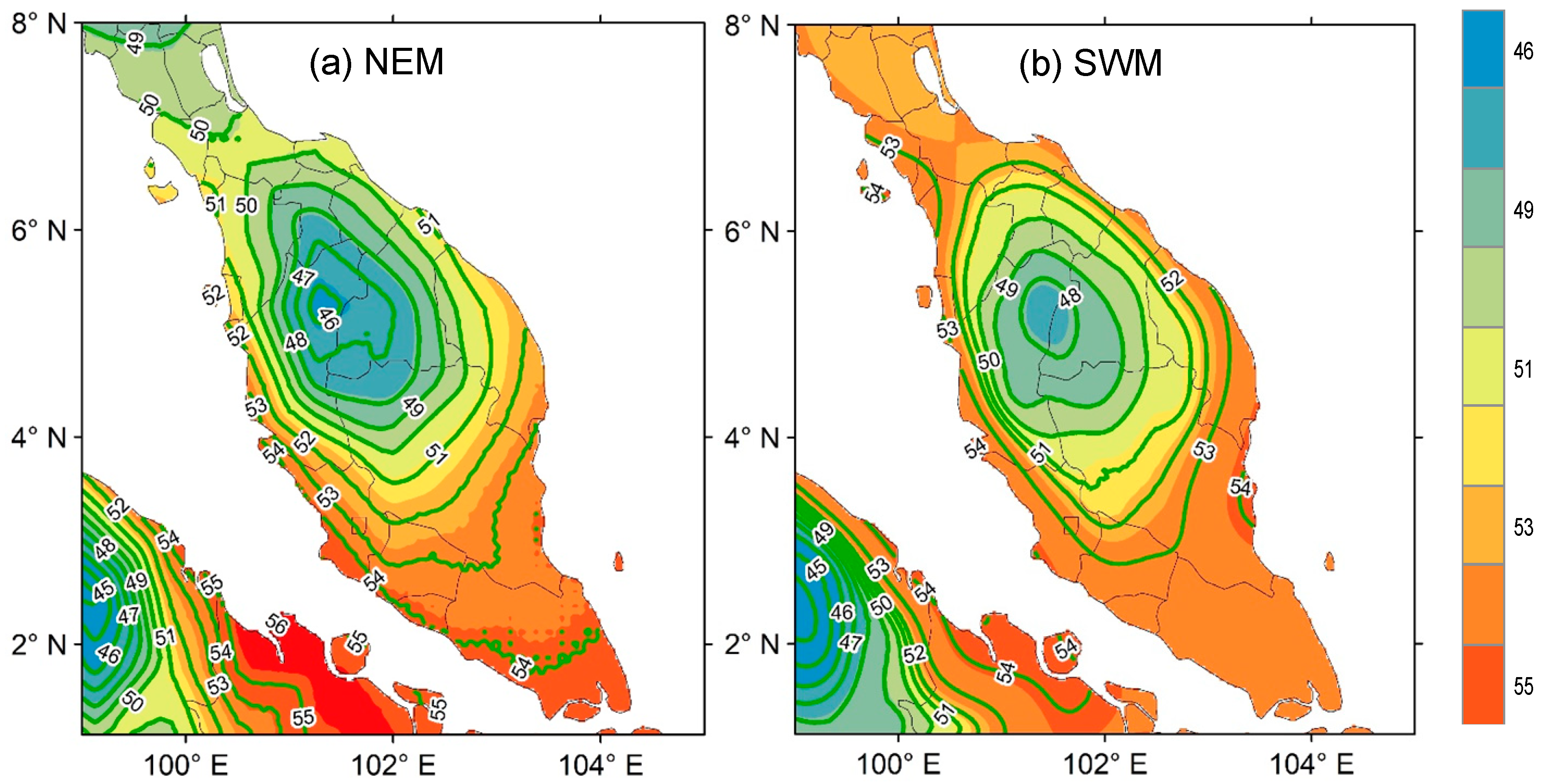
3.2.2. Spatial Variation

Figure 6 illustrates the spatial distribution maps of seasonal mean IWV from ERA IWV data for the NEM and SWM seasons during the 1988–2018 period. IWV decreases generally in a southeast–northwest orientation over Peninsular Malaysia, with the regional maximum appearing over the southeastern tip of the area in both seasonal distributions of the means. Complex and steep orography tends to shape the intense horizontal gradient along the edges of the peninsular. The rich horizontal gradients that manifest along the western boundary are relatively more intense in the SWM (Figure 6b) than the NEM (Figure 6a) and the annual (contours not shown) time scales. Weak horizontal gradients are easily noticed over the southern and central parts of the area in both seasons. Regional minima of IWV are, however, seen as they manifest local elevations, which is evidently noticed around the central regions (see Figure 1 inset). More water vapour is accounted for during the SWM than in the NEM, which is consistent with the seasonal cycle shown in Figure 4a.
The northward transport of water vapour, as can be seen in Figure 1a, may be responsible for the abundant water vapour with associated large horizontal gradients over the southeastern part of the peninsular during the SWM season. This water vapour transport is linked with the low-level monsoon flow and the steep topographic slopes of Titiwangsa mountains, which run from the Malaysia–Thailand border to the southern state of Negeri Sembilan (Figure 2 inset), blocking its farther northwestward intrusion. Generally, elevations are relatively lower to the south than towards the northern part, forming a southwest–northeast orientation of horizontal precipitable water gradients. It is, therefore, not surprising that areas with lower topography present higher IWV, since more moisture content tends to reside in the lower troposphere.
Within the peninsular, on the other hand, a relatively dry moisture regime tends to manifest high topography, as mentioned earlier. The seemingly dry IWV during the NEM season over areas like Kelantan and Terengganu, which are on the eastern coast of the peninsular, despite their higher rainfall amounts at this period [55], may be ascribed to higher topography that typifies the region. Moreover, during this season, the mean wind flow, controlled almost entirely by the northwesterlies that later transits into northeasterlies on reaching Peninsular Malaysia, as seen in Figure 1b, may be responsible for the apparent dry IWV in the region. On the other hand, relatively high IWV is observed in the northern parts of the peninsular during the SWM period, despite slower wind speed compared to the NEM wind [59,60]. This is because the SWM winds, which arrive at Peninsular Malaysia from the Indonesian Island of Sumatra (see Figure 1a), experience a moisture sheltering effect created by high mountain ranges [29]. Moreover, as the Strait of Malacca widens northwards, the land–sea breeze and convection exert local influence, to a large extent, on atmospheric moisture [61]. More so, the prevalently higher temperatures in the northern area, particularly during this period, as seen in Figure 1c, could induce evaporation rate and consequently, produce more moisture content aloft.

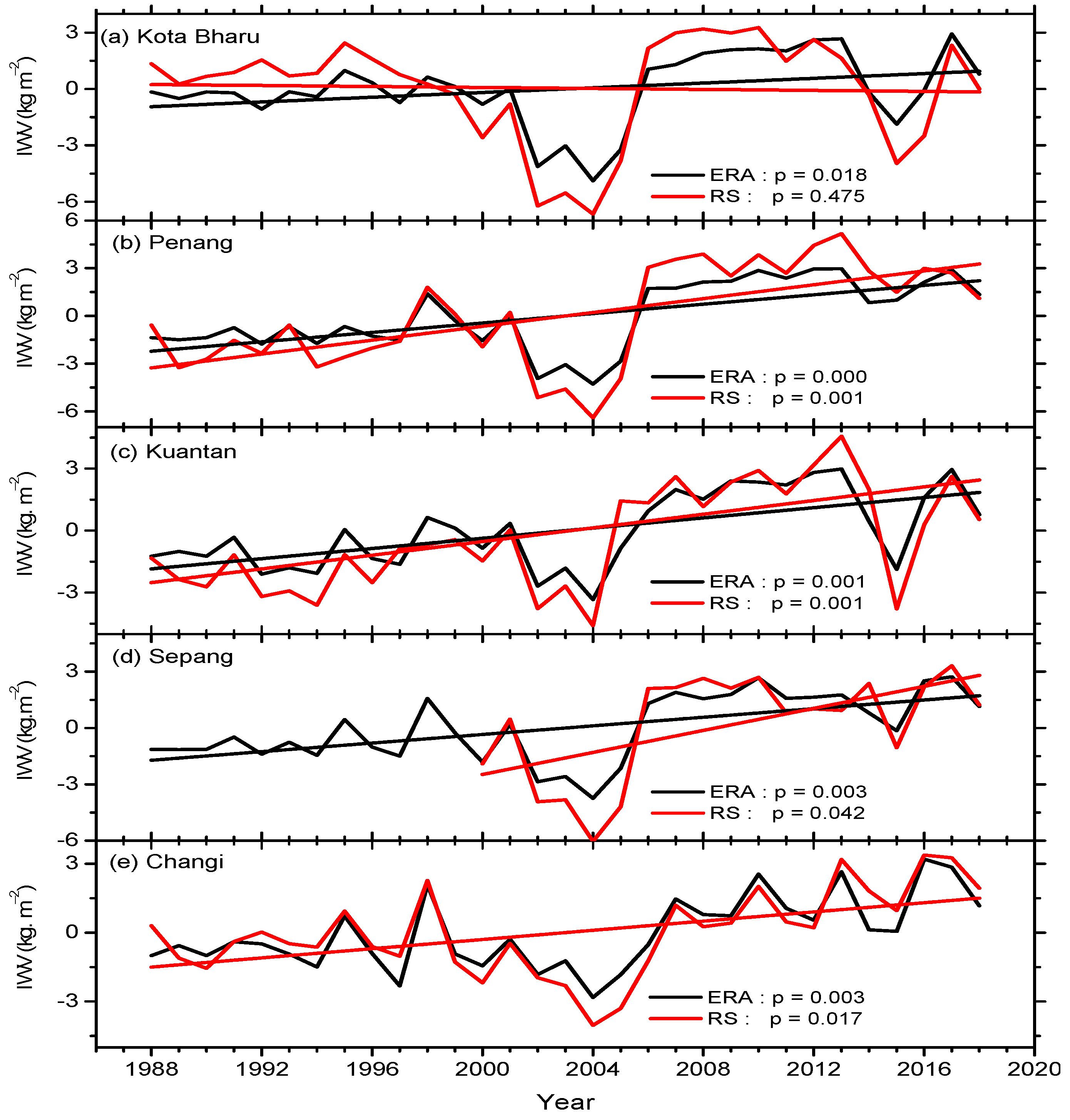
3.3. Long Term Trends in ERA and RS IWV (1988–2018)

Durre et al. [8] observed that for a better understanding of climate dynamics, it is important to investigate long-term trends in precipitable water vapour. Linear trends between 1988 and 2018 in monthly anomalies from ERA and RS IWVs are, therefore, performed for each station using the non-parametric M–K and T–S tests. The statistical significance of the trends and the T–S slope (β) for both annual and seasonal time scales are presented in Table 3, while the annual time series along with the corresponding p-values are depicted in Figure 7. Trends were also obtained in both the annual and seasonal time series for the entire region but are not shown. Due to the short temporal regime of SAF, it was not used for the long-term trend evaluation, as stated earlier. The IWV variational trends estimated from ERA over all the stations are positive and statistically significant at the 95% level and are consistent with the probability values shown in Figure 6, within the period under review. Highest and lowest trend rates of 0.15 ± 0.38 and 0.09 ± 0.34 kg m−2decade−1 are respectively recorded at Penang and Changi stations in the annual time series. Except for Kota Bharu, where a downward and nonsignificant trend of −0.03 ± 0.61 kg m−2decade−1 is found from the RS in the same period, trends elsewhere are positive and statistically significant. Respective highest and lowest trends of 0.21 ± 0.57 and 0.09 ± 0.43 kg m−2decade−1 are yet again found at Penang and Changi as is with the trends from ERA.
Trends from ERA for the annual time scale are also positive and statistically significant at all the stations during the NEM season, with the greatest and lowest rates of 0.20 ± 0.42 and 0.10 ± 0.34 kg m−2decade−1 found at Penang and Sepang, respectively. The RS similarly turned in increasing and significant trends in all the stations during this season, except at Kota Bharu and Sepang, where the trends were nonsignificant, though positive. The largest annual trend of 0.25 ± 0.61 kg m−2decade−1 from the RS is found in Penang during the NEM season. Increasing trends are also recorded in the SWM season from both ERA and RS in all the stations, except for the latter, whose trend is downward and nonsignificant at Kota Bharu. Other than the negative and positive trends respectively found at Kota Bharu from both ERA and RS during this season, the trends are statistically significant everywhere. The greatest trends from ERA and RS during the SWM are found in Kuantan and Penang, respectively. At the regional level, both ERA and RS present positive and statistically significant trends during the annual and seasonal time scales, except for the latter, whose trend is nonsignificant during the SWM period. Respective highest regional trends (not shown) from ERA and RS observations of 0.17 ± 0.34 and 0.14 ± 0.42 kg m−2decade−1, found in the NEM time scale, are consistent with the rates found at the individual stations.
From Figure 7, an abrupt drop in IWV is noticed in both ERA and RS between 2003 and 2004, with a steep climb in 2007 across the entire region. This sudden downward trend at all the stations from 2003 to 2004 and also at Kota Bharu, Kuantan, and Sepang in 2015, is most likely connected to the emergence of El Niño events [52], mentioned in Section 3.1.2. This event is mostly associated with warm and dry conditions that affect Malaysia and other adjoining areas. Saini and Gulati [62], in their report, attributed the Indian droughts of 2002 and 2004 to the El Niño events that occurred within these periods. Further analysis is, however, required to assess the impact of the different climatic events in the current area of study.
In general, both ERA and RS IWV show increasing trends that are statistically significant at both the regional and synoptic scales, as seen across most stations during the annual and seasonal time frames, with different intensities, though (see Figure 7). The observed proximity in IWV trends from the two sets of data is to be expected since the pair correlate excellently. However, a visual look at Figure 7 shows that RS trends are dominantly higher than those from ERA across the stations, particularly, from 2006 onwards, corroborating the finding of Chen and Liu [1]. In addition, from Table 3, the trends from RS are evidently higher than those of ERA in all the stations except at Kota Bharu, where statistically nonsignificant trends are obtained throughout. Overall, RS produced the highest trend, which occurred in Penang during the NEM season, while ERA produced the corresponding lowest value, obtained in Changi. The Z scores in Table 3 conform to the p-values (α = 0.05) depicted in Figure 6. Although seasonal upward trends are obtained across the stations during the two seasons, except for Kota Bharu in SWM, their relative magnitudes are not significantly different. Overall, the trends in IWV over Peninsular Malaysia between 1988 and 2018 are dominantly positive and relatively higher in the central and northern parts of the region than in the southern part, indicating marginally more moistening in the former over the years. The mainly upward IWV trends are consistent with the warming trends of 1.35–6.33 °C-Decade−1 in the past 50 years [63] and between 0.5 and 1.5 °C-Decade−1 in the past 30 years for Peninsular Malaysia [52].

4. Conclusions

Knowledge on the variability and long-term trends in integrated water vapour (IWV) over an area provides crucial information on weather and climatic changes, among others. In this study, monthly means of ERA-Interim reanalysis and radiosonde records, for the period 1988–2018, have been used to investigate the distribution and long-term trend of IWV over Peninsular Malaysia. Prior to trend analysis, ERA IWV was interpolated on radiosonde and CM-SAF datasets for performance evaluation. The main idea was to gauge the suitability of the ERA data for trend analysis in the study area. The means and variability in ERA IWV were, therefore, compared to RS, from 1988 to 2018 and SAF, from 2001 to 2011. The evaluation pointed to a dry average MB of −1.29 kg m−2 by RS relative to ERA, while SAF was wetter than ERA with a MB of 1.22 kg m−2, averaged over the five synoptic stations. These values are consistent with other studies e.g., [15,17]. The matching of ERA with SAF demonstrated relatively more accuracy than its comparison with RS based on the values of the RMS, which were 1.93 and 2.28 kg m−2 for the respective pairs of datasets, averaged over all the stations. The validation was more accurate in the northern stations compared to those at the southern fringe of the peninsular, which also had relatively lower R2 values. The seasonal time scale revealed uniform oscillations, with more moistening in most parts of the SWM than in the NEM. The interannual variability further revealed ERA’s high consistency with SAF and good agreement with RS, while maintaining its respective dry and wet biases against the two datasets. Based on the foregoing, it is safe to say that the ERA-Interim product is suitable for IWV studies in Peninsular Malaysia and was accordingly used to explore both its variability and trends.
The seasonal time scale of IWV in Peninsular Malaysia revealed double fluctuations with a pair of minima occurring in February and August, while maxima were found in May and November. The maxima occurred at the respective beginnings of the SWM and the NEM seasons, which are coincidental peaks in precipitation in the peninsular. The annual mean IWV of 51.69 kg m−2 is consistent with the 51.28 kg m−2 reported by Salihin et al. [55] for the same study area. The distribution of the monthly mean IWV throughout Peninsular Malaysia showed marked geographical and seasonal differences. The parameter was observed to decrease in a southeast–northwest orientation over the peninsular, with regional maximum appearing over the southeastern tip of the area in both seasonal distributions of the means. Complex and steep orography tended to shape intense horizontal gradient along the edges of the peninsular. The rich horizontal gradients that manifest along the western boundary were found to be relatively more intense in the SWM than in the NEM time scales. The spatial pattern also showed that more water vapour is found during the SWM than in the NEM season in Peninsular Malaysia.
Trend analysis was carried out using the non-parametric Mann–Kendall and Theil–Sen slope estimator tests. The trends in the interannual time series of the annual mean IWV in ERA were consistent with the observed RS series in Peninsular Malaysia. The largest and smallest values of IWV were found in 2017 and 2004, respectively. The sharp fall in IWV, noticed between 2003 and 2004 and 2015, coincided with El Niño events that occurred within the period [52]. Concerted analysis is, however, required to assess the impact of the different climatic events in the study area. Trends in ERA IWV at all the stations were positive and statistically significant at the 95% level in both the annual and seasonal time scales, except at Kota Bharu, where a nonsignificant trend was found during the SWM period. Though the trend from RS IWV for both time series were similarly positive everywhere, those at Kota Bharu in the annual and SWM time series were, however, negative and statistically insignificant just as the positive trends found there were. The greatest trend rate of 0.20 ± 0.42 kg m−2decade−1 was found at Penang in the NEM time series with the corresponding least value of 0.09 ± 0.28 kg m−2decade−1 found at Changi in the SWM series from ERA IWV. The RS IWV trend, on the other hand, returned the highest and lowest significant rates of 0.25 ± 0.61 and 0.11 ± 0.37 kg m−2decade−1 at Penang and Changi stations in the annual and NEM periods, respectively. IWV from both ERA and RS presented averagely higher trends in NEM and lowest in the SWM time series. The discrepancies found between ERA and RS trend values can be investigated further using the newly released ECMWF reanalysis product, ERA5. Overall, the IWV trend was mostly positive in Peninsular Malaysia, which is consistent with the global upward trends reported elsewhere e.g., [3,17,18,19,20].

Author Contributions

Conceptualisation, Funding Acquisition and Supervision, H.S.L.; Data Acquisition, Data Curation, Writing—Original Draft Preparation, Formal Analysis, and Visualisation, E.K.M. All authors have read and agreed to the published version of the manuscript.

Funding

This research was funded by RUI grant (Burning in Southeast Asia Maritime Continent), 1001/PFIZIK/8011079.

Acknowledgments

The authors would like to acknowledge the European Centre for Medium-Range Weather Forecasts (ECMWF) for providing the reanalysis data (https://www.ecmwf.int/), the National Oceanic and Atmospheric Administration (NOAA) for the IGRA2 data (www.ncdc.noaa.gov/data-access/weather-balloon/integrated-global-radiosonde-archive), and the Satellite Application Facility on Climate Monitoring (CM-SAF) of European Organization for the Exploitation of Meteorological Satellites (EUMETSAT) for the ATOVS-derived Climate Data Records provided (https://wui.cmsaf.eu).

Conflicts of Interest

The authors declare no conflict of interest. The funders had no role in the design of the study, in the collection, analyses, or interpretation of data, in the writing of the manuscript, or in the decision to publish the results.

References

  1. Wagner, T.; Beirle, S.; Grzegorski, M.; Platt, U. Global trends (1996–2003) of total column precipitable water observed by Global Ozone Monitoring Experiment (GOME) on ERS-2 and their relation to near-surface temperature. J. Geophys. Res. 2006, 111, D12102. [Google Scholar] [CrossRef] [Green Version]
  2. Dai, A.; Wang, J.; Thorne, P.W.; Parker, D.E.; Haimberger, L.; Wang, X.L. A New Approach to Homogenize Daily Radiosonde Humidity Data. J. Clim. 2011, 24, 965–991. [Google Scholar] [CrossRef]
  3. Trenberth, K.E.; Fasullo, J.; Smith, L. Trends and variability in column-integrated atmospheric water vapor. Clim. Dyn. 2005, 24, 741–758. [Google Scholar] [CrossRef]
  4. Trenberth, K.E. Atmospheric moisture residence times and cycling: Implications for rainfall rates and climate change. Clim. Chang. 1998, 39, 667–694. [Google Scholar] [CrossRef]
  5. Alshawaf, F.; Balidakis, K.; Dick, G.; Heise, S.; Wickert, J. Estimating trends in atmospheric water vapor and temperature time series over Germany. Atmos. Meas. Tech. 2017, 10, 3117–3132. [Google Scholar] [CrossRef] [Green Version]
  6. Tuller, S.E. The relationship between precipitable water vapor and surface humidity in New Zealand. Mon. Weather Rev. 1977, 26, 197–212. [Google Scholar] [CrossRef]
  7. Peng, W.; Tongchuan, X.; Jiageng, D.; Jingmin, S.; Yanling, W.; Qingli, S.; Xin, D.; Hongliang, Y.; Dejun, S.; Jinrong, Z. Trends and Variability in Precipitable Water Vapor throughout North China from 1979 to 2015. Adv. Meteorol. 2017, 2017, 1–10. [Google Scholar] [CrossRef] [Green Version]
  8. Wang, J.; Dai, A.; Mears, C. Global Water Vapor Trend from 1988 to 2011 and Its Diurnal Asymmetry Based on GPS, Radiosonde, and Microwave Satellite Measurements. J. Clim. 2016, 29, 5205–5222. [Google Scholar] [CrossRef]
  9. Durre, I.; Williams, C.N.; Yin, X.; Vose, R.S. Radiosonde-based trends in precipitable water over the Northern Hemisphere: An update. J. Geophys. Res. Atmos. 2009, 114, 1–8. [Google Scholar] [CrossRef]
  10. Xu, G.; Ware, R.S.; Zhang, W.; Feng, G.; Liao, K.; Liu, Y. Effect of off-zenith observations on reducing the impact of precipitation on ground-based microwave radiometer measurement accuracy. Atmos. Res. 2014, 140–141, 85–94. [Google Scholar] [CrossRef]
  11. Opaluwa, Y.D.; Norazmi, M.F.; Musa, T.A.; Othman, R.; Eyo, E. Trend in ground-based GPS sensing of atmospheric water vapour: The Malaysian perspective. J. Teknol. 2014, 71, 35–47. [Google Scholar] [CrossRef] [Green Version]
  12. Bevis, M.; Businger, S.; Herring, T.A.; Rocken, C.; Anthes, R.A.; Ware, R.H. GPS meteorology: Remote sensing of atmospheric water vapor using the global positioning system. J. Geophys. Res. 1992, 97, 15787. [Google Scholar] [CrossRef]
  13. Wang, Y.; Tang, L.; Zhang, J.; Gao, T.; Wang, Q.; Song, Y.; Hua, D. Investigation of Precipitable Water Vapor Obtained by Raman Lidar and Comprehensive Analyses with Meteorological Parameters in Xi’an. Remote Sens. 2018, 10, 967. [Google Scholar] [CrossRef] [Green Version]
  14. Schröder, M.; Jonas, M.; Lindau, R.; Schulz, J.; Fennig, K. The CM SAF SSM/I-based total column water vapour climate data record: Methods and evaluation against re-analyses and satellite. Atmos. Meas. Tech. 2013, 6, 765–775. [Google Scholar] [CrossRef] [Green Version]
  15. Liu, Z.; Wong, M.S.; Nichol, J.; Chan, P.W. A multi-sensor study of water vapour from radiosonde, MODIS and AERONET: A case study of Hong Kong. Int. J. Climatol. 2013, 33, 109–120. [Google Scholar] [CrossRef] [Green Version]
  16. Chen, B.; Liu, Z. Global water vapor variability and trend from the latest 36 year (1979 to 2014) data of ECMWF and NCEP reanalyses, radiosonde, GPS, and microwave satellite. J. Geophys. Res. Atmos. 2016, 121, 11442–11462. [Google Scholar] [CrossRef]
  17. Ross, R.J.; Elliott, W.P. Tropospheric Water Vapor Climatology and Trends over North America: 1973–93. J. Clim. 1996, 9, 3561–3574. [Google Scholar] [CrossRef] [Green Version]
  18. Parracho, A.C.; Bock, O.; Bastin, S. Global IWV trends and variability in atmospheric reanalyses and GPS observations. Atmos. Chem. Phys. 2018, 18, 16213–16237. [Google Scholar] [CrossRef] [Green Version]
  19. Xie, B.; Zhang, Q.; Ying, Y. Trends in Precipitable Water and Relative Humidity in China: 1979–2005. J. Appl. Meteorol. Climatol. 2011, 50, 1985–1994. [Google Scholar] [CrossRef]
  20. Arguez, A.; Vose, R.S. The definition of the standard WMO climate normal: The key to deriving alternative climate normals. Bull. Am. Meteorol. Soc. 2011, 92, 699–704. [Google Scholar] [CrossRef]
  21. Alshawaf, F.; Hinz, S.; Mayer, M.; Meyer, F.J. Constructing accurate maps of atmospheric water vapor by combining interferometric synthetic aperture radar and GNSS observations. J. Geophys. Res. Atmos. 2015, 120, 1391–1403. [Google Scholar] [CrossRef]
  22. Uppala, S.M.; KÅllberg, P.W.; Simmons, A.J.; Andrae, U.; Bechtold, V.D.C.; Fiorino, M.; Gibson, J.K.; Haseler, J.; Hernandez, A.; Kelly, G.A.; et al. The ERA-40 re-analysis. Q. J. R. Meteorol. Soc. 2005, 131, 2961–3012. [Google Scholar] [CrossRef]
  23. Zhang, Y.; Wang, D.; Zhai, P.; Gu, G.; He, J. Spatial Distributions and Seasonal Variations of Tropospheric Water Vapor Content over the Tibetan Plateau. J. Clim. 2013, 26, 5637–5654. [Google Scholar] [CrossRef]
  24. Makama, E.K.; Lim, H.S. Characteristics of precipitable water over Peninsular Malaysia from satellite and in situ data. Terr. Atmos. Ocean. Sci. 2017, 28, 979–992. [Google Scholar] [CrossRef] [Green Version]
  25. Peng, G.; Li, J.; Chen, Y.; Norizan, A.P.; Tay, L. High-resolution surface relative humidity computation using MODIS image in Peninsular Malaysia. Chinese Geogr. Sci. 2006, 16, 260–264. [Google Scholar] [CrossRef]
  26. Amirabadizadeh, M.; Huang, Y.F.; Lee, T.S. Recent Trends in Temperature and Precipitation in the Langat River Basin, Malaysia. Adv. Meteorol. 2015, 2015, 1–16. [Google Scholar] [CrossRef] [Green Version]
  27. Mahmud, M.R.; Numata, S.; Matsuyama, H.; Hosaka, T.; Hashim, M. Assessment of effective seasonal downscaling of TRMM precipitation data in Peninsular Malaysia. Remote Sens. 2015, 7, 4092–4111. [Google Scholar] [CrossRef] [Green Version]
  28. Wong, C.L.; Venneker, R.; Uhlenbrook, S.; Jamil, A.B.M.; Zhou, Y. Variability of rainfall in Peninsular Malaysia. Hydrol. Earth Syst. Sci. Discuss. 2009, 6, 5471–5503. [Google Scholar] [CrossRef] [Green Version]
  29. Dee, D.P.; Uppala, S.M.; Simmons, A.J.; Berrisford, P.; Poli, P.; Kobayashi, S.; Andrae, U.; Balmaseda, M.A.; Balsamo, G.; Bauer, P.; et al. The ERA-Interim reanalysis: Configuration and performance of the data assimilation system. Q. J. R. Meteorol. Soc. 2011, 137, 553–597. [Google Scholar] [CrossRef]
  30. Ccoica-López, K.; Pasapera-Gonzales, J.; Jimenez, J. Spatio-Temporal Variability of the Precipitable Water Vapor over Peru through MODIS and ERA-Interim Time Series. Atmosphere 2019, 10, 192. [Google Scholar] [CrossRef] [Green Version]
  31. National Centers for Environmental Information Home Page. Available online: https://www.ncdc.noaa.gov/data-access/weather-balloon/integrated-global-radiosonde-archive (accessed on 10 June 2020).
  32. Mattar, C.; Sobrino, J.A.; Julien, Y.; Morales, L. Trends in column integrated water vapour over Europe from 1973 to 2003. Int. J. Climatol. 2011, 31, 1749–1757. [Google Scholar] [CrossRef]
  33. Adeyemi, B.; Joerg, S. Analysis of water vapor over Nigeria using radiosonde and satellite data. J. Appl. Meteorol. Climatol. 2012, 51, 1855–1866. [Google Scholar] [CrossRef]
  34. Li, J.; Wolf, W.W.; Menzel, W.P.; Zhang, W.; Huang, H.-L.; Achtor, T.H. Global Soundings of the Atmosphere from ATOVS Measurements: The Algorithm and Validation. J. Appl. Meteorol. 2000, 39, 1248–1268. [Google Scholar] [CrossRef]
  35. Europian Meteorological Satellite (EUMETSAT): Satellite Application for Climate Monitoring (CM SAF) Home Page. Available online: http://www.cmsaf.eu/wui (accessed on 4 June 2020).
  36. European Centre for Medium-Range Weather Forecasts (ECMWF):|Advancing Global Numerical Weather Prediction (NWP) through International Collaboration. Available online: https://www.ecmwf.int/en/forecasts/datasets/reanalysis-datasets/era-interim (accessed on 3 June 2020).
  37. Ning, T.; Wickert, J.; Deng, Z.; Heise, S.; Dick, G.; Vey, S.; Schöne, T. Homogenized Time Series of the Atmospheric Water Vapor Content Obtained from the GNSS Reprocessed Data. J. Clim. 2016, 29, 2443–2456. [Google Scholar] [CrossRef]
  38. Khambhammettu, P. Annual Groundwater Monitoring Report: Mann-Kendall Analysis for the Ford Ord Site; HydroGeologic, Inc: Reston, VA, USA, 2004. [Google Scholar]
  39. Theil, H. A Rank-Invariant Method of Linear and Polynomial Regression Analysis, I, II, III. Nederl. Akad. Wetensch. 1950, 53, 386–392, 521–525, 1397–1412. [Google Scholar]
  40. Sen, P.K. Estimates of the Regression Coefficient Based on Kendall’s Tau. J. Am. Stat. Assoc. 1968, 63, 1379–1389. [Google Scholar] [CrossRef]
  41. Gocic, M.; Trajkovic, S. Analysis of changes in meteorological variables using Mann-Kendall and Sen’ s slope estimator statistical tests in Serbia. Glob. Planet. Chang. 2013, 100, 172–182. [Google Scholar] [CrossRef]
  42. Soden, B.J.; Lanzante, J.R. An assessment of satellite and radiosonde climatologies of upper-tropospheric water vapor. J. Clim. 1996, 9, 1235–1250. [Google Scholar] [CrossRef]
  43. Courcoux, N.; Schröder, M. The CM SAF ATOVS tropospheric water vapour and temperature data record: Overview of methodology and evaluation. Earth Syst. Sci. Data Discuss. 2015, 127–171. [Google Scholar] [CrossRef]
  44. Wang, J.; Zhang, L. Systematic Errors in Global Radiosonde Precipitable Water Data from Comparisons with Ground-Based GPS Measurements. J. Clim. 2008, 21, 2218–2238. [Google Scholar] [CrossRef]
  45. Waller, J.A.; Dance, S.L.; Lawless, A.S.; Nichols, N.K.; Eyre, J.R. Representativity error for temperature and humidity using the Met Office high-resolution model. Q. J. R. Meteorol. Soc. 2014, 140, 1189–1197. [Google Scholar] [CrossRef]
  46. Miloshevich, L.M.; Paukkunen, A.; Vömel, H.; Oltmans, S.J. Development and Validation of a Time-Lag Correction for Vaisala Radiosonde Humidity Measurements. J. Atmos. Ocean. Technol. 2004, 21, 1305–1327. [Google Scholar] [CrossRef]
  47. Liu, Y.; Tang, N. Humidity sensor failure: A problem that should not be neglected. Atmos. Meas. Tech. 2014, 7, 3909–3916. [Google Scholar] [CrossRef] [Green Version]
  48. Li, Z. Comparison of precipitable water vapor derived from radiosonde, GPS, and Moderate-Resolution Imaging Spectroradiometer measurements. J. Geophys. Res. 2003, 108, 4651. [Google Scholar] [CrossRef]
  49. Balogun, E.E.; Adedokun, J.A. On the Variations in Precipitable Water over Some West African Stations during the Special Observation Period of WAMEX. Mon. Weather Rev. 1986, 114, 772–776. [Google Scholar] [CrossRef] [Green Version]
  50. Peixoto, J.P.; Oort, A.H. Climatology of relative humidity. Am. Meteorol. Soc. 1996, 9, 3443–3463. [Google Scholar]
  51. Varikoden, H.; Preethi, B.; Samah, A.A.; Babu, C.A. Seasonal variation of rainfall characteristics in different intensity classes over Peninsular Malaysia. J. Hydrol. 2011, 404, 99–108. [Google Scholar] [CrossRef]
  52. Vyas Pandey, A.K.; Misra, S.B.Y. Climate Change and Agriculture in India: Impact and Adaptation; Sheraz Mahdi, S., Ed.; Springer International Publishing: Cham, Switzerland, 2019; ISBN 978-3-319-90085-8. [Google Scholar]
  53. MMD. Climate Change Scenarios for Malaysia 2001–2099; Malaysian Meteorological Department, Ministry of Science, Technology and Innovation: Kuala Lumpur, Malaysia, 2009. [Google Scholar]
  54. Seemann, S.W.; Borbas, E.E.; Knuteson, R.O.; Stephenson, G.R.; Huang, H.L. Development of a global infrared land surface emissivity database for application to clear sky sounding retrievals from multispectral satellite radiance measurements. J. Appl. Meteorol. Climatol. 2008, 47, 108–123. [Google Scholar] [CrossRef]
  55. Camerlengo, A.; Somchit, N. Monthly and Annual Rainfall Variability in Peninsular Malaysia. Pertanika J. Sci. Technol. 2000, 8, 73–83. [Google Scholar]
  56. Salihin, S.; Musa, T.A.; Radzi, Z.M. Spatio-temporal estimation of integrated water vapour over the Malaysian peninsula during monsoon season. In Proceedings of the International Archives of the Photogrammetry, Remote Sensing and Spatial Information Sciences-ISPRS Archives, Kuala Lumpur, Malaysia, 4 October 2017; Volume 42, pp. 165–175. [Google Scholar]
  57. Willoughby, A.A.; Aro, T.O.; Owolabi, I.E. Seasonal variations of radio refractivity gradients in Nigeria. J. Atmos. Solar-Terrestrial Phys. 2002, 64, 417–425. [Google Scholar] [CrossRef]
  58. Camerlengo, A.L.; Demmler, M.I. Wind-driven circulation of Peninsular Malaysia’s Eastern continental shelf. Sci. Mar. 1997, 61, 203–211. [Google Scholar]
  59. Suhaila, J.; Jemain, A.A. Investigating the impacts of adjoining wet days on the distribution of daily rainfall amounts in Peninsular Malaysia. J. Hydrol. 2009, 368, 17–25. [Google Scholar] [CrossRef]
  60. Tangang, F.T. Low frequency and quasi-biennial oscillations in the Malaysian precipitation anomaly. Int. J. Climatol. 2001, 21, 1199–1210. [Google Scholar] [CrossRef]
  61. Oki, T.; Musiake, K. Seasonal Change of the Diurnal Cycle of Precipitation over Japan and Malaysia. J. Appl. Meteorol. 1994, 33, 1445–1463. [Google Scholar] [CrossRef] [Green Version]
  62. Saini, S.; Gulati, A. El Niño and Indian Droughts-A Scoping Exercise, Working Paper; Indian Council for Research on International Economic Relations: New Delhi, India, 2014. [Google Scholar]
  63. Ng Meng, W.; Alejandro, C.; Abdul Wahab, A. A Study Of Global Warming In Malaysia. J. Teknol. F 2005, 42, 1–10. [Google Scholar]
Figure 1. Distribution of mean wind speed (m/s) and direction (upper row) and mean temperature in °C (lower row) for the southwest monsoon (SWM) (a,c) and the northeast monsoon (b,d) over Peninsular Malaysia from 1988 to 2018.
Atmosphere 11 01012 g001
Figure 2. Peninsular Malaysia showing integrated global radiosonde archives (IGRA) stations (filled diamond), from which integrated precipitable water vapour (IWV) data were obtained. Inset is the topographic map of the study area.
Atmosphere 11 01012 g002
Figure 3. Scatterplots of monthly means of IWV from ERA compared with IWV from: Radiosonde ((left) panel) and CM-SAF ((right) panel) for the five selected WMO stations in Peninsular Malaysia.
Atmosphere 11 01012 g003
Figure 4. (a) Seasonal cycle of monthly mean and (b) Annual mean time series of IWV over Peninsular Malaysia for ERA-Interim (1988–2018), radiosonde (1988–2018), and CM-SAF (2001–2011) observations.
Atmosphere 11 01012 g004
Figure 5. Comparison of the spatial evolution of integrated water vapour (IWV) between (a,c,e): ERA-Interim (1988–2018) and (b,d,f): CM-SAF (2001–2011). The first row is for mean annual values, while the second and third rows are for SWM and NEM, respectively.
Atmosphere 11 01012 g005
Figure 6. Seasonal-mean ERA-Interim IWV for (a) NEM (November–April) and (b) SWM (May–October) for the 31-year (1988–2018) period over Peninsular Malaysia. Contours, in kg m−2, are also shown.
Atmosphere 11 01012 g006
Figure 7. Domain mean of monthly anomalies in annual time series from ERA-Interim IWV (black) interpolated to the nearest station location of the radiosonde IWV (red) with the associated probabilities (p) at 95% confidence interval for the five in situ stations (see Figure 1).
Atmosphere 11 01012 g007
Table 1. Description of the datasets and their sources.
Data/SourceStudy Area/LocationInstrumentTemporal/
Spatial Resolution
Temporal Coverage
NameLongitude (Degree)Latitude (Degree)
Radiosonde/IGRAKota Bharu102.2836.167Vaisala (RS80)
Vaisala (RS 92G)
Twice daily observations
(00 and 12 UTC)
1988–1993
1994–2018
Penang100.2675.300Vaisala (RS80)
Vaisala (RS 92G)
1988–1993
1993–2018
Kuantan103.2173.783Vaisala (RS80)
Vaisala (RS 92G)
1988–1993
1994–2018
Sepang
Changi
101.700
103.983
2.717
1.367
Graw DMF09
Vaisala (RS80)
Vaisala (RS 92G)
2000–2019
1988–1994
1994–2018
ERA-Interim Reanalysis/ECMWFPeninsular Malaysia97–106° E1–7° NNWP6–hourly observations/
79 × 79 km2
1988–2018
ATOVS/CM-SAFPeninsular Malaysia97–106° E1–7° NATOVSDaily observations/
90 × 90 km2
2001–2011
Table 2. Statistical proximity between IWV (Integrated water vapour) from ERA (1988–2018) when compared to RS (1988–2018) and SAF (2001–2011) IWV observations in Peninsular Malaysia. n is number of observations.
StationRS/ERASAF/ERA
nMB
(kgm−2)
RMS
(kgm−2)
nMB
(kgm−2)
RMS
(kgm−2)
Kota Bharu360−0.402.041320.871.91
Penang372−0.301.501321.331.87
Kuantan336−0.771.721320.631.42
Sepang228−1.062.091321.942.01
Changi372−2.854.051321.342.43
Table 3. Decadal trend estimates in ERA-Interim and Radiosonde IWV over five synoptic stations for the annual, northeast monsoon (NEM) and southwest monsoon (SWM) time scales (Unit: kgm−2 Decade−1). Z scores and trend direction are also given.
PeriodStationERA-InterimRadiosonde
Test
Score
(Z)
β
(kgm−2 decade−1)
Trend
(At 95% sig. Level)
Test Score
(Z)
β
(kgm−2 decade−1)
Trend
(At 95%
sig. Level)
AnnualKota Bharu2.360.09 ± 0.65Positive−0.75−0.03 ± 0.61 *Negative
Penang3.520.15 ± 0.38Positive3.230.21 ± 0.57Positive
Kuantan3.380.14 ± 0.33Positive3.470.20 ± 0.44Positive
Sepang2.980.10 ± 0.38Positive2.030.19 ± 0.68Positive
Changi2.960.09 ± 0.34Positive2.380.09 ± 0.43Positive
NEMKota Bharu2.070.13 ± 0.42Positive0.220.02 ± 0.65 *Positive
Penang4.010.20 ± 0.42Positive3.510.25 ± 0.61Positive
Kuantan3.230.16 ± 0.38Positive3.420.20 ± 0.46Positive
Sepang3.600.10 ± 0.34Positive1.400.06 ± 0.63 *Positive
Changi2.050.10 ± 0.38Positive2.670.10 ± 0.40Positive
SWMKota Bharu1.170.04 ± 0.37 *Positive−1.43−0.08 ± 0.69 *Negative
Penang2.470.11 ± 0.39Positive2.890.19 ± 0.56Positive
Kuantan2.640.12 ± 0.34Positive3.060.18 ± 0.48Positive
Sepang2.390.09 ± 0.36Positive2.400.11 ± 0.75Positive
Changi2.330.09 ± 0.28Positive2.890.11 ± 0.37Positive
* Nonsignificant trend.

