Evaluation of the Four-Dimensional Ensemble-Variational Hybrid Data Assimilation with Self-Consistent Regional Background Error Covariance for Improved Hurricane Intensity Forecasts

Abstract

The feasibility of a hurricane initialization framework based on the Gridpoint Statistical Interpolation (GSI)-based four-dimensional ensemble-variational (GSI-4DEnVar) hybrid data assimilation system for the Hurricane Weather Research and Forecasting model (HWRF) model is evaluated in this study. The system considers the temporal evolution of error covariances via the use of four-dimensional ensemble perturbations that are provided by high-resolution, self-consistent HWRF ensemble forecasts. It is different from the configuration of the GSI-based three-dimensional ensemble-variational (GSI-3DEnVar) hybrid data assimilation system, similar to that used in the operational HWRF, which employs background error covariances provided by coarser-resolution global ensembles from the National Centers for Environmental Prediction (NCEP) Global Forecast System (GFS) ensemble Kalman filtering data assimilation system. In addition, our proposed initialization framework discards the empirical intensity correction in the vortex initialization package that is employed by the GSI-3DEnVar initialization framework in operational HWRF. Data assimilation and numerical simulation experiments for Hurricanes Joaquin (2015), Patricia (2015), and Matthew (2016) are conducted during their intensity changes. The impacts of two initialization frameworks on the HWRF analyses and forecasts are compared. It is found that GSI-4DEnVar leads to a reduction in track, minimum sea level pressure (MSLP), and maximum surface wind (MSW) forecast errors in all of the HWRF simulations, compared with the GSI-3DEnVar initialization framework. With assimilating high-resolution observations within the hurricane inner-core region, GSI-4DEnVar can produce the initial hurricane intensity reasonably well without the empirical vortex intensity correction. Further diagnoses with Hurricane Joaquin indicate that GSI-4DEnVar can significantly alleviate the imbalances in the initial conditions and enhance the performance of the data assimilation and subsequent hurricane intensity and precipitation forecasts.

1. Introduction

The intensity forecasts for tropical cyclones (TCs) are of great importance for providing earlier warnings of TC-related damages [1,2]. However, accurate intensity forecasts, especially during TC intensity changes, remain a great challenge in the current operational and research community [3,4,5,6,7]. For instance, the official 48-h intensity forecast error only decreased by about 5–10% between 2000 and 2016 [8]. Part of the difficulty in improving intensity forecasts of TCs originates from uncertainties in the initial conditions provided for TC forecasting models [4,9]. At the U. S. National Centers for Environmental Prediction (NCEP), the Hurricane Weather Research and Forecasting (HWRF) model [10] has operationally provided real-time TC forecasts to the National Hurricane Center (NHC) for the Atlantic and eastern North Pacific basins since 2007 and was extended to all oceanic basins over the globe in 2014. The operational HWRF initialization adopts a vortex initialization (VI) package [11] and a Gridpoint Statistical Interpolation (GSI)-based three-dimensional ensemble-variational (3DEnVar) hybrid data assimilation (DA) system [12,13]. The VI package is based on a dynamical initialization scheme that first relocates the vortex to its observed location, followed by a size and intensity correction process with adjustments to the wind, moisture, and thermodynamics fields [14]. After that, DA is performed to incorporate the available conventional, radar, and satellite data into the first guess from VI with GSI-3DEnVar, where the flow-dependent background error covariance is derived from a set of Global Forecast System (GFS) ensemble Kalman filtering (EnKF) ensemble forecasts [14]. This further improves the vortex structure and environmental conditions for HWRF TC forecasts. The combination of VI and the GSI-3DEnVar DA system has substantially contributed to improvements in the track and intensity forecasts of HWRF, including those during changes in TC intensity [10].

Despite the significant progress in improving NCEP operational hurricane forecasts with the HWRF model and its data assimilation system, problems associated with the VI and DA system in HWRF have also been reported in recent studies. First, the VI in HWRF can lead to an unrealistic initial vortex inner-core structure [4] and vortex spin-down problems (e.g., a drop of 10∼20 knots in the maximum surface wind in the first few hours of a forecast) in HWRF [9] in some cases. Second, the VI and DA in HWRF have been shown to counteract each other in some cases [15]. Third, the current GSI-3DEnVar system does not account for the temporal evolution of error covariance within the assimilation window [16], and the resolution of the GFS ensemble covariance is too coarse to properly resolve the error covariance of the TC inner core [9,14]. Due to these deficiencies, in some cases the initial conditions for HWRF are suboptimal, leading to the degradation of track and intensity forecasts, especially during changes in TC intensity [17]. Thus, resolving these problems is essential in order to further improve the forecasts of TC intensity changes in HWRF. Recent studies have explored ways to overcome these problems. Ref. [9] used high-resolution, self-consistent regional HWRF ensembles instead of a global ensemble to derive the flow-dependent background error covariances in GSI-3DEnVar for HWRF, resulting in a more realistic hurricane initial inner-core structure and leading to improved hurricane forecasting. In addition, the GSI-based four-dimensional ensemble-variational hybrid DA system (GSI-4DEnVar) has been developed for operational TC forecast models [14,16,18]. In GSI-4DEnVar, ensemble perturbations at multiple time periods spanning the assimilation window are used to incorporate the temporal evolution of the background error covariances into the DA system. Moreover, GSI-4DEnVar is computationally cheap relative to the traditional 4DVar DA system because it avoids using the tangent linear model and adjoint model [16,18]. Studies have shown that GSI-4DEnVar outperforms GSI-3DEnVar in producing more realistic TC analyses and can further improve TC intensity forecasts [14,16,18]. More importantly, recent studies have found that the assimilation of high-resolution inner-core observations (e.g., High-Definition Sounding System dropsonde data) based on the GSI-4DEnVar with a high-resolution background error covariance can outperform the VI scheme currently used in HWRF [19].

In light of these recent developments, this study assesses a revised initialization framework (referred to as “4DEnVar initialization framework” hereafter) with the following key changes in the initialization framework that is similar to that used in the operational HWRF (referred to as “3DEnVar initialization framework” hereafter):

• the GSI-4DEnVar is used instead of GSI-3DEnVar to incorporate the real observations and generate the initial conditions for HWRF forecast to consider the temporal evolution of error covariance within the assimilation window following the studies of [14,16,18];
• the self-consistent high-resolution regional HWRF ensembles are used instead of the coarser-resolution GFS ensembles to derive the flow-dependent error covariance for the GSI hybrid data assimilation system to properly resolve the error covariance of the TC inner core following the study in [9];
• the size and intensity correction processes with adjustments to the wind, moisture, and thermodynamics fields are removed from the VI package to avoid the unrealistic initial vortex inner-core structure and vortex spin-down problems, as indicated by [4,9].

The performance of the 4DEnVar initialization framework is compared with the 3DEnVar initialization framework in terms of forecasting changes in TC intensity. The answers to two major questions are investigated: first, whether the 4DEnVar initialization framework can at least partially resolve the problems associated with VI and DA in the 3DEnVar initialization framework, as mentioned above, and second, whether and why the 4DEnVar initialization framework outperforms the 3DEnVar initialization framework in terms of forecasts of TC intensity change in HWRF. These questions are answered by evaluating the track and intensity forecasts for three hurricane care during their intensity changes.

The paper is organized as follows: Section 2 illustrates the methodology for the 3DEnVar and 4DEnVar initialization frameworks for HWRF. Section 3 compares HWRF analyses and forecasts of Hurricane Joaquin (2015) during its rapid weakening phases with the two different initialization frameworks. Section 4 presents additional case studies for the track and intensity forecasts of Hurricanes Patricia (2015) and Matthew (2016) during their rapid intensification periods. Concluding remarks and a discussion are given in Section 5.

2. Methodology

2.1. HWRF Model

HWRF Version 3.7a (V3.7a), which is functionally equivalent to the 2016 operational HWRF, is employed in this study [10,20]. The dynamical core used in HWRF V3.7a is the same as that in NCEP’s WRF-Nonhydrostatic Mesoscale Model (NMM) [21]. The NMM core in HWRF V3.7a adopts a two-way interactive, movable, triply nested grid procedure. The atmospheric component of the NMM core in HWRF V3.7a is formulated with 61 vertical levels and a model top at 2 hPa. In addition, a suite of advanced physical parameterizations developed for TC applications is also employed. As indicated by [10], these schemes include the Geophysical Fluid Dynamics Laboratory (GFDL) surface-layer parameterization, the Noah Land Surface Model, the modified GFDL shortwave and longwave radiation scheme, the Ferrier–Aligo microphysical parameterization, the Global Forecast System (GFS) Planetary Boundary Layer (PBL) scheme, and the GFS simplified Arakawa–Schubert (SAS) cumulus scheme. The cumulus parameterization is used in the 18 km and 6 km resolution domains, but not in the 2 km horizontal grid spacing domain. A more detailed description of HWRF V3.7a can be found in [10].

2.2. Data Assimilation (DA) Schemes

The GSI-based, one-way hybrid DA system is employed by HWRF to incorporate the NCEP operational satellite and conventional observations [22] to improve HWRF’s initial conditions. In this system, the background error covariance information is a combination (hybrid) of two sources: a static, pregenerated background-error covariance provided by NCEP, and a flow-dependent background-error covariance estimated from the short-term ensemble forecast. In the GSI-3DEnVar, the analysis increment is obtained by minimizing a cost function:

$$J\left(\delta \mathbf{x}\right)=\frac{1}{2}{(\delta \mathbf{x})}^T{\left({\beta }_1^{-1}{\mathbf{B}}_1+{\beta }_2^{-1}({\mathbf{B}}_2\circ \mathbf{S})\right)}^{-1}(\delta \mathbf{x})+\frac{1}{2}{\left({\mathbf{y}}^{\prime }-\mathbf{H}[\delta \mathbf{x}]\right)}^T{\mathbf{R}}^{-1}\left({\mathbf{y}}^{\prime }-\mathbf{H}[\delta \mathbf{x}]\right)$$

(1)

where $\delta \mathbf{x}=\mathbf{x}-{\mathbf{x}}_b$ is the analysis increment, ${\mathbf{y}}^{\prime }=\mathbf{y}-\mathbf{H}[\delta \mathbf{x}]$ is the observation innovation. $\mathbf{H}$ is a forward model or transferring operator, and $\mathbf{R}$ is an observational error covariance matrix. The final analysis is ${\mathbf{x}}_a={\mathbf{x}}_b+\delta \mathbf{x}$. The first term on the right-hand side is the background term with hybrid covariance $\mathbf{B}={\beta }_1^{-1}{\mathbf{B}}_1+{\beta }_2^{-1}({\mathbf{B}}_2\circ \mathbf{S})$. Here, ${\mathbf{B}}_1$ is a static background error covariance matrix, and ${\mathbf{B}}_2$ is a flow-dependent error covariance matrix that is derived from the ensemble forecast. The Schur product with correlation matrix $\mathbf{S}$ implies localization. The second term is the observational term, and the total analysis increment $\delta \mathbf{x}$ is associated with both static and flow-dependent background error covariances. ${\beta }_1$ and ${\beta }_2$ are weighting factors, but their inverse defines the weights placed on ${\mathbf{B}}_1$ and ${\mathbf{B}}_2$, respectively. In practice, ${\beta }_1^{-1}+{\beta }_2^{-1}=1$ is satisfied. Detailed information and implications of GSI-3DEnVar can be found in Wang [23].

Recently, the NCEP operational GSI-3DEnVar system has been extended to include four-dimensional (4D) ensemble perturbations (GSI-4DEnVar). The analysis increment in GSI-4DEnVar is obtained by minimizing a cost function:

$$J\left(\delta \mathbf{x}\right)=\frac{1}{2}{(\delta \mathbf{x})}^T{\left({\beta }_1^{-1}{\mathbf{B}}_1+{\beta }_2^{-1}({\mathbf{B}}_2\circ \mathbf{S})\right)}^{-1}(\delta \mathbf{x})+\frac{1}{2}\sum _{t=1}^m{\left({\mathbf{y}}_t^{\prime }-{\mathbf{H}}_t[\delta {\mathbf{x}}_t]\right)}^T{\mathbf{R}}_t^{-1}\left({\mathbf{y}}_t^{\prime }-{\mathbf{H}}_t[\delta {\mathbf{x}}_t]\right)$$

(2)

where the third term is extended to use the asynchronous observations up to m time levels compared with Equation (1), and the other terms are the same as those in Equation (1). The increment $\delta {\mathbf{x}}_t$ is defined as:

$$\delta {\mathbf{x}}_t=(\delta \mathbf{x})+\mathbf{T}\sum _{t=1}^m\left({\mathbf{a}}_k\circ {\left({\mathbf{x}}_{\mathbf{k}}^{\mathbf{e}}\right)}_t\right)$$

(3)

where $\mathbf{a}$ is the extended control variable [23], which defines the localization applied to the ensemble perturbation ${\left({\mathbf{x}}_{\mathbf{k}}^{\mathbf{e}}\right)}_t$ (only in the diagonal direction). $\mathbf{T}$ is a matrix that transfers the ensemble perturbations from the ensemble grid space into the model grid space. Equation (3) indicates that the increments in GSI-4DEnVar are prescribed through linear combinations of the 4D ensemble perturbations plus the contribution from static background error covariance. Thus, the tangential linear (TL) model and adjoint (AD) model in the traditional 4DVar are avoided. Detailed explanations of the GSI-4DEnVar algorithm can be found in Wang and Lei [16], Kleist and Ide [18], Buehner et al. [24] and Lorenc et al. [25]. In addition, the GSI-4DEnVar system has been applied in the NCEP operational GFS system since 2015, while it has not been used in the operational HWRF.

2.3. HWRF Initialization Frameworks

In the GSI-3DEnVar settings, the HWRF initialization framework is a combination of a VI package and the GSI-3DEnVar DA system. This setting is similar to the DA used in operational HWRF. As shown in Figure 1a, the key procedures involved in this framework include:

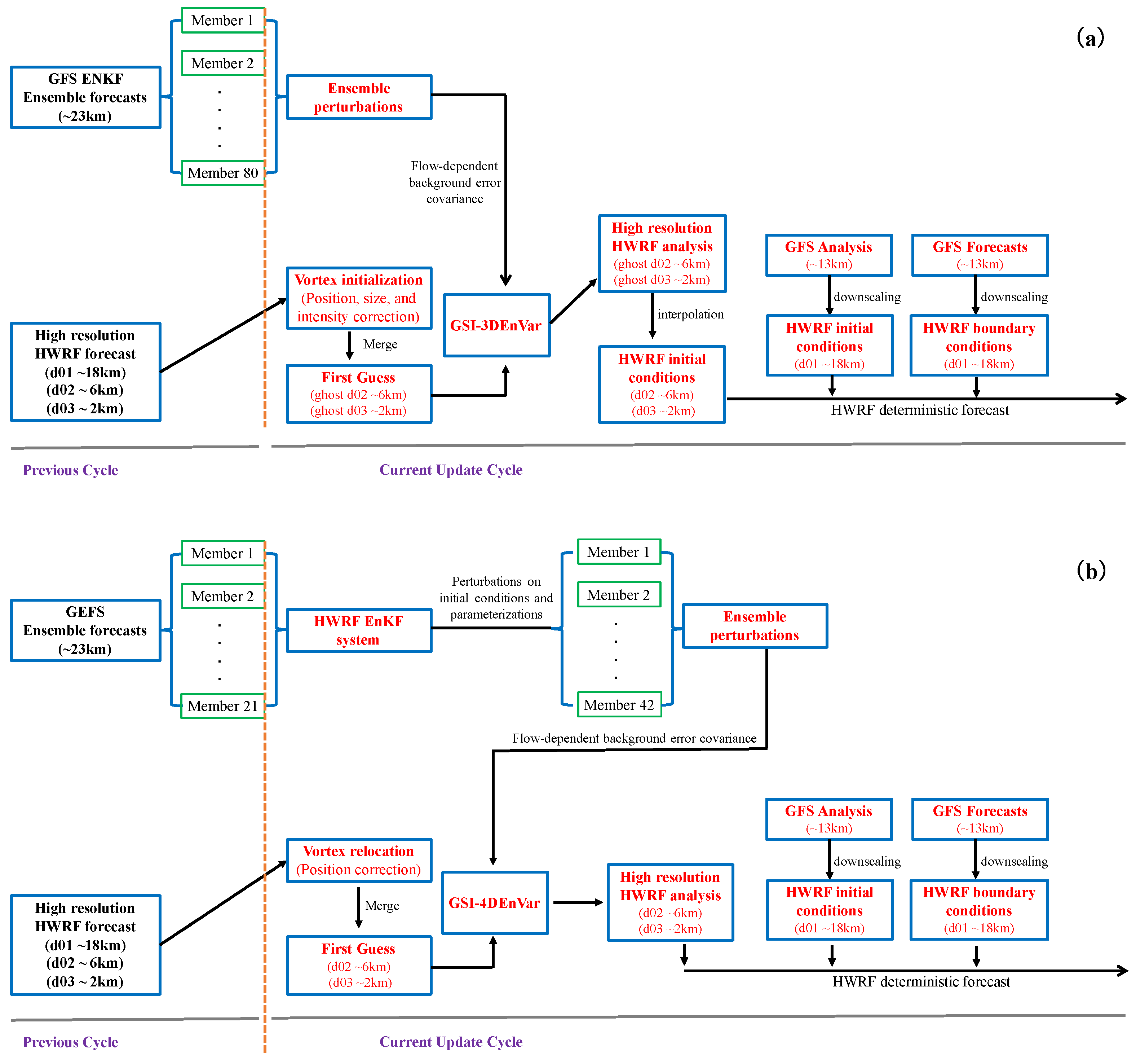
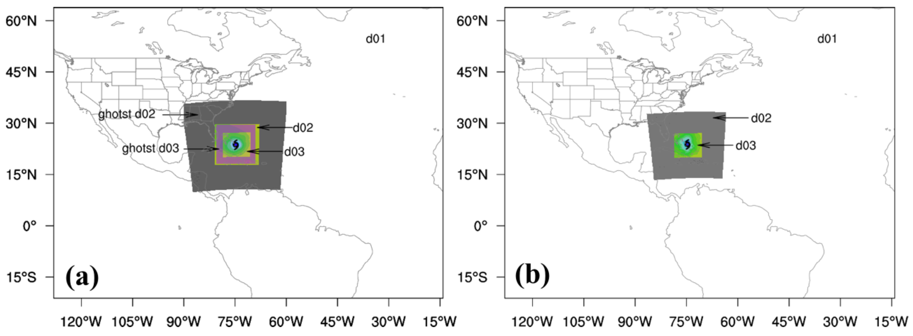
• VI is applied to the previous cycle’s HWRF forecasts in the d01 (∼18 km), d02 (∼6 km), and d03 (∼2 km) domains (see Figure 2a) to provide the first guess for DA. The VI enables the relocation, resizing, and intensity correction of the vortex using the NHC tropical cyclone vital statistics (TCVitals) database in order to correct the storm position and intensity approach to the real-time estimation.
• After VI, the improved initial conditions in d01, d02, and d03 are merged into two large domains, ghost d02 (∼6 km) and ghost d03 (∼2 km) (see Figure 2a). The ghost d02 and ghost d03 domains are an extension of forecast domains d02 and d03, respectively. The size of ghost d02 (ghost d03) is about two times larger than that of d02 (d03). The goal of this approach is to include more observations in the GSI-3DEnVar DA system for HWRF and to obtain a more realistic analysis near the domain boundaries of d02 and d03.
• Observations available for the operational HWRF are then assimilated into ghost d02 and ghost d03 by the GSI-3DEnVar system to further improve the initial conditions for the HWRF forecast. The 6-h NCEP operational GFS 80-member ensemble forecast at a resolution of T574 (∼23 km) from the previous analysis cycle is used to provide the flow-dependent background error covariance for GSI-3DEnVar within a 6-h DA window. We note that GSI-3DEnVar does not consider the temporal evolution of error covariances.
• After DA, the model fields in ghost d02 and ghost d03 are then interpolated back into the d02 and d03 domains to form the initial conditions of these two domains. The initial conditions in d01 are downscaled from GFS real-time analysis in the current HWRF analysis cycle. In addition, a “blending” scheme is activated after the VI and DA processes. This scheme blends the vortex from the VI process with the vortex after DA, and uses the blended vortex in the final analysis for the HWRF forecast. The effect of this scheme will eliminate the DA increments within 150 km of the center below 400 hPa. The details for this procedure can be referred to [10]. Moreover, the GFS forecasts are used to provide the boundary conditions for the HWRF model. With all of above information, the deterministic HWRF forecast during a specific period (e.g., 126 h) is made.

In this study, we evaluate the 4DEnVar initialization framework for HWRF. The differences between the 4DEnVar and 3DEnVar initialization frameworks are listed in

Table 1. Differences between the three-dimensional ensemble-variational (3DEnVar) and the four-dimensional ensemble-variational (4DEnVar) initialization frameworks for Hurricane Weather Research and Forecasting (HWRF).

Configuration	HWRF 3DEnVar Initialization Framework	HWRF 4DEnVar Initialization Framework
DA scheme	GSI-3D-EnVar	GSI-4D-EnVar
Flow-dependent error covariance	GFS 80-member ensembles (∼23 km)	HWRF 42-member ensembles (∼6 km)
Vortex initialization	Vortex relocation & Intensity correction	Vortex relocation
DA domains	ghost d02 (30${}^{°}$ × 30${}^{°}$)	d02 (25${}^{°}$ × 25${}^{°}$)
	ghost d03 (12${}^{°}$ × 12${}^{°}$)	d03 (7.5${}^{°}$ × 9${}^{°}$)
Forecast domains	d01 (80${}^{°}$ × 80${}^{°}$)	d01 (80${}^{°}$ × 80${}^{°}$)
	d02 (13${}^{°}$ × 13${}^{°}$)	d02 (25${}^{°}$ × 25${}^{°}$)
	d03 (7.5${}^{°}$ × 9${}^{°}$)	d03 (7.5${}^{°}$ × 9${}^{°}$)

. In addition, as shown in Figure 1b, the HWRF simulation with this initialization framework contains the following steps:

• A parallel run of the HWRF regional ensemble system [26] initialized by the forecasts from the Global Ensemble Forecast System (GEFS) is performed first to generate a 42-member self-consistent HWRF ensemble at 6-km resolution. Here, the self-consistent means that the ensemble forecasts use the same resolution and model configurations as the HWRF model. The detailed treatments and parameters used for HWRF ensemble forecasts follow those in Zhang et al. [26]. These 42-member self-consistent HWRF ensembles (6 km) are then used to provide the flow-dependent background error covariances for the GSI-4DEnVar DA system in 4DEnVar initialization framework. In this way, the DA system considers the temporal evolution of error covariances via the use of four-dimensional ensemble perturbations that are provided by high-resolution, self-consistent HWRF ensemble forecasts.
• Vortex relocation is performed on the previous cycle’s HWRF forecasts in the d02 (∼6 km) and d03 (∼2 km) domains (see Figure 2b) before DA. Vortex relocation corrects the storm position based on the NHC tropical cyclone vital statistics (TCVitals) database without changes in storm size and intensity. In addition, the size of d02 in Figure 2b for 4DEnVar initialization framework is about two times larger than that in Figure 2a for the 3DEnVar initialization framework, which is used to include more observations in the GSI-4DEnVar system and to obtain a more realistic analysis in the storm environment. The sizes of d01 and d03 in Figure 2b are the same as those in Figure 2a.
• After vortex relocation, the observations available for operational HWRF are then assimilated directly into d02 and d03 by the GSI-4DEnVar system to further improve the initial conditions in these domains. In GSI-4DEnVar, the DA window is divided into 6 observational bins; the 3-h, 4-h, 5-h, 6-h, 7-h, 8-h, and 9-h self-consistent HWRF 42-member ensemble forecasts from the first step are used to provide the flow-dependent background error covariance, realizing the time evolution of background error covariance within a 6-h DA window. We note that the 1-h observational bins are used in this study for GSI-4DEnVar as the previous study has demonstrated that the performance of GSI-4DEnVar can be enhanced with a denser observational bin [19].
• As in the 3DEnVar initialization framework, the initial conditions in d01 (Figure 2b) for 4DEnVar initialization framework are also downscaled from the GFS real-time analysis in the current HWRF analysis cycle. This is combined with the analyses from the above step for d02 and d03 to provide the initial conditions for the HWRF forecast. The GFS forecasts are still used to provide the boundary conditions. Finally, a deterministic HWRF forecast for a specific time period (e.g., 126 h) can be made.

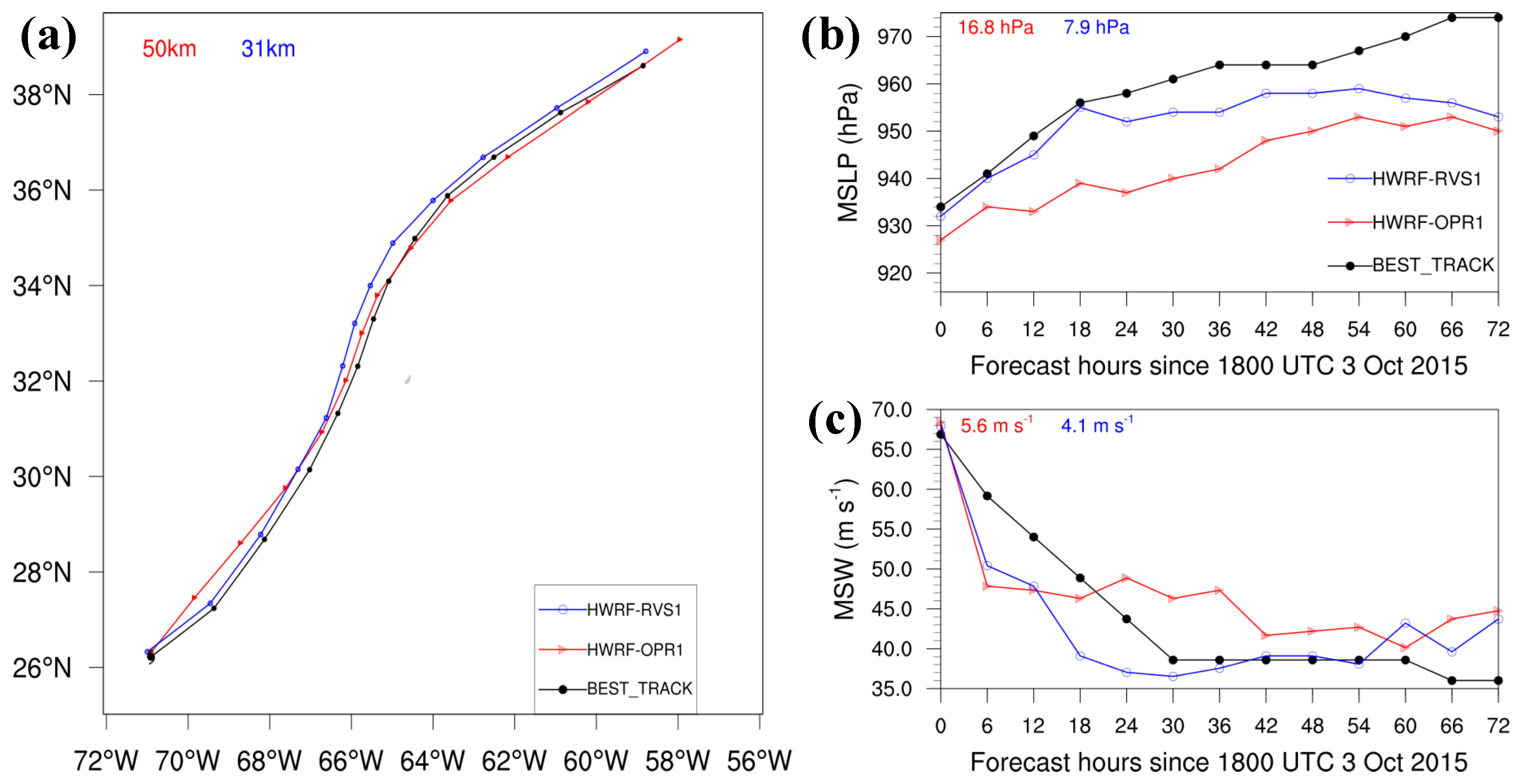
3. Performances on the Simulation of the Rapid Weakening of Hurricane Joaquin

In this section, the performances of HWRF analyses and forecasts with two different initialization frameworks are compared. Hurricane Joaquin, which occurred over the Atlantic Ocean in the 2015 hurricane season, is selected as a case study. A detailed description of this case can be seen in Berg [27]. Since this study focuses on forecasts of TC intensity changes, the initialization and HWRF simulation are performed on the rapid weakening (RW) phase of Hurricane Joaquin from 1800 UTC 02 to 1800 UTC 06 October 2015. The HWRF model is initialized at 1200 UTC 02 October 2015 and allowed to spin-up until 1800 UTC 02 October 2015, and then a DA process is performed and cycled from 1800 UTC 02 to 1800 UTC 03 October 2015 in 6-h windows, for a total of 24-h. All datasets available for the operational HWRF (see the list of types at [22]), along with available high-resolution Tail Doppler Radar (TDR) and HDSS dropsonde observations, are assimilated. After DA, a 72-h forecast from 1800 UTC 03 to 1800 UTC 06 October 2015 is then performed to predict the RW of Hurricane Joaquin. We note that the 72-h forecast period is selected as it has already covered the whole intensity changes period for Hurricane Joaquin, thus, we did not run a 5-day simulation following the HWRF routines to save the computational time. Two experiments are conducted: HWRF-OPR1 and HWRF-RVS1. HWRF-OPR1 adopts the 3DEnVar initialization framework (Figure 1a), while HWRF-RVS1 uses the 4DEnVar initialization framework (Figure 1b).

Table 2. List of experiments.

Exps.	HWRF Initialization	Hurricane Case	DA Period a	Simulation Period
HWRF-OPR1	3DEnVar (Figure 1a)	Joaquin (2015)	1800 UTC 02–1800 UTC 03 October	1800 UTC 03–1800 UTC 06 October
HWRF-RVS1	4DEnVar (Figure 1b)	Joaquin (2015)	1800 UTC 02–1800 UTC 03 October	1800 UTC 03–1800 UTC 06 October
HWRF-OPR2	3DEnVar (Figure 1a)	Patricia (2015)	1800 UTC 20–1800 UTC 21 October	1800 UTC 21–1800 UTC 24 October
HWRF-RVS2	4DEnVar (Figure 1b)	Patricia (2015)	1800 UTC 20–1800 UTC 21 October	1800 UTC 21–1800 UTC 24 October
HWRF-OPR3	3DEnVar (Figure 1a)	Matthew (2016)	1800 UTC 28–1800 UTC 29 September	1800 UTC 29 September–1800 UTC 02 October
HWRF-RVS3	4DEnVar (Figure 1b)	Matthew (2016)	1800 UTC 28–1800 UTC 29 September	1800 UTC 29 September–1800 UTC 02 October

^a The observations that are assimilated by each simulation include conventional and satellite observations, as well as HDSS dropsonde and Tail Doppler Radar (TDR) radial wind data.

summarizes all experiments and their acronyms.

3.1. Balances in HWRF Initial Conditions

A previous study has proved that gradient imbalances exist in the initial conditions with the operational HWRF initialization framework in some cases due to the use of VI before DA, leading to the vortex spin-down problems and the degradation of the intensity forecast [9]. Thus, we first investigate whether the 4DEnVar initialization framework can alleviate this problem. Following Pu et al. [9], the azimuthally averaged net radial force F, which represents the difference between the local radial pressure gradient and the sum of the centrifugal and Coriolis forces, is calculated to examine the dynamical balances in the HWRF initial vortices generated by the two different initialization frameworks.

Figure 3a,b shows the radius–height cross-sections of F isopleths before and after VI in HWRF-OPR1 at 1800 UTC 03 October 2015 (analysis time). It clearly reveals the strong supergradient wind fields in the inner-core region of the vortex after the VI procedure (Figure 3b), indicating that VI induces these supergradient wind fields. DA in HWRF-OPR1 does not eliminate the supergradient wind fields, as the distribution and magnitude of F in Figure 3c are nearly the same as in Figure 3b. However, the distribution and magnitude of F in HWRF-OPR1 are adjusted significantly after the 3-h forecast (Figure 3d). As a result, the gradient wind balance is established in the inner core region with a radius < 50 km, and the supergradient and subgradient wind fields are concentrated around the radius of maximum wind (Figure 3d). This indicates that the supergradient wind fields induced by VI in Figure 3b,c are not realistic, and the model has to adjust these imbalanced structures in the first few hours’ forecasts.

In contrast to HWRF-OPR1, the gradient wind fields are much more balanced in HWRF-RVS1 before (Figure 3e) and after VI (Figure 3f). We note that the VI in HWRF-OPR1 enables both the vortex relocation and intensity correction, while VI in HWRF-REV1 only enables only the vortex relocation, as shown in Table 1. Thus, the results in Figure 3f suggest that the intensity correction in VI for HWRF-OPR1 is responsible for the strong supergradient wind fields (or gradient wind imbalances) in the inner-core region in Figure 3b. In addition, DA in HWRF-RVS1 does not largely affect the gradient wind balances (Figure 3g), and no significant adjustment is revealed during the first 3-h forecast period (Figure 3h). Overall, the 4DEnVar initialization framework can improve the balances in the initial conditions for HWRF by removing the empirical intensity correction in VI.

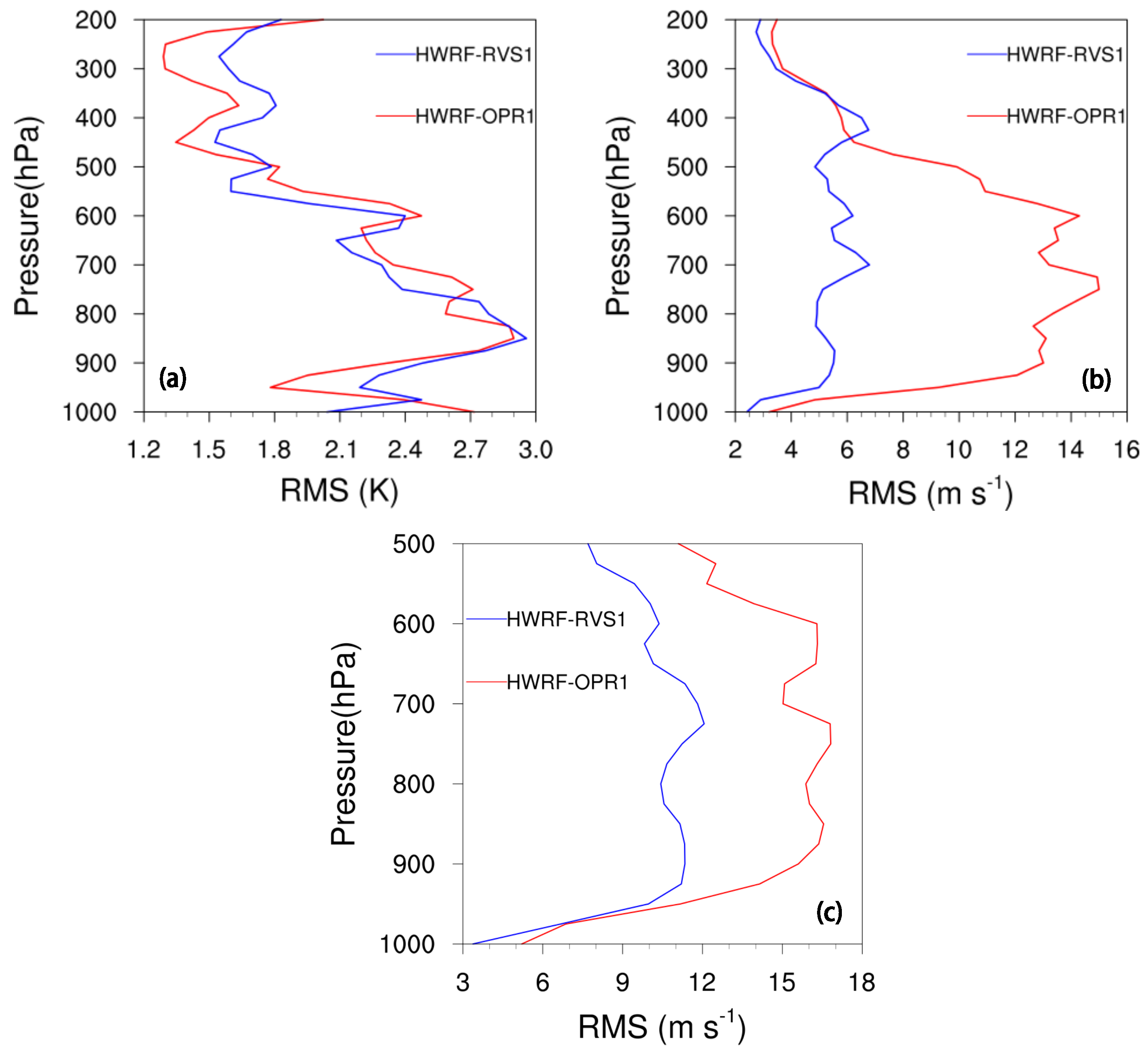
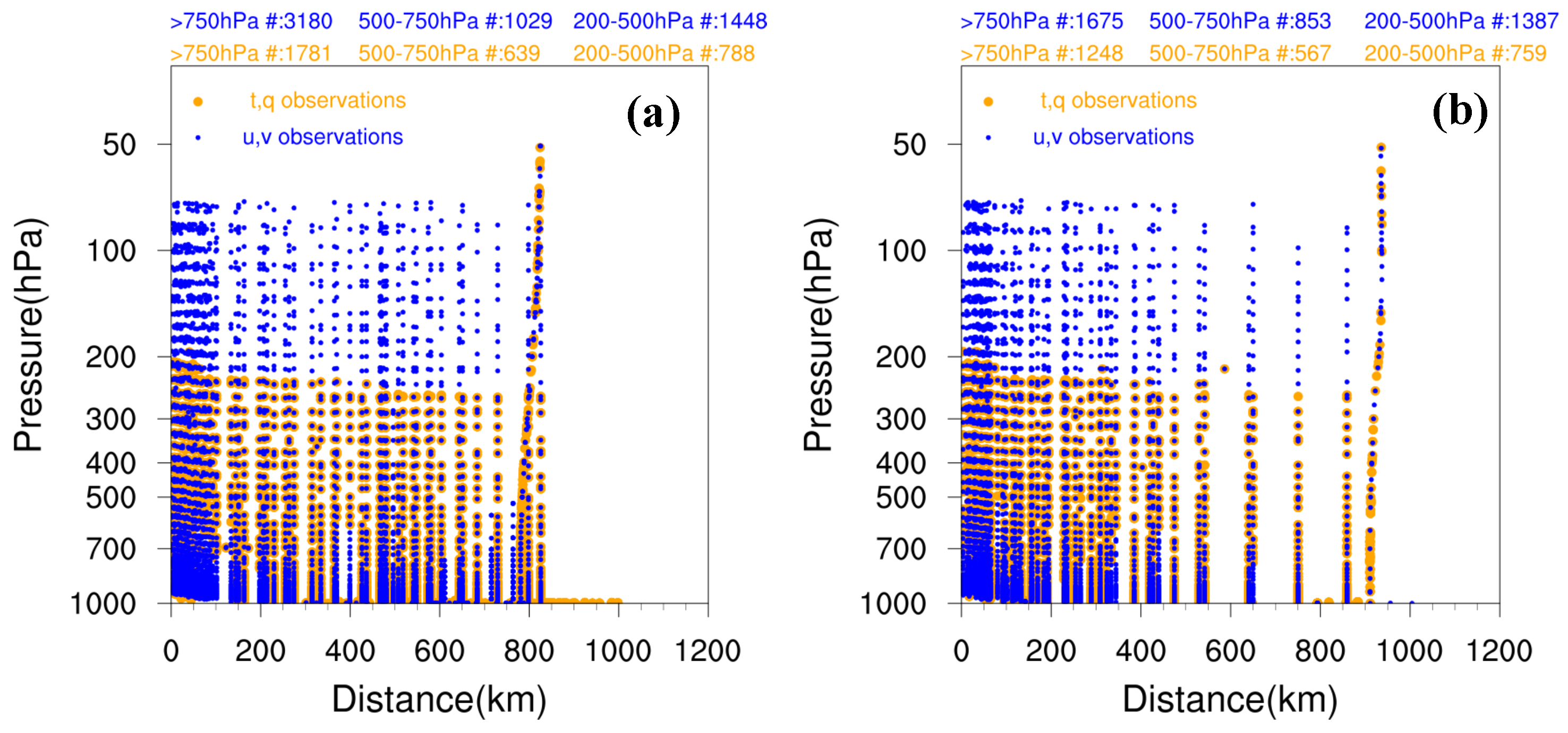
3.1.1. Fit to Observations

The 4DEnVar initialization framework can enhance the performance of DA. Figure 4a,b shows the root-mean-square (RMS) fit of the analysis to in-situ observations within the d02 region (Table 1), averaged over the DA period from 1800 UTC 02 to 1800 UTC 03 October 2015. The analyzed temperature from HWRF-RVS1 and HWRF-OPR1 fit the observational temperature similarly, except that HWRF-RVS1 leads to a slightly better fit in the midlevel (750–500 hPa) than HWRF-OPR1 does (Figure 4a). In addition, the root-mean-square fit of the analyzed wind to observations is significantly improved by HWRF-RVS1. As shown in Figure 4b, the RMS of wind speed within 900–500 hPa in HWRF-RVS1 is about 2–3 times smaller than that in HWRF-OPR1. Overall, the analyses from HWRF-RVS1 lead to a better fit of the analysis to the observations than HWRF-OPR1 does, but the improvements are mainly seen in the dynamical fields (u, v wind) rather than thermal fields (i.e., temperature and humidity). One possible reason for the improvements in HWRF-RVS1 (Figure 4a) is that the size of domain d02 in HWRF-RVS1 is about two times larger than the d02 domain in HWRF-OPR1 (see Table 1), which allows more information from data assimilation to be kept in the initial conditions that are used for the HWRF forecast. In HWRF-OR1, only the information within the two forecast domains with smaller domain sizes (i.e., d02 and d03) are used for the HWRF forecast, although the data assimilation is performed on the two large domains (i.e., ghost d02 and d03).

Figure 5 further shows the distribution of observations that are assimilated by GSI at 1800 UTC 02 and 1800 UTC 03 October 2015. We can see that two times more wind observations are assimilated by the HWRF DA system relative to the temperature and humidity data (see the numbers at the top of Figure 5a,b). This partially explains why the results from HWRF-RVS1 show significant improvement in the wind but much less significant improvement in temperature in Figure 4. In addition, Figure 5 reveals that the temperature and humidity observations within the inner-core region are mostly concentrated in the boundary layer regions (below 700 hPa), while the observations are much sparse in the middle (500–750 hPa) and upper levels (200–500 hPa). In particular, there are no temperature and humidity observations within the inner-core region (radius < 800 km) above 200 hPa (Figure 5). In this way, we would expect the worse root-mean-square fit of the analyzed temperature to observations in the upper levels (above 500 hPa), as shown in Figure 4a.

Figure 4c further illustrates the root-mean-square (RMS) fit of the analyzed wind speed to in-situ observations within the d03 region (Table 1), averaged over the DA period from 1800 UTC 02 to 1800 UTC 03 October 2015. We can see that HWRF-RVS1 produces a much smaller RMS of wind speeds extended from 900 hPa to 500 hPa than HWRF-OPR1 does. Two factors in the 4DEnVar initialization framework can contribute to the improvements in the HWRF analysis in HWRF-RVS1: first, the use of high-resolution flow-dependent error covariances in HWRF-RVS1. Figure 6a,b show the ensemble spreads of temperature at 850 hPa from the 80-member GFS EnKF ensembles for HWRF-OPR1 and the 42-member HWRF regional ensembles for HWRF-RVS1 at 1800 UTC 03 October 2015. Apparently, the 42-member HWRF ensemble members provide many detailed storm-scale structural features for temperature (Figure 6b) compared with the 80-member global ensembles (Figure 6a). The same features are also observed in the wind and relative humidity fields (Figures not shown). Compared with the coarser-resolution global ensemble forecasts, high-resolution regional ensemble forecasts in the HWRF native model domains can produce much more realistic (storm-scale) correlation structures among these variables and enable DA to incorporate the convective-scale information from observations into the HWRF analysis. Second, the flow-dependent background error covariances in HWRF-RVS1 evolve with time within a 6-h DA window. As shown in Figure 6c–h, the ensemble spreads of temperature in HWRF-RVS1 reveal different structures at different times within the DA window. The variation of the ensemble perturbations within the DA window will give the DA system a greater ability to capture the high-frequency changes in atmospheric variables in the observational field (e.g., wind field). With these advantages, 4DEnVar initialization framework can better incorporate the observational information related to TCs into the HWRF initial conditions, relative to the operational initialization framework. As a result, the analysis field in HWRF-RVS1 is more realistic than that in HWRF-OPR1, and the RMS errors of wind in HWRF-RVS1 are smaller than those in HWRF-OPR1.

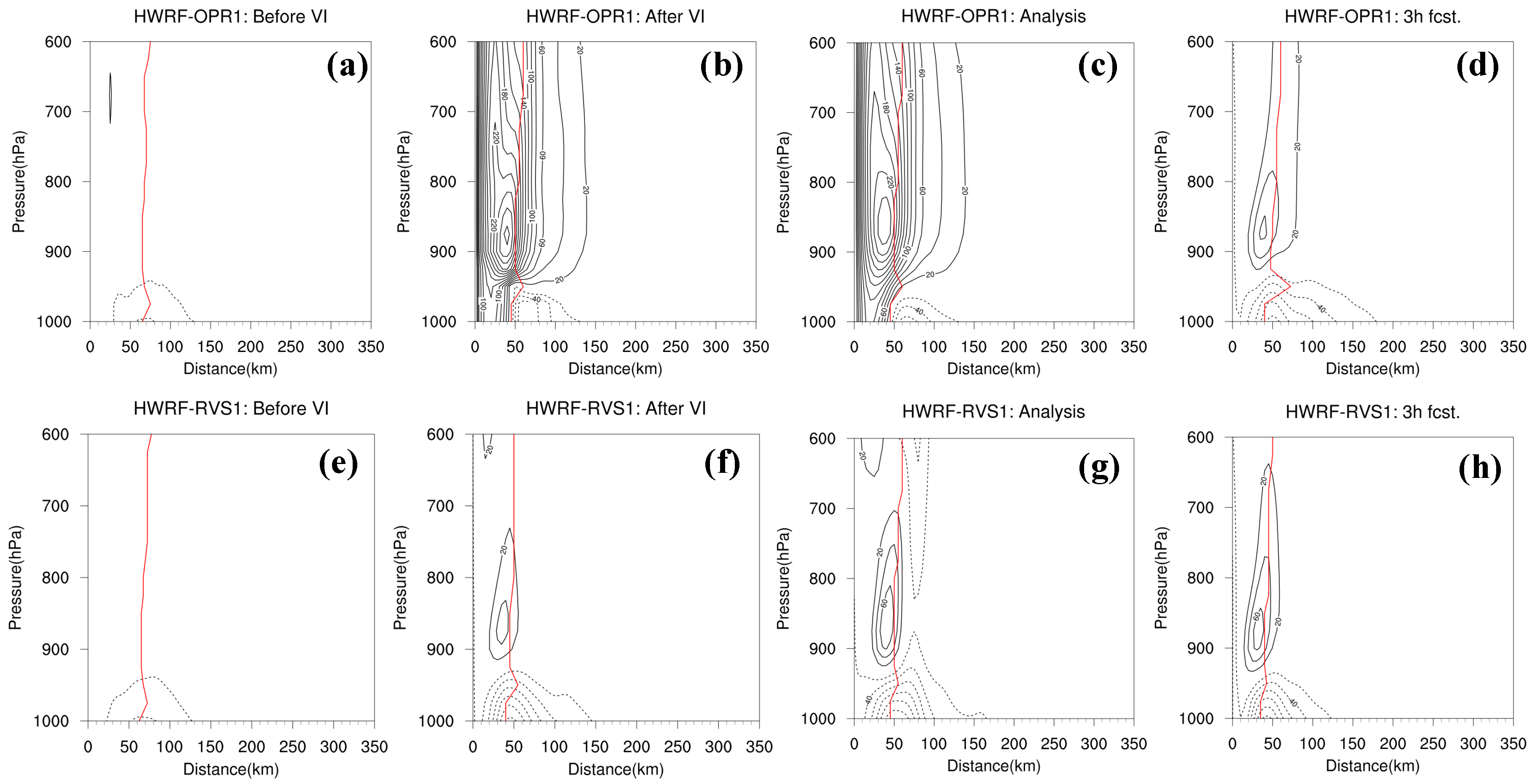
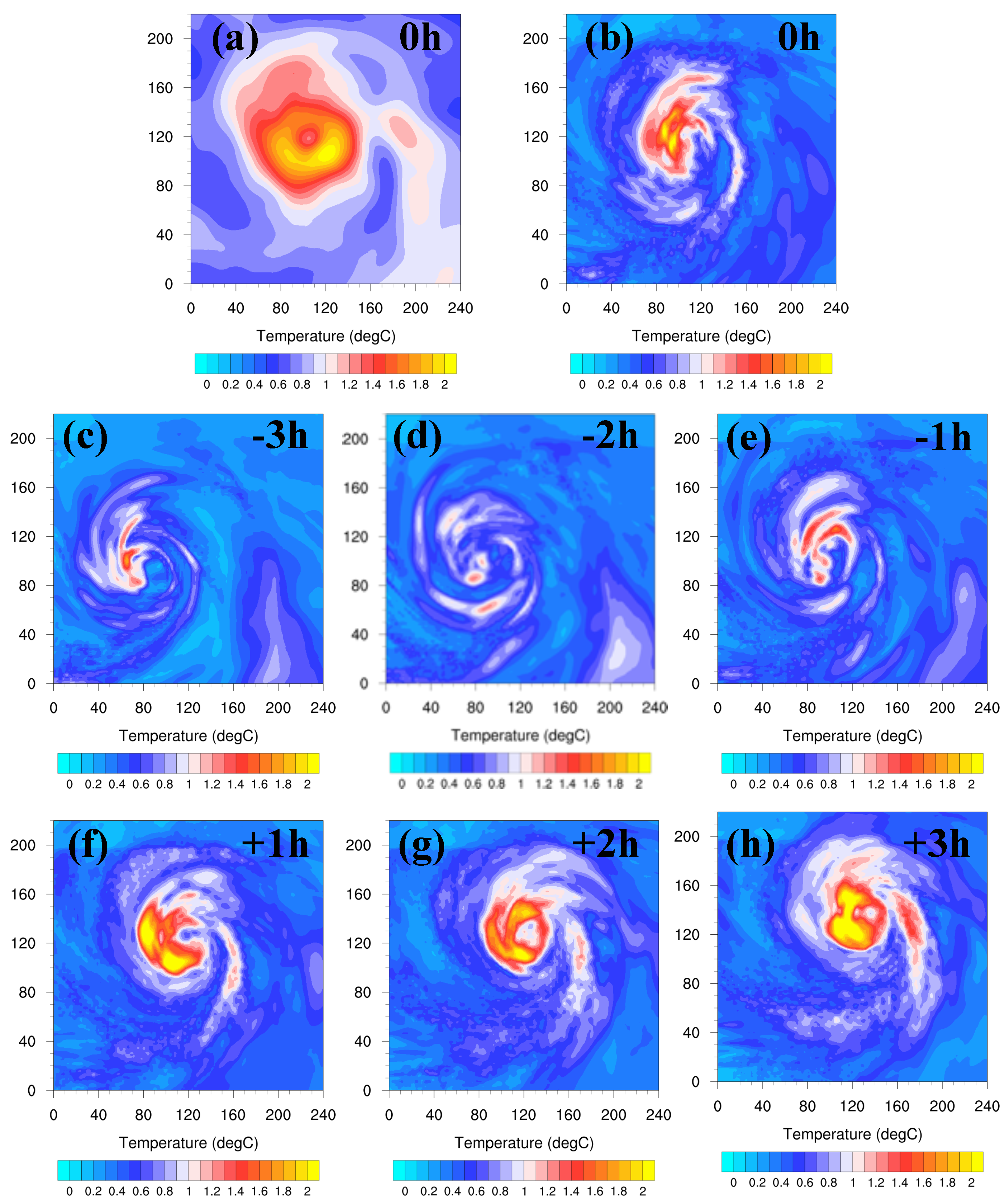
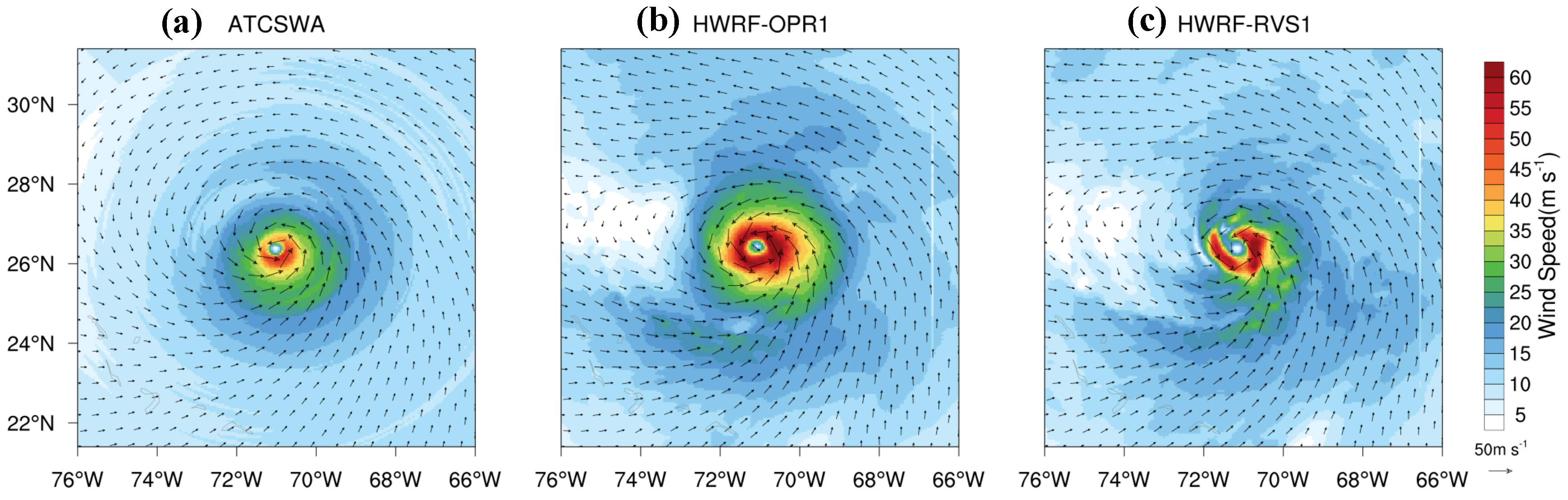
3.1.2. Analysis of Storm Structure

The improvement of the fit of analyzed wind speed to the in-situ observations in HWRF-RVS1 implies that HWRF-RVS1 may produce better analyzed wind structure than HWRF-OPR1 does. Figure 7 illustrates the 10-m wind analysis field from HWRF-OPR1 and HWRF-RVS1, compared against the Aircraft-based Tropical Cyclone Surface Wind Analysis (ATCSWA) provided by the National Oceanic and Atmospheric Administration/National Environmental Satellite Data and Information Service (NOAA/NESDIS). Previous studies [28,29] have proven that the basic vortex structure can be well reproduced by ATCSWA data. Thus, the ATCSWA can be used to evaluate the vortex structure in the HWRF analysis and forecast. Compared with the ATCSWA wind field across the center of Hurricane Joaquin (Figure 7a), the HWRF-OPR1 analysis at 1800 UTC 03 October 2015 (Figure 7b) overestimates the maximum wind speed in the inner-core region and fails to capture the asymmetric vortex structure, as shown in ATCSWA. In contrast, the HWRF-RVS1 analysis (Figure 7c) reproduces a more reasonable magnitude of maximum wind speed than HWRF-OPR1 does and captures the asymmetric wind structure, as shown in ATCSWA. Thus, 4DEnVar initialization framework produces a more realistic surface wind structure than the operational initialization framework does.

3.1.3. HWRF Forecast

The two initialization frameworks also lead to different HWRF forecasts during the rapid weakening of Hurricane Joaquin. Figure 8 illustrates the RMS errors for temperature, specific humidity, and wind forecasts with the HWRF-OPR1 and HWRF-RVS1 experiments verified against the HDSS dropsonde observations at 1800 UTC 04 and 1800 UTC 05 October 2015 over the innermost domain (d03, Table 1). The HDSS dropsonde observations are from the Tropical Cyclone Intensity (TCI) 2015 field campaign [30]. The data is quality controlled using a combined “subjective-objective” procedure which utilizes the Atmospheric Sounding Processing Environment (ASPEN) software (Bell et al. 2016). After the quality control, there are 74 (80) total profile observations at 1800 UTC 04 (05) October 2015. In this study, the grid point values of temperature, specific humidity and wind speed from HWRF simulations are first interpolated into a HDSS dropsonde observational point, then the average RMS errors between the HWRF forecasts and HDSS dropsondes are calculated and compared. As shown in Figure 8, the RMS errors of temperature, specific humidity, and wind speed at the 24-h and 48-h forecasts in HWRF-RVS1 (blue lines) are smaller than those in HWRF-OPR1 (red lines). This indicates that the forecasts produced by HWRF-RVS1 are more skillful than those of HWRF-OPR1. In addition, the reduction in the RMS errors of wind in HWRF-RVS1 is significant in both the 24-h and 48-h forecasts, whereas the reduction in the RMS errors of temperature and specific humidity are significant only in the 24-h forecast.

Figure 9 further shows the track and intensity in terms of the minimum sea level pressure (MSLP) and maximum surface wind (MSW) produced by the two different initialization frameworks from 1800 UTC 03 October to 1800 UTC 06 October 2015. It is verified that HWRF-RVS1 leads to better track and intensity forecasts than HWRF-OPR1 does. Specifically, both HWRF-OPR1 and HWRF-RVS1 produce realistic track forecasts, as the track errors over a 72-h forecast period are less than 60 km (Figure 9a). However, the cross-track errors in the first 12-h and the along-track errors after the 48-h forecast in HWRF-OPR1 are reduced in HWRF-RVS1. As a result, HWRF-RVS1 leads to a 37% average track error reduction over the 72-h forecast period compared with HWRF-OPR1 (Figure 9a). As for the intensity forecasts, HWRF-RVS1 reduces the 72-h averaged MSLP and MSW errors in HWRF-OPR1 by 53% and 26%, respectively (Figure 9b,c). More importantly, the unrealistic wind-pressure relationship in HWRF-OPR1 is eliminated by HWRF-RVS1, as the overestimation of MSLP in HWRF-OPR1 is significantly mitigated by HWRF-RVS1.

Quantitative wind and precipitation forecasts from the two different initialization frameworks are also diagnosed. Figure 10 shows the distribution of the 10-m wind field from the 24-h forecast of HWRF-OPR1 and HWRF-RVS1, compared against the 10-m wind analysis from ATCSWA at 1800 UTC 03 October 2015. Relative to ATCSWA (Figure 10a), the large overestimation of wind speed around the storm center in HWRF-OPR1 (Figure 10b) is not seen in HWRF-RVS1 (Figure 10c). In addition, HWRF-RVS1 (Figure 10c) partially captures the asymmetric wind structure shown in ATCSWA (Figure 10a), whereas HWRF-OPR1 (Figure 10b) leads to symmetric wind structure. Therefore, HWRF-RVS1 leads to a more realistic storm structure forecast than HWRF-OPR1 does. Following Wang (2014), mean equitable threat scores (ETSs) are further calculated for the forecasted 10-m wind fields from HWRF-OPR1 and HWRF-RVS1 compared against the ATCSWA wind analysis fields during the rapid weakening of Hurricane Joaquin from 1800 UCT 03 to 0000 UTC 05 October 2015. The ETS measures the quantitatively forecast accuracy relative to the observational or analysis field. As depicted in Figure 10d, the mean ETSs in HWRF-RVS1 are higher than those in HWRF-OPR1 for all the thresholds from 10 $\mathrm{m}{\mathrm{s}}^{-1}$ to 50 $\mathrm{m}{\mathrm{s}}^{-1}$, indicating that HWRF-RVS1 produces more skillful wind forecasts during the whole rapid weakening of Hurricane Joaquin than HWRF-OPR1 does.

Figure 11 also illustrates the 30-h accumulated precipitation distribution during the rapid weakening of Hurricane Joaquin from 1800 UTC 03 to 0000 UTC 05 October 2015, compared with precipitation observations from the Tropical Rainfall Measuring Mission (TRMM) 3B42 products. It is clear that HWRF-OPR1 (Figure 11b) produces too much rainfall along the storm track relative to TRMM 3B42 (Figure 11a), while HWRF-RVS1 captures the magnitude and distribution of precipitation below 30${}^{°}$ N in TRMM 3B42 (Figure 11a,c), and the overall precipitation distribution in HWRF-RVS1 (Figure 11c) is much more realistic than that in HWRF-OPR1 (Figure 11b). In order to quantitatively verify the precipitation forecasts (QPFs) in HWRF-OPR1 and HWRF-RVS1, ETSs are also calculated for the 30-h accumulated precipitation from HWRF-OPR1 and HWRF-RVS1 compared with the precipitation observations from TRMM 3B42. As shown in Figure 11d, the ETSs in HWRF-RVS1 are higher than those in HWRF-OPR1 for all thresholds from 10 mm to 150 mm, indicating that HWRF-RVS1 also produces more skillful precipitation forecasts during the rapid weakening of Hurricane Joaquin than HWRF-OPR1 does.

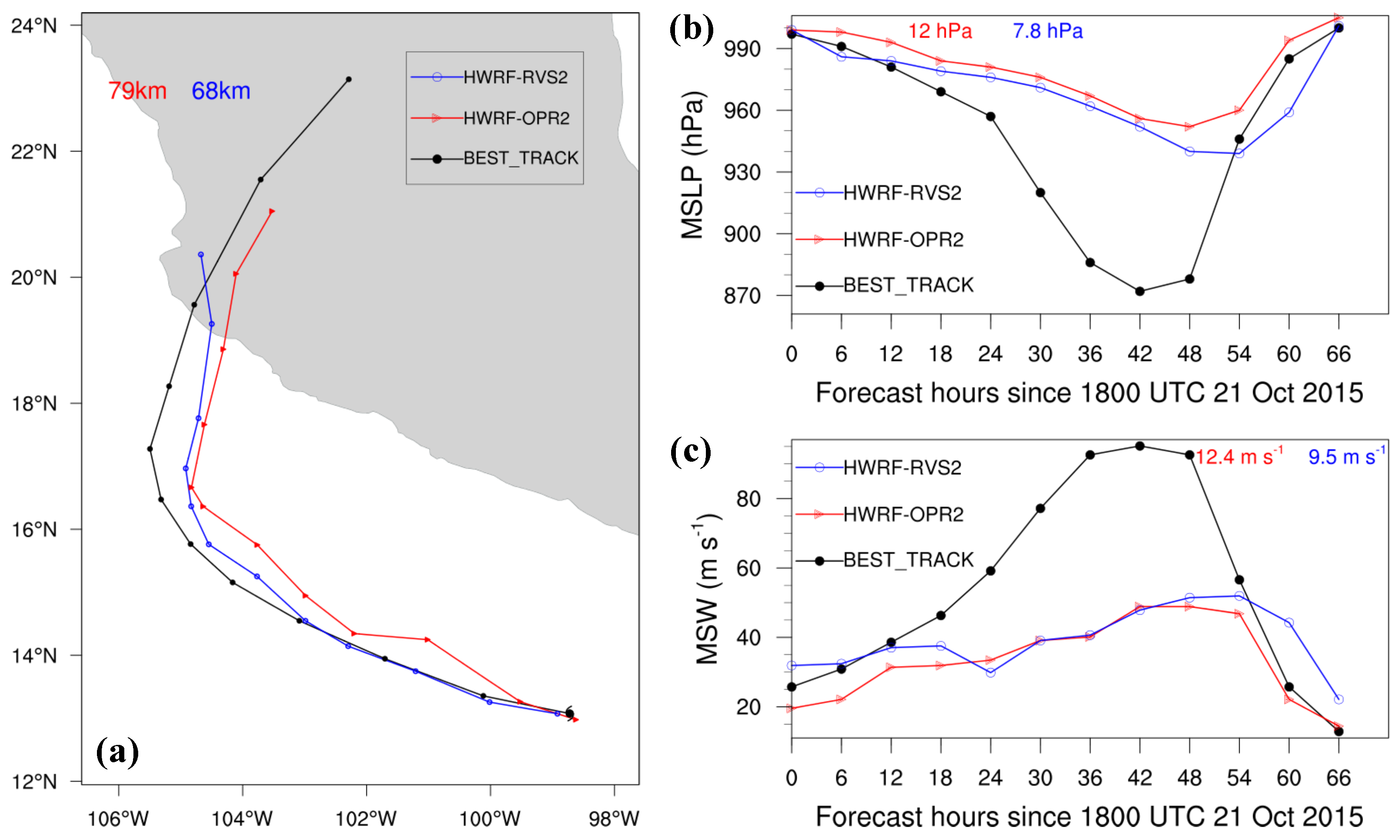
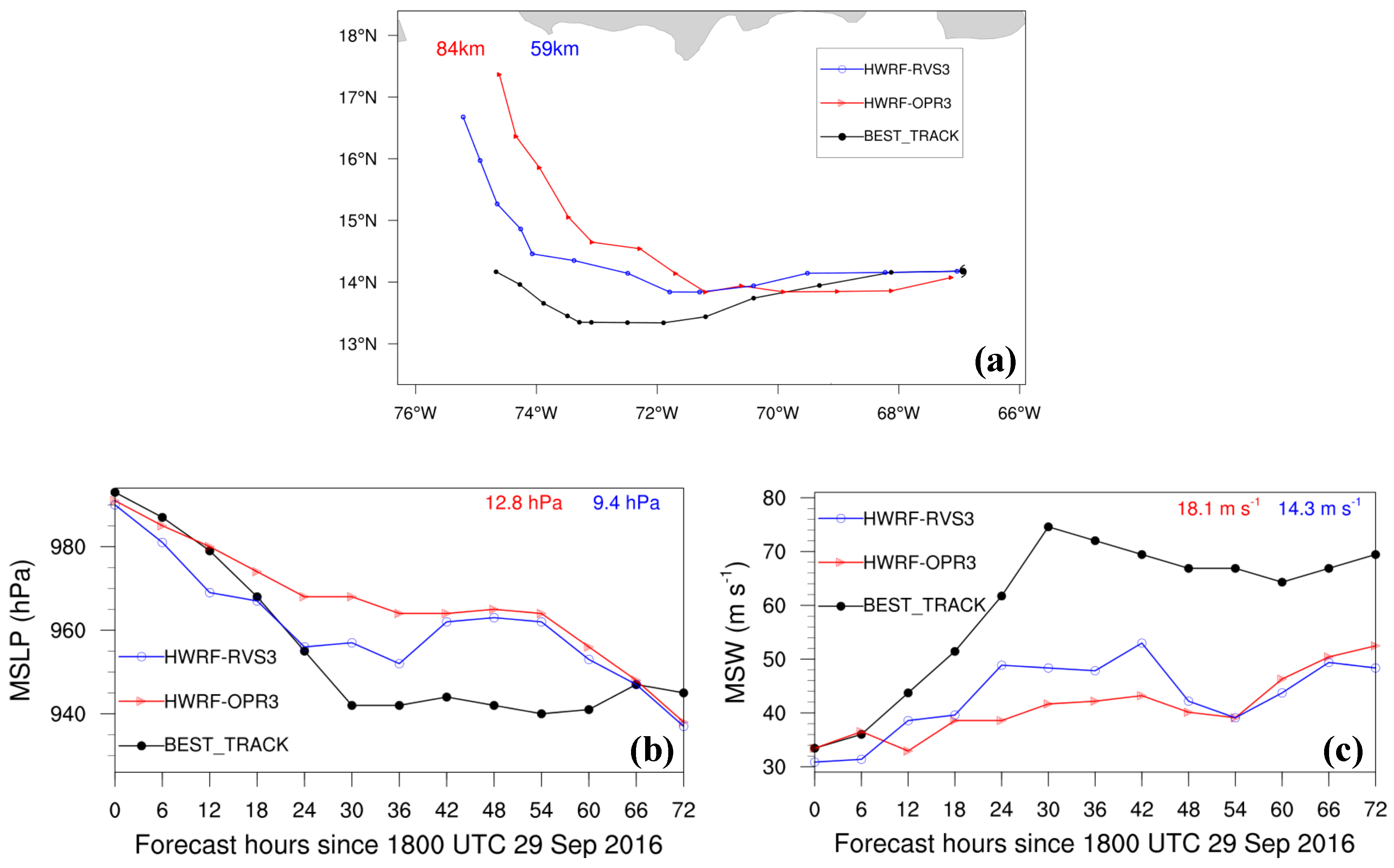
4. Forecasts of the Rapid Intensification of Hurricanes Patricia and Matthew

As we have shown in the previous section, the 4DEnVar initialization framework leads to a more skillful forecast of TC intensity change than the 3DEnVar initialization framework does. In order to further confirm these results, HWRF simulations with two different HWRF initialization frameworks are also conducted on Hurricanes Patricia and Matthew during their rapid intensification period. Detailed descriptions of these two cases can be found in Kimberlain et al. [31] and Stewart [32], respectively. For Hurricane Patricia, the HWRF model is initialized at 1200 UTC 20 October 2015, the model is allowed to spin-up until 1800 UTC 20 October 2015, and then a DA process is performed that is cycled from 1800 UTC 20 to 1800 UTC 21 October 2015 every 6-h, for a total of 24-h. A 66-h forecast from 1800 UTC 21 to 1200 UTC 24 October 2015 is then performed to predict intensity changes of Hurricane Patricia. For Hurricane Matthew, the HWRF model is initialized at 1200 UTC 28 September 2016, allowed to spin-up until 1800 UTC 28 September 2016, and the cycled DA is performed from 1800 UTC 28 to 1800 UTC 29 September 2016 in 6-h windows, for a total of 24-h. Finally, a 72-h forecast from 1800 UTC 29 to 1800 UTC 02 October 2016 is made to simulate the period of intensity changes of Hurricane Matthew. As with Hurricane Joaquin, two HWRF experiments are designed for Hurricanes Patricia (Matthew) to understand the effects of the two different initialization frameworks. Details of the experimental design are listed in Table 2.

Figure 12 shows the track and intensity in terms of minimum sea level pressure (MSLP) and maximum surface wind (MSW) produced by the two different initialization frameworks for Hurricane Patricia from 1800 UTC 21 to 1200 UTC 24 October 2015. Overall, the rapid intensification of Hurricane Patricia is not well captured by either HWRF-OPR2 or HWRF-RVS2 (Figure 12b,c). However, HWRF-RVS2 outperforms HWRF-OPR2 in track, MSLP, and MSW forecasts (Figure 12a–c). Compared with HWRF-OPR2, the mean track, MSLP, and MSW errors over the first 24-h forecast in HWRF-RVS2 are reduced by 14%, 35%, and 23%, respectively. In addition, HWRF-RVS2 leads to smaller cross-track errors than HWRF-OPR2 over the whole 66-h simulations.

Furthermore, Figure 13 illustrates the 72-h track and intensity forecasts for Hurricane Matthew during its rapid intensification from 1800 UTC 29 September to 1800 UTC 02 October 2016. It is clear that HWRF-RVS1 outperforms HWRF-OPR1 in terms of track, MSLP, and MSW forecasts (Figure 13a–c). Compared with HWRF-OPR1, the mean track, MSLP, and MSW errors over the first 48-h forecast in HWRF-RVS1 are reduced by 30%, 27%, and 21%, respectively. More importantly, the intensification of Hurricane Matthew in the first 24-h is well captured by HWRF-RVS1, as the track, MSLP, and MSW forecasts are nearly the same as those in the best-track data. Overall, the results for Hurricanes Patricia and Matthew further suggest that 4DEnVar initialization framework indeed improves forecasts of TC intensity change in HWRF.

5. Concluding Remarks

This study examined the forecast skill of TC intensity changes in a research version of the HWRF model with two different initialization frameworks. The first initialization framework is similar to that used in the operational HWRF, which employs the GSI-3DEnVar DA system with background error covariances provided by the coarser-resolution GFS EnKF ensembles. The second initialization framework is different from the first one, it uses GSI-4DEnVar with background error covariances provided by high-resolution self-consistent HWRF ensembles. Various HWRF simulations with the two different initialization frameworks are performed on three major hurricanes, including Joaquin, Patricia, and Matthew, during their intensity changes. The results suggest that:

• 4DEnVar initialization framework has shown the potential of leading to a better HWRF forecast of Hurricanes Joaquin, Patricia, and Matthew during their changes in intensity. Compared with the simulations with the 3DEnVar initialization framework, the 4DEnVar initialization framework leads to a reduction in track, MSLP, and MSW forecast errors, at least in the first 24-h forecast in all the HWRF simulations. However, the extent of the improvement is sensitive to the specific case. Specifically, the 4DEnVar initialization framework produces substantial improvements in the forecast of the rapid weakening of Hurricane Joaquin, while it produces weak improvements in the forecasts of the rapid intensification of Hurricanes Patricia and Matthew.
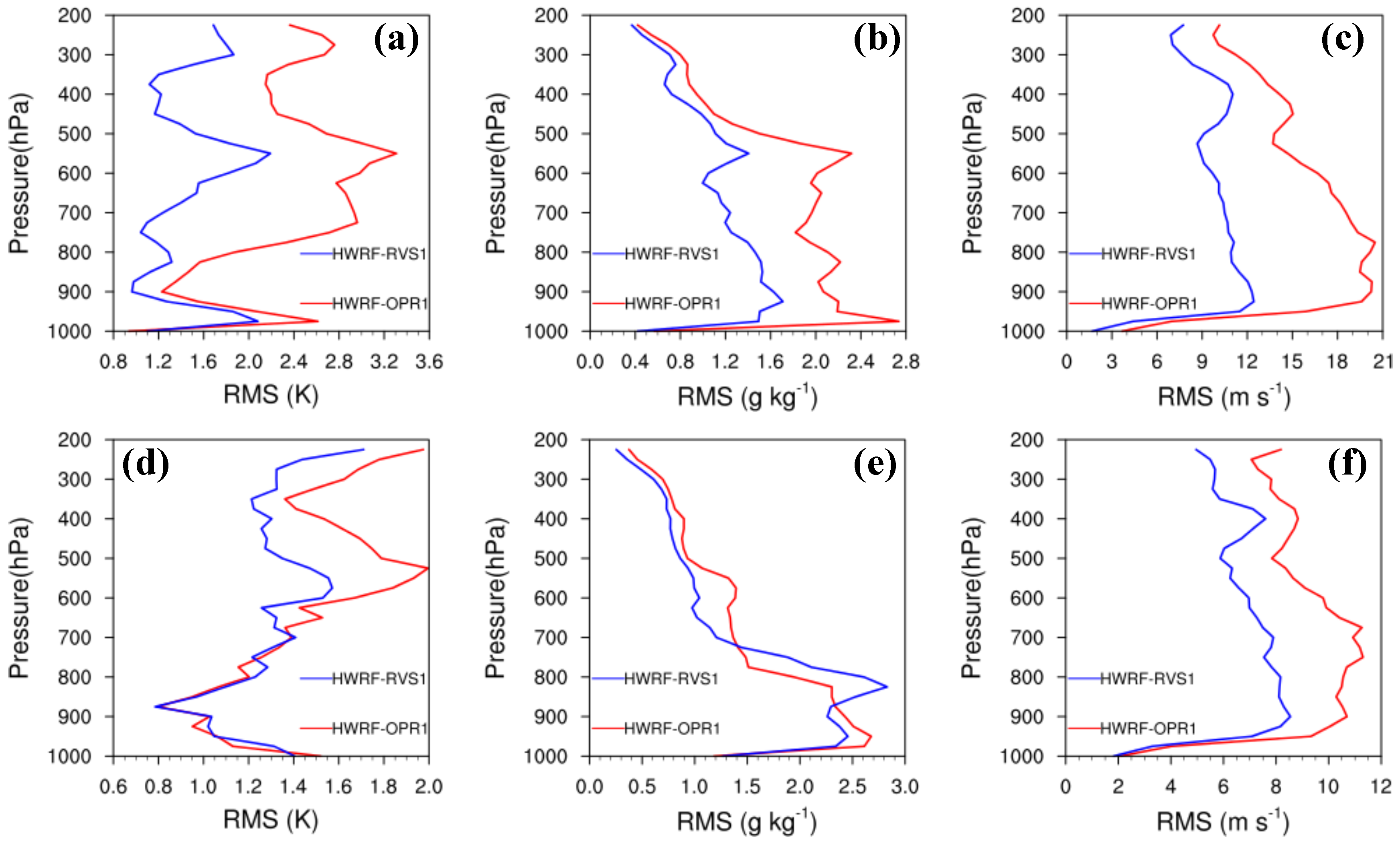
• Further diagnoses for Hurricane Joaquin indicate that 4DEnVar initialization framework, which does not use size and intensity correction in the vortex initialization, can significantly alleviate the gradient imbalances in the HWRF initial conditions produced by the operational initialization framework. In addition, 4DEnVar initialization framework can enhance the performance of DA, as it produces smaller HWRF analysis errors than the operational initialization framework does. This is because DA in 4DEnVar initialization framework not only involves the variation of the background error covariances within the DA window, but also uses high-resolution self-consistent HWRF ensembles that can provide detailed storm-scale features, which enhances the incorporation of observational information into the model initial conditions.
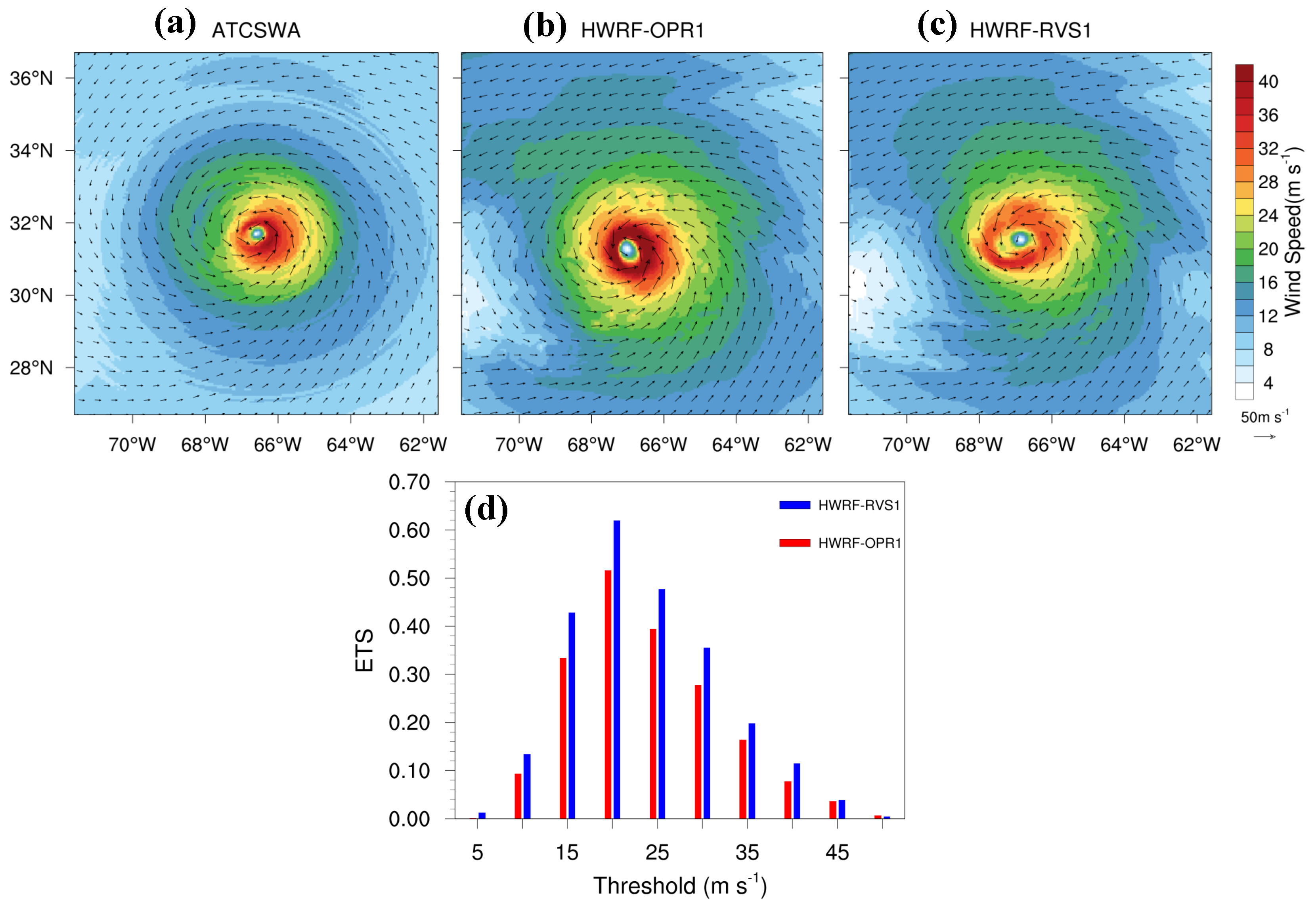
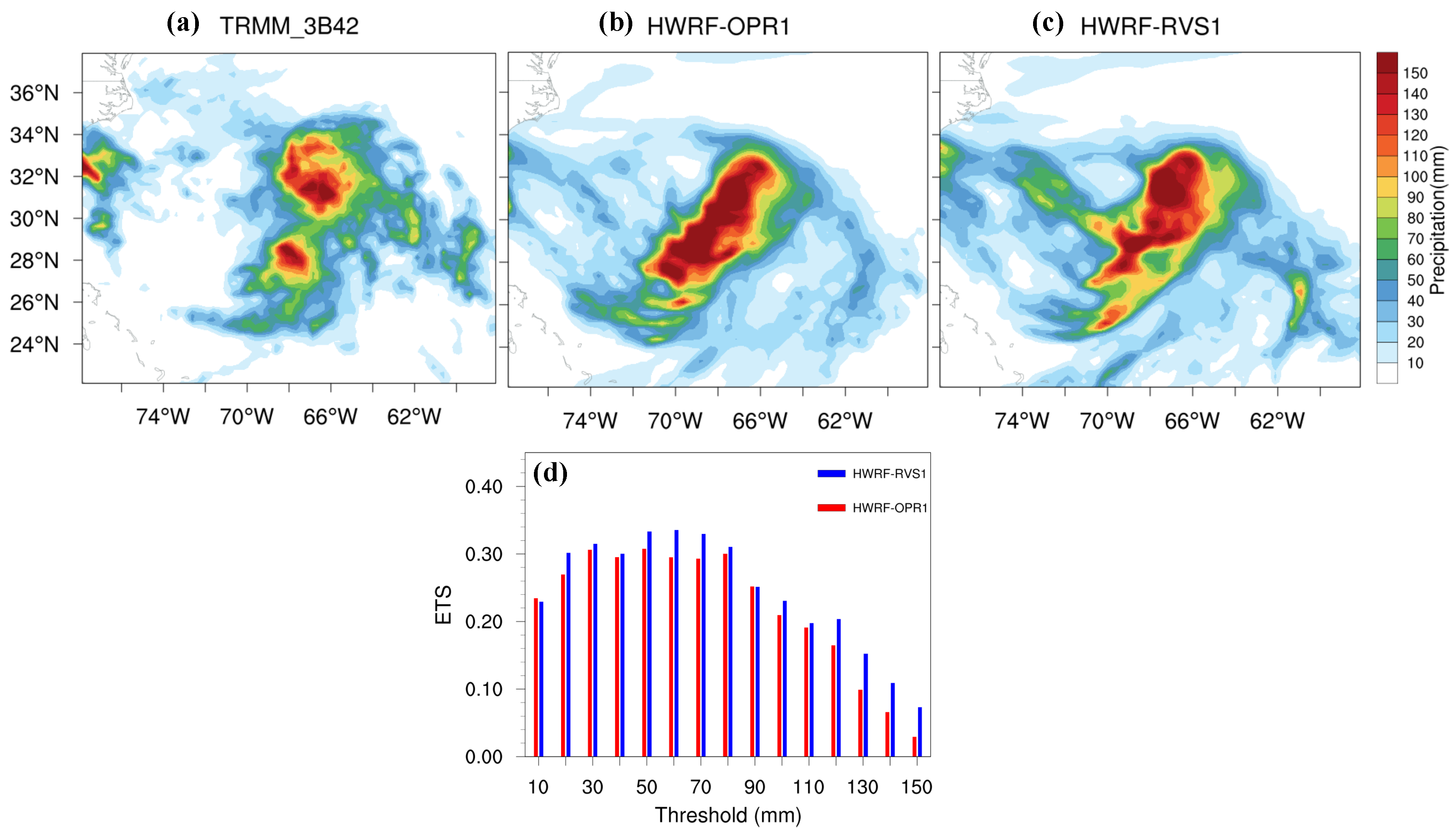
• The evaluation of the HWRF-forecasted 10-m wind and accumulated precipitation for Hurricane Joaquin shows that 4DEnVar initialization framework produces higher ETS scores for wind and precipitation during the intensity changes of Hurricane Joaquin than the operational initialization framework does. This indicates that 4DEnVar initialization framework also has the potential to improve quantitative wind and precipitation forecasts in HWRF.

Overall, the proposed initialization framework in this study reveals the potential to improve forecasts of TC intensity changes in HWRF. It suggests that the use of high-resolution self-consistent HWRF ensembles and the more advanced GSI-4DEnVar data assimilation systems can lead to noticeable improvements in the vortex initializations and forecasts of hurricanes using HWRF. Fortunately, advancing the DA system is of the utmost importance to improve hurricane forecasting models, like HWRF and its eventual successors [33]. In particular, the HWRF-based ensemble prediction system (EPS) has been implemented in operational TC forecasts in NCEP/EMC since 2014 [26], which provides strong support for the practical use of 4DEnVar initialization framework in the operational HWRF system. In addition, implementation of 4DEnVar in the NCEP global forecast system will make it possible to eventually move 4DEnVar into the HWRF DA system. We believe that our investigations in this study can provide useful guidance for future work. Furthermore, the new satellite-derived products such as enhanced AMVs and CYGNSS sea surface wind developed in current observational projects and TC field campaigns could be incorporated into 4DEnVar initialization framework to further improve hurricane initialization [17,19,34,35]. Finally, our evaluation in this study mainly focuses on the track and intensity forecasts for three selected hurricane cases during their rapid intensity changes. A larger sample of hurricane cases will be necessary to evaluate the consistency of the impacts on the HWRF Model provided by the revised initialization framework, and the detailed reasoning and physical understanding on the data assimilation results also need to be further discussed.

References

1. Elsberry, R.L. Achievement of USWRP Hurricane Landfall Research Goal. Bull. Am. Meteorol. Soc. 2005, 86, 643–646. [Google Scholar] [CrossRef]
2. Liu, J.; Zhang, F.; Pu, Z. Numerical simulation of the rapid intensification of Hurricane Katrina (2005): Sensitivity to boundary layer parameterization schemes. Adv. Atmos. Sci. 2017, 34, 482–496. [Google Scholar] [CrossRef]
3. Elsberry, R.L.; Lambert, T.D.B.; Boothe, M.A. Accuracy of Atlantic and Eastern North Pacific Tropical Cyclone Intensity Forecast Guidance. Weather Forecast. 2007, 22, 747–762. [Google Scholar] [CrossRef]
4. Zhang, F.; Weng, Y.; Gamache, J.F.; Marks, F.D. Performance of convection-permitting hurricane initialization and prediction during 2008? 2010 with ensemble data assimilation of inner-core airborne Doppler radar observations. Geophys. Res. Lett. 2011, 38. [Google Scholar] [CrossRef] [Green Version]
5. Rogers, R.; Aberson, S.; Aksoy, A.; Annane, B.; Black, M.; Cione, J.; Dorst, N.; Dunion, J.; Gamache, J.; Goldenberg, S.; et al. NOAA’S Hurricane Intensity Forecasting Experiment: A Progress Report. Bull. Am. Meteorol. Soc. 2013, 94, 859–882. [Google Scholar] [CrossRef] [Green Version]
6. DeMaria, M.; Mainelli, M.; Shay, L.K.; Knaff, J.A.; Kaplan, J. Further Improvements to the Statistical Hurricane Intensity Prediction Scheme (SHIPS). Weather Forecast. 2005, 20, 531–543. [Google Scholar] [CrossRef] [Green Version]
7. DeMaria, M.; DeMaria, R.T.; Knaff, J.A.; Molenar, D.A. Tropical Cyclone Lightning and Rapid Intensity Change. Mon. Weather Rev. 2012, 140, 1828–1842. [Google Scholar] [CrossRef]
8. National Hurricane Center Forecast Verification. 2017. Available online: https://www.nhc.noaa.gov/verification/verify5.shtml (accessed on 12 April 2019).
9. Pu, Z.; Zhang, S.; Tong, M.; Tallapragada, V. Influence of the Self-Consistent Regional Ensemble Background Error Covariance on Hurricane Inner-Core Data Assimilation with the GSI-Based Hybrid System for HWRF. J. Atmos. Sci. 2016, 73, 4911–4925. [Google Scholar] [CrossRef]
10. Hurricane Weather Research and Forecasting (HWRF) Model: 2015 Scientific Documentation. 2015. Available online: https://opensky.ucar.edu/islandora/object/technotes%3A535/datastream/PDF/download/citation.pdf (accessed on 22 March 2020).
11. Liu, Q.; Surgi, N.; Lord, S.; Wu, W.; Parrish, S.; Gopalakrishnan, S.; Waldrop, J.; Gamache, J. Hurricane Initialization in HWRF Model. Preprints. In Proceedings of the 27th Conference on Hurricanes and Tropical Meteorology, Monterey, CA, USA, 24–28 April 2006. [Google Scholar]
12. Wu, W.S.; Purser, R.J.; Parrish, D.F. Three-Dimensional Variational Analysis with Spatially Inhomogeneous Covariances. Mon. Weather Rev. 2002, 130, 2905–2916. [Google Scholar] [CrossRef] [Green Version]
13. Wang, X.; Parrish, D.; Kleist, D.; Whitaker, J. GSI 3DVar-Based Ensemble? Variational Hybrid Data Assimilation for NCEP Global Forecast System: Single-Resolution Experiments. Mon. Weather Rev. 2013, 141, 4098–4117. [Google Scholar] [CrossRef]
14. Lu, X.; Wang, X.; Li, Y.; Tong, M.; Ma, X. GSI-based ensemble-variational hybrid data assimilation for HWRF for hurricane initialization and prediction: Impact of various error covariances for airborne radar observation assimilation. Q. J. R. Meteorol. Soc. 2017, 143, 223–239. [Google Scholar] [CrossRef]
15. Tallapragada, V.; Kieu, C.; Kwon, Y.; Trahan, S.; Liu, Q.; Zhang, Z.; Kwon, I.H. Evaluation of Storm Structure from the Operational HWRF during 2012 Implementation. Mon. Weather Rev. 2014, 142, 4308–4325. [Google Scholar] [CrossRef]
16. Wang, X.; Lei, T. GSI-Based Four-Dimensional Ensemble?Variational (4DEnsVar) Data Assimilation: Formulation and Single-Resolution Experiments with Real Data for NCEP Global Forecast System. Mon. Weather Rev. 2014, 142, 3303–3325. [Google Scholar] [CrossRef]
17. Zhang, S.; Pu, Z.; Velden, C. Impact of Enhanced Atmospheric Motion Vectors on HWRF Hurricane Analyses and Forecasts with Different Data Assimilation Configurations. Mon. Weather Rev. 2018, 146, 1549–1569. [Google Scholar] [CrossRef]
18. Kleist, D.T.; Ide, K. An OSSE-Based Evaluation of Hybrid Variational?Ensemble Data Assimilation for the NCEP GFS. Part II: 4DEnVar and Hybrid Variants. Mon. Weather Rev. 2015, 143, 452–470. [Google Scholar] [CrossRef] [Green Version]
19. Zhang, S.; Pu, Z. Numerical Simulation of Rapid Weakening of Hurricane Joaquin with Assimilation of High-Definition Sounding System Dropsondes during the Tropical Cyclone Intensity Experiment: Comparison of Three- and Four-Dimensional Ensemble? Variational Data Assimilation. Weather Forecast. 2019, 34, 521–538. [Google Scholar] [CrossRef]
20. Gopalakrishnan, S.G.; Marks, F.; Zhang, X.; Bao, J.W.; Yeh, K.S.; Atlas, R. The Experimental HWRF System: A Study on the Influence of Horizontal Resolution on the Structure and Intensity Changes in Tropical Cyclones Using an Idealized Framework. Mon. Weather Rev. 2011, 139, 1762–1784. [Google Scholar] [CrossRef]
21. Janjic, Z.; Gall, Z.; Pyle, M.E. Scientific Documentation for the NMM Solver; (No. NCAR/TN-477+STR); National Center for Atmospheric Research University Corporation for Atmospheric Research: Boulder, CO, USA, 2010; 54p. [Google Scholar] [CrossRef]
22. Data Types Used by the GSI Analysis System. 2018. Available online: https://www.emc.ncep.noaa.gov/mmb/data_processing/prepbufr.doc/ (accessed on 12 April 2019).
23. Wang, X. Incorporating Ensemble Covariance in the Gridpoint Statistical Interpolation Variational Minimization: A Mathematical Framework. Mon. Weather Rev. 2010, 138, 2990–2995. [Google Scholar] [CrossRef] [Green Version]
24. Buehner, M.; Morneau, J.; Charette, C. Four-dimensional ensemble-variational data assimilation for global deterministic weather prediction. Nonlinear Process. Geophys. 2013, 20, 669–682. [Google Scholar] [CrossRef] [Green Version]
25. Lorenc, A.C.; Bowler, N.E.; Clayton, A.M.; Pring, S.R.; Fairbairn, D. Comparison of Hybrid-4DEnVar and Hybrid-4DVar Data Assimilation Methods for Global NWP. Mon. Weather Rev. 2015, 143, 212–229. [Google Scholar] [CrossRef]
26. Zhang, Z.; Tallapragada, V.; Kieu, C.; Trahan, S.; Wang, W. HWRF Based Ensemble Prediction System Using Perturbations from GEFS and Stochastic Convective Trigger Function. Trop. Cyclone Res. Rev. 2014, 3, 145–161. [Google Scholar] [CrossRef]
27. Berg, R. National Hurricane Center Tropical Cyclone Report, Hurricane Joaquin (AL112015). NOAA/National Hurricane Center, 2016; 36p. Available online: https://www.nhc.noaa.gov/data/tcr/AL112015_Joaquin.pdf (accessed on 12 April 2019).
28. Knaff, J.A.; Longmore, S.P.; DeMaria, R.T.; Molenar, D.A. Tropical Cyclone Lightning and Rapid Intensity Change. J. Appl. Meteor. Climatol. 2015, 54, 463–478. [Google Scholar] [CrossRef] [Green Version]
29. Knaff, J.A.; Zehr, R.M. Reexamination of tropical cyclone wind—Pressure relationships. Weather Forecast. 2007, 22, 71–88. [Google Scholar] [CrossRef]
30. ONR Tropical Cyclone Intensity 2015 NASA WB-57 HDSS Dropsonde Data. 2016. Available online: https://data.eol.ucar.edu/dataset/488.004 (accessed on 12 April 2019).
31. Kimberlain, T.; Blake, E.; Cangialosi, J. National Hurricane Center Tropical Cyclone Report, Hurricane Patricia (EP202015). NOAA/National Hurricane Center, 2016; 32p. Available online: https://www.nhc.noaa.gov/data/tcr/EP202015_Patricia.pdf (accessed on 12 April 2019).
32. Stewart, S. National Hurricane Center Tropical Cyclone Report, Hurricane Matthew (AL142016). NOAA/National Hurricane Center, 2017; 96p. Available online: https://www.nhc.noaa.gov/data/tcr/AL142016_Matthew.pdf (accessed on 12 April 2019).
33. Hurricane Weather Research and Forecasting (HWRF) Model: 2018 Scientific Documentation. 2018. Available online: https://dtcenter.org/sites/default/files/community-code/hwrf/docs/scientific_documents/HWRFv4.0a_ScientificDoc.pdf (accessed on 22 March 2020).
34. Cui, Z.; Pu, Z.; Tallapragada, V.; Atlas, R.; Ruf, C.S. A Preliminary Impact Study of CYGNSS Ocean Surface Wind Speeds on Numerical Simulations of Hurricanes. Geophys. Res. Lett. 2019, 46, 2984–2992. [Google Scholar] [CrossRef] [PubMed] [Green Version]
35. Lu, X.; Wang, X. Improving Hurricane Analyses and Predictions with TCI, IFEX Field Campaign Observations, and CIMSS AMVs Using the Advanced Hybrid Data Assimilation System for HWRF. Part II: Observation Impacts on the Analysis and Prediction of Patricia (2015). Mon. Weather Rev. 2020, 148, 1407–1430. [Google Scholar] [CrossRef]
Figure 1. Flow charts for the HWRF simulations based on (a) the 3DEnVar initialization framework and (b) 4DEnVar initialization framework.
Atmosphere 11 01007 g001
Figure 2. (a) Forecast domains, as indicated by d01, d02, and d03, and HWRF data assimilation domains, as indicated by ghost d02 (black shaded area), and ghost d03 (pink shaded area) for the 3DEnVar initialization framework; and (b) forecast domains and data assimilation domains as indicated by d01, d02 and d03 for 4DEnVar initialization framework. Data assimilation in the 4DEnVar initialization framework is directly performed on d02 and d03. The black symbol indicates the storm center from National Hurricane Center (NHC) best track (black storm sign).
Atmosphere 11 01007 g002
Figure 3. Radius–height cross sections of the isopleths of net radial force per unit mass (unit: m s 1 h 1 ). The top four panels show the results from HWRF-OPR1 that are diagnosed (a) before vortex initialization (VI), (b) after VI, (c) after data assimilation (i.e., analysis) and (d) 3-h forecast at the analysis cycle of 1800 UTC 03 October 2015. The bottom four panels represent the results from HWRF-REV1 that are diagnosed (e) before VI, (f) after VI, (g) after data assimilation (i.e., analysis) and (h) 3-h forecast at the analysis cycle of 1800 UTC 03 October 2015. The contour interval is 20 m s 1 h 1 , with dashed lines indicating negative values. The zero contour is not plotted. The red lines indicate the radius of maximum wind. We note that the VI in HWRF-OPR1 enables both the vortex relocation and intensity correction, while VI in HWRF-REV1 only enables the vortex relocation, as shown in Table 1.
Atmosphere 11 01007 g003
Figure 4. The root-mean-square (RMS) fit of the analysis to in situ observations within d02 region (Table 1) averaged over the data assimilation period from 1800 UTC 02 to 1800 UTC 03 October 2015 for (a) temperature and (b) wind as a function of pressure. (c) the RMS fit of the analyzed wind to in situ observations within d03 from 1000 hPa to 500 hPa during the data assimilation period from 1800 UTC 02 to 1800 UTC 03 October 2015. Red lines indicate the results from HWRF-OPR1, and blue lines indicate the results from HWRF-RVS1.
Atmosphere 11 01007 g004
Figure 5. Vertical distribution of observations that are assimilated by Gridpoint Statistical Interpolation (GSI) for Hurricane Joaquin at (a) 1800 UTC 2 October 2015 and (b) 1800 UTC 3 October 2015. The large orange dots denote the temperature (t) and humidity (q) data; while the small blue dots represent wind data (u and v). The numbers of observations that are assimilated in three different levels (below 750 hPa, 500–750 hPa, and 200–500 hPa) are also shown on the top of (a) and (b). The x-axis represents the distance to the storm center.
Atmosphere 11 01007 g005
Figure 6. Ensemble spreads of temperature (unit: °C) at 850 hPa within 6-h analysis window (−3 h–3 h) around 1800 UTC 03 October 2015 from (a) National Centers for Environmental Prediction (NCEP) Global Forecast System (GFS) ensemble Kalman filtering (EnKF) 80-member ensemble forecasts at ∼23 km horizontal resolution and (bh) HWRF 42-member ensemble forecasts at 6 km horizontal resolution. The numbers in each plot indicate the differences between the ensemble forecast time and the analysis time.
Atmosphere 11 01007 g006
Figure 7. Vortex structure of Hurricane Joaquin at 1800 UTC 03 October 2015 as revealed by wind speed (shaded; unit: m s 1 ) and vectors at 10-m height from (a) Aircraft-based Tropical Cyclone Surface Wind Analysis (ATCSWA), (b) HWRF-OPR1 and (c) HWRF-RVS1.
Atmosphere 11 01007 g007
Figure 8. The RMS fit of the forecasts to the dropsonde observations for (left) temperature ( K ), (middle) specific humidity ( g kg 1 ) and (right) wind speed ( m s 1 ) as a function of pressure at (ac) 24-h and (df) 48-h forecast lead times for the experiments of HWRF-OPR1 (red lines) and HWRF-RVS1 (blue lines).
Atmosphere 11 01007 g008
Figure 9. Time series (at 6-h intervals) of (a) track, (b) minimum sea level pressure (MSLP, hPa) and (c) maximum surface winds (MSW, m s 1 ) for Hurricane Joaquin during 1800 UTC 03–1800 UTC 06 October 2015. The colored numbers on the top of figures represent the average track (a), MSLP (b) and MSW (c) errors over the whole 72-h forecast period.
Atmosphere 11 01007 g009
Figure 10. Vortex structure of Hurricane Joaquin at 1800 UTC 04 October 2015 as revealed by wind speeds (shaded; unit: m s 1 ) and vectors at 10 m height from (a) ATCSWA, (b) HWRF-OPR and (c) HWRF-RVS1. (d) the mean equitable threat score (ETS) of the 10-m forecasted wind field from HWRF-OPR1 (red bars) and HWRF-RVS1 (blue bars) compared against the 10-m wind analysis from ATCSWA with thresholds of 5, 10, 15, 20, 25, 30, 35, 40, 45 and 50 m s 1 . The mean ETS is calculated during the rapid weakening of Hurricane Joaquin from 1800 UTC 03 to 0000 UTC 05 October 2015 with a 6-h interval.
Atmosphere 11 01007 g010
Figure 11. Accumulated precipitation (unit: mm) from (a) Tropical Rainfall Measuring Mission (TRMM) 3B42, (b) HWRF-OPR1 and (c) HWRF-RVS1 during the rapid weakening of Hurricane Joaquin from 1800 UTC 03 to 0000 UTC 05 October 2015. (d) The equitable threat score (ETS) of the 30-h accumulated precipitation from HWRF-OPR1 (red bars) and HWRF-RVS1 (blue bars) compared against TRMM 3B42 precipitation observations with thresholds of 10, 20, 30, 40, 50, 60, 70, 80, 90, 100, 110, 120, 130, 140 and 150 mm.
Atmosphere 11 01007 g011
Figure 12. Time series (at 6-h intervals) of (a) track, (b) minimum sea level pressure (MSLP, hPa) and (c) maximum surface wind (MSW, m s 1 ) for Hurricane Patricia during 1800 UTC 21–1200 UTC 24 October. The colored numbers on the top of figures represent the average track (a), MSLP (b) and MSW (c) errors over the first 24-h forecast period.
Atmosphere 11 01007 g012
Figure 13. Time series (at 6-h intervals) of (a) track, (b) minimum sea level pressure (MSLP, hPa) and (c) maximum surface wind (MSW, m s 1 ) for Hurricane Matthew during 1800 UTC 29 September–1800 UTC 02 October 2016. The colored numbers on the top of figures represent the average track (a), MSLP (b) and MSW (c) errors over the first 24-h forecast period.
Atmosphere 11 01007 g013