Article

An Improved Method for Optical Characterization of Mineral Dust and Soot Particles in the El Paso-Juárez Airshed

1
Departamento de Física y Matemáticas, Universidad Autónoma de Ciudad Juárez, Avenida del Charro #450 N, Ciudad Juárez, Chihuahua 32310, Mexico
2
Department of Physics, University of Texas at El Paso, 500 W. University Ave., El Paso, TX 79968, USA
*
Author to whom correspondence should be addressed.
Atmosphere 2020, 11(8), 866; https://doi.org/10.3390/atmos11080866
Submission received: 7 July 2020 / Revised: 11 August 2020 / Accepted: 13 August 2020 / Published: 15 August 2020
(This article belongs to the Special Issue Atmospheric Aerosols in North America)

Abstract

:
Highly time-resolved aerosol measurements and analysis are necessary for a proper aerosol characterization in many polluted regions, because aerosol concentrations in polluted environments can change over time scales of minutes. However, many urban measuring sites have measuring devices that provide time resolved average aerosol concentrations over a day or two at best. Light-scattering properties of mineral dust and soot particles in the El Paso-Juárez Airshed were analyzed with an improved methodology, using the T-matrix, a maximum likelihood estimator (MLE), and data from both an acoustic extinctiometer and a laser particle counter. The hourly inter-comparisons of the scattering coefficients’ results between the model and those obtained using the instruments at a wavelength of 0.87 μm show good agreement. This methodology has been applied in the El Paso-Juárez Airshed successfully, and it could be used in other cities where mineral dust and soot are major components of the aerosol concentrations.

1. Introduction

Medina et al. [1] developed a novel methodology to characterize the optical properties of mineral dust and soot particles, that was based on T-matrix theory [2]. The T-matrix model was used to calculate the scattering and extinction cross sections for the aerosols present in the El Paso-Juarez Airshed. The T-matrix theory was selected because it could be applied to randomly oriented, non-spherical rotational symmetric particles. The study inter-compared daily mean scattering coefficients through the analysis of data from an acoustic extinctiometer and a laser particle counter, in conjunction with a non-spherical scattering model, the T-matrix that was used to obtain the scattering coefficients. The comparisons of the calculated values with data showed that the agreement was good. In this research, using mathematical models, we have improved, made more accurate and highly time-resolved the cited publication, as discussed in Section 2.
Mineral dust has important climate effects due to its scattering of atmospheric radiation and its role in cloud formation [3,4,5,6,7]. Soot harms human health [8,9,10], while the effects of mineral dust on human health are less clear [11]; however, there is more recent evidence that mineral dust causes cardiopulmonary disease and lung cancer, leading to premature death [12].
Atmospheric concentrations of mineral dust in desert regions are largely determined by prevailing wind speeds and surface vegetation [3]. The size distribution of desert dust aerosols is an important quantity because it affects the impact of these aerosols on climate [13], with the Saharan dust being an important example [14].
Soot is another major focus of this paper, but elemental carbon, soot and brown carbon have to be separately distinguished [15]. Elemental carbon and soot are emitted from high temperature combustion sources, and both strongly absorb atmospheric radiation across the spectrum from the ultraviolet through the infrared, and this absorbance of atmospheric radiation may have significant climate effects [16]. Elemental carbon is refractory and does not volatilize below ~400 °C in air [16,17]. Soot is emitted from high temperature combustion sources, but soot is not a single compound; rather, it is composed of elemental carbon and other carbonaceous material that incorporates trace amounts of hydrogen, nitrogen, oxygen and other elements [16]. Brown carbon is a product of low-temperature combustion of organic material, and it is a major component of brown smoke. Brown carbon is composed of organic compounds, including alcohols, aromatics, di/tri organic acids, hydroxyacids, ketoacids and sugars [15,16,17]. The impact of mineral dust and soot on human health and climate make new methods for the analysis of the optical properties of these aerosols very relevant [18,19,20,21]. In El Paso, Texas aerosols consisting of mineral dust and soot are very common, as can be seen in Figure 1, on the left. The main component of mineral dust for this region is silica (SiO2), which was verified by EDS (energy dispersive X-ray spectroscopy).
The city of El Paso, Texas is located near the western tip of the state of Texas. El Paso has a population of over 680,000, and it shares a border region with Ciudad Juárez, Mexico, which has around 1.4 million inhabitants, and El Paso is adjacent to Las Cruces, New Mexico. The El Paso-Juárez urban region is among the largest bi-national metropolitan areas in the world, one of the fifty largest metropolitan areas in the Western Hemisphere, and it is technically isolated, centered in a radius of 500 km between the nearest urban areas with similar size, including San Antonio, Austin, Albuquerque and Chihuahua City. This relative isolation of the El Paso-Juárez region makes it an ideal site for air quality studies of isolated urban environments that are potentially affected by soot emissions within an airshed, as shown in Figure 1 Right. Furthermore, this region is located in the heart of the Chihuahua Desert (an area of 362,000 km2), which is otherwise sparsely populated. The region has a complex mountain-desert topography with a river valley area. This results in a constrained air basin where anthropogenic air pollution could be trapped over the metropolitan area, mainly during summer and winter seasons. In the El Paso-Juárez Airshed, mineral-dust and soot are the predominant components of atmospheric aerosols, as reported by Esparza et al. 2011 [21] and Pearson et al. [22] Sandstorms, windy days that occur during winter and early spring with winds striking up to 63 km/h with peak record of 135 km/h, blow mineral dust and sand out of the surrounding desert, causing high particulate concentrations [23]. In addition, these high wind dust events reduce visibility, and are a major concern for the health of the residents in the El Paso-Juarez airshed.
One major source of soot in the metropolitan area is attributed to local anthropogenic sources such as automobile emissions, three international ports of entry from Ciudad Juárez, México, El Paso, TX, US and Santa Teresa, NM, US, as described by Chen et al. 2012 [24]. These considerations make aerosol observations in the El Paso-Juárez Airshed valuable for testing mathematical models that could potentially advance the understanding of mineral dust and soot aerosols. Characterization of optical properties are essential to assess the radiative aerosol effect and their atmospheric climate impact.
In 2018, Medina et al. [1] outlined future work involving the development of increased accuracy and the application of the new methodology to the investigation of the optical properties of aerosol particles. In this work, we present an improved method based on hourly inter-comparisons of scattering coefficients, to provide a highly time-resolved methodology needed to provide a high-standard approximation and correlation of observations of aerosol airshed loading, which can change within minutes or less of time.

2. Methodology

2.1. Instruments

We used a CI-150t Climet (Climet:, Redlands, CA, US) and extinctiometer photoacoustic extinctiometer (PAX) instruments (Droplet Measurement Technologies: Boulder, CO, US) [25,26,27], which allow us to obtain the scattering coefficients (i.e., a measure of the ability of particles to scatter photons out of a beam of light) and the number of particles per unit volume at different radii intervals.
PAX stands for photoacoustic extinctiometer. We use this instrument to measure the black and brown carbon concentration in the El Paso airshed. Our objective is to register these concentrations where the sources are wildfires, either regionally or out of the area occurrences. The main characteristic of this instrument is its dual function: recording the portion of the electromagnetic incident wave that gets scattered, and the portion that gets absorbed. A minimal 1 L/min aerosol sample is collected into the PAX through an internal vacuum pump controlled by two critical orifices. The PAX uses a wide-angle integrating reciprocal nephelometer to measure the light scattering coefficient. The scattering measurement responds to all particle types, regardless of chemical makeup, mixing state, or morphology. The air sample is divided between the nephelometer and photoacoustic resonator for simultaneous measurement of light scattering and absorption. For the photoacoustic portion, in the laser chamber, the particles absorb the laser’s light, which causes local heating and thermoelastic expansion. Pressure or soundwaves are emitted and detected by an ultra-high frequency transducer. These signals are then processed and analyzed to determine the coefficients.
The CLiMET, CI-150t model is a particle counter instrument. With a flow of 1 cubic foot per minute (CFM), and a delay in between samples of 15 min, the instrument “counts” the number of particles as they flow through is internal chamber, and then displays the amount of particles by diameter size, in micrometers. This particle counter is a laser diode-based aerosol particle counter that monitors particles in four size ranges: 0.3, 0.5, 1.0, and 5.0, or larger micrometer particles, and contains an internal HEPA filtered exhaust (RS-232) (Honeywell: Canton, MA, US). These numbers are the upper limit for the diameter size, but in here, we will consider radius size from now on. Up to 3000 samples can be stored in the Climet’s internal memory, and can be transferred as a comma delimited ASCII file through the RS-232 serial port to a computer. They can also be easily transferred to common spreadsheets. All samples are date and time stamped.
The radii intervals are referred to as bins in this paper. In Figure 2, it is possible to observe the heights of each bin (the last one being truncated to 10 microns), so that the area underneath represents the number of particles per unit volume over the range of each bin. As the number density is more concentrated in the smallest bin and sparse in the largest bin, a log-log scale is presented. The ranges per bin are as follows: bin 1 = [0.15, 0.25], bin 2 = [0.25, 0.5], bin 3 = [0.5, 2.5], and bin 4 = [2.5, 10]; units are in microns. As both instruments measure data at different time intervals, averaging is necessary to match instances of time. Specifically, the PAX instrument provides measurements that are 6 minute-averages, with the reported time corresponding to 3 min. This averaging has some impact on data fitting and can cause some removable data discontinuities.
The scattering coefficients (B), scattering cross sections (C), and number of particles (N) are related by
B = CN.
The PAX instrument provides the scattering coefficients B, while the Climet instrument gives the number of particles per unit volume per bin. Scattering cross sections are needed, so they can be computed via the T-matrix approach using a computer code developed by Mishchenko et al. [2]
As the number of particles are obtained from the CI-150t Climet® per bin [21], we assume a lognormal distribution of particle size; however, the mean and standard deviation need to be calculated. For this purpose, the maximum likelihood estimator is used, which in turn is based on Newton’s method to minimize the error in evaluating these parameters, as described in the next subsections.

2.2. Models

2.2.1. Maximum Likelihood Estimator (MLE)

Maximum likelihood estimation (MLE) is a technique used for estimating the parameters of a given distribution, using some observed data.
As a formal definition: let Y 1 , Y 2 , ,   Y n be observations from n independent and identically distributed random variables, drawn from a probability distribution f 0 , where f 0 is known to be from a family of distributions f that depend on some parameters θ . The goal of MLE is to maximize the likelihood function:
L = f ( Y 1 , Y 2 , ,   Y n | θ ) = f ( Y 1 | θ ) × × f ( Y n | θ ) .
The multiplication principle of these probabilities means that we have the intersection of them happening simultaneously. Often, the log-likelihood function is easier to work with:
l ^ = l n   L =   i = 1 n l n   f ( x i | θ )
Let [ a i ,   b i ) (Einstein’s notation) be a partition function of [0, ∞). In our context, the intervals [ a i ,   b i ) correspond to the bins. The probability that a value Y drawn from a lognormal distribution with logarithmic mean μ and logarithmic standard deviation σ lies in the interval [ a i ,   b i ) therefore is
f i ( μ , σ ) = P ( a i Y < b i ) = Φ [ l n ( b i ) μ σ ] Φ [ l n ( a i ) μ σ ] ,
where Φ(x) is the cumulative canonical normal distribution.
When the data consist of independent draws Y 1 , Y 2 , ,   Y N , with Y j falling in bin i ( j ) and the bin cutpoints are established independently of the Y j , the probabilities multiply, hence the logarithmic likelihood is the sum of the logarithms of the values f i ( j ) ( μ ,   σ ) .
It suffices to count the number of Y j falling with each bin i ; let this count be k ( i ) . By collecting the k ( i ) terms associated with bin i for each bin, the sum condenses to
g ( μ ,   σ ) = k i l n   f i ( μ ,   σ ) ,
where the k i = k ( i ) are the weights at each interval [ a i ,   b i ) . We seek optimum values μ ^ and σ ^ . Starting with “good” values μ 0 and σ 0 , one way to find an extremum (assuming it is not a saddle point) would be to use Newton–Raphson’s method, which finds updated values of μ and σ by solving the linear system of equations at each step, with iterations converging, as described by:
[ 2 g μ 2 2 g μ σ 2 g σ μ 2 g σ 2 ] [ Δ μ Δ σ ] = [ g μ g σ ] .
To simplify the notation, we introduce new variables v i and u i for the arguments of ϕ :
v i = ln b i μ σ ,   u i = ln a i μ σ
then, the first partial derivatives (Appendix A) are:
g μ = k i σ f i [ ϕ ( v i ) ϕ ( u i ) ]
and
g σ = k i σ f i [ v i ϕ ( v i ) u i ϕ ( u i ) ] ,
where Φ = ϕ ; the second partial derivatives (Appendix A) are:
2 g μ 2 = k i σ 2 f i 2 { f i [ v i ϕ ( v i ) u i ϕ ( u i ) ] + [ ϕ ( v i ) ϕ ( u i ) ] 2 } ,
2 g μ σ = 2 g σ μ = k i σ 2 f i 2 { f i 2 [ v i 2 ϕ ( v i ) u i 2 ϕ ( u i ) ] + [ ϕ ( v i ) ϕ ( u i ) ] [ v i ϕ ( v i ) u i ϕ ( u i ) f i ] } ,
and
2 g σ 2 = k i σ 2 f i 2 { [ v i ϕ ( v i ) u i ϕ ( u i ) ] [ v i ϕ ( v i ) u i ϕ ( u i ) 2 f i ] + f i [ v i 3 ϕ ( v i ) u i 3 ϕ ( u i ) ] .

2.2.2. Bi-Modal Distribution

In our theoretical model for distinction between particles, we assume soot to be majorly present on bins for small particle sizes; and in case of larger size bins mineral dust is assumed to be present. For the second bin, which is in the middle of what are considered small and large radii, both soot and mineral dust exist mixed at different percentages, so we set them to add up to 100%, going from one extreme (100% soot, 0% mineral dust) to the other extreme (0% soot, 100% mineral dust), in steps of 1%.

2.2.3. T-matrix Code

Once the parameters are obtained for the bi-modal distribution, these are used as input data in the T-matrix code developed by Mishchenko et al. [2], which is separately applied in two modes, for soot (refractive index n = 1.75 + 0.43 i ) [28] and for mineral dust (refractive index n = 1.53 + 0.008 i ) [29], to achieve a numerical computation of optical cross sections, as described by:
C s c a t = r 1 r 2 C s c a t ( r ) n ( r ) d r ,
where r 1 and r 2 correspond to lower and upper radii for each bin. In particular, for the second bin ( 0.25   μ m < r < 0.5   μ m ), the corresponding integral splits into two integrals, one for soot and another one for mineral dust:
C s c a t = ( S o o t ) r 1 r 2 C s c a t ( r ) n ( r ) d r + ( M i n e r a l   D u s t ) r 1 r 2 C s c a t ( r ) n ( r ) d r .
It is assumed that the upper limit for the rightmost bin is truncated to 10 microns, where the size distribution function n ( r ) is negligible. Each integral is calculated using Gaussian quadrature, where the intervals are partitioned into subintervals; the partition and degree of the quadrature are adjusted to reduce the round-off error up to an acceptable numerical accuracy ϵ .

2.2.4. The Scattering Coefficients

The scattering coefficients can be obtained as:
B = N 1 C 1 + N 2 C 2 + N 3 C 3 + N 4 C 4 ,
where B, the scattering coefficient, can also be measured using the PAX extinctiometer; N j is the number of aerosol particles per unit volume on bin j and C j is the scattering cross section, also on bin j, obtained using the T-matrix model.

3. Results and Discussion

We present, in this work, three representative days with dates in year 2013: 22 March, 13 April, and 23 April. On Figure 3, Figure 4 and Figure 5, the models’ normalized results in magenta correspond to NC/(NC)max and the PAX instrument’s normalized results in blue correspond to B/Bmax, according to Equation (1). As observed, the Pearson correlation coefficient is greater than 0.93, 0.97, and 0.86, respectively. Features like extrema and concavity are in agreement between the experimental data and the theoretical model, as presented in Figure 3, Figure 4 and Figure 5. The higher correlation value occurred during 13 April 2013, with a Pearson Coefficient of 0.9775.
From Table 1, the mixture amount assumed for the second bins leading to the maximum Pearson correlation coefficient per date are as follows: 03/22/13 Soot: 57%; Mineral Dust: 43%, (r = 0.96637). 13 April 2013, Soot: 11%; Mineral Dust: 89% (r = 0.9775). 23 April 2013: Soot: 25%; Mineral Dust: 75% (r = 0.86424).
When performing these types of studies, hysplit backward trajectories have also been successfully used to identify the aerosol hotspots [30].
We observe that, on 22 March, we had the day of greatest concentration of soot, whereas 13 April had the greatest concentration of mineral dust. Figure 6 shows the backward trajectories for 22 March, the air masses move closer to the ground through the desert and the urban city of Juarez, therefore observing more soot aerosols. Figure 7 shows the Backward trajectories for 13 April, going more through the desert region and avoiding the city of Juarez. 23 April also had a great concentration of mineral dust, and some soot, consistent with Figure 8, the backward trajectory for that day, with the air masses going through the desert and the city of Juarez and then moving upwards in the atmosphere.

4. Conclusions

We found that aerosol scattering was the most significant contributing factor to atmospheric extinction. However, as expected, soot contributed most strongly to extinction by absorption.
Our theoretical and experimental analysis found a higher concentration of smaller size particles present in the El Paso-Juarez Airshed.
On 13 April and 23 April, it was observed there was a smaller concentration of soot, in comparison with 22 March, consistent with the Hysplit air masses Backward Trajectories path.
An improved method for optical characterization of mineral dust and soot particles has been successfully derived and applied to the El Paso-Juarez Airshed.
The inter-comparisons between the model’s scattering coefficients and the corresponding experimental data were excellent, with Pearson correlation coefficients of 0.93, 0.97, and 0.86.
Therefore, we conclude that our method is a valuable low cost and feasible method to estimate highly time-resolved aerosol concentrations over the El Paso-Juárez region and has great potential to be applied elsewhere.

Author Contributions

Conceptualization, J.P. and R.M.F.; Funding acquisition, R.M.F.; Methodology, J.P. and R.M.F.; Supervision, R.M.F. and W.R.S.; Writing—original draft, J.P.; Writing—review and editing, M.R., R.M.F. and W.R.S. All authors have read and agreed to the published version of the manuscript.

Funding

This research was funded by the NOAA Center for Atmospheric Science and Meteorology (NCASM), which is funded by the National Atmospheric Administration/Educational Partnership Program under Cooperative Agreement #NA16SEC4810006.

Acknowledgments

The first author would like to thank the Department of Physics at The University of Texas at El Paso for usage of the laboratory and computational cluster, the Consejo Nacional de Ciencia y Tecnología-México for Sistema Nacional de Investigadores Fellowship and to Universidad Autónoma de Ciudad Juárez.

Conflicts of Interest

The authors declare no conflict of interest. The funders had no role in the design of the study; in the collection, analyses, or interpretation of data; in the writing of the manuscript, or in the decision to publish the results.

Appendix A. Partial Derivatives

First Partial Derivatives
We start from the objective function to be maximized:
g ( μ ,   σ ) = k i l n f i ( μ ,   σ ) ,
where
f i ( μ , σ ) = Φ [ l n ( b i ) μ σ ] Φ [ l n ( a i ) μ σ ] ,
where Φ = ϕ . Let us define v i and u i as
v i = ln   b i μ σ ,   u i = ln a i μ σ .
The corresponding total differentials are obtained:
d g = k i d ( ln   f i ) =   k i f i d f i ,
d f i =   Φ ( v i ) d v i   Φ ( u i ) d u i ,
d v i =   1 σ ( d μ + v i d σ ) ,
and
d u i =   1 σ ( d μ + u i d σ ) .
Going backwards, we get more elaborated formulae:
d f i =   1 σ { [ ϕ ( v i )   ϕ ( u i ) ] d μ + [ v i ϕ ( v i )   u i ϕ ( u i ) ] d σ } ,
i.e.,
d g =   k i σ f i { [ ϕ ( v i )   ϕ ( u i ) ] d μ + [ v i ϕ ( v i )   u i ϕ ( u i ) ] d σ } .
The first partial derivatives readily follow:
g μ =   k i σ f i [ ϕ ( v i )   ϕ ( u i ) ]
and
g σ =   k i σ f i [ v i ϕ ( v i )   u i ϕ ( u i ) ] .
Second Partial Derivatives
To find the second partial derivatives, we need a chain of results:
d [ σ f i ] 1 = σ 1 d ( f i 1 ) +   f i 1 d ( σ 1 ) ,
d ( f i 1 ) =   d f i f i 2 =   1 σ { [ ϕ ( v i )   ϕ ( u i ) ] d μ + [ v i ϕ ( v i )   u i ϕ ( u i ) ] d σ } ,
d ( σ 1 ) =   1 σ 2 d σ ,
then
d [ σ f i ] 1 =   1 σ 2 f i 2 { [ ϕ ( v i )   ϕ ( u i ) ] d μ + [ v i ϕ ( v i )   u i ϕ ( u i ) f i ] d σ } .
Furthermore,
d [ ϕ ( v i )   ϕ ( u i ) ] =   1 σ { [ v i ϕ ( v i ) u i ϕ ( u i ) ] d μ + [ v i 2 ϕ ( v i ) u i 2 ϕ ( u i ) ] d σ }
and
d [ v i ϕ ( v i )   u i ϕ ( u i ) ] = 1 σ { [ ( 1 v i 2 ) ϕ ( v i )   ( 1 u i 2 ) ϕ ( u i ) ] d μ + [ ( 1 v i 2 ) v i ϕ ( v i )   ( 1 u i 2 ) u i ϕ ( u i ) ] d σ } .
All these results are needed into the product rules before computing the second order derivatives:
d { 1 σ f i [ ϕ ( v i )   ϕ ( u i ) ] } =   1 σ f i d [ ϕ ( v i )   ϕ ( u i ) ] + [ ϕ ( v i )   ϕ ( u i ) ] d [ σ f i ] 1
and
d { 1 σ f i [ v i ϕ ( v i )   u i ϕ ( u i ) ] } =   1 σ f i d [ v i ϕ ( v i )   u i ϕ ( u i ) ] + [ v i ϕ ( v i )   u i ϕ ( u i ) ] d [ σ f i ] 1 .
From the first product rule, two second order derivatives are derived:
2 g d μ 2 =   k i σ 2 f i 2 { f i [ v i ϕ ( v i )   u i ϕ ( u i ) ] + [ ϕ ( v i )   ϕ ( u i ) ] 2 } ,
2 g σ μ =   k i σ 2 f i 2 { f i [ v i 2 ϕ ( v i )   u i 2 ϕ ( u i ) ] + [ ϕ ( v i )   ϕ ( u i ) ] [ v i ϕ ( v i )   u i ϕ ( u i ) f i ] } .
From the second product rule, the other two second order derivatives are derived:
2 g μ σ =   k i σ 2 f i 2 { [ v i ϕ ( v i )   u i ϕ ( u i ) ] [ ϕ ( v i )   ϕ ( u i ) ] f i [ ( 1 v i 2 ) ϕ ( v i )   ( 1 u i 2 ) ϕ ( u i ) ] } ,
2 g σ 2 =   k i σ 2 f i 2 { [ v i ϕ ( v i )   u i ϕ ( u i ) ] [ v i ϕ ( v i )   u i ϕ ( u i ) f i ] f i [ ( 1 v i 2 ) v i ϕ ( v i )   ( 1 u i 2 ) u i ϕ ( u i ) ] } .
Although the cross derivatives look different, it can be shown that they are equivalent. In a similar manner, after some arduous algebra, these formulae are equivalent also to what is presented in the main section.
Finally, to check for possible errors on these formulae, each partial derivative was compared to a numerical second order approximation, described as follows:
g μ   g ( μ + Δ μ ,   σ ) g ( μ Δ μ ,   σ ) 2 Δ μ ,
g σ   g ( μ ,   σ +   Δ σ ) g ( μ ,   σ   Δ σ ) 2 Δ σ ,
2 g μ 2   g ( μ + Δ μ ,   σ ) 2 g ( μ ,   σ ) + g ( μ Δ μ ,   σ ) Δ μ 2 ,
2 g σ 2   g ( μ ,   σ +   Δ σ ) 2 g ( μ ,   σ ) + g ( μ ,   σ   Δ σ ) Δ σ 2 ,
and
2 g μ σ =   2 g σ μ   1 4 Δ μ Δ σ { [ g ( μ +   Δ μ ,   σ + Δ σ ) +   g ( μ   Δ μ ,   σ   Δ σ ) ] [ g ( μ +   Δ μ ,   σ   Δ σ ) +   g ( μ   Δ μ ,   σ +   Δ σ ) ] } .

References

  1. Medina, R.; Stockwell, W.; Fitzgerald, R.M. Optical Characterization of Mineral Dust and Soot Particles in the El Paso Juarez Airshed. Aerosol Sci. Eng. 2018, 2, 11–19. [Google Scholar] [CrossRef]
  2. Mishchenko, M.I.; Travis, L.D.; Mackowski, D.W. T-matrix Computations of Light Scattering by Nonspherical Particles: A Review. J. Quant. Spectrosc. Radiat. Transf. 1996, 55, 535–575. [Google Scholar] [CrossRef]
  3. Kim, K.-M.; Lau, W.-K.; Sud, Y.C.; Walker, G.K. Influence of aerosol-radiative forcings on the diurnal and seasonal cycles of rainfall over West Africa and Eastern Atlantic Ocean using GCM simulations. Clim. Dyn. 2010, 11, 115–126. [Google Scholar] [CrossRef]
  4. Kim, D.; Chin, M.; Diehl, T.; Bian, H.; Remer, L.A.; Yu, H.; Brown, M.E.; Stockwell, W.R. The Role of Surface Wind and Vegetation Cover in Multi-Decadal Variations of Dust Emission in the Sahara and Sahel. Atmos. Environ. 2017, 148, 282–296. [Google Scholar] [CrossRef]
  5. Evan, A.T.; Heidinger, A.K.; Bennartz, R.; Bennington, V.; Mahowald, N.M.; Corrada-Bravo, H.; Velden, C.S.; Myhre, G.; Kossin, J.P. Ocean Temperature Forcing by Aerosols Across the Atlantic Tropical Cyclone Development Region. Geochem. Geophys. Geosys. 2008, 9, Q05V04. [Google Scholar] [CrossRef] [Green Version]
  6. Forster, P.; Ramaswamy, V.; Artaxo, P.; Berntsen, T.; Betts, R.; Fahey, D.W.; Haywood, J.; Lean, J.; Lowe, D.C.; Myhre, G.; et al. Changes in Atmospheric Constituents and in Radiative Forcing. In Climate Change 2007: The Physical Science Basis, Contribution of Working Group I to the Fourth Assessment Report of the Intergovernmental Panel on Climate Change; Solomon, S.D., Qin, M., Manning, Z., Chen, M., Marquis, K.B., Averyt, M.T., Miller, H.L., Eds.; Cambridge University Press: Cambridge, UK; New York, NY, USA, 2007; pp. 129–234. [Google Scholar]
  7. Haywood, J.M.; Francis, P.; Osborne, S.; Glew, M.; Loeb, N.; Highwood, E.; Tanre, D.; Myhre, G.; Formenti, P.; Hirst, E. Radiative Properties and Direct Radiative Effect of Saharan Dust Measured by the C-130 Aircraft during SHADE: 1. Solar spectrum. J. Geophys. Res. 2003, 108, 8577. [Google Scholar] [CrossRef] [Green Version]
  8. Grahame, T.J.; Klemm, R.; Schlesinger, R.B. Critical review: Public health and components of particulate matter: The changing assessment of black carbon. J. Air Waste Manag. Assoc. 2014, 64, 620–660. [Google Scholar] [CrossRef]
  9. Stewart, D.R.; Saunders, E.; Perea, R.; Fitzgerald, R.; Campbell, D.E.; Stockwell, W.R. Projected Changes in Particulate Matter Concentrations in the South Coast Air Basin Due to Basin-Wide Reductions in Nitrogen Oxides, Volatile Organic Compounds and Ammonia Emissions. J. Air Waste Manag. Assoc. 2019, 69, 192–208. [Google Scholar] [CrossRef]
  10. Stewart, D.R.; Saunders, E.; Perea, R.A.; Fitzgerald, R.; Campbell, D.E.; Stockwell, W.R. Linking Air Quality and Human Health Effects Models: An Application to the Los Angeles Air Basin. Environ. Health Insights 2017, 11, 1–13. [Google Scholar] [CrossRef] [Green Version]
  11. Prospero, J.M. Long-Term Measurements of the Transport of African Mineral Dust to the Southeastern United States: Implications for Regional Air Quality. J. Geophys. Res. 1999, 104, 15917–15927. [Google Scholar] [CrossRef] [Green Version]
  12. Giannadaki, D.; Pozzer, A.; Lelieveld, J. Modeled Global Effects of Airborne Desert Dust on Air Quality and Premature Mortality. Atmos. Chem. Phys. 2014, 14, 957–968. [Google Scholar] [CrossRef] [Green Version]
  13. Mahowald, N.; Albani, S.; Kok, J.F.; Engelstaeder, S.; Scanza, R.; War, D.S.; Flanner, M.G. The Size Distribution of Desert Dust Aerosols and Its Impact on the Earth System. Aeolian Res. 2014, 15, 53–71. [Google Scholar] [CrossRef] [Green Version]
  14. Ryder, C.L.; Highwood, E.J.; Lai, T.M.; Sodemann, H.; Marsham, J.H. Impact Of Atmospheric Transport on the Evolution of Microphysical and Optical Properties of Saharan Dust. J. Geophys. Res. Lett. 2013, 40, 2433–2438. [Google Scholar] [CrossRef]
  15. Yang, M.S.; Howell, G.; Zhuang, J.; Huebert, B.J. Attribution of Aerosol Light Absorption to Black Carbon, Brown Carbon, and Dust in China—Interpretations of Atmospheric Measurements during EAST-AIRE. Atmos. Chem. Phys. 2009, 9, 2035–2050. [Google Scholar] [CrossRef] [Green Version]
  16. Seinfeld, J.H.; Pandis, S.N. Atmospheric Chemistry and Physics: From Air Pollution to Climate Change, 3rd ed.; John Wiley & Sons: New York, NY, USA, 2016. [Google Scholar]
  17. Chow, J.C.; Watson, J.G.; Green, M.C.; Wang, X.; Chen, L.-W.A.; Trimble, D.L.; Cropper, P.M.; Kohl, S.D.; Gronstal, S.B. Separation of Brown Carbon from Black Carbon for IMPROVE and Chemical Speciation Network PM2.5 Samples. J. Air Waste Manag. Assoc. 2018, 68, 494–510. [Google Scholar] [CrossRef] [PubMed] [Green Version]
  18. Che, H.; Zhang, X.-Y.; Xia, X.; Goloub, P.; Holben, B.; Zhao, H.; Wang, Y.; Zhang, X.-C.; Wang, H.; Blarel, L.; et al. Ground-based Aerosol Climatology of China: Aerosol Optical Depths from the China Aerosol Remote Sensing Network (CARS- NET) 2002–2013. Atmos. Chem. Phys. 2015, 15, 7619–7652. [Google Scholar] [CrossRef] [Green Version]
  19. Jacobson, M.Z. Strong Radiative Heating due to the Mixing State of Black Carbon in Atmospheric Aerosols. Nature 2001, 409, 695–697. [Google Scholar] [CrossRef]
  20. Tegen, I.; Lacis, A.A.; Fung, I. The Influence on Climate Forcing of Mineral Aerosols from Disturbed Soils. Nature 1996, 380, 419–422. [Google Scholar] [CrossRef]
  21. Esparza, A.E.; Fitzgerald, R.M.; Gill, T.F.; Polanco, J. Use of Light Extinction Method and Inverse Modeling to Study Aerosols in the Paso del Norte Airshed. Atmos. Environ. 2011, 45, 7360–7369. [Google Scholar] [CrossRef]
  22. Pearson, R.; Fitzgerald, R. Application of a Wind Model for the El Paso-Juarez Airshed. J. Air Waste Manag. Assoc. 2001, 51, 669–680. [Google Scholar] [CrossRef]
  23. El Paso Extreme Weather Records. Available online: https://www.weather.gov/epz/elpaso_extreme_weather (accessed on 18 May 2020).
  24. Chen, L.-W.A.; Tropp, R.J.; Li, W.-W.; Zhu, D.; Chow, J.C.; Watson, J.G.; Zielinska, B. Aerosol and Air Toxics Exposure in El Paso, Texas: A Pilot Study. Aerosol Air Qual. Res. 2012, 12, 169–179. [Google Scholar] [CrossRef]
  25. Selimovic, V.; Yokelson, R.J.; Warneke, C.; Roberts, J.M.; De Gouw, J.; Reardon, J.; Griffith, D.W.T. Aerosol Optical Properties and Trace Gas Emissions by PAX and OP-FTIR for Laboratory-Simulated Western US Wildfires during FIREX. Atmos. Chem. Phys. 2018, 18, 2929–2948. [Google Scholar] [CrossRef] [Green Version]
  26. Climet Instruments, CI-150t, Laser Particle Counter, Operator’s Manual; Revision 1.03—2 February 2007; Climet: Redlands, CA, USA, 2007.
  27. Wallace, L.; Howard-Reed, C. Continuous Monitoring of Ultrafine, Fine, and Coarse Particles in a Residence for 18 Months in 1999–2000. J. Air Waste Manag. Assoc. 2011, 52, 828–844. [Google Scholar] [CrossRef] [PubMed]
  28. Levoni, C.; Guzzi, R.; Torricell, F. Atmospheric Aerosols Optical Properties: A database of radiative characteristics for different components and classes. Appl. Opt. 1997, 36, 8031–8041. [Google Scholar] [CrossRef] [PubMed]
  29. Arai, K. Vicarious calibration of the solar reflection channels of radiometers onboard satellites through the field campaigns with measurements of refractive index and size distribution of aerosols. Adv. Space Res. 2007, 39, 13–19. [Google Scholar] [CrossRef]
  30. Lolli, S.; Khor, W.Y.; MatJafri, M.Z.; Lim, H.S. Monsoon Season Quantitative Assessment of Biomass Burning Clear-Sky Aerosol Radiative Effect at Surface by Ground-Based Lidar Observations in Pulau Pinang, Malaysia in 2014. Remote. Sens. 2019, 11, 2660. [Google Scholar] [CrossRef] [Green Version]
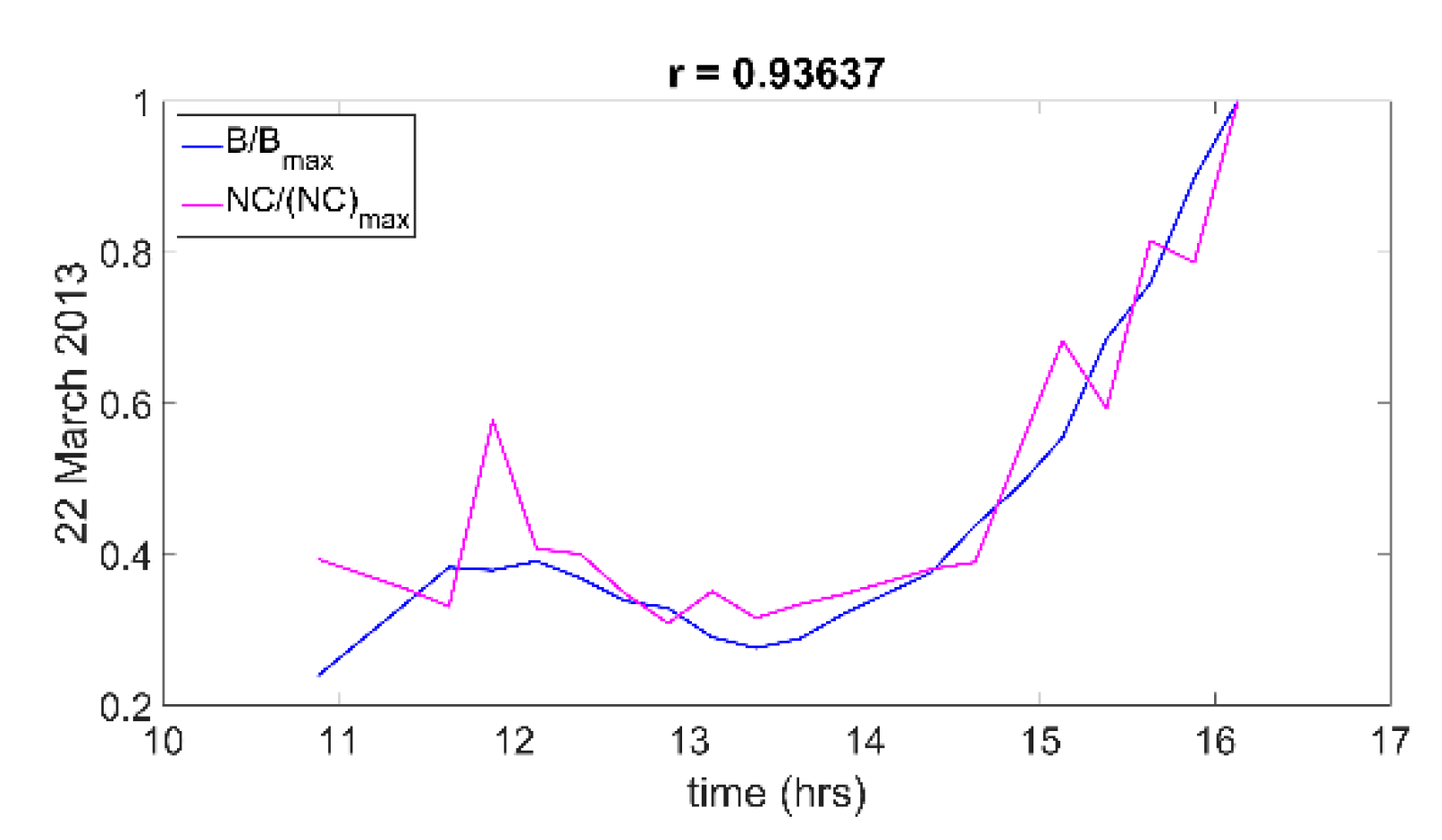
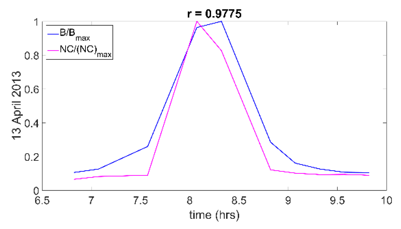
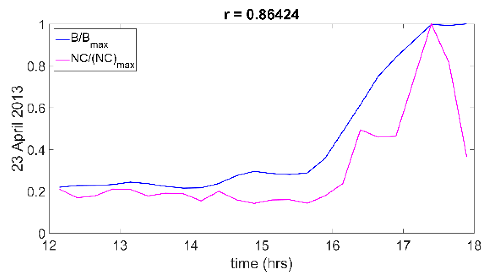
Figure 1. (Left) Scanning electron microscopy image of particulate aerosols, which are among the most common on the region, particle size can range from nanometers to microns. (Right) Panoramic photograph on a high-polluted day at El Paso-Juárez region, one can observe a clear a dusty cloud suspended at the atmosphere (Image credit: https://www.quora.com/ [What is the air pollution like in El Paso, TX?]).
Atmosphere 11 00866 g001
Figure 2. (ac) correspond to particle size distribution throughout the day on the selected representative days used to perform the inter-comparisons between the model’s scattering coefficients and the photoacoustic extinctiometer (PAX)’s corresponding results; (d) number of particles per unit volume and radii intervals (bins). From each graph, it is possible to observe and deduce a higher concentration of smaller size particles.
Atmosphere 11 00866 g002
Figure 3. Hourly inter-comparisons of scattering coefficients under low relative humidity (RH < 20%) using the models’ NC/(NC)max and the instrumentation’s results (B/Bmax) for 22 March 2013.
Atmosphere 11 00866 g003
Figure 4. Hourly inter-comparisons of scattering coefficients under low relative humidity (RH < 20%) using the models’ NC/(NC)max and the instrumentation’s results (B/Bmax) for 13 April 2013.
Atmosphere 11 00866 g004
Figure 5. Hourly inter-comparisons of scattering coefficients under low relative humidity (RH < 20%) using the models’ NC/(NC)max and the instrumentation’s results (B/Bmax) for 23 April 2013.
Atmosphere 11 00866 g005
Figure 6. Backtrajectories for 22 March 2013.
Atmosphere 11 00866 g006
Figure 7. Backtrajectories for 13 April 2013.
Atmosphere 11 00866 g007
Figure 8. Backtrajectories for 23 April 2013.
Atmosphere 11 00866 g008
Table 1. The second bin ( 0.25   μ m < r < 0.5   μ m ) is taken to be a mixture of soot and mineral dust. The given percentages on this table lead to the highest Pearson correlation coefficient, as represented on the last row.
22 March 201313 April 201323 April 2013
Soot57%11%25%
Mineral Dust43%89%75%
r0.966370.97750.86424

