Article

Refinements to Data Acquired by 2-Dimensional Video Disdrometers

by
Michael L. Larsen
1,2,* and
Christopher K. Blouin
1
1
Department of Physics and Astronomy, College of Charleston, Charleston, SC 29424, USA
2
Department of Physics and Atmospheric Sciences Program, Michigan Technological University, Houghton, MI 49930, USA
*
Author to whom correspondence should be addressed.
Atmosphere 2020, 11(8), 855; https://doi.org/10.3390/atmos11080855
Submission received: 12 July 2020 / Revised: 2 August 2020 / Accepted: 11 August 2020 / Published: 13 August 2020

Abstract

:
The 2-Dimensional Video Disdrometer (2DVD) is a commonly used tool for exploring rain microphysics and for validating remotely sensed rain retrievals. Recent work has revealed a persistent anomaly in 2DVD data. Early investigations of this anomaly concluded that the resulting errors in rain measurement were modest, but the methods used to flag anomalous data were not optimized, and related considerations associated with the sample sensing area were not fully investigated. Here, we (i) refine the anomaly-detecting algorithm for increased sensitivity and reliability and (ii) develop a related algorithm for refining the estimate of sample sensing area for all detected drops, including those not directly impacted by the anomaly. Using these algorithms, we explore the corrected data to measure any resulting changes to estimates of bulk rainfall statistics from two separate 2DVDs deployed in South Carolina combining for approximately 10 total years of instrumental uptime. Analysis of this data set consisting of over 200 million drops shows that the error induced in estimated total rain accumulations using the manufacturer-reported area is larger than the error due to considerations related to the anomaly. The algorithms presented here imply that approximately 4.2% of detected drops are spurious and the mean reported effective sample area for drops believed to be correctly detected is overestimated by ~8.5%. Simultaneously accounting for all of these effects suggests that the total accumulated rainfall in the data record is approximately 1.1% larger than the raw data record suggests.

1. Introduction

Disdrometers (from DIStribution of DROps METERS) are tremendously useful tools for precipitation science. Specifically designed to facilitate individual drop detection and measurement, disdrometers allow for determination not only of total integrated rain accumulations, but also for spatially and temporally localized estimates of the raindrop size distribution and related quantities like instantaneous rainfall rate R, radar reflectivity factor Z, rain kinetic energy flux density, and path-integrated attenuation [1]. As disdrometers measure a wide variety of relevant variables, they are frequently used in ground-truth studies to validate remote rainfall retrievals (see, e.g., in [2,3,4,5,6,7]).
There are many different disdrometers on the market, using a variety of measurement principles to reveal drop information (see, e.g., in [8]). One of the more sophisticated disdrometers available is the 2-Dimensional Video Disdrometer (hereafter 2DVD) manufactured by Joanneum Research in Graz, Austria [9,10]. This instrument now has a long history (the first prototypes were developed in the 1990s) and 2DVDs are extensively used in rain studies (see in [2,3,4,5,6,7,11,12,13,14,15,16,17,18,19,20,21,22,23,24,25,26,27,28,29,30,31,32,33,34,35,36,37,38,39,40,41,42,43,44,45,46,47,48,49,50,51,52,53,54,55,56,57] for a list of many of the works that have used this instrument for ground validation and/or rain microphysics studies).
The 2DVD has the capability of measuring several properties of individual hydrometeors falling through a sensing region of approximately 100 cm 2 . From these measurements, the associated software generates a record for each drop that includes precise detection time, estimated equivalent-volume diameter, fall velocity, oblateness, detection location within the sensing area, and an estimate of the effective detector area associated with the drop in question.
The reporting of a different effective detector area for each drop is an important feature of the 2DVD not often replicated in other disdrometer data records (though formulas to account for drop-diameter-dependent sensing area have been developed for other instruments, see, e.g., in [58,59]). The varying effective area in the 2DVD drop record is due to the requirement that any detected drop has to be fully within the field of view of both of the instrument’s line scan cameras. Consequently, the field of view for larger hydrometeors is smaller than the field of view for smaller hydrometeors. For example, a small 0.5 mm diameter spherical raindrop can still be detected even when its center lies 0.9 mm from the edge of a camera’s field of view. A 2.4 mm diameter spherical drop falling with its center the same 0.9 mm from the edge of the camera view is not recorded as part of the drop falls outside of the camera’s measurement domain and therefore the size of the drop cannot be reliably determined.
To account for this drop size-dependent sample area, the software supplied by the manufacturer adopts a drop-by-drop correction method similar to that suggested for other optical detectors; the default algorithm subtracts a drop diameter wide swath from the field of view along both cameras to determine the effective sensing area for each drop.
A proper computation of the effective sensing area can be more complicated than this. For example, it was recently reported [42] that all examined 2DVD data contains an intermittent anomaly. The anomaly directly affects a relatively small fraction of the total detected drops in most samples, but an estimated 15.5% of all drops (from a sample size of nearly 100 million detected drops) were detected during time intervals when part of the field of view gave spurious information [42]. Though the majority of the drops during this time are expected to be accurately sized, the effective sensing area should be decreased during those times to deduct for the part of the field of view that was giving unreliable information during drop detection.
Further complicating the story is the unfortunate fact that not all pixels in the 2DVD field of view correspond to equal areas. Because the field of view of the camera widens through the depth-of-field of the instrument, we find that the pixel size of the largest pixel in the field of view of the sensor has an area ~28% larger than the smallest pixel in the field of view. This has some (modest) impact to estimating the effective area for each detected hydrometeor not currently accounted for within the provided software.
In this work, we carefully revisit the algorithm previously described to flag spurious drops recorded during times of the intermittent anomaly [42]. An improved algorithm is presented that more accurately flags the spurious drops and identifies parts of the 2DVD field of view that are impacted due to the presence of the anomaly.
The second part of this study is devoted to properly assigning an effective sample area for each drop in a 2DVD data record. We explicitly correct the reported measurement area during times when the instrument is giving some anomalous data and correct for the varying pixel size throughout the 2DVD sensing region. The resulting algorithm finds alterations to the reported sensing areas for all drops, not just those measured during the anomalous time intervals.
After developing the algorithms to flag spurious drops and correct the effective sample area—a dataset acquired from two separate 2DVDs deployed near Hollywood, South Carolina is explored. This data record—comprised of approximately 200 million drops gathered over 667 daily observational data files—allows us to estimate the quantitative impact of the effects identified by the data processing algorithms presented here.

2. Materials and Methods

2.1. The 2-Dimensional Video Disdrometer

The 2-Dimensional Video Disdrometer (2DVD) made by Joanneum Research has been thoroughly described in the literature (see, e.g., in [9,10,60,61]), and its wide use suggests that the hydrological science community is well aware of the instrument’s relative strengths and weaknesses especially compared to other common drop detecting instruments like the OTT Parsivel and Parsivel2 detectors (e.g., [19,21,47,62]), Thies Clima Laser Precipitation monitors (e.g., [62,63]), Distromet Joss-Waldvogel impact disdrometers (e.g., [13,21,64,65]), and the Metek Micro Rain Radar (e.g., [29,47,65,66,67]).
Briefly, the 2DVD is comprised of two orthogonally aligned (but slightly vertically offset) high speed line scan cameras continuously recording images and detecting hydrometeors as shadows against an illuminated background. The projection of the camera sensing regions onto a plane has an intersecting region that defines the measurement area—a cartoon of a top-down view of the measurement geometry is shown in the left panel of Figure 1.
A 2DVD records drop detection time, volume, equivalent-volume diameter, fall velocity, and oblateness based on measurements related to drop residence time within the field of view of each camera, delay time between detection in the two vertically offset light sheets, and horizontal extent as estimated by the two mutually orthogonal horizontal line scan cameras. Moreover, reported are the pixels covered during maximal shadows along each camera’s field of view which allows for the approximate particle center location and footprint within the field of view to be reconstructed from the data record.
Spurious drop detection is minimized by the software’s “matching” algorithm that requires a candidate hydrometeor to be observed within the field of view of both line scan cameras with a plausible temporal separation. Potential “hydrometeors” seen only in one camera are not retained in the data record. This matching algorithm and the physical design of the instrument is specifically engineered to remove many of the spurious drops that are generated due to droplet impact with the physical structure housing the 2DVD [24], as well as insects and dust/debris.
The data analyzed in this study comes from two 2DVDs (SN074 and SN098) deployed at the College of Charleston at Stono Preserve near Hollywood, South Carolina. SN074 was installed in November 2013 at coordinates 32 44 26.2 N, 80 10 35.9 W, and SN098 was installed in May 2017 at coordinates 32 44 32.4 N, 80 10 29.6 W (approximately 250 m NE of SN074). Both sensors have had some downtime due to power outages, broken controller laptops, burnt out illumination sources, and internal clock generator outages, but both devices have been running the majority of the time as they were installed. The regular recommended maintenance has been performed to periodically recalibrate/measure the vertical distance between the horizontal light sheets and recalibrate the internal sizing algorithm. The instruments have been validated against each other and against measurements taken with an array of Thies Clima Laser Precipitation Monitors [24,30,33,42,68]. Additionally, a previous study took an in-depth look at the data from these sensors and four other 2DVDs and did not reveal any notable discrepancies in the general structure of the data [42].

2.2. The Data Anomaly

Despite the fact that the instrument was specifically designed to minimize false detection of non-hydrometeor particulates, it has recently been revealed that 2DVD data has persistent anomalies that are detectable in all examined 2DVD data records [42].
The physical origin of the anomaly is clear. During a rain event, a persistent obstacle (possibly a fragment of a natural raindrop) covers a portion of some of the internal optics of the detector associated with one of the line scan cameras. The obstacle generally only persists for a brief period of time but, while present, the obstacle creates a signal in the associated line scan camera consistent with the constant detection of a potential hydrometeor. This alone is not enough to induce a false raindrop detection, but if paired with a real hydrometeor (or an insect, drop fragment, dust, etc.) that is outside the desired sample area but still detectable by the other line scan camera, it can cause a droplet to be artificially added to the data record with physically meaningless properties. Even if this detected drop is real but outside the field of view, the reported diameter, position, and fall speed will not be accurate.
The persistent obstacle can stay on the optics for time intervals varying from a small fraction of a second to a sizable fraction of an hour, with the median anomaly duration estimated at about half a second [42]. Normally this optical obstruction will induce false detections of drops along a line of pixels within the field of view.
Also possible (but more rare) is if the anomaly is present in the hourly instrumental recalibration of the 2DVD’s video level renormalization; when this occurs it artificially lowers the baseline video intensity level to the point where no subsequent drops can be successfully detected along a line of pixels within the field of view until the next renormalization. This is a way in which the anomaly can temporarily prevent the detection of drops within part of the measurement area of the sensor.
Because drop arrivals are stochastic events that can naturally occur in bunches and clusters ([69,70]), drop detection times alone do not help to identify artificial drops in the data record. Fortunately, a “heat map” of the detected arrival positions within the sensing area can be used to clearly identify when an anomaly was present. In [42], an algorithm was developed that uses temporally localized drop detection spatial statistics to infer whether an anomaly was present and to flag suspect drops. Subsequent analysis presented in that work revealed that this anomaly appears in all 2DVD data available and 1–5% of drops detected are likely completely spurious due to this anomaly. These spurious drops can occur during high or low rain rates, may be sized as large or small diameter drops, and are not notably more or less likely to deviate from the expected vertical fall velocity.
As the spurious drops can be identified by the flagging algorithm developed in [42], one might hope that a dataset can be corrected by merely removing the non-real drops from the data record. Unfortunately, some real drops are not accurately measured during this time in the part of the sensing area where the anomaly occurs. A full correction should adjust the effective sample area accordingly. To make this adjustment, the flagging algorithm presented in [42] needs to be improved.
The algorithm as presented in [42] used the particle midpoint along each camera’s field of view to specify a location of the particle center (in half-pixel resolution) for each drop. Based on a histogram of the 1000 most recent drop arrivals into 10 pixel wide regions, histograms along both camera fields of view could be sequentially examined to see if any particular line of pixels were anomalously “hot” with extra droplet detections or “cold” with too few droplet detections. If such pixel regions were identified, all 1000 detected hydrometeors in the “batch” were flagged and an additional flag was created for those hydrometeors that were in the anomalous time interval AND had their centers in a “hot” region.
Although this flagging algorithm was able to crudely establish the relative prevalence of the anomaly, the code utilized some non-optimal arbitrary parameters (e.g., the use of 10 pixel domains, the use of the 1000 droplet “batch size”, and the thresholds for when droplet counts were sufficiently high or low to trigger the “hot” or “cold” condition, respectively). Subsequent analysis reveals that a more robust algorithm can be applied; although still not devoid of all arbitrary parameters, the new algorithm improves the previous flagging code in the following ways.
  • Rather than grouping into 10 pixel domains, the new algorithm looks at each pixel along both camera fields of view.
  • Rather than assigning a droplet position to be at its detected center, the new algorithm looks at every pixel covered by every recorded hydrometeor in the “batch”.
  • The old algorithm used the ith through the (i + 1000)th particle detection to determine whether the ith particle was anomalous; the new algorithm uses the (i − 500th) through (i + 500th) particle detection, helping to localize anomalies more accurately in time.
  • The old algorithm had no way of handling the last 1000 drops in a dataset; the new algorithm modifies the algorithm slightly for the first 500 and last 500 drops of a sample; although anomaly detection is arguably not ideal for these drops, it is possible to flag drops throughout an entire day’s accumulation so long as it lasts at least 1000 drops.
  • Anomalies resulting in underdetection due to an obstacle on the optics during the hourly renormalization of video levels typically have long duration and involve a more subtle detection than the spurious drop-creating anomalies. Because of this, a larger window of 10,000 drops are used for detection and confirmation of the under-detection phenomena. A similar adjustment to centering the window on the drop in question (instead of just looking at the following 10,000 drops) is also applied to the underdetection algorithm.
This new “deglitch code” was compared against the version introduced in [42]. By comparing flagged drops to those visually identified by looking at heat-maps of drop arrivals, it is clear that the new algorithm is doing a more reliable job of identifying spurious drops and isolating times of increased and decreased instrumental sensitivity in part of the cameras’ joint field-of-view. Using the new algorithm, the basic qualitative results in [42] seem to hold, but more complete and accurate information is obtained that allows for a modified estimated sample area calculation.
More details regarding the logic for this improved algorithm are presented in Appendix A.

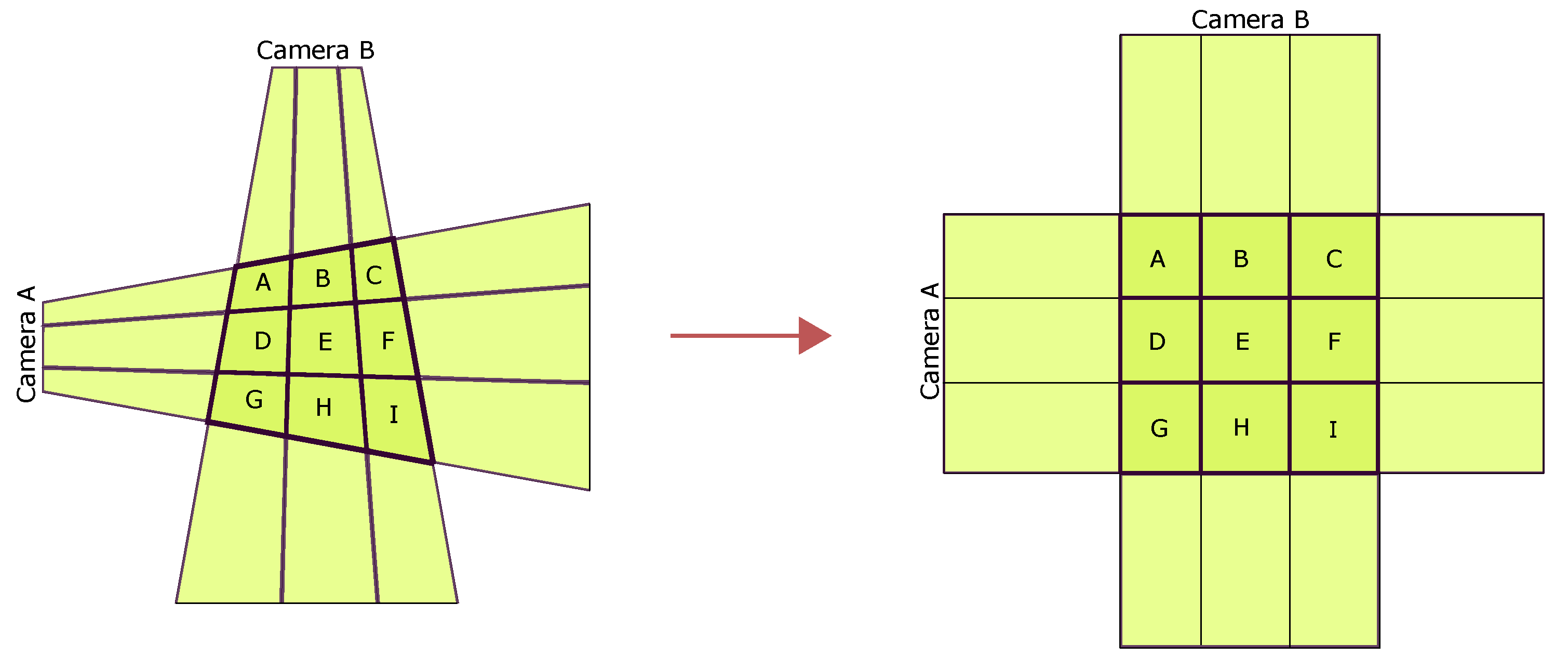
2.3. Calculation of the Effective Area

As noted in [9], the drop size distribution N ( D ) can be estimated from 2DVD measurements via
N ( D i ) = 1 Δ t Δ D j = 1 M 1 A j v j
where N ( D i ) is typically measured in m 3 mm 1 , Δ D is the width of the diameter bin (in mm; typically taken to be 0.2 mm for 2DVD data due to a nominal pixel resolution of about 0.17 mm), Δ t is a time interval associated with the DSD estimation interval (often 60 or 300 s), v j is the measured drop fall speed of the drop in m s 1 , A j the effective instrument sample area in m 2 , and M the number of observed drops in the specified diameter class during the specified time interval.
The rain rate R (typically measured in mm h 1 ) can be computed either by starting with the drop size distribution above, or alternatively directly from the (binned or unbinned) drop record via:
R = 1 Δ T i = 1 N π 6 D i 3 a i
with Δ T again the time interval associated with the rain rate temporal estimation interval (this time using T instead of t to emphasize that in this formula the time is expected to be in units of hours), D i the (binned or unbinned) spherical-equivalent diameter of the ith detected drop in the time interval (in mm), a i the effective instrument sample area for the ith drop (this time in mm 2 ), and N being the total number of detected drops in the associated time interval. The formula most frequently used for rain rate in the literature gives the same quantitative value but determines this quantity from N ( D ) and thus includes prefactors for converting between seconds to hours and m 2 to mm 2 (see, e.g., in [22,27,37]). As rain rate is fundamentally a quantity related to a surface flux (total depth accumulated over a surface), deriving the rain rate estimation through the volume-based raindrop size distribution seems less direct, and consequently we will use Equation (2) (see a more complete discussion in [71]).
A key observation is that both N ( D ) and R rely on a drop-by-drop estimation of the effective sample area of the detector. For some disdrometers (e.g., the Joss–Waldvogel impact disdrometer), this detector area can be treated as a constant with minimal error and factored out of the associated sum. In the case of the 2DVD, we are aware that the effective sample area depends on the size of the drop. It is because of this that the effective sample area is one of the output fields of the drop record in 2DVD data.

2.3.1. Computation of the Effective Area by the Included Software

There are slight differences between the optical alignments in different 2DVDs, and because of this the effective pixel size in the middle of the sample area of each 2DVD can be slightly different. The documentation supplied when purchasing a 2DVD reports this value, for example, the calibration sheets for 2DVD SN074 report this value as 0.167 mm/pixel and the value for SN098 has values of 0.165 mm/pixel and 0.164 mm/pixel for cameras A and B, respectively. Thus, even if the drop diameter-dependent excluded area near the edge of the field of view was completely unaccounted for, the reported area for identical drops falling through the two detectors would be slightly different. This is borne out from the data archive. The approximately 146 million drops examined from SN074 has an average reported area approximately 3.2% larger than the average reported area from the approximately 56 million drops examined from SN098. As ( 0.167 mm ) 2 / [ ( 0.165 mm ) ( 0.164 mm ) ] 1.031 , this is almost exactly what should be expected.
By utilizing the area measurements reported by the 2DVD software, we were able to recreate the internal manufacturer algorithm for droplet effective sample area. First, take the number of pixels in the total field of view for each camera (632) and subtract (2 + D pix ), where D pix is the estimated diameter of the drop (in pixels, rounded up to the nearest integer). Then, calculate the area as ( lpp A ) ( lpp B ) ( 630 D pix ) 2 , where lpp A and lpp B are the lengths per pixel values for cameras A and B in the instrument documentation.
The reason for the subtraction of 2 pixels in addition to the estimated drop diameter is presumably because there must be at least one non-occluded pixel at the edge of the measurement area to successfully detect and size a particle. Thus, on each side of each camera’s field of view there must be at least ( 1 + ( D / 2 ) pix ) pixels between the edge of the camera’s view and the midpoint of the detected hydrometeor.
We believe there are several issues with this formulation:
1
All pixels within the field of view are treated as having the same area.
2
The edges of the sample area are not accounted for perfectly and, although an exact correction is not possible for pixelated data, an improvement can be made.
3
Reductions in effective measurement area during the previously described anomaly are not provided.
Each of these issues are addressed in the following sections.

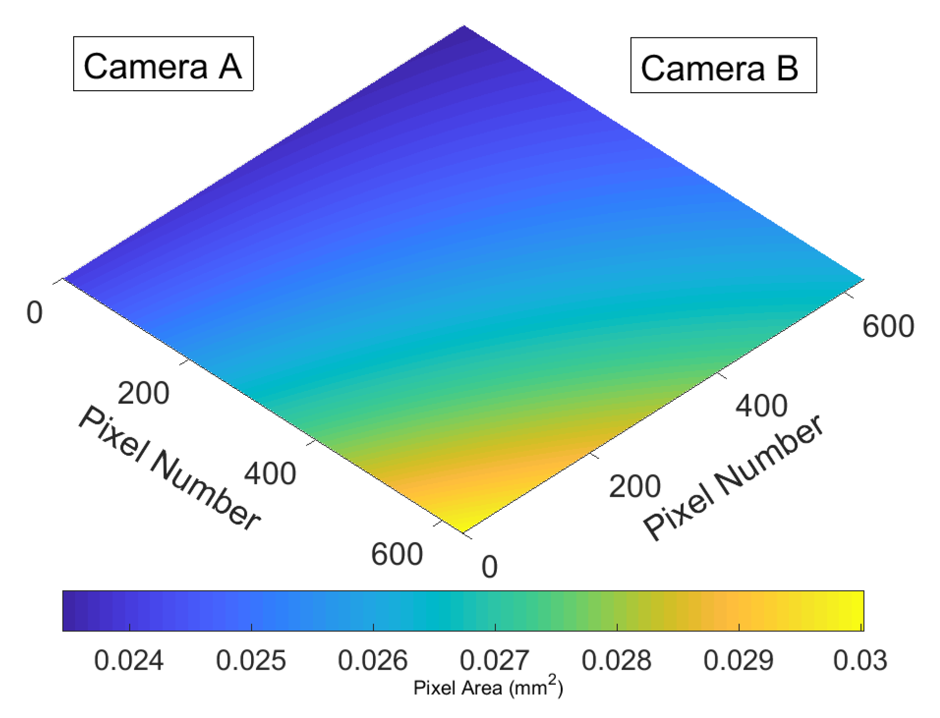
2.3.2. Areas of 2DVD Pixels

As suggested by the cartoon in Figure 1, not every pixel has the same area. Though the sensing area is often drawn as the intersection of two rectangles, resulting in square pixels as in the right panel of Figure 1 (see, e.g., in [9,42]), a more accurate depiction is that the reconstructed sample area is the intersection of two trapezoids. This means that each pixel is appropriately described as an irregular quadrilateral.
Measurements of the detailed 2DVD optical geometry were made by manually placing digital calipers in the field of view of each camera at several places along the optical path. A schematic indicating the locations that the optical distances were measured is shown in Figure 2.
After the light from the illumination source passes through the Fresnel lenses, there are no optical elements between the light source and the camera except for a single flat mirror. Because of this, the illumination throughout the interior of the instrument can be reliably described as a light sheet that narrows as it approaches the camera.
Multiple measurements of all the dimensions shown in Figure 2 were made with a calipers (except for F and M which were measured with a meterstick since these distances were larger than the calipers available). The mean results for the measurements for both 2DVDs are shown in Table 1.
Based on the detailed camera geometry, an estimation of how the pixel dimensions change with position within the sensing area for each detector was obtained. A detailed description of this computation is presented in Appendix B, and we have generated a code that will allow other investigators to determine the area of each pixel of other 2DVD instruments if the measurements illustrated in Figure 2 can be taken.
As can be seen from Figure 3, the differences between pixel areas in different parts of the field of view can be non-negligible; the pixel with the largest area within the sample area is ~28% larger than the pixel with the smallest area. Results for 2DVD SN098 are similar—again with an ~28% difference between the largest and smallest pixels—though corresponding pixels are a few percent smaller in SN098 (consistent with the manufacturer’s documentation that indicates that the field of view in SN098 is a little smaller than for SN074).
Despite a difference of ~28% in pixel area on the extremes of the measurement volume, the non-constant pixel areas do not typically drastically alter the total effective area estimation given by the manufacturer as the included software’s algorithm described previously removes pixels around the entire outer boundary, thus removing as many smaller-than-average pixels as larger-than-average pixels when computing the area. The real importance of identifying the area associated with each pixel comes when (asymmetric) portions of the central sensing area must be deducted from the effective sampling area due to the presence of the anomaly described earlier; in these cases assuming every pixel has the exact same area can cause larger errors.

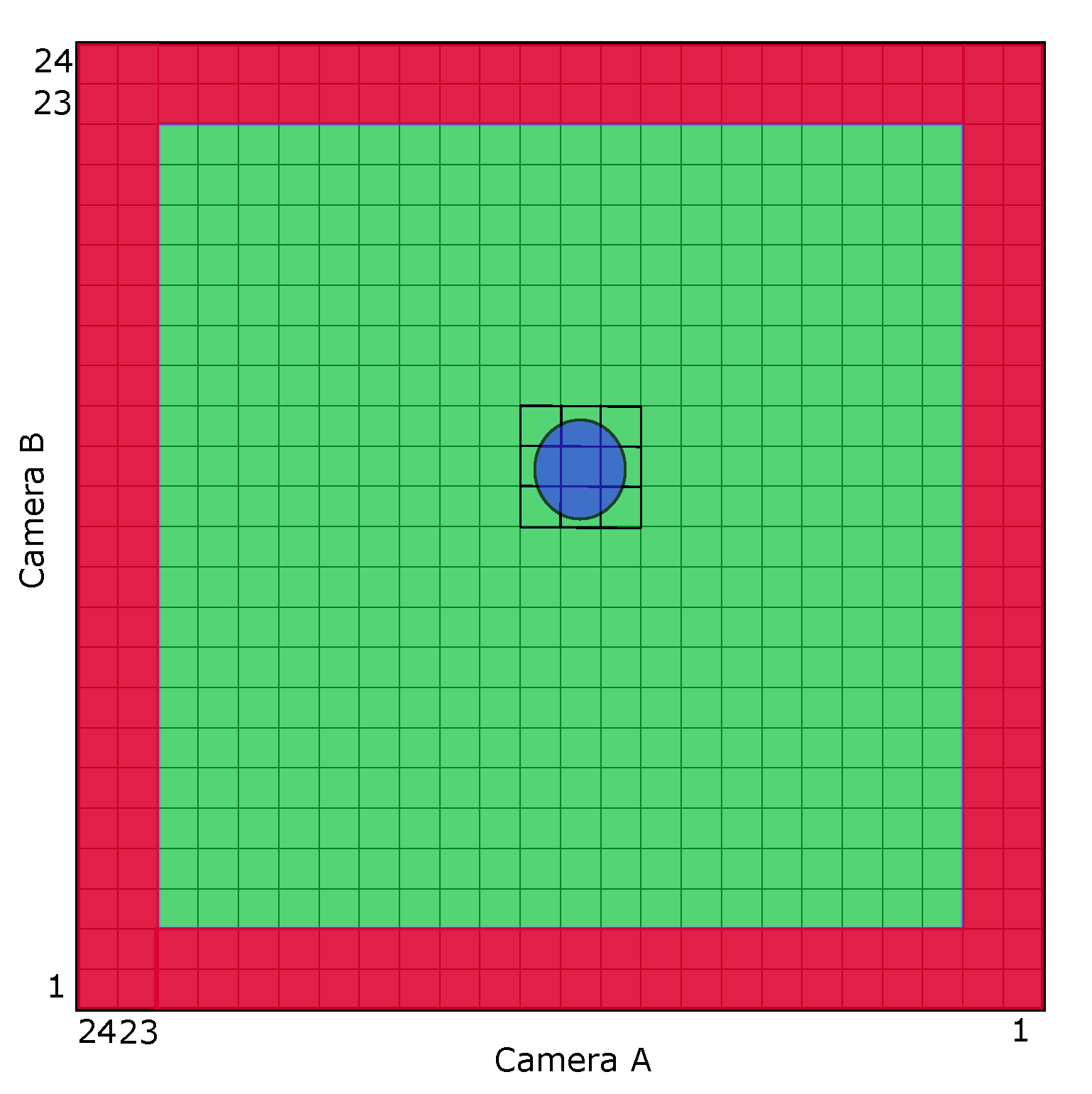
2.3.3. Accounting for the Boundary

Properly accounting for how many pixels to remove from the effective area as a function of drop diameter is complicated. The manufacturer algorithm is a good approximation, but improvements can be made.
Consider the cartoon in Figure 4 that (for simplicity) represents the sample area as a square with a regular grid. For simplicity, the grid is drawn with only 24 pixels on a side, and we consider a drop with diameter and alignment relative to the underlying grid that covers a 3 × 3 domain and thus would be reported to have a diameter corresponding to 3 pixels. Because this droplet occludes an odd number of pixels in each camera, its center could be anywhere within the green region and still be detected with at least one half pixel remaining uncovered at the boundary. (Only 51% of a pixel needs to remain uncovered for the internal logic of the 2DVD to treat a pixel as non-shadowed [9]). Thus, a proper treatment of this drop would retain all of the green pixels—removing 2 pixels from the edge all around the sample area when computing the effective area of the sensor for the drop in question.
Another common, but more complicated, scenario is shown in the left panel of Figure 5. Here, the drop is exactly the same size as shown in Figure 4 but aligned with respect to the underlying tesselation created by the cameras such that only 2 pixels are occluded along the vertical direction, whereas 3 pixels are still occluded along the horizontal direction. In a scenario like this, the particle center could be in the “inside-half” of the blue shaded regions and still occlude less than half of the boundary pixel. To account for this sort of drop properly, the algorithm we have developed includes half of the area associated with pixels colored blue and all of the area from pixels colored green. Note the interesting consequence that identical drops could potentially have different measured diameters and different effective sample areas depending on how the drop’s fall position aligns with the underlying camera grid.
The right panel of Figure 5 shows the same hypothetical drop now aligned relative to the background grid so that only 2 pixels are occluded along the field of view of both cameras. As was seen in the left panel, the droplet center could have fallen anywhere in the “inner half” of the blue pixels and still had a pixel illuminated and unblocked by the drop on the boundary allowing for proper detection. The orange pixels only allow for detection with an undetected border pixel in both cameras if the drop center lies in the innermost quadrant of the pixel, so only 1/4 of the area of those pixels are included in the new algorithm’s sample area calculation.
The general rules demonstrated in Figure 4 and Figure 5 are extendable to other detected drop sizes and the full 632 pixel wide field of view of both cameras; a border that depends on the drop’s detected horizontal dimensions can be applied to the default sample area.
The results from the area calculation described here are slightly different than those applied by the manufacturer’s software because (i) the algorithm we develop identifies the parts of the image domain where pixels are removed and uses the areas of those particular pixels, and (ii) the number of pixels removed around the boundary is not always exactly the same as in the supplied software.
To be more explicit, consider the scenario shown in the left panel of Figure 5. As the picture reveals, a total of 4 pixels (1, 2, 23, and 24) are removed from Camera A’s view whereas a total of 3 pixels (1, half of 2, half of 23, and 24) are removed from Camera B’s view. The manufacturer-supplied algorithm looking at the same drop would remove a total of either 4 or 5 pixels (depending on whether the assigned diameter ends up closer to 2 or 3 pixels, which partially depends on the 2DVD’s measurement of the height of the droplet) from each camera’s field of view. The manufacturer-supplied algorithm also treats every pixel as having the exact same size when computing the remaining effective sample area.
The difference between the manufacturer’s algorithm and the method described above is admittedly small, but these slight corrections can be applied to every drop detected in every 2DVD record.

2.3.4. Removal of Insensitive Part of the Field of View during the Anomaly

Although correcting for nonuniform pixel areas and slightly modifying the treatment of the boundary should modestly increase the accuracy of the effective area, the primary reason for revisiting the effective area calculation is to correct the effective sample area for the properly detected drops measured during the times of partial instrumental insensitivity due to the anomaly described in Section 2.2 and in [42]. Figure 6 shows a cartoon of the area-adjustment algorithm developed for this case.
An anomaly—whether it is of the type that causes spurious drop detections or of the type that induces insensitive regions within the field of view—renders the associated part of the sample area ineligible to contribute to drop detection. In addition, a guard area (not unlike those already computed at the camera boundaries) must be applied to the part of the field of view adjacent to the anomalous region; any drop falling close enough to the regions marked in black would not have their size reliably recorded and may be missed entirely.
Because of this, the improved flagging algorithm identifies and flags drops with any portion of the drop sufficiently close to the unreliable regions (marked in black in Figure 6). Additionally, all drops that have the flag indicating “detected during a time interval when an anomaly was present” have a drop size-dependent subset of the detector sample area removed from its reported effective sample area. Referring back to Figure 6, a drop with the recorded dimensions of 3 pixels in the camera A axis and 2 pixels in the camera B axis could only have fallen in the green pixels and half of each blue pixel while being successfully recorded and accurately sized. A drop falling with its center in the interior red or blue regions may have been recorded, but the developed algorithm assigns a flag indicating the drop detection may not be reliable as the size or fall velocity of such a drop may have been artificially inflated or diminished due to the static obstacle in the camera image. Removal of all of the black and red pixel areas and half of the blue pixel areas can noticeably reduce the effective sample areas for all drops during the times of the instrumental anomaly–even for drops that are not near the problem region of the detection area.

2.3.5. Mean Pixel Size

By far the largest change from the manufacturer-reported sample area is due to the simplest effect; in both SN074 and SN098 our measurements support a mean pixel sample area slightly smaller than that reported by the manufacturer.
As noted above, the manufacturer-reported pixel area is assumed uniform throughout the effective area algorithm; for the 2DVDs used in this study that area is taken to be ( 0.167 mm ) 2 0.0279 mm 2 for 2DVD SN074 and ( 0.165 mm ) ( 0.164 mm ) 0.0271 mm 2 for 2DVD SN098.
The measurements presented in Table 1, however, suggest that these mean pixel areas should be 0.0258 mm 2 for 2DVD SN074 and 0.0254 mm 2 for 2DVD SN098. This change of approximately 7–8% of the reported value was large enough that we reverified the optical dimensions of the sensing area multiple times. We estimate our measurement uncertainty at 1 mm based on the variability between independent measurements and the precision of the calipers used. Even a hypothetical 1 mm systematic error in all measurements would only account for about half of the difference between our estimated value and the fixed value used by the manufacturer’s algorithm.
This is particularly notable since it suggests that all rain rates derived from 2DVD measurements that utilize the manufacturer-supplied effective area field may be in error by approximately 7–8% before accounting for other measurement uncertainties like particle sizing or spurious drop detections.

2.3.6. The New Effective Area Algorithm

The phenomena described above led us to develop a new algorithm that can recompute the effective sample area for each drop based on 2DVD output in conjunction with a pixel-area lookup table that can be generated by taking measurements of the labeled dimensions on Figure 2. The algorithm is not currently well optimized (processing 10 years of archived 2DVD data takes five high-end machines the better part of a week), but a working version can be made available to other investigators who wish to apply it to their archival 2DVD data. Here, we describe the underlying logic of the algorithm.
First, the relevant optical dimensions of the field of view of a 2DVD as shown in Figure 2 are carefully measured. From this, the coordinates of each pixel’s vertices are determined and the area of every quadrilateral is computed and stored in a look-up table; 2DVDs with different serial numbers will have different look-up tables.
Second, the recorded drops are examined. For each detected drop a weighting factor is defined for each pixel in the sample area. Based on the detected dimensions of the drop along each camera axis and the drop’s detected position, each pixel is assigned a “weighting factor” of 1, 0.5, 0.25, or 0. The weighting factor of 1 is chosen if the drop falling anywhere in the pixel in question could have been reliably sized and detected, like the green pixels in Figure 4, Figure 5 and Figure 6. Similarly, the other weighting factors are chosen if only half (depicted by blue pixels), a quarter (orange pixels), or none (red or black pixels) of the pixel could serve as the center of a properly sized and detected drop due to proximity to the boundary or an insensitive region of the detector.
Each pixel’s geometric area (computed in the first step) is then multiplied by the associated weighting factor (computed in the second step) for the drop in question, and the total weighted area for the entire field of view corresponds to the corrected effective sample area of the detector for the drop. More succinctly, the effective area of the ith drop can be computed from
a i = k = 1 632 2 w i k α k ,
where w i k is the weight of the kth pixel for drop i (which depends on the fall position and the dimensions of drop i) and α k is the area of the kth pixel (in mm 2 ).

3. Results

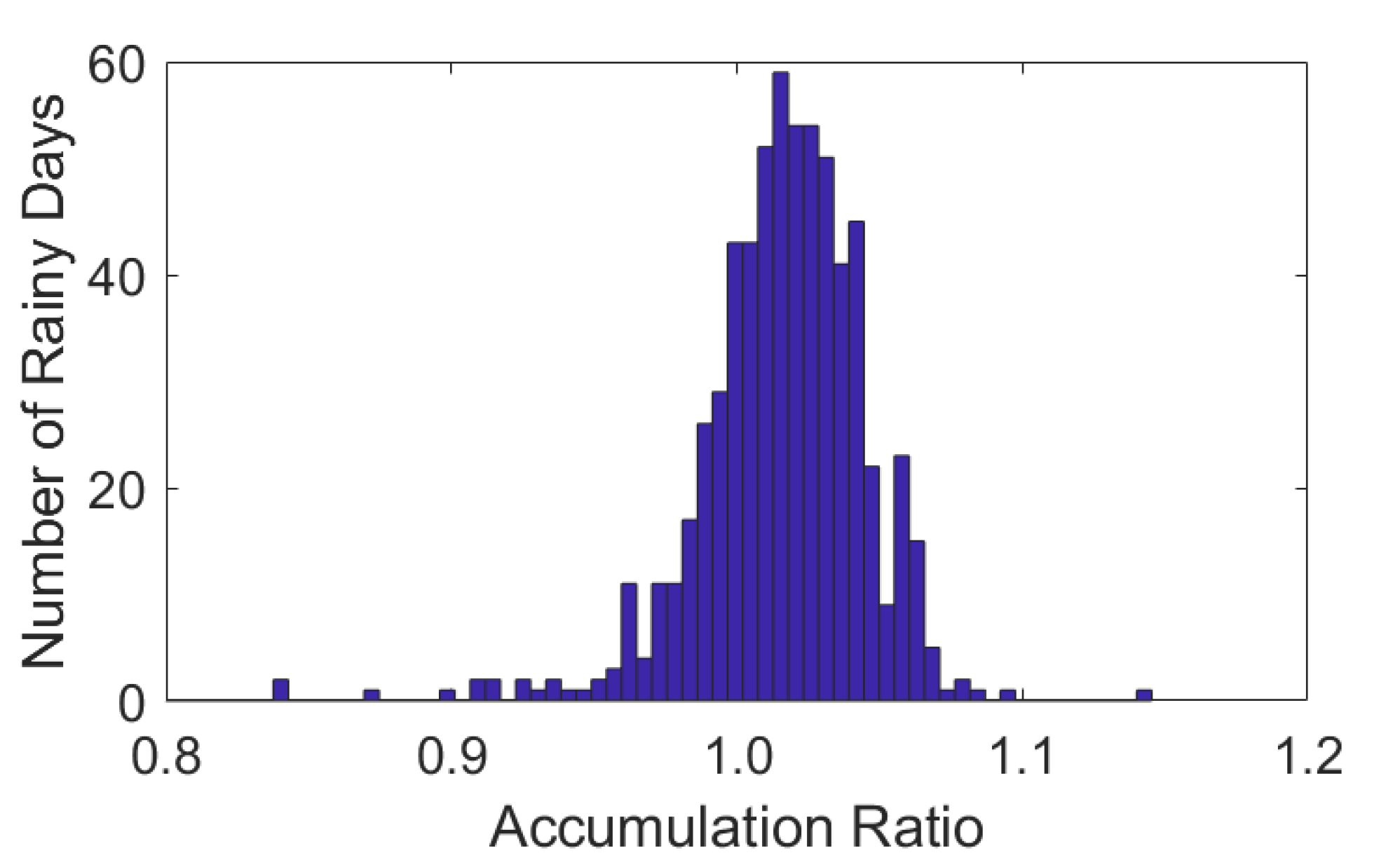
3.1. Ensemble Results
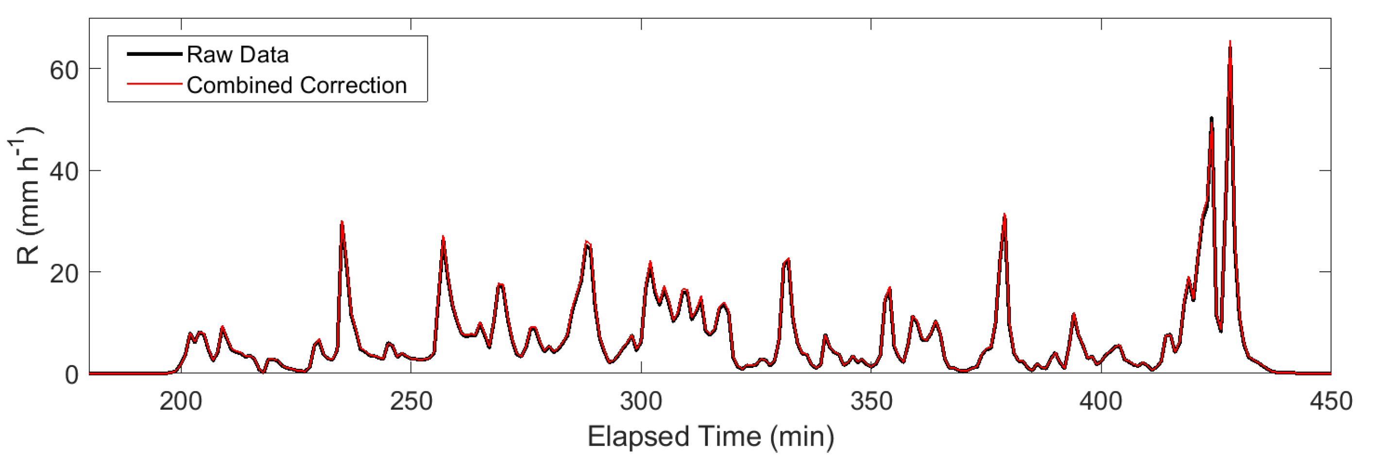
2DVD serial numbers 074 and 098 were installed at the College of Charleston at Stono Preserve in 2013 and 2017, respectively. For the sake of this analysis, the data from each instrument’s installation date through 10 May 2020 is utilized. For this time interval, SN074 provided data files for 1812 out of 2330 possible total dates (77.8%) and SN098 provided data files for 776 out of 1091 possible total dates (71.1%). As the anomaly flagging algorithm does not perform optimally for the first 5000 and the last 5000 drops in a day’s data (see Appendix A), we limited our analysis to daily records where at least 20,000 total (non-spurious) drops were detected to ensure that the majority of each day’s drops had optimal sensitivity to anomaly detection. This left a total of 667 days of data in the ensemble (491 days from SN074 and 176 days from SN098). This data record includes a total of 202,555,318 drops (194,089,999 when the spurious drops are removed) and an estimated total accumulation depth of 7124.3 mm (when using a i as computed in Equation (3) and removing the drops flagged as spurious).
Table 2 summarizes the bulk statistics under different analysis methods. In general, it appears that the ensemble statistics are very sensitive to the choice of whether (and how) to bin the drop diameters—an observation that has been made in other contexts before (see, e.g., in [72,73,74]). No matter which method is used to bin diameters, however, it appears that the net influence of all of the effects explored in this study are comparatively modest when examining the statistics related to the full ensemble; the difference between including removal of spurious drops while fixing the area and neglecting both effects is less than 1.2% for total accumulated depths and mean diameters.
The small net effect can be deceptive. Only removing the spurious drops (while not fixing the effective sample area) results in reduction of the estimated accumulation depth by approximately 7–8% (depending on the diameter binning paradigm used). Similarly, only adjusting the effective area while not removing the spurious drops results in enhancement of the estimated accumulation depth by approximately 12–13%. As these two factors are similar in magnitude and adjust the accumulated rainfall in opposite directions, the resulting net effect is very small. Looking at the ensemble-summed magnitude of each correction in isolation makes the net change hard to predict because time intervals having large numbers of spurious drops also require the largest area corrections for the drops that remain.

3.2. Event Analysis

Analysis of daily rain records in the ensemble reveals that the net impact from spurious drops and effective area adjustments does remain small. Figure 7 shows a histogram of the ratio between the modified daily accumulation and the uncorrected accumulations.
It appears that even though the magnitude of the area correction is larger than the correction due to spurious drops on average, the removal of spurious drops actually lowers the total estimated accumulation on approximately 1/4th of the daily data records. Approximately half of all of the daily records show an accumulation increase between 0% and 4%, and deviations from the uncorrected data record that exceed 10% in either direction occur less than 1% of the time.
Even though daily accumulations are not modified very much, it could still be possible that certain times within a daily data record could be more drastically impacted. To explore this, a single rain event from 18 February 2020 has been chosen for further study. This rain event was approximately 4 h long and was detected by both SN074 and SN098. Total estimated accumulations from the uncorrected raw data total 30.2 mm (SN074) and 29.5 mm (SN098). After removing spurious drops and using the area algorithm presented here this alters the estimated accumulations to 31.1 mm (SN074) and 29.6 mm (SN098).
A time series of the 1 min rain rate is presented for SN074 in Figure 8. Note that, even on 1 min timescales, any impact to rain rate is hard to identify.
The quantitative impact can be better observed by carefully looking at a subset of the same event. Figure 9 shows about a half-hour portion of the event with separate traces for the raw data, area correction only, spurious drop removal only, and the combined impact from both corrections. Similar to the results observed for the entire data ensemble, we see that the area correction and spurious drop removal modify the uncorrected data in opposite directions and combine for a small overall change in the estimated rain rate.
Another way to visualize the impact from applying the correction for this event’s data is to examine the ratio between the corrected rain rate and the uncorrected rain rate for each minute; this is shown in Figure 10. It appears that the ratio between the corrected and uncorrected R values are typically positive during times of low rain intensity and closer to unity at higher rain rates. This makes intuitive sense: at low rain rates it is expected to be less likely that a drop fragment would splatter and cover the 2DVD optics and therefore spurious drops are expected to be infrequent. The relative paucity of spurious drops at low R results in the area correction having a greater influence than the spurious drop correction during most small-R temporal intervals.
Although only results for SN074 are shown here, similar behavior is seen for SN098. It seems that the corrections due to the algorithms here are typically very small unless the data is cut down to very small subsets.

3.3. Individual Drops

In order to continue the trend of exploring increasingly smaller subdivisions of the data to reveal more pronounced effects, we extend our examination to the smallest possible scale—the scale of individual drop detections. Figure 11 shows a histogram of the effective sample area ratios for retained drops in the entire ∼200 million drop ensemble.
Perhaps most notably, our measurements suggest that there is a significant difference between the manufacturer-used mean pixel area and the measurement-supported mean pixel area. The ~3% difference between our measurements of the pixel width at the midplane and the value hard-coded into the processing algorithm accounts for most of the mean shift of approximately 8–9% seen in the figure.
The spikes in the histogram for area ratios between approximately 0.92 and 0.94 make sense; these cases correspond to scenarios like those shown in Figure 4 and Figure 5, where the differences between the manufacturer-reported area and the corrected area only have to do with the overall sample area estimation, slight changes due to the non-constant pixel sizes, and slight differences in how many pixels are removed from the boundary of the field of view. The broader feature centered at approximately 91.5% and extending from 87% to 93% shows the impacts of the anomaly; drops having this area ratio have a larger fraction of the field of view removed due to instrumental insensitivity (as was schematically shown in Figure 6.) The feature is broader than the spikes between 0.92 and 0.94 because the amount of area removed depends on the pixel dimensions in the part of the sample area temporarily insensitive to drop detection.

4. Discussion and Conclusions

The 2DVD is widely used in hydrological science and many of its features and deficiencies have been discussed at great length (see, e.g., in [9,10,60]). To date, however, a careful assessment of the reported effective sensing area has not appeared in the literature. In an effort to investigate questions related to drop detection area, it was necessary to substantially improve the previous algorithm to flag spurious drops improperly detected due to persistent optical obstacles. The improvements to the algorithm allow for better temporal localization of anomalous data and identify which part(s) of the sensor sampling area are inaccessible during the anomaly.
Examination of an ensemble consisting of over 2 × 10 8 drops collected over 667 observation days reveals that approximately 4.2% of all detected drops were spuriously recorded due to the anomaly described in [42]. Of the drops that remain after filtering out the anomalous drops, it was found that all reported effective sensor sample areas are overestimated by at least 6.5% with the median (mean) error overestimating areas by 8.3% (8.5%).
The total impact when correcting for both factors results in an increase in total accumulation estimates of ~1.1% for the ensemble. The effects largely compensate for each other since removal of spurious drops decreases the total rainfall accumulation and decreasing the effective area increases the computed rainfall rates through the denominator of Equation (2).
The resulting change of only ~1.1% may be surprising; this arises out of a subtle coupling between the two effects. A drop either is or is not spurious, and, although all droplets require a effective area adjustment, the largest adjustments occur during times of spurious drop detection when an interior portion of the 2DVD field of view needs to be removed from each detected droplet’s effective sensing area. As spurious drops tend to occur during high rain rates, the removal of spurious drops and large effective area adjustments are not decoupled independent events. Consequently the total impact on accumulation totals cannot be easily determined by merely multiplying the fraction of the remaining drops by the mean enhancement due to effective areas found by decreasing the denominator of each term in Equation (2).
Analysis of 667 one-day total accumulation estimates shows that full-day estimates can be modified by up to 15%, but most daily totals are modified by substantially less than this with half of the daily estimates increasing from 0% to 4% (see Figure 7).
The quantitative impact from the spurious drop and sensor area errors is presumed to be much smaller than other concerns about the 2DVD related to decreased sensitivity and accuracy in detecting small drops, influence of horizontal wind, and investigator choice of diameter binning methodology. However, it is nevertheless noteworthy that the effective area measurement influences the properties of every detected drop and impacts all estimates of bulk quantities like rain rate and drop size distribution; the effective sensing area for each drop appears in the formulas to compute these quantities (see Equations (1) and (2)). Because algorithms to correct for these errors are now available and the effects on 2DVD data affect all detected drops, we recommend the codes to flag/remove spurious drops and adjust estimated sensing area should be utilized when using 2DVD data for ground validation or instrument inter-comparison purposes.

Author Contributions

M.L.L. led contributions associated with conceptualization, data curation, formal analysis, funding acquisition, investigation, project administration, resources, supervision, and writing the original draft. M.L.L. also assisted in the associated software development and bug checking. C.K.B. led contributions associated with software development and bug checking. C.K.B. also assisted with formal analysis, investigation, and wrote parts of the original draft. Both authors were involved in the review and editing tasks of the writing process. All authors have read and agreed to the published version of the manuscript.

Funding

This research was funded by the National Science Foundation through grants numbered 1230240, 1532977, 1823334, and 2001490 (M.L.L.) and through the College of Charleston Summer Undergraduate Research with Faculty program (C.K.B.).

Acknowledgments

Thanks to Gavin Connors, Eric Davidson, Joerael Harris, Günter Lammer, Robert Lemasters, Monica Mullis, Joseph Niehuas, Michael Schönhuber, Martin Schwinzerl, and Joshua Teves for their help in keeping the College of Charleston 2DVD instruments operating over the life of the project. Thanks also to Trey Anderson and Bridget Ierace for independent verification of 2DVD area measurements. Finally, the authors thank the anonymous reviewers, who had insightful comments and suggestions for the first draft of this manuscript.

Conflicts of Interest

The authors declare no conflicts of interest.

Appendix A. Details Regarding the Improved Algorithm to Detect and Flag Measured Drops Impacted by the Anomaly

The basic structure of the improved flagging code was described in Section 2.2 and extends the previously published algorithm [42]. Here, we present a more complete account of the logic underlying the new algorithm.
The inputs for the code include only five of the variables reported by the 2DVD for each drop. These variables are detection time (in seconds), a 1 (written in the 2DVD output header as a > , this corresponds to the smallest pixel number the drop shadow ever was detected at within camera A), a 2 (written in the 2DVD output header as a < , this corresponds to the largest pixel number the drop shadow ever was detected at within camera A), b 1 , and b 2 (the obvious extensions of a 1 and a 2 to camera B).
The output variables of the code include the following variables for each measured drop.
  • flag1. This is set to “1” if the drop in question occurred during a time interval where there was an over-abundance of drops along at least 1 pixel in the field of view. If no such overabundance existed during the detection of this drop, a “0” is assigned.
  • flag2. This is set to “1” if the drop in question occurred during a time interval where there was a lack of drops along at least 1 pixel in the field of view (presumably due to an optical obstacle present during the hourly video-level re-calibration). If no such deficiency existed during the detection of this drop, a “0” is assigned.
  • extrapart. This is set to “1” if flag1 = 1 AND the particle in question was detected in a region of the field of view that intersects with the region affected by the anomaly. If both of these criteria are not met, extrapart is set to 0.
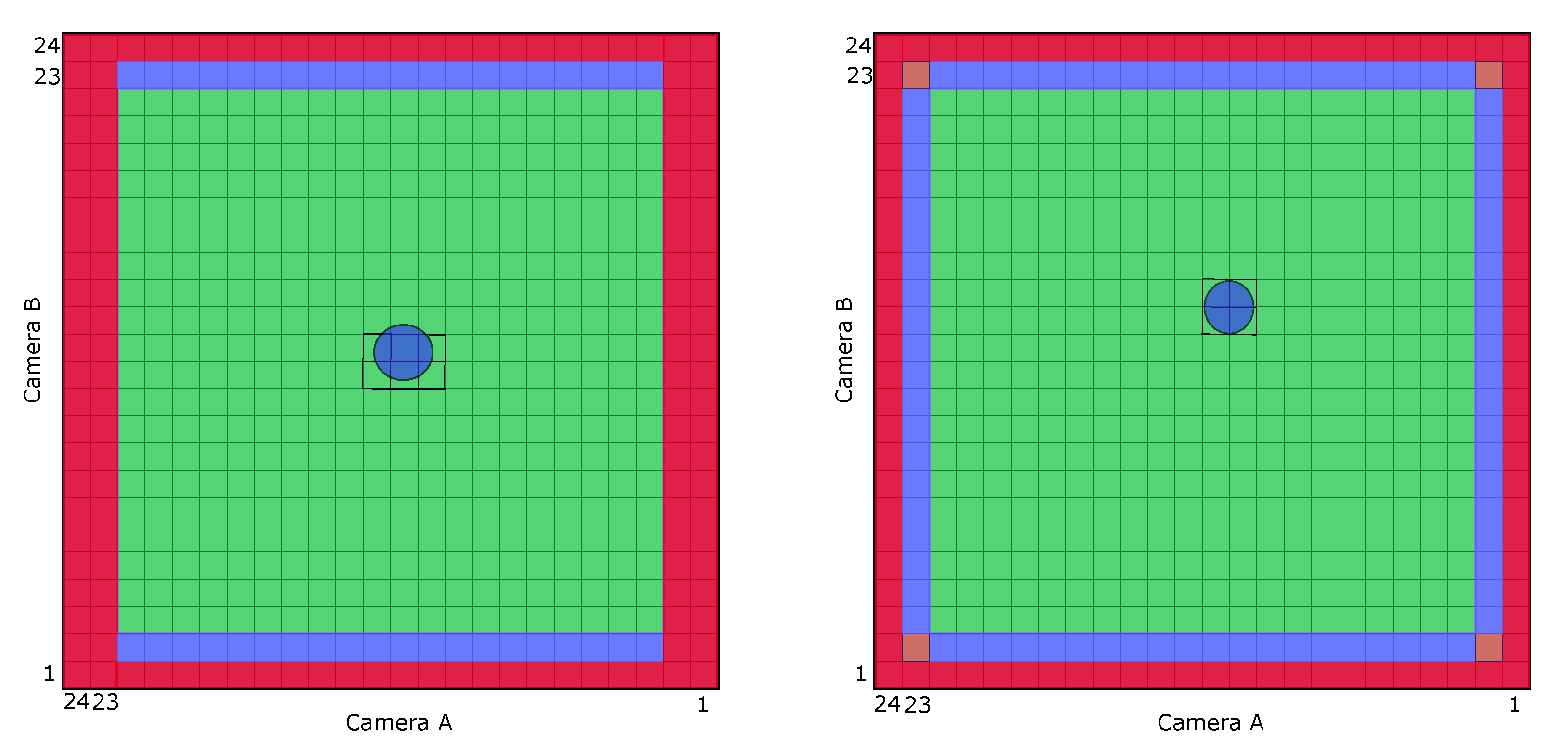
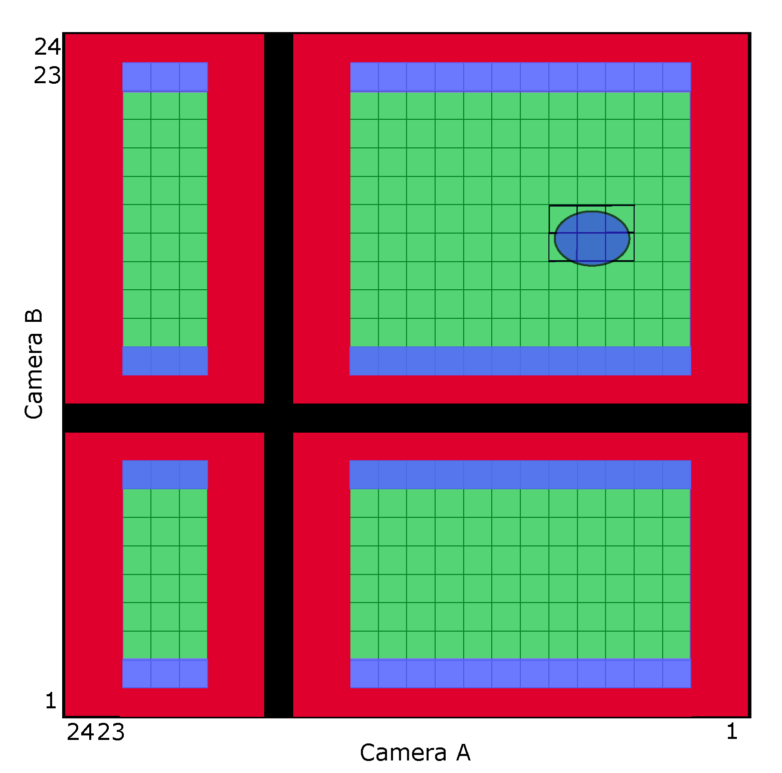
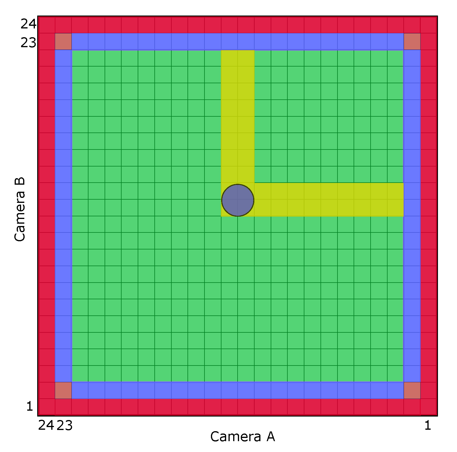
  • alistlow. This carries no information if flag2 = 0, but if flag2 = 1 it identifies the pixel numbers in camera A (if any) where drop observations appear to be anomalously missing; this helps to identify areas like the black regions in Figure 6.
  • alisthi. This carries no information if flag1 = 0, but if flag1 = 1 it identifies the pixel numbers in camera A (if any) where drop observations appear to be anomalously elevated; this also helps to identify areas like the black regions in Figure 6.
  • blistlow and blisthi–natural extensions of alistlow and alisthi for camera B.
The code sequentially looks through the list of detected drops to determine whether flag1 should trigger for each drop, then goes through all drops again to identify whether flag2 should trigger for each drop.
To identify if flag1 should trigger, the data is broken into three subsets: the first 500 drops, the “middle” of the data, and the final 500 drops.
For the first 500 drops, the collection of all shadowed pixels along both cameras for the first 1000 drops in the sample are recorded. This means that, for example, the determination if the 37th detected droplet occurs during a “flag1” anomaly depends on the detection statistics of the 36 drops before the drop and the 963 drops after the drop. This is not ideal, but allows the algorithm to use the same critical threshold for marking a statistically unlikely preponderance of drops in part of the field of view for all drops.
Determination of how many drops (out of 1000) can be identified along a single pixel of the field of view before the algorithm flags a drop with the “flag1” designation is hard-coded. The critical limit of “no more than 25 drops out of 1000 share the exact same pixel number within the extent of the shadow” was determined by running simulations of millions of drops randomly distributed within the field of view and following a realistic observed drop size distribution. Placing the limit at 25 different drops shadowing the same pixel came from looking at a 4 σ fluctuation threshold in the simulation.
For drops 501 through N 500 (where a total of N drops were observed in the day), the algorithm works the same as for the first 500 except the population of drops utilized to determine whether there is an anomaly uses a 1001 drop moving window centered on the drop in question. The final 500 drops are handled similarly to the first 500—all will have the same flag1 values based on the statistics from the final 1000 drops.
Calculation of flag2 is similar to flag1, except now the windows are 10,000 drops since these cannot be detected with acceptable statistical uncertainty with only 1000 drops. The “opening window” and “closing window” where all drops have the same flag2 values is now 5000 drops long, and the critical threshold for how few drops out of the 10,000 drop sample need to shadow a pixel to avoid labelling as anomalously low is now 27.
The variables alisthi, alistlow, blisthi, and blistlow are straightforward—the pixel numbers where the statistical limits set out in the algorithm are exceeded are recorded and assigned to the associated drop.
The condition of extrapart is found by checking whether the shadowed pixels for each drop intersect with alisthi and/or blisthi. If any of the shadows intersect alisthi and/or blisthi, then extrapart returns a value of 1; otherwise, it is 0 for the drop.
Note that this code does not detect all of the spurious drops that we remove from the data record in our analysis. The area assignment code re-explores this to take into account detected drops that may not have been explicitly in the problem region but were close enough to the problem region to be potentially mis-sized; this variable is called “extrapart2” in that code and is more aggressive in removing drops than the code being described here. All drops that have extrapart = 1 have extrapart2 = 1, but not all particles that have extrapart2 = 1 have extrapart = 1.
Versions of this algorithm that run in MATLAB are available on request.

Appendix B. Calculation of the Area of Each Pixel

This appendix focuses on the way in which the measurements presented in Table 1 can be utilized to generate a pixel area lookup table as visualized in Figure 3; this is done in three steps.
1
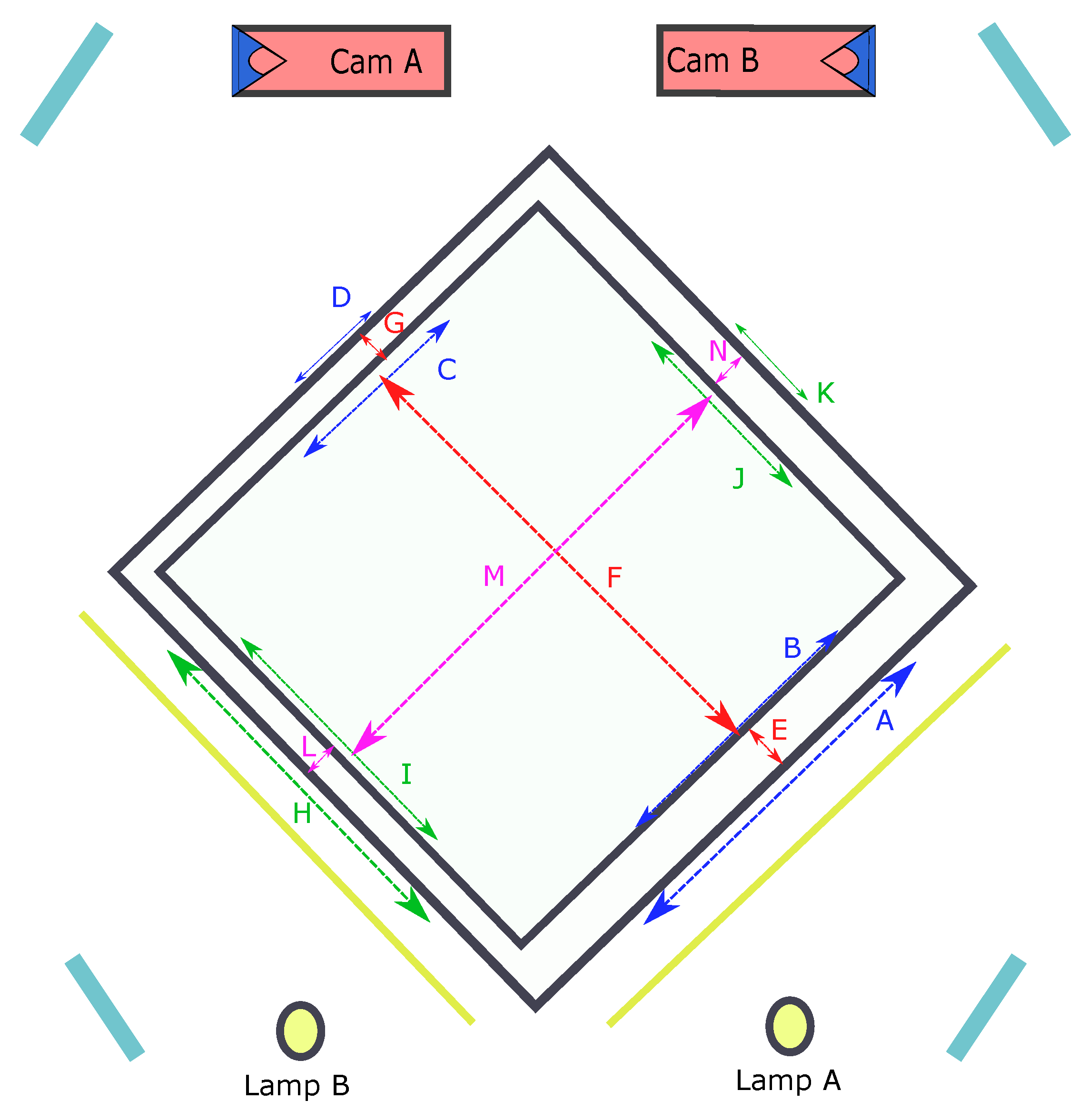
First, we define a coordinate system where the center of the field of view is set as the origin (see Figure A1). Then, using the data from Table 1, a fit is made relating the width of the field of view to the distance from the lines marked D and K on Figure 2. The light sheet linearly narrows from A to D (and H to K). Extending these lines to the focal point allows us to define the distance between the camera focal point and the center of the field of view; we label these distances as A ˜ and B ˜ , respectively.
Using basic trigonometry, the triangles that are formed by connecting these focal points to the width measurements (e.g., A, B, C, and D) give four triangles each with very similar angles near the vertex at A ˜ . We then divide that angle equally among the 632 pixels in the camera’s field of view. This angle (that we call α and β for cameras A and B, respectively) corresponds to the angle at the focal point associated with a single pixel width as it propagates back towards the illumination source.
2
From the information and coordinate system implied previously (with the origin at the center of the field of view), the coordinates A and B of each of the four corners of a given pixel are determined from the following expressions (derived again from a geometrical analysis of the layout):
A = B ˜ + A ˜ tan ( γ A ) cot ( γ B ) tan ( γ A )
B = A ˜ + B ˜ tan ( γ B ) cot ( γ A ) tan ( γ B )
where γ A and γ B are determined to be the multiples of α and β necessary to point to the appropriate corners of the pixel in question. For example, γ A = m α and γ B = n β would be used to calculate the co-ordinates of a pixel corner that is m pixels removed from the middle of the field of view of camera A and n pixels removed from the middle of the field of view of camera B (m and n are integers in the range between −316 and +316, depending on the pixel in question).
3
The coordinates of the four corners of each pixel are used to calculate the area of the resulting irregular quadrilateral. Each quadrilateral can be split into 2 scalene triangles. Let the four sides of the quadrilateral be labeled 1 , 2 , 3 , and 4 and the diagonal corresponding to the line connecting the furthest combined distance from the cameras to the closest combined distance from the cameras be labeled z. From these five distances, the total quadrilateral area can be computed via Herron’s formula as
α k = S 1 ( S 1 1 ) ( S 1 2 ) ( S 1 z ) + S 2 ( S 2 3 ) ( S 2 4 ) ( S 2 z )
where S 1 and S 2 are defined as:
S 1 = 1 + 2 + z 2
S 2 = 3 + 4 + z 2
After the value of α k is calculated for each pixel, it is stored in a lookup table indexed to position ( m , n ) for that 2DVD. Fortunately, once the lookup table is made it can be permanently stored and—so long as the optical dimensions of the 2DVD do not change—the stored lookup-table can be used to compute the area for each detected drop in that detector using Equation (3).
Figure A1. An illustration of the basic coordinate system used to find the area for each pixel, drawn for a simplified 8 pixel × 8 pixel geometry. Following the notational conventions established in the appendix, the dotted exemplar vertex corresponds to m = 3 and n = 2 .
Atmosphere 11 00855 g0a1

Appendix C. Further Considerations Related to Sensing Area

Assuming the optical field of view of the 2DVD has been measured properly, the value a i when computed with Equation (3) is designed to be directly inserted into Equation (2) and (with proper unit conversion) Equation (1).
It may sometimes be important to distinguish between the effective sample area for the drop a i and a similar but slightly different quantity we will call s ( D , t ) . The quantity s ( D , t ) is meant to represent the effective sensing area for a hypothetical drop of spherical diameter D entering the sensing volume at time t through the sensor. By definition, a i is a property of a particular drop (and, thus, implicitly a function of that drop’s properties like D i ), whereas s ( D , t ) is a function of time and is altered by the presence of any drop within the field of view of the sensor.
Consider a spherical droplet of diameter D 1 falling through the 2DVD sample area that resides in the sensing volume for the time interval t 1 to t 1 + ( Δ t ) 1 . For simplicity, assume that ( t 1 , t 1 + ( Δ t ) 1 ) occurs during a time when no other drops exist in the sample volume and there is no anomaly due to the presence of a persistent obstacle on the optics. This droplet (while being detected) temporarily renders part of the 2DVD sensing area insensitive to other drops during the (very brief) time interval that the droplet traverses the sensing region. Why? Because each detected drop casts a “shadow of insensitivity” that extends from the part of the drop closest to the camera back through the rest of the droplet and continuing back to the illumination source; a second real droplet falling through the 2DVD sensing volume at the exact same time falling within that shadow will be undetected or measured improperly. These shadows are illustrated in Figure A2. Admittedly, the “shadow of insensitivity” occurs only for the very brief time interval of duration ( Δ t ) 1 and typically obscures a very small fraction of the sensing area, but considerations involving simultaneous droplet arrivals are not unheard of in intense rain events and have been previously discussed when exploring the 2DVD’s ability to properly measure coincident droplets (e.g., see in [9]). It is also potentially noteworthy that every detected drop necessarily is detected during a time when such a shadow exists and thus s ( D , t ) is always distinct from a i during the detection of a drop.
Figure A2. A cartoon similar to Figure 4, Figure 5 and Figure 6 that shows the insensitive region during a drop detection in yellow; this “shadow area” prevents the simultaneous detection of a drop anywhere in the highlighted region. The yellow highlighted area is what is referred to as δ i in the text.
Atmosphere 11 00855 g0a2
Whereas a i has historically been used to compute rain rates, s ( D , t ) may be more appropriate to answer questions related to drop arrival rates as it is a more appropriate answer to the question “what was the effective sensing area of the detector for drops matching the diameter of the detected drop during the detection of this drop?” In case this quantity is ever needed, our revised area computation algorithm computes s ( D , t ) at the arrival time of each drop. Algorithmically, s ( D , t ) = a i δ i where δ i is the area related to the drop coverage and its shadow (as shown in Figure A2) that previously had not been subtracted from a i .

References

  1. Uijlenhoet, R.; Stricker, J. A consistent rainfall parameterization based on the exponential raindrop size distribution. J. Hydrol. 1999, 218. [Google Scholar] [CrossRef]
  2. Gage, K.; Williams, C.; Clark, W.; Johnston, P.; Carter, D. Profiler contributions to tropical rainfall measuring mission (TRMM) ground validation field campaigns. J. Atmos. Ocean. Technol. 2002, 19, 843–863. [Google Scholar] [CrossRef]
  3. Datta, S.; Jones, W.; Roy, B.; Tokay, A. Spatial variability of surface rainfall as observed from TRMM field campaign data. J. Appl. Meteorol. 2003, 42, 598–610. [Google Scholar] [CrossRef] [Green Version]
  4. Miriovsky, B.; Bradley, A.; Eichinger, W.; Krajewski, W.; Kruger, A.; Nelson, B.; Creutin, J.D.; Lapetite, J.M.; Lee, G.; Zawadzki, I.; et al. An experimental study of small-scale variability of radar reflectivity using disdrometer observations. J. Appl. Meteorol. 2004, 43, 106–118. [Google Scholar] [CrossRef]
  5. Krajewski, W.; Kruger, A.; Caracciolo, C.; Golé, P.; Barthes, L.; Creutin, J.D.; Delahaye, J.Y.; Nikolopoulos, E.; Ogden, F.; Vinson, J.P. DEVEX-disdrometer evaluation experiment: Basic results and implications for hydrologic studies. Adv. Water Resour. 2006, 29, 807–814. [Google Scholar] [CrossRef]
  6. Jensen, M.; Petersen, W.; Bansemer, A.; Bharadwaj, N.; Carey, L.; Cecil, D.; Collis, S.; DelGenio, A.; Dolan, B.; Gerlach, J.; et al. The midlatitude continental convective clouds experiment (MC3E). Bull. Am. Meteorol. Soc. 2016, 97, 1667–1686. [Google Scholar] [CrossRef]
  7. Roberto, N.; Adirosi, E.; Baldini, L.; Casella, D.; Dietrich, S.; Gatlin, P.; Panegrossi, G.; Petracca, M.; Sanò, P.; Tokay, A. Multi-sensor analysis of convective activity in central Italy during the HyMeX SOP 1.1. Atmos. Meas. Tech. 2016, 9, 535–552. [Google Scholar] [CrossRef] [Green Version]
  8. Kathiravelu, G.; Lucke, T.; Nichols, P. Rain Drop Measurement Technologies: A Review. Water 2016, 8, 29. [Google Scholar] [CrossRef] [Green Version]
  9. Kruger, A.; Krajewski, W. Two-Dimensional Video Disdrometer: A Description. J. Atmos. Ocean. Technol. 2002, 19, 602–617. [Google Scholar] [CrossRef]
  10. Schönhuber, M.; Lammer, G.; Randeu, W. The 2D video disdrometer. In Precipitation: Advances in Measurement, Estimation and Prediction; Michaelides, S., Ed.; Springer: Berlin/Heidelberg, Germany, 2008; pp. 3–31. [Google Scholar]
  11. Gage, K.; Williams, C.; Johnston, P.; Ecklund, W.; Cifelli, R.; Tokay, A.; Carter, D. Doppler radar profilers as calibration tools for scanning radars. J. Appl. Meteorol. 2000, 39, 2209–2222. [Google Scholar] [CrossRef]
  12. Williams, C.; Kruger, A.; Gage, K.; Tokay, A.; Cifelli, R.; Krajewski, W.; Kummerow, C. Comparison of simultaneous rain drop size distributions estimated from two surface disdrometers and a UHF profiler. Geophys. Res. Lett. 2000, 27, 1763–1766. [Google Scholar] [CrossRef] [Green Version]
  13. Tokay, A.; Kruger, A.; Krajewski, W. Comparison of drop size distribution measurements by impact and optical disdrometers. Adv. Geosci. 2001, 30, 3–9. [Google Scholar] [CrossRef]
  14. Bringi, V.; Chandrasekar, V.; Hubbert, J.; Gorgucci, E.; Randeu, W.; Schönhuber, M. Raindrop size distribution in different climatic regions from disdrometer and dual-polarized radar analysis. J. Atmos. Sci. 2003, 60, 354–365. [Google Scholar] [CrossRef]
  15. Thurai, M.; Bringi, V. Drop axis ratios from a 2D video disdrometer. J. Atmos. Ocean. Technol. 2005, 22, 966–978. [Google Scholar] [CrossRef]
  16. Cao, Q.; Zhang, G.; Brandes, E.; Schuur, T.; Ryzhkov, A.; Ikeda, K. Analysis of video disdrometer and polarimetric radar data to characterize rain microphysics in Oklahoma. J. Appl. Meteorol. Climatol. 2008, 47, 2238–2255. [Google Scholar] [CrossRef] [Green Version]
  17. Cao, Q.; Zhang, G. Errors in estimating raindrop size distribution parameters employing disdrometer and simulated raindrop spectra. J. Appl. Meteorol. Climatol. 2009, 48, 406–425. [Google Scholar] [CrossRef]
  18. Yoshikawa, E.; Kida, S.; Yoshida, S.; Morimoto, T.; Ushio, T.; Kawasaki, Z. Vertical structure of raindrop size distribution in lower atmospheric boundary layer. Geophys. Res. Lett. 2010, 37, L20802. [Google Scholar] [CrossRef]
  19. Thurai, M.; Petersen, W.; Tokay, A.; Shultz, C.; Gatlin, P. Drop size distribution comparisons between Parsivel and 2-D video disdrometers. Adv. Geosci. 2011, 30, 3–9. [Google Scholar] [CrossRef] [Green Version]
  20. Marzuki; Randeu, W.; Kozu, T.; Simonmai, T.; Hashiguchi, H.; Schönhuber, M. Raindrop axis ratios, fall velocities and size distribution over Sumatra from 2D-Video Disdrometer measurement. Atmos. Res. 2013, 119, 23–37. [Google Scholar] [CrossRef]
  21. Tokay, A.; Petersen, W.; Gatlin, P.; Wingo, M. Comparison of raindrop size distribution measurements by collocated disdrometers. J. Atmos. Ocean. Technol. 2013, 30, 1672–1690. [Google Scholar] [CrossRef]
  22. Adirosi, E.; Gorgucci, E.; Baldini, L.; Tokay, A. Evaluation of Gamma raindrop size distribution assumption through comparison of rain rates of measured and radar-equivalent Gamma DSD. J. Appl. Meteorol. Climatol. 2014, 53, 1618–1635. [Google Scholar] [CrossRef]
  23. Ferretti, G.; Pichelli, E.; Gentile, S.; Maiello, I.; Cimini, D.; Davolio, S.; Miglietta, M.; Panegrossi, G.; Baldini, L.; Pasi, F.; et al. Overview of the first HyMeX special observation period over Italy: Observations and model results. Hydrol. Earth Syst. Sci. 2014, 18, 1953–1977. [Google Scholar] [CrossRef] [Green Version]
  24. Larsen, M.; Kostinski, A.; Jameson, A. Further evidence for super-terminal raindrops. Geophys. Res. Lett. 2014, 41, 6914–6918. [Google Scholar] [CrossRef] [Green Version]
  25. Gatlin, P.; Thurai, M.; Bringi, V.; Petersen, W.; Wolff, D.; Tokay, A.; Carey, L.; Wingo, M. Searching for large raindrops: A global summary of two-dimensional video disdrometer observations. J. Appl. Meteorol. Climatol. 2015, 54, 1069–1088. [Google Scholar] [CrossRef]
  26. Gires, A.; Tchiguirinskaia, I.; Schertzer, D.; Berne, A. 2DVD Data Revisited: Multifractal insights into cuts of the spatiotemporal rainfall process. J. Hydrometeorol. 2015, 16, 548–562. [Google Scholar] [CrossRef] [Green Version]
  27. Raupach, T.; Berne, A. Correction of raindrop size distributions measured by Parsivel disdrometers, using a two-dimensional video disdrometer as a reference. Atmos. Meas. Tech. 2015, 8. [Google Scholar] [CrossRef] [Green Version]
  28. Adirosi, E.; Volpi, E.; Lombardo, F.; Baldini, L. Raindrop size distribution: Fitting performance of common theoretical models. Adv. Water Resour. 2016, 96, 290–305. [Google Scholar] [CrossRef]
  29. Adirosi, E.; Baldini, L.; Roberto, N.; Gatlin, P.; Tokay, A. Improvement of vertical profiles of raindrop size distribution from micro rain radar using 2D video disdrometer measurements. Atmos. Res. 2016, 169, 404–415. [Google Scholar] [CrossRef]
  30. Jameson, A.; Larsen, M.; Kostinski, A. An example of persistent microstructure in a long rain event. J. Hydrometeorol. 2016, 17, 1661–1673. [Google Scholar] [CrossRef]
  31. Jameson, A.; Larsen, M. Estimates of the statistical two-dimensional spatial structure in rain over a small network of disdromters. Meteorol. Atmos. Phys. 2016, 128, 401–413. [Google Scholar] [CrossRef] [Green Version]
  32. Jameson, A.; Larsen, M. The variability of rainfall rate as a function of area. J. Geophys. Res. Atmos. 2016, 121. [Google Scholar] [CrossRef] [Green Version]
  33. Larsen, M.; O’Dell, K. Sampling variability effects in drop-resolving disdrometer observations. J. Geophys. Res. Atmos. 2016, 121. [Google Scholar] [CrossRef]
  34. Thurai, M.; Gatlin, P.; Bringi, V. Separating stratiform and convective rain types based on the drop size distribution characteristics using 2D video disdrometer data. Atmos. Res. 2016, 169, 416–423. [Google Scholar] [CrossRef]
  35. Park, S.G.; Kim, H.L.; Ham, Y.W.; Jung, S.H. Comparative evaluation of the OTT PARSIVEL2 using a collocated two-dimensional video disdrometer. J. Atmos. Ocean. Technol. 2017, 34, 2059–2082. [Google Scholar] [CrossRef]
  36. Tokay, A.; D’Adderio, L.; Porcù, F.; Wolff, D.; Petersen, W. A field study of footprint-scale variability of raindrop size distribution. J. Hydrometeorol. 2017, 18, 3165–3179. [Google Scholar] [CrossRef]
  37. Wen, G.; Xiao, H.; Yang, H.; Bi, Y.; Xu, W. Characteristics of summer and winter precipitation over northern China. Atmos. Res. 2017, 197, 390–406. [Google Scholar] [CrossRef]
  38. Wen, L.; Zhao, K.; Zhang, G.; Liu, S.; Chen, G. Impacts of instrument limitations on estimated raindrop size distribution, radar parameters, and model microphysis during Mei-Yu season in east China. J. Atmos. Ocean. Technol. 2017, 34, 1021–1037. [Google Scholar] [CrossRef]
  39. Adirosi, E.; Roberto, N.; Montopoli, M.; Gorgucci, E.; Baldini, L. Influence of disdrometer type on weather radar algorithms from measured DSD: Application to Italian Climatology. Atmosphere 2018, 9, 360. [Google Scholar] [CrossRef] [Green Version]
  40. Bringi, V.; Thurai, M.; Baumgardner, D. Raindrop fall velocities from an optical array probe and 2-D video disdrometer. Atmos. Meas. Tech. 2018, 11, 1377–1384. [Google Scholar] [CrossRef] [Green Version]
  41. D’Adderio, L.; Porcù, F.; Tokay, A. Evolution of drop size distribution in natural rain. Atmos. Res. 2018, 200, 70–76. [Google Scholar] [CrossRef]
  42. Larsen, M.; Schönhuber, M. Identification and characterization of an anomaly in 2-dimensional video disdrometer data. Atmosphere 2018, 9, 315. [Google Scholar] [CrossRef] [Green Version]
  43. Liu, X.; Wan, Q.; Wang, H.; Xiao, H.; Zhang, Y.; Zheng, T.; Feng, L. Raindrop size distribution parameters retrieved from Guangzhou S-band polarimetric radar observations. J. Meteorol. Res. 2018, 32, 571–583. [Google Scholar] [CrossRef]
  44. Manić, S.; Thurai, M.; Bringi, V.; Notarosš, B. Scattering calculations for asymmetric raindrops during a line convection event: Comaprison with Radar measurements. J. Atmos. Ocean. Technol. 2018, 35, 1169–1180. [Google Scholar] [CrossRef]
  45. Thurai, M.; Bringi, V. Application of the generalized gamma model to represent the full rain drop size distribution spectra. J. Appl. Meteorol. Climatol. 2018, 57, 1197–1210. [Google Scholar] [CrossRef]
  46. Wen, L.; Zhao, K.; Chen, G.; Wang, M.; Zhou, B.; Huang, H.; Hu, D.; Lee, W.C.; Hu, H. Drop size distribution characteristics of seven typhoons in China. J. Geophys. Res. Atmos. 2018, 123, 6529–6548. [Google Scholar] [CrossRef]
  47. Liu, X.; He, B.; Zhao, S.; Hu, S.; Liu, L. Comparative measurement of rainfall with a precipitation micro-physical characteristics sensor, a 2D video disdrometer, an OTT PARSIVEL disdrometer, and a rain gauge. Atmos. Res. 2019, 229, 100–114. [Google Scholar] [CrossRef]
  48. Mahale, V.; Guifu, Z.; Ming, X.; Jidong, G.; Reeves, H. Variational retrieval of rain microphysics and related parameters from polarimetric radar data with a parameterized operator. J. Atmos. Ocean. Technol. 2019, 36, 2483–2500. [Google Scholar] [CrossRef]
  49. Raupach, T.; Thurai, M.; Bringi, V.; Berne, A. Reconstructing the drizzle mode of the raindrop size distribution using double-moment normalization. J. Appl. Meteorol. Climatol. 2019, 58, 145–164. [Google Scholar] [CrossRef]
  50. Thurai, M.; Bringi, V.; Gatlin, P.; Petersen, W.; Wingo, M. Measurements and modeling of the full rain drop size distribution. Atmosphere 2019, 10, 39. [Google Scholar] [CrossRef] [Green Version]
  51. Conrick, R.; Zagrodnik, J.; Mass, C. Dual-polarization radar retrievals of coastal pacific northwest raindrop size distribution parameters using random forest regression. J. Atmos. Ocean. Technol. 2020, 37, 229–242. [Google Scholar] [CrossRef]
  52. Das, S.; Simon, S.; Kolte, Y.; Krishna, U.; Deshpande, S.; Hazra, A. Investigation of raindrops fall velocity during different monsoon seasons over the Western Ghats, India. Earth Space Sci. 2020, 7. [Google Scholar] [CrossRef] [Green Version]
  53. Luo, L.; Xiao, H.; Yang, H.; Chen, H.; Guo, J.; Sun, Y.; Feng, L. Raindrop size distribution and microphysical characteristics of a great rainstorm in 2016 in Beijing, China. Atmos. Res. 2020, 239, 104895. [Google Scholar] [CrossRef]
  54. Thurai, M.; Steger, S.; Teschl, F.; Schönhuber, M. Analysis of raindrop shapes and scattering calculations: The outer rain bands of tropical depression Nate. Atmosphere 2020, 11, 114. [Google Scholar] [CrossRef] [Green Version]
  55. Tokay, A.; D’Adderio, L.; Marks, D.; Pippitt, J.; Wolff, D.; Patersen, W. Comparison of raindrop size distribution between NASA’s S-Band Polarimetric Radar and Two-Dimensional Video Disdrometers. J. Appl. Meteorol. Climatol. 2020, 59, 517–533. [Google Scholar] [CrossRef]
  56. Tokay, A.; D’Adderio, L.; Wolff, D.; Petersen, W. Development and evaluation of the raindrop size distribution parameters for the NASA Global Precipitation Measurement Mission ground validation program. J. Atmos. Ocean. Technol. 2020, 37, 115–128. [Google Scholar] [CrossRef]
  57. Zhou, L.; Dong, X.; Fu, Z.; Wang, B.; Leng, L.; Xi, B.; Cui, C. Vertical distributions of raindrops and Z-R relationships using microrain radar and 2-D-Video Distrometer Measurements During the Integrative Monsoon Frontal Rainfall Experiment (IMFRE). J. Geophys. Res. Atmos. 2020, 125, e2019JD031108. [Google Scholar] [CrossRef] [Green Version]
  58. Löffler-Mang, M.; Joss, J. An optical disdrometer for measuring size and velocity of hydrometeors. J. Atmos. Ocean. Technol. 2000, 17, 130–139. [Google Scholar] [CrossRef]
  59. Battaglie, A.; Rustemeier, E.; Tokay, A.; Blahak, U.; Simmer, C. PARSIVEL snow observations: A cricital assessment. J. Atmos. Ocean. Technol. 2010, 27, 333–344. [Google Scholar] [CrossRef]
  60. Nespor, V.; Krajewski, W.; Kruger, A. Wind-induced error of raindrop size distribution measurement using a two-dimensional video disdrometer. J. Atmos. Ocean. Technol. 2000, 17, 1483–1492. [Google Scholar] [CrossRef]
  61. Schönhuber, M.; Lammer, G.; Randeu, W. One decade of imaging precipitation measurement by 2D-video-distrometer. Adv. Geosci. 2007, 10, 85–90. [Google Scholar] [CrossRef] [Green Version]
  62. Angulo-Martinez, M.; Begueria, S.; Latorre, B.; Fernández-Raga, M. Comparison of precipitation measurements by OTT Parsivel2 and Thies LPM optical disdrometers. Hydrol. Earth Syst. Sci. 2018, 22, 2811–2837. [Google Scholar] [CrossRef] [Green Version]
  63. Frasson, R.; da Cunha, L.; Krajewski, W. Assessment of the Thies optical disdrometer performance. Atmos. Res. 2011, 101, 237–255. [Google Scholar] [CrossRef]
  64. Liu, X.; Gao, T.; Liu, L. A comparison of rainfall measurements from multiple instruments. Atmos. Meas. Tech. 2013, 6, 1585–1595. [Google Scholar] [CrossRef] [Green Version]
  65. Das, S.; Konwar, M.; Chakravarty, K.; Deshpande, S. Raindrop size distribution of different cloud types over the Western Ghats using simultaneous measurements from Micro-Rain Radar and disdrometer. Atmos. Res. 2017, 186, 72–82. [Google Scholar] [CrossRef]
  66. Wen, L.; Zhao, K.; Zhang, G.; Xue, M.; Zhou, B.; Liu, S.; Chen, X. Statistical characteristics of raindrop size distributions observed in East China during the Asian summer monsoon season usign 2-D video disdrometer and Micro Rain Radar data. J. Geophys. Res. Atmos. 2016, 121, 2265–2282. [Google Scholar] [CrossRef] [Green Version]
  67. Chang, W.; Lee, G.; Jou, B.D.; Lee, W.C.; Lin, P.L.; You, C.K. Uncertainty in measured raindrop size distributions from four types of collocated instruments. Remote Sens. 2020, 12, 1167. [Google Scholar] [CrossRef] [Green Version]
  68. Jameson, A.; Larsen, M.; Kostinski, A. Disdrometer network observations of finescale spatial-temporal clustering in rain. J. Atmos. Sci. 2015, 72, 1648–1666. [Google Scholar] [CrossRef] [Green Version]
  69. Kostinski, A.; Jameson, A. Fluctuation properties of precipitation. Part I: On deviations of single-size drop counts from the Poisson distribution. J. Atmos. Sci. 1997, 54, 2174–2186. [Google Scholar] [CrossRef]
  70. Jameson, A.; Kostinski, A. Fluctuation properties of precipitation. Part IV: Finescale clustering of drops in variable rain. J. Atmos. Sci. 1999, 56, 82–91. [Google Scholar] [CrossRef]
  71. Uijlenhoet, R. Parameterization of Rainfall Microstructure for Radar Meteorology and Hydrology. Ph.D. Thesis, Wageningen University, Wageningen, The Netherlands, 1999. [Google Scholar]
  72. Marzuki; Randeu, W.; Schönhuber, M.; Bringi, V.; Kozu, T.; Shimomai, T. Raindrop size distribution parameters of disdrometer data with different bin sizes. IEEE Trans. Geosci. Remote Sens. 2010, 48, 3075–3080. [Google Scholar] [CrossRef]
  73. Marzuki; Randeu, W.; Kozu, T.; Shimomai, T.; Schönhuber, M.; Hashiguchi, H. Estimation of raindrop size distribution parameters by maximum likelihood and L-moment methods: Effect of discretization. Atmos. Res. 2012, 112, 1–11. [Google Scholar] [CrossRef]
  74. Liu, X.; Gao, T.; Hu, Y.; Shi, X. Measuring hydrometeors using a preciptation microphysical characteristics sensor: Sampling effect of different bin sizes on drop size distribution parameters. Adv. Meteorol. 2018, 2018, 9727345. [Google Scholar] [CrossRef] [Green Version]
Figure 1. The left panel shows an exaggerated cartoon of a top-down view of the 2DVD measurement area geometry; for simplicity, the intersection of the cameras is shown as if each line scan camera is composed of only 3 pixels, whereas the line scan cameras in an actual 2DVD have 632 pixels on a side. The right panel shows a remapping of this measurement region (which is actually the intersection of two trapezoids) into a regular square grid. Though the square grid is more convenient for visualization, note that the true areas of pixels A and I are physically different when accounting for the real optical geometry (which becomes relevant when determining the drop size-dependent effective sample area).
Atmosphere 11 00855 g001
Figure 2. A top-down cartoon displaying the measurements characterizing the optical field of view for each 2DVD. Light rays traverse through the interior of the instrument diagonally, traveling from each lamp to the adjacent (light blue) mirror, propagating through the (yellow) Fresnel lens and (through slits in a metal frame) into the interior of the measurement area. The light then propagates through slits on the other side of the measurement area to the mirror next to the associated camera. All labeled distances in the figure were carefully measured at the field site. If the pixels in the field of view really would be of uniform size, then the distances marked A, B, C, and D would all be the same length (as would H, I, J, and K). Actual measurements for both 2DVDs used in this study are shown in Table 1.
Atmosphere 11 00855 g002
Figure 3. The effective area (in mm 2 ) of each pixel within the field of view for 2DVD SN074, as determined by using the measurements presented in Table 1. The geometry is shown to coincide with the orientation presented in Figure 2.
Atmosphere 11 00855 g003
Figure 4. A cartoon showing how the effective sample area should be calculated for a drop covering 3 pixels along both camera axes. Pixels colored red are places that the droplet center could not have fallen and been successfully detected by the 2DVD, whereas pixels colored green show places that the droplet center could have been located and still had the 1 pixel of unshadowed area necessary to detect and properly size the drop.
Atmosphere 11 00855 g004
Figure 5. Similar to Figure 4, this shows the same drop falling in different locations so that it covers a 2 × 3 and 2 × 2 block of pixels, respectively. A pixel is only considered shadowed if the majority of a pixel is covered, so the left hand panel shadows a 2 × 3 region—not a 3 × 3 region. Blue shading near the boundary indicates pixels that should have half of their area included in the effective sample area computation, and orange coloring indicates pixels that should only have one fourth of their area included.
Atmosphere 11 00855 g005
Figure 6. A cartoon of the sample area calculation of a 24 × 24 pixel domain for a 3 × 2 pixel drop detected during a time of partial instrumental insensitivity. Pixel coloring is the same as used in Figure 4 and Figure 5. Additional area is removed from the sample area due to the presence of two simultaneous anomalies (shown in black). As before, the effective sample area for this drop would be calculated by adding the areas of all green pixels with half the areas of all blue pixels.
Atmosphere 11 00855 g006
Figure 7. The frequency of accumulation ratios between the corrected and raw daily data sets in the ensemble; a value of 1.1 suggests that the corrected accumulation is 10% larger than the original reported accumulation. Small net corrections of less than 5% appear typical.
Atmosphere 11 00855 g007
Figure 8. Rain Rate (based on 1 min time-binning) for 2DVD SN074 on 18 February 2020. The “combined correction” incorporates both removal of the spurious drops and the adjustment of the detector effective-area.
Atmosphere 11 00855 g008
Figure 9. A sub-interval of the rain rates shown in Figure 8. In addition to the raw data and the “combined correction” results, the rain rates looking at each correction individually are shown.
Atmosphere 11 00855 g009
Figure 10. A different way to visualize the results seen in Figure 8. The ratio between the corrected rain rate ( R adj ) and the rain rate estimated from the uncorrected data record ( R raw ) plotted against the corrected rain rate R adj .
Atmosphere 11 00855 g010
Figure 11. A histogram showing the ratio between the adjusted area and the manufacturer-reported area for all of the non-spurious drops retained in the ensemble. Note that all adjusted areas are at least 6% smaller than the manufacturer-reported areas in the output file of the 2DVD.
Atmosphere 11 00855 g011
Table 1. The measurements used for determining the pixel sizes within the field of view; the letters in the “measurement” field correspond to the labels shown in Figure 2. All measurements are given to nominal 1 mm resolution. All distances were measured at least 3 times by at least 2 different people on different days and reported values within ∼0.5 mm of each other.
Measurement2DVD SN0742DVD SN098Measurement2DVD SN0742DVD SN098
A134.3 mm132.8 mmH134.0 mm131.7 mm
B126.1 mm125.2 mmI126.6 mm124.1 mm
C78.1 mm78.6 mmJ79.2 mm77.9 mm
D70.2 mm70.9 mmK71.4 mm70.8 mm
E40.1 mm39.6 mmL39.7 mm39.9 mm
F291.3 mm291.0 mmM291.3 mm289.0 mm
G40.4 mm40.3 mmN40.0 mm40.4 mm
Table 2. Summary of ensemble data under different processing paradigms. The entire data set had 202,555,318 total drops, of which 194,089,999 were retained after removing spurious drops. D indicates mean diameter whereas D m specifies mass-weighted mean diameter. When binned, constant bin widths of 0.2 mm were used. Low-Bin indicates reported diameters were rounded down to the lower bound of the associated diameter bin, whereas mid-bin assigned drop diameters at the midpoint of the associated bin.
Spurious DropsAreaDiameterTotal Accum. D D m
RemovedFixedBinningDepth (mm)(mm)(mm)
None7046.90.5810.888
NNLow-Bin5735.00.4800.829
Mid-Bin7177.20.5800.894
None7900.40.5810.888
NYLow-Bin6449.40.4800.829
Mid-Bin8042.50.5800.894
None6560.40.5790.880
YNLow-Bin5322.50.4790.820
Mid-Bin6684.30.5790.886
None7124.30.5790.880
YYLow-Bin5780.90.4790.820
Mid-Bin7258.70.5790.886

