Trends of UV Radiation in Antarctica


1
Biospherical Instruments Inc., San Diego, CA 92110, USA
2
NOAA Global Monitoring Laboratory, Boulder, CO 80305, USA
*
Author to whom correspondence should be addressed.
Atmosphere 2020, 11(8), 795; https://doi.org/10.3390/atmos11080795
Submission received: 1 July 2020
/
Revised: 23 July 2020
/
Accepted: 23 July 2020
/
Published: 28 July 2020
(This article belongs to the Special Issue Ozone and Stratospheric Dynamics)
Abstract
:The success of the Montreal Protocol in curbing increases in harmful solar ultraviolet (UV) radiation at the Earth’s surface has recently been demonstrated. This study also provided evidence that the UV Index (UVI) measured by SUV-100 spectroradiometers at three Antarctic sites (South Pole, Arrival Heights, and Palmer Station) is now decreasing. For example, a significant (95% confidence level) downward trend of −5.5% per decade was reported at Arrival Heights for summer (December through February). However, it was also noted that these measurements are potentially affected by long-term drifts in calibrations of approximately 1% per decade. To address this issue, we have reviewed the chain of calibrations implemented at the three sites between 1996 and 2018 and applied corrections for changes in the scales of spectral irradiance (SoSI) that have occurred over this period (Method 1). This analysis resulted in an upward correction of UVI data measured after 2012 by 1.7% to 1.8%, plus smaller adjustments for several shorter periods. In addition, we have compared measurements during clear skies with model calculations to identify and correct anomalies in the measurements (Method 2). Corrections from both methods reduced decadal trends in UVI on average by 1.7% at the South Pole, 2.1% at Arrival Heights, and 1.6% at Palmer Station. Trends in UVI calculated from the corrected dataset are consistent with concomitant trends in ozone. The decadal trend in UVI calculated from the corrected dataset for summer at Arrival Heights is −3.3% and is significant at the 90% level. Analysis of spectral irradiance measurements at 340 nm suggests that this trend is partially caused by changes in sea ice cover adjacent to the station. For the South Pole, a significant (95% level) trend in UVI of −3.9% per decade was derived for January. This trend can partly be explained by a significant positive trend in total ozone of about 3% per decade, which was calculated from SUV-100 and Dobson measurements. Our study provides further evidence that UVIs are now decreasing in Antarctica during summer months. Reductions have not yet emerged during spring when the ozone hole leads to large UVI variability.
1. Introduction
Following the landmark paper by Molina and Rowland [1], it was clear by the mid-1980s that chlorofluorocarbons (CFCs) and other chemicals deplete the ozone layer [2]. Such decreases in stratospheric ozone will lead to increases in UV radiation at the Earth’s surface with adverse effects on human health and the environment [3,4,5,6,7,8,9]. In 1985, dramatic losses of stratospheric ozone were reported over Antarctica in the springtime [10] and were soon linked to CFCs and other ozone-depleting substances (ODSs) released into the atmosphere. This phenomenon—now commonly called the “ozone hole”—galvanized scientists, the public, and policymakers to put regulations in place to curb the emissions of ODSs, and it led to the adoption of the Montreal Protocol (MP) on Substances that Deplete the Ozone Layer in 1987 [11]. It has been shown that the MP and its subsequent amendments and adjustments have prevented catastrophic losses in stratospheric ozone. For example, modeling studies have projected that 67% of the globally averaged ozone column would have been destroyed without the MP by 2065 in comparison to 1980 [12]. This decline in ozone would have more than doubled the erythemal (sunburning) UV radiation at northern summer mid-latitudes by 2060 [13]. By 2100, the peak UV index (UVI) at mid-latitudes would have increased by a factor of four and by much larger factors at higher latitudes [14].
The discovery of the ozone hole in 1985 and concerns about increases in UV-B radiation also led to the establishment of a network of instruments for monitoring UV radiation in Antarctica [15]. This paper discusses trends in erythemal UV radiation derived from measurements of this network for the period 1996–2018.
Thanks to the MP, present-day (2014–2017) total ozone columns (TOCs) are lower than the 1964–1980 columns by only about 3.0% in the Northern Hemisphere and 5.5% in the Southern Hemisphere [16]. Concomitant increases in erythemal UV radiation have also been limited to a few percent [3]. While changes in ozone and UV radiation at Antarctica have been much larger, evidence is now emerging that the ozone hole is recovering. The most significant increases in Antarctic stratospheric ozone have been observed during September [16]. For example, Solomon et al. [17] found a positive TOC trend at the South Pole of 2.5 ± 1.5 Dobson Units (DU) per year (90% confidence level). This trend was derived from measurements of ozonesondes performed in the month of September between 2000 and 2014. This analysis was corroborated by Kuttippurath and Nair [18], who found a positive trend (95% confidence level) in the TOC of 3.68 ± 1.73 DU per year (1.72 ± 0.81% per year) for locations inside the polar vortex (≥65° S equivalent latitude as defined by Nash et al. [19]). Their data analysis is based on the average TOC over the months of September, October, and November, and for the period 2001–2013.
Detection of recovery in ultraviolet (UV) radiation over Antarctica is more difficult because it is not only affected by ozone but also additional factors such as clouds, albedo, and aerosols. McKenzie et al. [14] have assessed changes in the UVI between 1996 and 2018 at 17 locations around the world, ranging from Greenland in the North to three sites in Antarctica: South Pole, Arrival Heights, and Palmer Station. The study concluded that UVIs measured at the three Antarctic sites decreased by about 5% per decade during summer. However, only the trend at Arrival Heights is significant at the 95% confidence level. The study also cautioned that “measurements at these three remote sites are potentially affected by long-term drifts of approximately 1% per decade, which are associated with hardware modifications and changes in calibration standards,” but it concluded that “the downward trend at Arrival Heights would remain statistically significant even if these drifts were confirmed.”
It is the objective of our study to address the issues raised by McKenzie et al. [14] and to quantify the effects of changes in hardware and calibration standards on UV measurements at the three Antarctic sites. Then, we develop corrections to account for these changes and recalculate UVI trends based on the corrected datasets.
Measurements of UV radiation at the South Pole, Arrival Heights, and Palmer Station commenced at the end of the 1980s when the National Science Foundation’s (NSF) Office of Polar Programs established the Ultraviolet Spectral Irradiance Monitoring Network (UVSIMN) ([15]; http://uv.biospherical.com). The network was operated by Biospherical Instruments Inc (BSI). It remained in operation until 2009 when the instruments were transferred to the National Oceanic and Atmospheric Administration (NOAA) and became NOAA’s Antarctic UV Monitoring Network [20]. The methods of network operation and data processing employed by the NSF/BSI and NOAA networks are identical, and the combined data record constitutes the longest time series of UV radiation measurements that exists for Antarctica. A climatology of UV radiation derived from these data was assembled by Bernhard et al. [21].
Maintaining consistent measurements over a multi-decade timeframe is a demanding task. Challenges include changes in the scale of spectral irradiance (SoSI) distributed by standards laboratories (in our case the U.S. National Institute of Standards and Technology (NIST)); drift of calibration standards over time; change in hardware (instrument upgrades, replacement of defective components, small modifications prompted by regular instrument service); change in software and observation protocols (e.g., change from one to four scans per hour in 1997); changes in post-processing algorithms; personnel turn-over (and the concomitant loss of knowledge); disruptions in funding; and change of responsibility (in our case, the transfer from the NSF to NOAA). While some of these challenges cannot be easily addressed, some can be controlled, for example, by keeping rigorous documentation.
The paper is organized as follows: In Section 2, we describe the conditions at the three Antarctic sites (Section 2.1); the spectroradiometers used at these sites (Section 2.2); the methods to convert the instrument’s raw data to measurements of UV radiation (Section 2.3); the traceability of the SoSI applied to solar measurements (Section 2.4); the implications of drifts in calibration standards (Section 2.5); a method to use radiative transfer model calculations to detect and correct drifts in calibration (Section 2.6); and the method of calculating trends (Section 2.7). In Section 3, we calculate trends in the UVI from measurements at the three Antarctic sites, taking into account the corrections developed in Section 2. Then, we compare these trends with those published by McKenzie et al. [14]. In Section 4, we discuss the results of our study in a larger context and end with conclusions resulting from our work (Section 5).
2. Materials and Methods
2.1. Network Sites
Locations discussed in this study include the South Pole (90° S, 2835 m a.s.l.), Arrival Heights (77.830° S, 166.663° E, 190 m a.s.l.), and Palmer Station (64.774° S, 64.051° W, 20 m a.s.l.). All sites are greatly affected by the ozone hole.
Conditions at the South Pole are characterized by frequent cloudless days, constant high surface albedo of about 0.98 [22], little aerosol influence, negligible air pollution apart from local sources, and virtually no diurnal change in the solar zenith angle (SZA). The high albedo greatly suppresses the effects of clouds [23]. As a result, spectral irradiance at 347.5 nm is almost never reduced to less than 80% of the clear-sky intensity [24]. The instrument is located in the Atmospheric Research Observatory of the Amundsen-Scott South Pole Station at the perimeter of the “clean air sector”, upwind of local pollution sources.
Arrival Heights refers to a cliff-like location approximately 3 km north of McMurdo Station on the southern tip of Ross Island, which is surrounded by the Ross Sea and the Ross Ice Shelf. The surface in the immediate vicinity of the instrument consists of dark volcanic rocks, which are typically covered by snow, except between January and March, when the ground may be snow-free within a radius of approximately 1 km around the instrument. Ice conditions of the Ross Sea during these months vary greatly from year to year [25], affecting the effective albedo [26] at the measurement site. Clouds at McMurdo are more frequent than at the South Pole and normally have a larger optical depth. Background aerosol optical depths at the Antarctic coast tend to be higher than on the polar plateau [27].
Palmer Station is located at the lowest latitude of the three Antarctic sites. The UV Index measured in late November and early December can exceed the UVI observed during summer in San Diego, California (33° N) at times when small stratospheric ozone amounts coincide with relatively small SZAs [21]. Most days are cloudy. The effective surface albedo is about 0.4 between December and May but may reach up to 0.9 during winter and spring when the ocean adjacent to the station is frozen [28]. The effective albedo has likely decreased over time, because parts of the Marr Ice Piedmont surrounding the station have greatly retreated since the 1960s. Temperatures in summer are frequently above 0 °C, and rain is not uncommon. The UV climate is further influenced by the complicated topography and mix of surface conditions around the station, including open ocean, mountains, glaciers, and dark rock.
2.2. Instrumentation
Measurements of the UVSIMN and NOAA networks are performed with SUV-100 spectroradiometers (BSI, San Diego, USA), which measure spectra of solar irradiance between 280 and 600 nm. The spectral bandwidth of the systems decreases from approximately 1.0 nm full width at half maximum (FWHM) at 300 nm to 0.8 nm at 600 nm. Spectra are sampled in 0.2 nm steps between 280 and 345 nm, 0.5 nm steps between 345 and 405 nm, and 1.0 nm steps between 405 and 600 nm. The dimensionless UV Index (UVI) is calculated from these spectra by weighting with the action spectrum of erythema [31] and scaling with 40 m²/W. The instrument and its specifications have been described by Booth et al. [15] and in the operations reports of the UVSIMN (e.g., [29]). In brief, the system consists of an irradiance collector with cosine response (shaped diffuser made of polytetrafluoroethylene (PTFE)) that is coupled to a temperature-stabilized, scanning, double monochromator. A photomultiplier tube (PMT) is used as the detector. The system also includes an internal tungsten halogen lamp, which serves as an irradiance reference, and a low-pressure mercury lamp, which is used as a wavelength standard. Data discussed here are based on the “Version 2” data edition [24], which have been corrected for the irradiance collector’s cosine error, aligned in wavelength against the Fraunhofer structure in a reference solar spectrum and normalized to a spectral bandwidth of 1.0 nm throughout the spectrum. The instruments are part of the Network for the Detection of Atmospheric Composition Change (NDACC; www.ndacc.org; [32]) and meet the criteria for NDACC UV measurements [33].
The instruments have been upgraded over the years, and some of these improvements could potentially affect long-time data series and their resulting trends. The most significant upgrade was the modification of the instrument’s irradiance collector in 2000. Before the upgrade, the cosine error of the collector had a significant dependence on the azimuth angle [24]. The modification removed this dependency at the expense of a slightly larger average cosine error. While the cosine error correction in Version 2 [24] was devised to correct the cosine errors of both collector designs, small residual errors potentially remain.
Before 1997, one spectrum per hour was measured, while scans in later years have been performed every 15 min. Further analysis suggested that differences in the sampling protocol have virtually no effect on the results discussed in this study [14].
In 2002, multi-filter ground-based ultraviolet (GUV) radiometers were installed next to SUV-100 systems at all sites [34]. Measurements of these instruments aid in the quality control of SUV-100 data. For example, GUV measurements help detect low biases in SUV-100 data during periods of heavy snowfall when snow may accumulate on the SUV-100’s collector.
2.3. Calibration of the SUV-100 Spectroradiometer
The method of calibrating the measurements of the SUV-100 spectroradiometer is described in detail in operations reports [29]. In brief, three “working” standards (200 W quartz halogen lamps from General Electrics, Model Q6.6AT4/5CL) are maintained at all network sites and are used every two weeks to verify the calibration of the instruments. Their SoSI are traceable to standards maintained at BSI (Section 2.4). Every two weeks, one of these working standards is mounted in a specially designed fixture on top of the instrument, and the SoSI of the lamps is compared with the SoSI of the instrument’s internal lamp (45 W quartz halogen lamps, General Electrics, Model Q6.6AT2-1/2/1CL). The internal lamp is automatically measured once per day, and these scans form the basis for the calibration of solar spectra. Using this method, changes in the sensitivity of the system caused by changes in monochromator throughput, changes in PMT sensitivity, or other causes can be compensated. The internal lamp is monitored with a photodiode with sensitivity in the UV-A. Day-to-day variations of these measurements are typically smaller than ±0.5%. If the SoSI of the working and internal standards differs by more than 1%, the SoSI of the internal lamp is adjusted accordingly. Recalibrations of the internal lamp have an uncertainty of about ±0.5% because of the relatively coarse resolution of the lamp’s 12-bit power supply. Sometimes, adjustments are not necessary for several months. In this case, the SoSI of the internal standard is based on the average of several measurements of working standards.
The SoSI of three working standards maintained at each site are typically consistent to within ±1%. If the SoSI of one lamp differs by more than 1% from the other two lamps, the lamp is recalibrated: either against the SoSI of the other two lamps; against a “traveling standard”, which is brought to the station during annual site visits; or against “long-term standards”, which are also kept on site but used only very rarely (e.g., once every one or two years). As all lamps are subject to drift, the lamp (or lamps) used as the reference for recalibrations is (are) selected based on all available data. Sometimes, new information becomes available after solar data have already been published. For example, a traveling standard that was thought to be reliable may turn out to have drifted once additional data collected during successive site visits become available. In this case, the solar data of a given period may be biased high and low. It is one objective of this paper to identify data with systematic errors and calculate correction factors accordingly.
2.4. Calibration Traceability and History
All working, traveling, and long-term standards are traceable to the “source-based” SoSI realized by NIST in 1990 [35,36]. Between the inception of the UVSIMN and 2007, SUV-100 spectroradiometers were calibrated with 200 W quartz halogen lamps that were procured from Optronic Laboratories, Inc (OL). These lamps had in turn been calibrated by OL against an NIST primary standard. Between 2008 and about 2012, solar data were traceable to the SoSI of four FEL lamps (referred to as “CUCF lamps” in the following) provided by the Central UV Calibration Facility (CUCF) in Boulder, CO [37]. These lamps had in turn been calibrated by CUCF against NIST primary standards. Solar data measured after approximately 2012 are traceable to NIST standard F-616, which was directly procured from NIST.
The SoSI of OL lamps, the CUCF lamps, and NIST standard F-616 were rigorously compared, and the details of this very technical analysis are provided in Appendix A. We conclude that the change from the OL to the CUCF lamps did not incur an appreciable step change in the calibration of solar measurements. However, solar measurements traceable to lamp F-616 are low relative to data that are traceable to either the OL or CUCF lamps, and they should be scaled upward by 2% at 300 nm, 1.4% at 350 nm, 0.6% at 400 nm, and up to 0.4% for wavelengths larger than 430 nm (see also the red line in Figure A3). For erythemal irradiance (or the UV Index), the scale factor is 1.017 on average, with a slight (<±0.2%) dependence on SZA and TOC.
2.5. Review of Calibrations
As mentioned in Section 2.3, the calibration of SUV-100 spectroradiometers is based on three working standards plus traveling and long-term standards. Sometimes, the SoSI of these lamps disagrees by up to 2.0%, and it is often not possible to determine unambiguously what scale is closest to the SoSI represented by the primary lamps discussed in Section 2.4. However, after the solar data have been published, new information may become available, allowing the calculation of correction factors. As part of this study, we have reviewed all calibrations performed at the three sites between 1996 and 2019 based on the information provided in operations reports, which are available at http://uv.biospherical.com/report_choose.asp, the data file used in the preparation of these reports, site visits reports, and other ancillary records.
We found that in most cases, no adjustment of the calibrations used for published solar data is indicated, with the exception of the following instances:
- At the South Pole, the SoSI of two traveling standards (lamps 200WN004 and 200WN014) used at this site and the two long-term standards (lamps 200WN005 and 200WN006) kept on station disagreed by 0.5% to 1.9%, between 2014 and 2018. This discrepancy was long not understood, because all four lamps were calibrated against the primary lamp F-616 at around the same time. Solar data were published based on the assumption that the SoSI of the traveling standards is correct. Review of all available information suggests that this assumption is questionable and that the SoSI of the long-term standards was more likely correct. Therefore, solar data should be scaled upward between 0.5% and 1.9%. In addition, discrepancies between the SoSI of traveling and working standards between 2007 and 2011 ranged between 0.7% and 0.8%, and the solar data should be corrected accordingly.
- For the 2009/2010 period at Arrival Heights, the SoSI of the traveling standard 200W017 and the long-term standard 200W011 disagreed by 1.9%. Solar data were published based on the assumption that the SoSI of the traveling standards is correct, while in hindsight, the SoSI of the long-term standard appears to be more accurate. Solar data should be scaled upward by 1.9%.
- The documentation associated with data recorded before 2000 is incomplete and hampered our ability to assess the accuracy of calibrations performed between 1996 and 1999.
Solar data are published on an annual basis and assigned to “data volumes”. Data for a given site and data volume are traceable to the same SoSI. Hence, any corrections suggested in our review above, plus the correction to account for the difference in the SoSI of the CUCF lamps and the primary standard F-616, can be applied to all data of a given data volume. Table 1 provides a summary of these correction factors (columns labeled “Method 1”).
2.6. Detection of Drifts in Calibration using Radiative Transfer Modeling
Each published UV spectrum of the NSF/BSI and NOAA networks is complemented with a clear-sky model spectrum calculated with the radiative transfer model UVSPEC/libRadtran [38]. We have previously shown that the ratio of measured and modeled clear-sky spectra can be used to detect drifts in the calibration of solar measurements at the three sites discussed here [24,28,30].
2.6.1. South Pole
The method of using model calculations for checking calibrations works best for the South Pole where all parameters affecting UV radiation—with the exception of ozone and cloud cover—remained almost constant between 1996 and 2019. Specifically, aerosols have little impact on UV levels at this site, because aerosol optical depth (AODs) at 500 nm are generally lower than 0.02 [39]. According to our model calculations, variations in the AOD from stratospheric background aerosols, which ranged between 0.002 and 0.018 at 532 nm between 1996 and 2016 [40], affect the global UV-B irradiance at the surface by less than 1%. This small change is partly attributable to the high surface albedo of about 0.98 [22], which greatly reduces the effect of atmospheric scatters [23]. Furthermore, there is no evidence that the albedo has changed over this timeframe. For example, Jaross and Warner [41] asserted that a significant change in surface reflectivity of the Antarctic plateau “has yet to be measured”. Model spectra of all volumes were consistently processed with an albedo of 0.98 and AOD of 0.
Model spectra use TOCs as an input parameter that were derived from the measured SUV-100 spectra using the method by Bernhard et al. [42]. Therefore, measured and modeled spectra are not independent. This is not an issue for wavelengths between 340 and 400 nm where ozone absorption is negligible, but it limits the strength of the method at shorter wavelengths.
Clear-sky spectra were selected based on temporal variability as described by Bernhard et al. [24,43]. This method does not depend on absolute irradiance levels and is therefore not affected by calibration drifts. Model calculations completing measurements up to Volume 13 use a different extraterrestrial spectrum than data of later volumes. Therefore, model spectra up to this volume were scaled with the ratio of the two extraterrestrial spectra. Other model input parameters (model version, atmospheric profiles, surface pressure, etc.) are described by [24].
Similar to the method described by Bernhard et al. [24], we calculated the median of ratios of all measured and modeled clear-sky spectra that belong to a given data volume, and we repeated the procedure for each volume. The resulting spectra are called “median ratios” hereinafter. Using the median instead of the average minimizes the risk that potential outliers (e.g., spectra measured under cloudy conditions that were mislabeled as clear sky) skew the result. The spectral pattern of median ratios was discussed by Bernhard et al. [24,43]. However, here, we are only interested in the change of these ratios over time and have therefore normalized all median ratios to their average. The results are plotted for several wavelengths in Figure 1a and allow the following conclusions:
- Normalized median ratios vary by ±2.0% between Volumes 6 and 16 with no obvious trend. Between Volumes 16 and 26, the ratios decrease systematically by about 3%.
- Median ratios for wavelengths that are either affected by ozone (310, 320, 330 nm) or not affected by ozone (340, 370, 400 nm) generally agree to within ±0.5%. This suggests that TOCs were consistently calculated from the measurements over the period under consideration.
To determine whether the variations shown in Figure 1a could be explained with drifts in calibrations, we corrected the results by taking into account the change in the SoSI from the CUCF lamps to lamp F-616 (red line in Figure A3) plus the other adjustments described in Section 2.5. The corrected median ratios are shown in Figure 1b. The decreasing trend between Volumes 16 and 26 disappeared after applying these corrections, and the median ratios of all volumes now agree to within ±2.2% at all wavelengths. However, the differences between the measurement and model are still not randomly distributed: ratios for Volumes 7–11 are biased high by approximately 1%, while those of Volumes 12–23 are biased low by about 0.5%, and those of Volumes 24–28 are biased high by 0.5%. While we cannot explain the small step changes between Volumes 11 and 12 and Volumes 23 and 24, we note that the remaining variability, including these step changes, is well within the expanded (k = 2) calibration uncertainty of 5.8% calculated by Bernhard et al. [24]. Thus, the model-based approach provides strong evidence that the corrections described in Section 2.4 and Section 2.5 were appropriate.
2.6.2. Arrival Heights
The same method of using model spectra to inspect the consistency of calibrations was also applied to data from Arrival Heights. The method is less robust for this coastal site because of significant year-to-year variations in albedo due to differences in snow cover and sea ice extent.
The effective surface albedo varies between 0.78 ± 0.15 (±2σ) between September and December and 0.75 ± 0.22 (±2σ) between January and March, according to data retrieved from the spectral measurements using the method described by Bernhard et al. [30]. In brief, albedo is calculated by comparing measured and modeled UV irradiance at 330 and 400 nm, respectively, exploiting the fact that the impact of albedo on UV irradiance is larger at the shorter wavelength. The uncertainty (k = 1) of the method is about 0.1 (absolute albedo value).
Median ratios were calculated using the same method as applied to data from the South Pole; however, only spectra measured between September and December were used due to the lower variability in albedo during this period compared to January through March, when the area around the instrument may be free of snow in some years. The results are shown in Figure 2.
With the exception of the data of Volumes 7 and 8, normalized median ratios vary by ±2.7%. The reason for the large ratios for Volume 7 is unknown. In addition, the cause of the higher variability of ratios for the data in Volumes 9–16 relative to Volumes 17–28 could not be unambiguously identified. However, it is likely that the lower variability in later years can be attributed to continuous improvements in quality control procedures. For example, comparisons with measurements of GUV radiometers, which became available in 2002, help detect and correct problems in SUV-100 data.
The median ratios for Volumes 18–28 are almost constant. This result was initially surprising because measurements of this period should also be affected by the change in the SoSI from the CUCF lamps to the F-616 standard, which should lead to a similar systematic low-bias in median ratios for Volumes 22–27, as observed at the South Pole. Closer inspection revealed that these constant ratios can be explained by the fact that the albedo values used in the model calculation were not based on independent observations but were retrieved from the measurements. The consequence of this interdependency can be explained as follows:
The change in the SoSI (red line in Figure A3) is 1.7% at 330 nm and 0.6% at 400 nm. Therefore, the ratio of measurements at 330 and 400 nm, which is used in the albedo retrieval, is biased low by 1.1% for the data of Volumes 22–28, which are traceable to lamp F-616. This bias leads to albedos that are low by 0.05. In turn, this low bias in albedo leads to a low-bias in the model spectra of about 2.4% in the UV-B. Hence, the change in the SoSI from the CUCF lamps to lamp F-616 led to a similar bias in the measurements and the model calculations such that the measurement-to-model ratios shown in Figure 2 remain about constant. This example demonstrates the limitation of using model data to validate the consistency of calibrations. However, the comparison is still useful, as it flags measurements of Volumes 7 and 8 as potentially being too high. The ratio of corrected measurements and model calculations similar to Figure 1b is not presented for Arrival Heights because model calculations with corrected albedo values are not available.
2.6.3. Palmer Station
Palmer Station is affected by changing albedo, similar to Arrival Heights. There is likely a long-term decrease in albedo as the glaciers around the station are melting, leading to the exposure of dark rock. Furthermore, periods with clear sky are rare, and the utility of using model spectra for assessing the consistency of calibrations is therefore more limited. Despite these caveats, we calculated median ratios (Figure 3). With the exceptions of Volumes 7, 8, 12, and 15, normalized median ratios vary by ±2.0%. The ratios for Volume 7 and 8 are high by up to 5.4%. The similarity of the pattern observed at Arrival Heights and Palmer Station for these two volumes suggests a common cause. While our review of calibrations did not reveal an obvious reason, we cannot rule out problems in the calibrations, considering that some data files from this period have been lost. The low ratios of Volume 12 point to a calibration problem, as the SoSI of the working standards were biased low by 1.2% at the beginning (but not the end) of the period in question. The SoSI was not adjusted because the discrepancy is not sufficiently well understood. The low ratios for Volume 15 cannot be explained with a problem in the calibrations, as the working standards and their SoSI used during this period were identical with those used for Volumes 14 and 16. There is a small upward trend in the median ratios for Volumes 10 through 28. This trend could again be caused by the interdependence of measurement and model results, plus the likely decrease in albedo at this site.
2.6.4. Effect of Diffuser Upgrade
As mentioned in Section 2.2, the diffusers of the systems were upgraded in 2000. Data with the new design started with Volume 10. If the upgrade had resulted in a systematic change in the measurements, such a change should be apparent in the median ratios. At Arrival Heights, ratios for Volume 10 are indeed lower by 2% to 4% compared to the ratios for Volume 9 (Figure 2). At Palmer, the change is about 2%, but it is smaller than the step change from Volume 8 to Volume 9 (Figure 3). There is virtually no change at the South Pole (Figure 1). Therefore, it remains unclear whether the diffuser upgrade resulted in a systematic step-change in solar measurements.
2.7. Method of Trend Analysis
Trends in UVI at the three Antarctic sites were calculated from the same datasets as used by McKenzie et al. [14]. These datasets encompass the period of January 1996 to April 2018 at Arrival Heights, June 2018 at Palmer Station, and March 2019 at the South Pole. Earlier years were excluded because of the large effect from stratospheric aerosols that formed after the eruption of Mt. Pinatubo in 1991. In brief, the UVI datasets are based on seasonal (e.g., spring and summer) means of the daily maximum UVI observed within ±1 h of local noon at Arrival Heights (01:00 UTC) and Palmer Station (16:00 UTC). Since the SZA changes very little within one day at the South Pole, the daily value for this site is the maximum UVI within a 24 h period. Spring and summer refer to the months of September–November and December–February, respectively. Deviating from the work by McKenzie et al. [14], we also calculated trends for monthly means.
The procedure of the trend analysis is based on the method by Bernhard [44]. In brief, single missing days were “filled in” by calculating the average of the UVI of adjacent days. Data gaps lasting for more than one day were corrected by taking climatological variations in SZA and ozone into account. If more than 30 days were missing within a 90-day period, seasonal means were excluded from further analysis. Similarly, monthly means were only calculated if less than 10 days were missing. Trends were calculated from these daily data using ordinary least squares (OLS) regression analysis.
The three datasets were tested for autocorrelation using the Durbin–Watson test [45]. This test is useful because the presence of autocorrelations (either positive or negative) affect the standard errors of the OLS analysis and their t-statistics, which in turn affect the ability to determine whether trends are significant or not.
For the South Pole, the “d”-values of the Durbin–Watson statistics ranged between 1.78 and 2.54, indicating that the data are not autocorrelated. For Arrival Heights, the d-statistics were 0.976 and 0.924 for February and March, respectively, indicating that the residuals of the regression are positively autocorrelated. (For March, the statistical chance that data are not autocorrelated is less than 1%.) This positive autocorrelation is likely caused by high sea ice coverage in McMurdo Sound that lasted for multiple years, followed by a period with low sea ice coverage. Such a multi-year sea ice cycle affects the effective albedo, and in turn UV radiation. The effect is discussed in greater detail in Section 4. At Palmer Station, d-statistics range between 1.606 and 2.743, with the exception for autumn (March–May) where d is 2.787, indicating negative autocorrelation at the 95% confidence level for this period. Data for March and May may also be negatively autocorrelated; however, the d-statistics for these months (2.743 and 2.735, respectively) were within a range where the Durbin–Watson test is inconclusive. We could not identify a mechanism that could explain these negative autocorrelations at Palmer Station.
Trend calculations were repeated after adjusting the data for changes in SoSI and other calibration issues as discussed in Section 2.4 and Section 2.5. This correction method is referred to as “Method 1” in the following. Correction factors are listed in the columns labeled “Method 1” in Table 1. In addition, we calculated trends with corrections based on the comparison of measurements and model calculations presented in Section 2.6. Specifically, we multiplied the measured UVI with the ratio of modeled and measured clear-sky spectral irradiance at 320 nm (columns labeled “Method 2” in Table 1). For the South Pole, trends calculated with Method 1 and 2 should be similar. For Arrival Heights and Palmer Station, Method 2 is less robust for reasons discussed above.
As also mentioned earlier, calibration information for data recorded before 2000 (Volumes 6–9) is incomplete. Median ratios for Volumes 7 and 8 at Arrival Heights and Palmer Station exceed 1.02. The pattern at both sites is similar for all wavelengths (compare Figure 2 and Figure 3). A natural cause for this pattern is unlikely, considering that both stations are at near opposite locations of the Antarctic continent. Therefore, it is likely that measurements for these two volumes are too high. To address this problem, we developed a third correction method (“Method 3”), which is a combination of Methods 1 and 2. For Volumes 10–28, the correction factors of Method 3 are identical with those of Method 1. For Volumes 6–9, we use the correction factors of Method 2, which were renormalized by the average of the Method 2 factors of Volumes 10–28. Correction factors for Method 3 are also listed in Table 1. Trends calculated with Method 3 should be the most accurate ones, as they are based on the best use of all available information.
3. Results of Trend Analysis
Figure 4 and Table 2 and Table 3 compare trends in UVI based on the uncorrected dataset (which are identical to the trends published by McKenzie et al. [14]) and datasets corrected using Methods 1–3. Figure 4 and Table 2 and Table 3 also includes trends in TOC, either using TOC data derived from SUV-100 measurements or the global total-column ozone assimilation database provided by New Zealand’s National Institute of Water and Atmospheric Research and Bodeker Scientific (NIWA/BS; [46]), which is available at www.bodekerscientific.com and hereinafter referred to as the “Bodeker” dataset. This dataset is identical to that used by McKenzie et al. [14]. For the South Pole, trends in TOC were also calculated from measurements of a Dobson spectrophotometer that is co-located with the SUV-100 radiometer. Dobson data used in this paper are available at ftp://aftp.cmdl.noaa.gov/data/ozwv/Dobson/Publications/Bernhard2020_dobson_toSPO.txt. In addition, Figure 4 and Table 2 and Table 3 also show trends in spectral irradiances integrated from 337.5 to 342.5 nm (hereinafter referred to as E(340)), which were derived from SUV-100 spectra and corrected with Method 3. Measurements in this wavelength range are virtually independent of TOC and therefore allow the assessment of trends caused by factors other than ozone. The uncertainty of all trends was assessed both at the 95% (red error bars in Figure 4) and 90% level (blue error bars) levels of confidence.
Highlights of the trend analysis are summarized for each site in the following sections.
3.1. Trends at the South Pole
The following conclusions apply to trends observed at the South Pole:
- Significant trends in UVI exist in January and February. For January, decadal trends in UVI calculated from the datasets and corrected with Method 1, 2, and 3 are −4.1%, −3.9%, and −3.9%, respectively, and are significant at 95%. Trends in UVI for February are slightly smaller than those for January but also significant at 95%.
- Trends in TOC calculated from the SUV-100 and Dobson datasets are 3.1% and 2.8% per decade for January, respectively, and are significant at 95%. In contrast, ozone trends calculated from the Bodeker dataset are considerably smaller and significant only at 90%.
- Trends in E(340) range between −1.1% and 0.8% per decade (trends for spring and summer are 0.0% and 0.2%, respectively), and they are not significant. This confirms that there is no evidence for a change in albedo or cloud cover at the South Pole.
- Trends in TOC and UVI for January and February are opposite in sign and of similar magnitude, while there is no trend at 340 nm. This suggests that these negative UVI trends are predominantly caused by positive trends in ozone.
- Trends in UVI calculated with the three correction methods are very consistent; the maximum difference is 0.5% per decade for summer. The difference between UVI trends calculated with the uncorrected and corrected (Method 3) ranges between −1.6% and −2.1% per decade, with an average of −1.7%.
- Uncertainties of trends in ozone for the three datasets are almost identical, suggesting that these uncertainties are caused by actual year-to-year variability in ozone.
3.2. Trends at Arrival Heights
Highlights of the trend analysis for Arrival Heights are:
- Estimates of UVI trends are negative for all months and seasons. The trend in UVI for summer calculated from data corrected with Method 3 is −3.3% per decade and significant at 90%.
- The decadal trend in TOC calculated from SUV-100 data is 1.5% for January and significant at 90%. Trends calculated from the Bodeker dataset are generally not significant and are generally smaller than those calculated from SUV-100 data.
- The irradiance at 340 nm, E(340), changes by −4.7% per decade in February and −2.3% in summer. The trend for February is almost significant at the 90% level. These changes are likely caused by variations in sea ice conditions (Section 4).
- The difference between UVI trends calculated with the uncorrected and corrected (Method 3) datasets ranges between −1.8% and −2.3% per decade, with an average of −2.1%.
3.3. Trends at Palmer Station
Conclusions of the trend analysis for Palmer Station can be summarized as follows:
- UVI trends calculated from the corrected datasets are generally not significant, with the exception of June, where significant trends in UVI, TOC, and E(340) are observed. These trends have little importance, as the Sun is barely (<3°) above the horizon in this month.
- There is a good agreement between Bodeker and SUV-100 ozone trends and their uncertainty.
- The difference between UVI trends calculated with the uncorrected and corrected (Method 3) datasets ranges between –1.5% and –1.9% per decade, with an average of −1.6%
4. Discussion
Corrections (Method 3) to account for drifts in the SoSI and the unreasonably high measurements at Arrival Heights and Palmer Station for Volumes 7 and 8 reduced decadal trends in UVI on average by 1.7% at the South Pole, 2.1% at Arrival Heights, and 1.6% at Palmer Station.
The results of our study generally confirmed the conclusions of McKenzie et al. [14]. Specifically, while correction for the drift in the SoSI reduced trends in UVI at all three sites and in all months and seasons, estimates of UVI trends generally remained negative, which is in agreement with the results by McKenzie et al. [14]. For example, while the correction reduced the January UVI trend at South Pole from –5.5% to –3.9%, the trend remains statistically significant at 95%.
McKenzie et al. [14] also noted that “UVIs calculated from changes in ozone show almost no change, suggesting that changes in albedo or cloud cover contribute to the trends in the measured UVIs”. UVIs calculated by McKenzie et al. [14] were based on the ozone dataset by Bodeker. Our study shows that ozone trends calculated from this dataset are considerably smaller than trends calculated from SUV-100 and Dobson measurements. The good agreement between SUV-100 and Dobson trends at the South Pole gives confidence in SUV-100 ozone trends at Arrival Heights and Palmer Station. Hence, trends in TOC calculated by McKenzie et al. [14] based on the Bodeker dataset may have been too small, which partly explains the discrepancy between the measured and calculated trends in UVI by McKenzie et al. [14]. The relationship between trends in UVI and TOC is discussed in more detail in the following paragraphs.
As corrections to UVI data reduced their trends, trends in UVI and TOC became generally more consistent. Trends in UVI, ΔUVI, can be approximated from trends in TOC, ΔTOC, and trends in E(340), ΔE(340):
where RAF is the Radiation Amplification Factor [47]. For the conditions prevailing at the three sites (60° < SZA < 80°, 150 DU < TOC < 350 DU), the RAF varies between about 0.8 and 1.2 [48], with an average of approximately 1.0. By setting RAF = 1.0, decadal trends in UVI for summer estimated with Equation (1) using SUV-100 ozone data agree with UVI trends calculated from corrected (Method 3) measurements to within 0.2% at the South Pole and Arrival Heights and 1.9% at Palmer Station. For spring, differences between estimated and measured trends are 0.1% at Arrival Heights and 1.0% at Palmer Station. Hence, trends in UVI, TOC, and E(340) are consistent within their uncertainty. Therefore, the inconsistency of UVI and TOC trends reported by McKenzie et al. [14] can be satisfactorily explained by a combination of drifts in UVI measurements and a low-bias of TOC trends derived from the Bodeker dataset.
The uncertainty (k = 2) of individual UVI measurements of SUV-100 systems is reported to be 5.8% [24]. The uncertainty of monthly averages is lower because of averaging. Furthermore, error sources that affect all years equally (e.g., the uncertainty of NIST SoSI) also do not affect trend calculations. When removing sources of error from the uncertainty budget that do not affect trend estimates, the uncertainty of the monthly average UVI drops to about 4.0%. This value agrees well with the twofold standard deviation (2σ) of the variability in median ratios shown in Figure 2 and Figure 3. By applying the method suggested by Bernhard [44], we estimate that an uncertainty in UVI monthly averages of 4.0%, combined with the length of the dataset of about 22 years, makes it impossible to detect trends that are smaller than 1.4% per decade at the 95% level. This limit is considerably smaller than the statistical uncertainty of trends arising from the large year-to-year variability in TOC. This is particularly the case for spring, where the uncertainty (95% level of confidence) of decadal UVI trends is about 15% at the South Pole, 11% at Arrival Heights, and 5.5% at Palmer Station. These large uncertainties imply that it will likely take many more years until statistically significant trends will become apparent in this season in response to the shrinking of the ozone hole. In contrast, the variability during the summer months is much smaller, and significant trends in UVI (either at the 90% or 95% confidence level) have now emerged for January and February at the South Pole, and summer at Arrival Heights.
Decadal trends in TOC derived from SUV-100 and Dobson measurements at the South Pole in January are 3.1% and 2.8%, respectively and are significant at the 95% level. The January TOC trend calculated from SUV-100 measurement at Arrival Heights is 1.5% per decade and significant at 90%. These positive trends support the conclusions by Kuttippurath and Nair [18] that the ozone layer is now recovering. However, January trends in ozone calculated from the Bodeker dataset are only about half as large. Before this discrepancy is resolved, the TOC trends reported above should be treated with caution.
Changes in UV radiation at Arrival Heights are affected by the extent of fast ice, which is defined as sea ice fixed in place by attachment to land, glaciers, grounded icebergs, or ice shelves [25]. Fast ice covering McMurdo Sound is locked in place by Ross Island, the Ross Ice Shelf, the Antarctic continent (Victoria Land region), and large tabular icebergs that may block the mouth of McMurdo Sound. In 2000, a mega-iceberg calved from the Ross Ice Shelf, became temporarily trapped, and persisted in the opening of McMurdo Sound for five years [49]. According to Kim et al. [25], two mega-icebergs (B-15 and C-16) pinned the coastal sea ice in place and allowed it to thicken into multi-year fast ice. The mega-icebergs interrupted the normal movement of sea ice, and as a result, McMurdo Sound, 1 km west from Arrival Heights, remained frozen until April in some years, leading to high albedo. When the large icebergs disappeared, fast ice retreated in February, and McMurdo Sound became free of fast ice in March, starting in 2011.
Figure 5 compares measurements of E(340) for March at Arrival Heights (corrected with Method 3) with the distance between the fast ice edge and McMurdo Station, which is approximately 1 km south of Arrival Heights. Measurements of E(340) were elevated between 2001 and 2007 when the ice edge was more than 13 km away from McMurdo. In contrast, E(340) was depressed between 2011 and 2015 when McMurdo Sound was free for fast ice in March. (Unfortunately, there are no comparable sea ice data before 2000 and after 2016 to assess whether the correlation between E(340) and fast ice also holds for these periods.) The trend in E(340) of –3.8 ± 6.8% per decade is not significant because of low irradiances at the beginning and high values at the end of the time series. The cycle in fast ice can also explain the autocorrelation observed in March discussed earlier.
Figure 5 strongly suggests that changes in sea ice, and concomitant changes in albedo, affect UV radiation levels during summer at Arrival Heights. However, it cannot be ruled out that also variations in cloud cover contributed to changes in UV radiation. As mentioned earlier, the effect of albedo is moderated by clouds [23], and E(340) quantifies the combined effects of changes in albedo, clouds, and albedo-cloud coupling. Separating these interdependent effects with measurements in the UV and visible range is difficult and subject to large uncertainties [50]. Therefore, we did not attempt to disentangle these factors.
Our data do not allow assessing whether trends in UV radiation related to sea ice also exist over a longer time period. For example, Kim et al. [25] concluded that the dates of fast ice retreat in McMurdo Sound have not changed over the last 37 year when periods affected by mega-icebergs are excluded.
Shortly before submitting this manuscript, the South Pole and Arrival Heights data for 2019/2020 became available. This period includes the austral spring of 2019, when one of the smallest ozone holes of the last 30 years was observed [51]. During October 2019, the area of the ozone hole was less than 10 million square kilometers, while it is typically between 13 and 22 million square kilometers. Trend calculations for the two sites were repeated with data spanning January 1996–March 2020 for South Pole and January 1996–April 2020 for Arrival Heights, and they were compared with trends calculated from the period considered by McKenzie et al. [14]. The UVI data of both sites were corrected with Method 3, and the results of the trend analysis are shown in Table 4 for the South Pole and Table 5 for Arrival Heights. Both tables also include TOC trends calculated from SUV-100 data and Dobson measurements at the South Pole, as well as trends in E(340) for both sites. The following can be learned from this comparison:
- Since the TOC was unusually large in the spring of 2019, trends in TOC calculated for the longer period are generally larger than for the period considered by McKenzie et al. [14]. At the South Pole, the largest difference is observed for October: according to ozone data from the SUV-100, best estimates of decadal TOC trends increased from 4.4% to 8.8% when October 2019 was included. At Arrival Heights, the largest increase (from 4.2% to 9.5%) occurred in September. Despite these large changes, trends in ozone did not become significant for any month between September and December.
- As expected from the increasing trends in ozone, trends in UVI at the South Pole generally become more negative when including data from the 2019/2020 season. The largest change (from −3.2% to −6.7%) was calculated for October. At Arrival Heights, trends became more negative for September, October, November, March, and April; the largest change (from −6.3% to −9.6%) was observed for September. Trends for months between September and December did not become significant, confirming that one year with a small ozone hole is not sufficient to overcome the large year-to-year variability in ozone.
- At Arrival Heights, trends in UVI for December and January become more positive when data from the 2018/2019 and 2019/2020 seasons are included, despite trends in ozone becoming more positive also for these months. Positive changes in UVI trends coincide with similar positive changes in E(340). This may suggest that the surface albedo in the two seasons was above average. However, a test of this hypothesis would require sea ice data and other ancillary information, which is not yet available.
5. Conclusions
Our results confirmed the results by McKenzie et al. [14] that UVIs at the three Antarctic sites have been decreasing during summer between 1996 and 2018. However, decadal trends calculated using Method 3, which removes changes in the SoSI and anomalies in measurements from the years 1997–1999, are between 1.5% and 2.3% smaller than those reported by McKenzie et al. [14]. On average, trends are reduced by 1.7% at the South Pole, 2.1% at Arrival Heights, and 1.6% at Palmer Station.
Trends in UVI are generally most significant for January and February. At the South Pole, significant decadal trends of −3.9% and −3.1% were calculated for the two months, respectively, and these can mostly be explained by concomitant trends in TOC measured by the SUV-100 of 3.1% and 2.4%. These upward trends in TOC are corroborated by measurements of a collocated Dobson spectrophotometer; however, the trends in TOCs calculated from the dataset by Bodeker used by McKenzie et al. [14] are considerably smaller for reasons that are not yet understood.
At Arrival Heights, the decadal trends for summer is −3.3% and significant at the 90% level. This downward trend can be explained with a significant upward trend in TOC of 1.5% per decade for January derived from the SUV-100 dataset plus the effect of changes in fast ice covering McMurdo Sound adjacent to the instrument. Changes in cloud cover at this coastal site may have also contributed to trends in UV radiation; however, our data do not allow us to decouple the interdependent effects of albedo and clouds on UV radiation with confidence. While increases in TOC will likely continue as the ozone layer heals, effects of changes in sea ice are less certain. For example, as the Southern Ocean warms, large mega icebergs may break off the ice shelf and could block the entrance to McMurdo Sound, as it had happened between 2001 and 2007. The resulting variability in albedo makes it difficult to detect the recovery in the ozone layer through using UV radiation measurements at coastal locations.
Trends in UVI at Palmer Station were generally not significant, except for June, when the SZA is larger than 87° and measurement uncertainties are larger than during summer months.
Our study is based on data from three sites only and may not be representative for the whole of Antarctica. However, most of Antarctica is covered by an ice sheet, and results from the South Pole should be representative for vast areas. Extrapolating data from the coastal sites at Arrival Heights and Palmer Station is more difficult.
In conclusion, our study provides further evidence that UVIs in Antarctica are starting to decrease during summer months. However, statistically significant reductions in UVI between October and November, when the ozone hole leads to large UVI variability, cannot yet be detected, even when including data from the spring of 2019 when an unusually small ozone hole was observed.
Author Contributions
G.B. performed the analyses and wrote the paper. S.S. serviced and calibrated the instruments, and prepared the raw data. All authors have read and agreed to the published version of the manuscript.
Funding
The NSF Ultraviolet Spectral Irradiance Monitoring Network (UVSIMN) was sponsored by the US National Science Foundation’s Office of Polar Programs (Prime Contract Number OPP 0000373) and was operated by Biospherical Instruments Inc. The NOAA Antarctic UV Monitoring Network is funded by NOAA’s Global Monitoring Laboratory. GB thanks NOAA’s Western Acquisition Division for a sub-contract (contract number RA133R17SE0836P19002) for processing data of the NOAA Antarctic UV Monitoring Network.
Acknowledgments
We thank Patrick Disterhoft for overseeing the NOAA Antarctic UV Monitoring Network between 2009 and 2019. We thank Audra McClure and Glen McConville from the Ozone and Water Vapor Group of NOAA’s Global Monitoring Laboratory for making available near real-time Dobson spectrophotometer ozone data from the South Pole. For the interested users, please contact PI Glen McConville for further information about the South Pole and other NOAA Dobson records, and data distribution (glen.mcconville@noaa.gov). We are also grateful to numerous instrument operators for their dedicated work in acquiring high-quality data.
Conflicts of Interest
The authors declare no conflict of interest.
Appendix A. Traceability of Calibration Standards
Appendix A.1. Scale of Spectral Irradiance Used up to 2007
Between the inception of the NSF UV Monitoring Network and 2007, SUV-100 spectroradiometers were calibrated with 200 W quartz halogen lamps that were procured from Optronic Laboratories, Inc. (OL). These lamps are traceable to NIST standard F-348 (NIST Test No. 844/250074), which in turn is traceable to the “source-based” SoSI realized by NIST in 1990 [35,36]. (Lamp F-348 was the primary standard used by OL over this period; however, customer lamps were not directly calibrated against this lamp but against working standards maintained by OL that had been calibrated against lamp F-348.) Lamps used for calibrating the SUV-100 were frequently returned to OL for recalibration.
Appendix A.2. Scale of Spectral Irradiance Used between 2008 and 2012
Between 2008 and about 2012, the solar data of the UVSIMN were traceable to the SoSI of four FEL lamps (serial numbers H-011, H-013, H-023, and H-035), made available by the Central UV Calibration Facility (CUCF) in Boulder, CO (https://www.esrl.noaa.gov/gmd/grad/calfacil/cucfhome.html). The four lamps are 1000 W quartz halogen lamps of type FEL, which were calibrated in horizontal orientation. The SoSI of these lamps are traceable to the “detector-based” SoSI realized by NIST in 2000 (denoted NIST2000). According to Figure 11a of Yoon et al. [36], this scale is larger by 1.0–2.0% compared to the NIST scale of 1990 (denoted NIST1990). We confirmed this difference by comparing the SoSI of three FEL lamps (serial numbers F-435, F-443, and F-444), which had been calibrated by NIST against the 1990 and 2000 SoSI. Figure A1 shows the ratio of the two SoSI for the three lamps.
Figure A1.
Ratio of spectral irradiance assigned to lamps F-435, F-443, and F-444 according to the SoSI of NIST2000 and NIST1990. The average of the three ratios is indicated by a broken black line. The heavy black line is a fit to this average using an approximating spline. This function was used to scale the SoSI of the four CUCF lamps from NIST2000 to NIST1990.

For long-term monitoring, it is often more desirable to have consistent measurements throughout the period of interest than to adopt a new SoSI whenever new information becomes available. While the uncertainty of the NIST2000 scale is slightly lower than that of the NIST1990 scale (Figure 10 of Yoon et al. [36]), we decided to continue calibrating solar measurements against the scale of 1990. To do so, we divided the SoSI of the four lamps provided by the CUCF by the average ratio (heavy black line) of the three lamps shown in Figure A1. Hence, between 2008 and about 2012, the SoSI applied to solar measurements of the UVSIMN was the average of the SoSI of the lamps H-011, H-013, H-023, and H-035 (referred to as “CUCF lamps” in the following), which was scaled downwards by 1.3% to 1.7% to account for the difference in the SoSI of NIST1990 and NIST2000.
To confirm that the change from the SoSI maintained by OL to the SoSI realized by the CUCF lamps did not incur a step change in solar data, we determined the responsivity of an SUV-100 spectroradiometer located in San Diego using both the CUCF lamps (with their SoSI scaled to NIST1990) and lamp 200W022, which was calibrated by OL on 28 March 2001. Lamp 200W022 is a long-term standard and had only been used 11 times (about 5 h of runtime) since its calibration at OL. The standard protocol of SUV-100 data collection was used, which entails measurements at two different high-voltage (HV) settings of the system’s photomultiplier tube detector. At first, a “short scan” between 280 and 330 nm was performed using an HV of 870 V to optimize the signal-to-noise ratio at wavelengths in the UV-B. Then, a “long scan” between 280 and 600 nm was executed using a lower HV of 700 V to avoid saturation at wavelengths in the visible area. Figure A2 shows the ratio of responsivities (CUCFscaled/200W022) determined with the CUCF lamps (SoSI scaled to NIST1990) and lamp 200W022 for both scan types.
Figure A2.
Ratios of responsivities of the SUV-100 spectroradiometer at San Diego, determined on 23 May 2007 with the CUCF lamps (scaled to NIST1990) and lamp 200W022 (calibrated by Optronic Laboratories, Inc (OL)). Measurements were performed with two different high-voltage (HV) settings of the SUV-100 photomultiplier tube. Blue and red lines indicate measurements at 870 and 700 V, respectively. Heavy lines indicate smoothing with an approximating spline.

The ratio of CUCFscaled/200W022 shown in Figure A2 fluctuates between about 0.98 and 1.05 due to noise. The standard deviation is 0.7% for the short and 1.1% for the long scan, confirming that the large HV setting results in a better signal-to-noise ratio. Average ratios (heavy lines in Figure A2) between 310 to 340 nm agree with unity within 0.2%. This bias is well within the uncertainty of lamp scale transfers of about ±0.5% when using the SUV-100 as the transfer radiometer. These data confirm that changing the traceability from OL to CUCF did not introduce a step change in the calibration of solar measurements of the UVSIMN.
Appendix A.3. Scale of Spectral Irradiance Used between 2013 and 2019
In 2009, three new NIST standards (serial numbers F-614, F-615, and F-616; NIST test numbers 844/276968-08/1, 844/276968-08/2, and 844/276968-08/3, respectively) became available. The three standards were calibrated by NIST in August 2008 against the NIST2000 scale. The lamps had not been used between their calibration at NIST and their first “burn” at BSI. Of the three standards, lamp F-616 appeared to be the most reliable one, because the voltage drop of 106.67 V listed in the lamp’s NIST certificate agreed to within 0.07 V (0.07%) with the voltage of 106.74 V measured at BSI. In contrast, the voltage drops of lamps F-614 and F-615 measured at BSI exceeded the voltage specified by NIST by 1.19 V (1.1%) and 0.29 V (0.27%), respectively. When comparing lamps F-614 and F-615 against lamp F-616, their spectral irradiance values at 340 nm were 0.63% and 0.15% larger, respectively, than expected relative to the value listed in their NIST certificates. These discrepancies may indicate that lamps F-614 and F-615 were affected by transport from NIST to BSI.
The SoSI of lamp F-616 was compared in November 2012 to that of the CUCF lamps; standard F-474, which was calibrated by NIST against the NIST1990 scale on 3 July 1997 (NIST test number 844/258497-97-2); and the 200 W standard 200W017, which was the traveling standard of the NOAA Antarctic UV Monitoring Network at this time. The comparison was performed with an XGUV multi-channel filter transfer radiometer with centroid wavelengths at 291.3, 301.1, 311.2, 319.2, 339.1, 379.9, 442.6, 489.1, 554.4, 665.4, 779.5, and 875.1 nm [52]. The instrument is insensitive to orientation, allowing comparing lamps with horizontal (CUCF lamps, 200W017) and vertical filaments (F-616, F-474). All lamps were operated with a power control system developed for a NASA project [52]. The system allows setting and maintaining the lamp current to within a precision of ±50 mA (0.0006% for a target current of 8.2 A). Details of the method of comparison, such as interpolation methods, lamp alignment, and uncertainty estimate are described by Hooker et al. [52]. The reproducibility of scale transfers using this system is in the order of 0.2%.
Figure A3 shows the ratio of the SoSI of these lamps and the SoSI of lamp F-616. The figure allows the following conclusions:
- The SoSI of the CUCF lamps referenced to the NIST2000 scale (gray lines in Figure A3) is biased high relative to the SoSI of lamp F-616 by 2.7% to 4.4% in the UV-B, 1.5% to 3.5% in the UV-A, and 0.9% to 2.5% in the visible range. These large differences were surprising, as both the CUCF lamps and lamp F-616 are traceable to the NIST2000 scale. The relative expanded (k = 2) uncertainties of standard F-616 are 1.74% at 250 nm, 1.27% at 350 nm, 0.91% at 450 nm, and 0.77% at 555 nm [36], and the observed differences are inconsistent with these specifications.
- The average SoSI of the CUCF lamps referenced to the NIST1990 scale (red line in Figure A3) agrees within ±0.5% with the SoSI of lamp F-474 with no obvious bias. This good agreement gives credence to the SoSI of the CUCF lamps and their scaling to the NIST1990 scale. The good agreement also confirms the method of comparing lamps with horizontal and vertical filament using the XGUV.
- The SoSI of traveling standard 200W017 is biased high by about 0.3% relative to the SoSI of lamp F-616 for wavelengths below 500 nm (green lines in Figure A3). This good agreement was surprising, as 200W017 had been calibrated against the NIST1990 scale realized by the CUCF lamps. Hence, the ratio was expected to be similar to the red line in Figure A3.
Figure A3.
Ratios of the original SoSI of lamps indicated in the legend and the SoSI of these lamps established against standard F-616. Gray lines indicate ratios for the four CUCF standards using their original calibration against the NIST2000 scale. The black line indicates the average of these ratios. The red line is this average scaled to the NIST1990 scale. Lamp F-474 is a standard calibrated by NIST against the NIST 1990 scale and lamp 200W017 was the traveling standard at the time of the lamp comparison. It was originally calibrated against the NIST1990 scale of the CUCF lamps.

As a result of the good agreement between the SoSI of 200W017 and F-616, it was decided in 2012 that future solar measurements of the NOAA Antarctic UV Monitoring Network should be traceable to the SoSI of lamp F-616. Additional lamps were calibrated against F-616 and deployed to Antarctica for calibrating the instruments there.
Analysis leading up to this paper accumulated evidence that the traveling standard 200W017 became brighter by about 2% in the UV-B between its calibration against the CUCF standards in June 2007 and the comparison against F-616 in November 2012. Therefore, switching from the CUCF lamps to lamp F-616 as the primary standard for calibrating solar measurements introduced a step change of about the same order of magnitude. The available evidence suggests that solar measurements referenced to F-616 and published since 2013 should be scaled upward by the amount indicated by the red line in Figure A3. For erythemal irradiance, the applicable scale factor is denoted Cery and was calculated with:
where λ is wavelength, E(λ) is the solar spectral irradiance, A(λ) is the action spectrum for erythema [31], and RCUCF>F−616(λ) is the function expressing the change of the SoSI of the CUCF lamps to that of lamp F-616, which is indicated by the red line in Figure A3. Cery depends on the shape of the solar UV-B spectrum, which shifts to longer wavelengths as SZA and TOC increase. Using model calculations, we determined that Cery ranges between 1.015 and 1.019 for the conditions at the three Antarctic sites. Monthly averages are between 1.017 and 1.018. We calculated trends in UVI using both scale factors and found that the difference of 0.001 results in a change in decadal trends of only 0.04%. For the sake of simplicity, we set Cery to time-invariant values of 1.017 at the South Pole, 1.0175, at Arrival Heights and 1.018 at Palmer Station.
References
- Molina, M.J.; Rowland, F.S. Stratospheric sink for chlorofluoromethanes: Chlorine atom-catalysed destruction of ozone. Nature 1974, 249, 810–812. [Google Scholar] [CrossRef]
- Synthesis of the 2014 Reports of the Scientific, Environmental Effects, and Technology & Economic Assessment Panels of the Montreal Protocol. 2015. Available online: https://www.ozone.unep.org/sites/default/files/2019-05/SynthesisReport2014_0.pdf. (accessed on 26 July 2020).
- Bais, A.F.; Bernhard, G.; McKenzie, R.L.; Aucamp, P.J.; Young, P.J.; Ilyas, M.; Jockel, P.; Deushi, M. Ozone-climate interactions and effects on solar ultraviolet radiation. Photochem. Photobiol. Sci. 2019, 18, 602–640. [Google Scholar] [CrossRef] [PubMed] [Green Version]
- Lucas, R.M.; Yazar, S.; Young, A.R.; Norval, M.; de Gruijl, F.R.; Takizawa, Y.; Rhodes, L.E.; Sinclair, C.A.; Neale, R.E. Human health in relation to exposure to solar ultraviolet radiation under changing stratospheric ozone and climate. Photochem. Photobiol. Sci. 2019, 18, 641–680. [Google Scholar] [CrossRef] [PubMed]
- Bornman, J.F.; Barnes, P.W.; Robson, T.M.; Robinson, S.A.; Jansen, M.A.K.; Ballare, C.L.; Flint, S.D. Linkages between stratospheric ozone, UV radiation and climate change and their implications for terrestrial ecosystems. Photochem. Photobiol. Sci. 2019, 18, 681–716. [Google Scholar] [CrossRef] [PubMed] [Green Version]
- Williamson, C.E.; Neale, P.J.; Hylander, S.; Rose, K.C.; Figueroa, F.L.; Robinson, S.A.; Hader, D.P.; Wangberg, S.A.; Worrest, R.C. The interactive effects of stratospheric ozone depletion, UV radiation, and climate change on aquatic ecosystems. Photochem. Photobiol. Sci. 2019, 18, 717–746. [Google Scholar] [CrossRef] [Green Version]
- Sulzberger, B.; Austin, A.T.; Cory, R.M.; Zepp, R.G.; Paul, N.D. Solar UV radiation in a changing world: Roles of cryosphere-land-water-atmosphere interfaces in global biogeochemical cycles. Photochem. Photobiol. Sci. 2019, 18, 747–774. [Google Scholar] [CrossRef]
- Wilson, S.R.; Madronich, S.; Longstreth, J.D.; Solomon, K.R. Interactive effects of changing stratospheric ozone and climate on composition of the troposphere, air quality, and consequences for human and ecosystem health. Photochem. Photobiol. Sci. 2019, 18, 775–803. [Google Scholar] [CrossRef] [Green Version]
- Andrady, A.L.; Pandey, K.K.; Heikkila, A.M. Interactive effects of solar UV radiation and climate change on material damage. Photochem. Photobiol. Sci. 2019, 18, 804–825. [Google Scholar] [CrossRef]
- Farman, J.C.; Gardiner, B.G.; Shanklin, J.D. Large losses of total ozone in Antarctica reveal seasonal ClOx/NOx interaction. Nature 1985, 315, 207–210. [Google Scholar] [CrossRef]
- United Nations. Montreal Protocol on Substances that Deplete the Ozone Layer; United Nations Treaty Series: Montreal, Canada, 1987; p. 1522. Available online: https://treaties.un.org/Pages/showDetails.aspx?objid=080000028003f7f7 (accessed on 26 July 2020).
- Newman, P.A.; Oman, L.D.; Douglass, A.R.; Fleming, E.L.; Frith, S.M.; Hurwitz, M.M.; Kawa, S.R.; Jackman, C.H.; Krotkov, N.A.; Nash, E.R.; et al. What would have happened to the ozone layer if chlorofluorocarbons (CFCs) had not been regulated? Atmos. Chem. Phys. 2009, 9, 2113–2128. [Google Scholar] [CrossRef] [Green Version]
- Newman, P.; McKenzie, R. UV impacts avoided by the Montreal Protocol. Photochem. Photobiol. Sci. 2011, 10, 1152–1160. [Google Scholar] [CrossRef] [PubMed] [Green Version]
- McKenzie, R.; Bernhard, G.; Liley, B.; Disterhoft, P.; Rhodes, S.; Bais, A.; Morgenstern, O.; Newman, P.; Oman, L.; Brogniez, C.; et al. Success of Montreal Protocol Demonstrated by Comparing High-Quality UV Measurements with “World Avoided” Calculations from Two Chemistry-Climate Models. Sci. Rep. 2019, 9, 12332. [Google Scholar] [CrossRef] [PubMed]
- Booth, C.R.; Lucas, T.B.; Morrow, J.H.; Weiler, C.S.; Penhale, P.A. The United States National Science Foundation’s polar network for monitoring ultraviolet radiation. In Ultraviolet Radiation in Antarctica: Measurements and Biological Effects; American Geophysical Union: Washington, DC, USA, 1994; Volume 62, pp. 17–37. [Google Scholar]
- WMO. Scientific Assessment of Ozone Depletion: 2018; World Meteorological Organization: Geneva, Switzerland, 2018; p. 588. [Google Scholar]
- Solomon, S.; Ivy, D.J.; Kinnison, D.; Mills, M.J.; Neely, R.R., III; Schmidt, A. Emergence of healing in the Antarctic ozone layer. Science 2016, 353, 269–274. [Google Scholar] [CrossRef] [PubMed] [Green Version]
- Kuttippurath, J.; Nair, P.J. The signs of Antarctic ozone hole recovery. Sci. Rep. 2017, 7, 585. [Google Scholar] [CrossRef] [PubMed]
- Nash, E.R.; Newman, P.A.; Rosenfield, J.E.; Schoeberl, M.R. An objective determination of the polar vortex using Ertel’s potential vorticity. J. Geophys. Res.: Atmos. 1996, 101, 9471–9478. [Google Scholar] [CrossRef]
- NOAA Antarctic UV Monitoring Network. Available online: https://www.esrl.noaa.gov/gmd/grad/antuv/ (accessed on 26 July 2020).
- Bernhard, G.; Booth, C.R.; Ehramjian, J.C. Climatology of ultraviolet radiation at high latitudes derived from measurements of the National Science Foundation’s spectral irradiance monitoring network. In UV Radiation in Global Change: Measurements, Modeling and Effects on Ecosystems; Gao, W., Schmoldt, D.L., Slusser, J.R., Eds.; Tsinghua University Press: Beijing, China; Springer: New York, NY, USA, 2010; p. 544. [Google Scholar]
- Grenfell, T.C.; Warren, S.G.; Mullen, P.C. Reflection of solar radiation by the Antarctic snow surface at ultraviolet, visible, and near-infrared wavelengths. J. Geophys. Res. 1994, 99, 18669–18684. [Google Scholar] [CrossRef]
- Nichol, S.E.; Pfister, G.; Bodeker, G.E.; McKenzie, R.L.; Wood, S.W.; Bernhard, G. Moderation of cloud reduction of UV in the Antarctic due to high surface albedo. J. Appl. Meteorol. 2003, 42, 1174–1183. [Google Scholar] [CrossRef]
- Bernhard, G.; Booth, C.R.; Ehramjian, J.C. Version 2 data of the National Science Foundation’s Ultraviolet Radiation Monitoring Network: South Pole. J. Geophys. Res.: Atmos. 2004, 109, D21207. [Google Scholar] [CrossRef] [Green Version]
- Kim, S.; Saenz, B.; Scanniello, J.; Daly, K.; Ainley, D. Local climatology of fast ice in McMurdo Sound, Antarctica. Antarct. Sci. 2018, 30, 125–142. [Google Scholar] [CrossRef]
- Lenoble, J.; Kylling, A.; Smolskaia, I. Impact of snow cover and topography on ultraviolet irradiance at the Alpine Station of Briançon. J. Geophys. Res. 2004, 109. [Google Scholar] [CrossRef] [Green Version]
- Shaw, G.E. Atmospheric turbidity in the polar regions. J. Appl. Meteorol. 1982, 21, 1080–1088. [Google Scholar] [CrossRef] [Green Version]
- Bernhard, G.; Booth, C.R.; Ehramjian, J.C. UV climatology at Palmer Station, Antarctica, based on version 2 NSF network data. Proc. SPIE 2005, 5886, 588607. [Google Scholar]
- Bernhard, G.; Booth, C.R.; Ehramjian, J.C.; Quang, V.V. NSF Polar Programs UV Spectroradiometer Network 2006–2007 Operations Report, vol. 16.0; Biospherical Instruments Inc.: San Diego, CA, USA, 2008. [Google Scholar]
- Bernhard, G.; Booth, C.R.; Ehramjian, J.C.; Nichol, S.E. UV climatology at McMurdo Station, Antarctica, based on version 2 data of the National Science Foundation’s Ultraviolet Radiation Monitoring Network. J. Geophys. Res. Atmos. 2006, 111. [Google Scholar] [CrossRef] [Green Version]
- McKinlay, A.F.; Diffey, B.L. A reference action spectrum for ultra-violet induced erythema in human skin. In Human Exposure to Ultraviolet Radiation: Risks and Regulations; Passchier, W.F., Bosnajakovic, B.F.M., Eds.; Elsevier: Amsterdam, The Netherlands, 1987; pp. 83–87. [Google Scholar]
- De Mazière, M.; Thompson, A.M.; Kurylo, M.J.; Wild, J.D.; Bernhard, G.; Blumenstock, T.; Braathen, G.O.; Hannigan, J.W.; Lambert, J.-C.; Leblanc, T.; et al. The Network for the Detection of Atmospheric Composition Change (NDACC): History, status and perspectives. Atmos. Chem. Phys. 2018, 18, 4935–4964. [Google Scholar] [CrossRef] [Green Version]
- McKenzie, R.L.; Johnston, P.V. UV spectro-radiometry in the network for the detection of stratospheric change (NDSC). In Solar Ultraviolet Radiation. Modelling, Measurements and Effects; Seckmeyer, G., Zerefos, C.S., Bais, A.F., Eds.; Springer: Berlin, Germany, 1997; Volume 1.52, pp. 279–287. [Google Scholar]
- Bernhard, G.; Booth, C.R.; Ehramjian, J.C. Real-time ultraviolet and column ozone from multichannel ultraviolet radiometers deployed in the National Science Foundation’s ultraviolet monitoring network. Opt. Eng. 2005, 44, 1–12. [Google Scholar] [CrossRef]
- Walker, J.H.; Saunders, R.D.; Jackson, J.K.; McSparron, D.A. Spectral Irradiance Calibrations; National Bureau of Standards, US Dept. of Commerce: Gaithersburg, MD, USA, 1987.
- Yoon, H.W.; Gibson, C.E.; Barnes, P.Y. Realization of the National Institute of Standards and Technology detector-based spectral irradiance scale. Appl. Opt. 2002, 41, 5879–5890. [Google Scholar] [CrossRef]
- Central UV Calibration Facility. Central UV Calibration Facility. Available online: https://www.esrl.noaa.gov/gmd/grad/calfacil/cucfhome.html (accessed on 26 July 2020).
- Mayer, B.; Kylling, A. Technical note: The libRadtran software package for radiative transfer calculations-description and examples of use. Atmos. Chem. Phys. 2005, 5, 1855–1877. [Google Scholar] [CrossRef] [Green Version]
- Tomasi, C.; Lupi, A.; Mazzola, M.; Stone, R.S.; Dutton, E.G.; Herber, A.; Radionov, V.F.; Holben, B.N.; Sorokin, M.G.; Sakerin, S.M.; et al. An update on polar aerosol optical properties using POLAR-AOD and other measurements performed during the International Polar Year. Atmos. Environ. 2012, 52, 29–47. [Google Scholar] [CrossRef] [Green Version]
- Sakai, T.; Uchino, O.; Nagai, T.; Liley, B.; Morino, I.; Fujimoto, T. Long-term variation of stratospheric aerosols observed with lidars over Tsukuba, Japan from 1982 and Lauder, New Zealand from 1992 to 2015. J. Geophys. Res. Atmos. 2016, 121, 10283–10293. [Google Scholar] [CrossRef]
- Jaross, G.; Warner, J. Use of Antarctica for validating reflected solar radiation measured by satellite sensors. J. Geophys. Res. Atmos. 2008, 113. [Google Scholar] [CrossRef]
- Bernhard, G.; Booth, C.R.; McPeters, R.D. Calculation of total column ozone from global UV spectra at high latitudes. J. Geophys. Res. 2003, 108, 4510–4532. [Google Scholar] [CrossRef]
- Bernhard, G.; Booth, C.R.; Ehramjian, J.C. Comparison of UV irradiance measurements at Summit, Greenland; Barrow, Alaska; and South Pole, Antarctica. Atmos. Chem. Phys. 2008, 8, 4799–4810. [Google Scholar] [CrossRef] [Green Version]
- Bernhard, G. Trends of solar ultraviolet irradiance at Barrow, Alaska, and the effect of measurement uncertainties on trend detection. Atmos. Chem. Phys. 2011, 11, 13029–13045. [Google Scholar] [CrossRef]
- Draper, N.R.; Smith, H. Applied Regression Analysis, 3rd ed.; John Wiley & Sons Inc.: New York, NY, USA, 1998. [Google Scholar]
- Bodeker, G.E.; Scott, J.C.; Kreher, K.; McKenzie, R.L. Global ozone trends in potential vorticity coordinates using TOMS and GOME intercompared against the Dobson network: 1978–1998. J. Geophys. Res. Atmos. 2001, 106, 23029–23042. [Google Scholar] [CrossRef]
- Booth, C.R.; Madronich, S. Radiation amplification factors: Improved formulation accounts for large increases in ultraviolet radiation associated with Antarctic ozone depletion. In AGU Antarctic Research Series; Weiler, C.S., Penhale, P.A., Eds.; AGU: Washington, DC, USA, 1994; Volume 62, pp. 39–42. [Google Scholar]
- Seckmeyer, G.; Bais, A.; Bernhard, G.; Blumthaler, M.; Booth, C.R.; Lantz, K.; McKenzie, R.L.; Disterhoft, P.; Webb, A. Instruments to Measure Solar Ultraviolet Radiation. Part 2: Broadband Instruments Measuring Erythemally Weighted Solar Irradiance; World Meteorological Institution: Geneva, Switzerland, 2005; p. 50. [Google Scholar]
- Brunt, K.M.; Sergienko, O.; MacAyeal, D.R. Observations of unusual fast-ice conditions in the southwest Ross Sea, Antarctica: Preliminary analysis of iceberg and storminess effects. Ann. Glaciol. 2017, 44, 183–187. [Google Scholar] [CrossRef] [Green Version]
- Ricchiazzi, P.; Gautier, C. Cloud scattering optical depth and local surface albedo in the Antarctic: Simultaneous retrieval using ground-based radiometry. J. Geophys. Res. Atmos. 1995, 100, 21091–21104. [Google Scholar] [CrossRef]
- Stein, T. Ozone Hole Smallest on Record. 2019. Available online: https://research.noaa.gov/article/ArtMID/587/ArticleID/2566/2019-ozone-hole-smallest-on-record (accessed on 30 June 2020).
- Hooker, S.B.; Bernhard, G.; Morrow, J.H.; Booth, C.R.; Comer, T.; Lind, R.N.; Quang, V. Optical Sensors for Planetary Radiant Energy (OSPREy): Calibration and Validation of Current and Next-Generation NASA Missions; NASA Goddard Space Flight Center: Greenbelt, MD, USA, 2012.
Figure 1.
Normalized median ratios of measurement and model at 300, 320, 330, 340, 370, and 400 nm at South Pole: (a) Median ratios calculated from published spectra. Panel; (b) Median ratios corrected for changes in the SoSI described in Section 2.4 and Section 2.5.
Figure 1.
Normalized median ratios of measurement and model at 300, 320, 330, 340, 370, and 400 nm at South Pole: (a) Median ratios calculated from published spectra. Panel; (b) Median ratios corrected for changes in the SoSI described in Section 2.4 and Section 2.5.

Figure 2.
Normalized median ratios of measurement and model at 300, 320, 330, 340, 370, and 400 nm at Arrival Heights. Data were calculated from published spectra.
Figure 2.
Normalized median ratios of measurement and model at 300, 320, 330, 340, 370, and 400 nm at Arrival Heights. Data were calculated from published spectra.

Figure 3.
Normalized median ratios of measurement and model at 300, 320, 330, 340, 370, and 400 nm at Palmer Station. Data were calculated from published spectra.
Figure 3.
Normalized median ratios of measurement and model at 300, 320, 330, 340, 370, and 400 nm at Palmer Station. Data were calculated from published spectra.

Figure 4.
Decadal trends of the UV Index (UVI), total ozone column (TOC) (“Ozone”), and irradiance at 340 nm (“E(340)”) at the South Pole (left), Arrival Heights (center), and Palmer Station (right) for autumn (March–May, 1st row); winter (June–August, 2nd row), spring (September–November, 3rd row), and summer (December–February, 4th row). Ozone trends were calculated from the datasets by Bodeker, SUV-100, and Dobson as defined in the text. Trends in UVI were calculated from the uncorrected datasets, plus datasets corrected using Methods 1–3. Trend uncertainties are indicated at the 95% (red) and 90% (blue) level of confidence.

Figure 5.
Comparison of spectral irradiance at 340 nm (E(340), left axis) at Arrival Heights and distance of the fast ice edge from McMurdo (right axis) during March. Distance data are based on Figure 3 by Kim et al. [25]. The vertical extension of the blue bars indicates the variability of the distance within the month of March. The red-shaded area indicates the 95% confidence interval about the regression (black line).


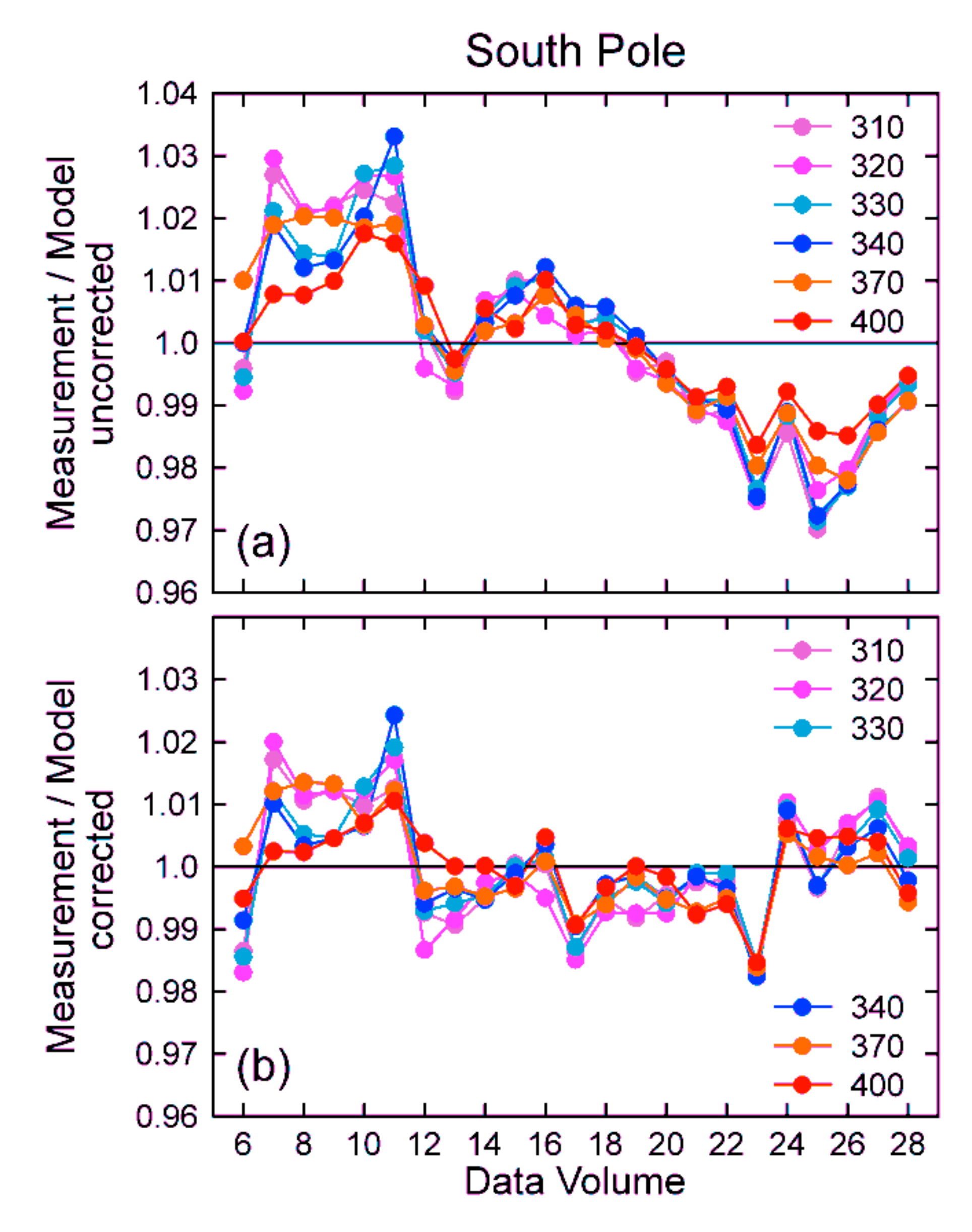
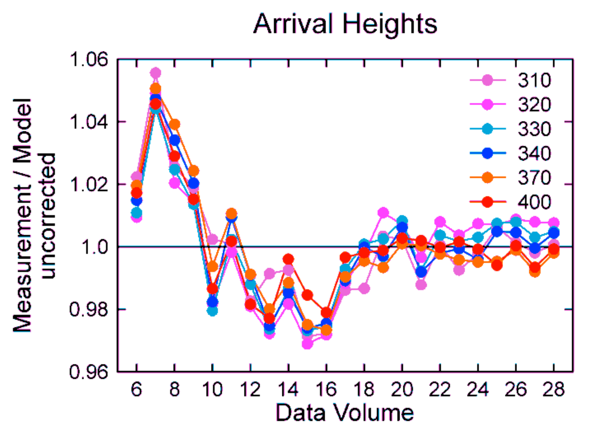
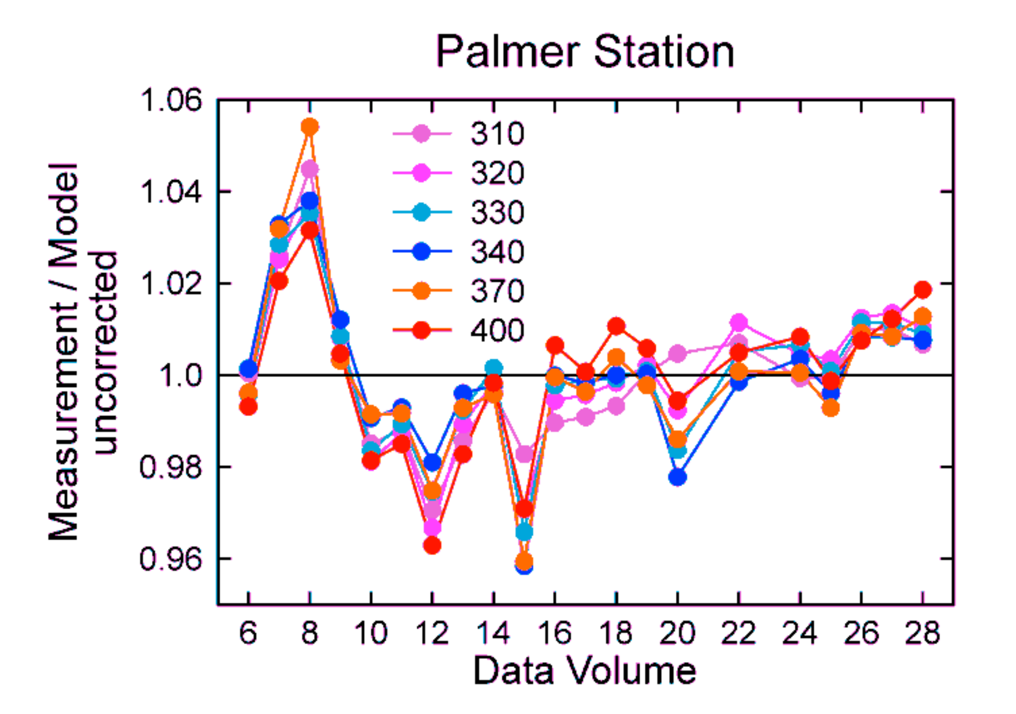
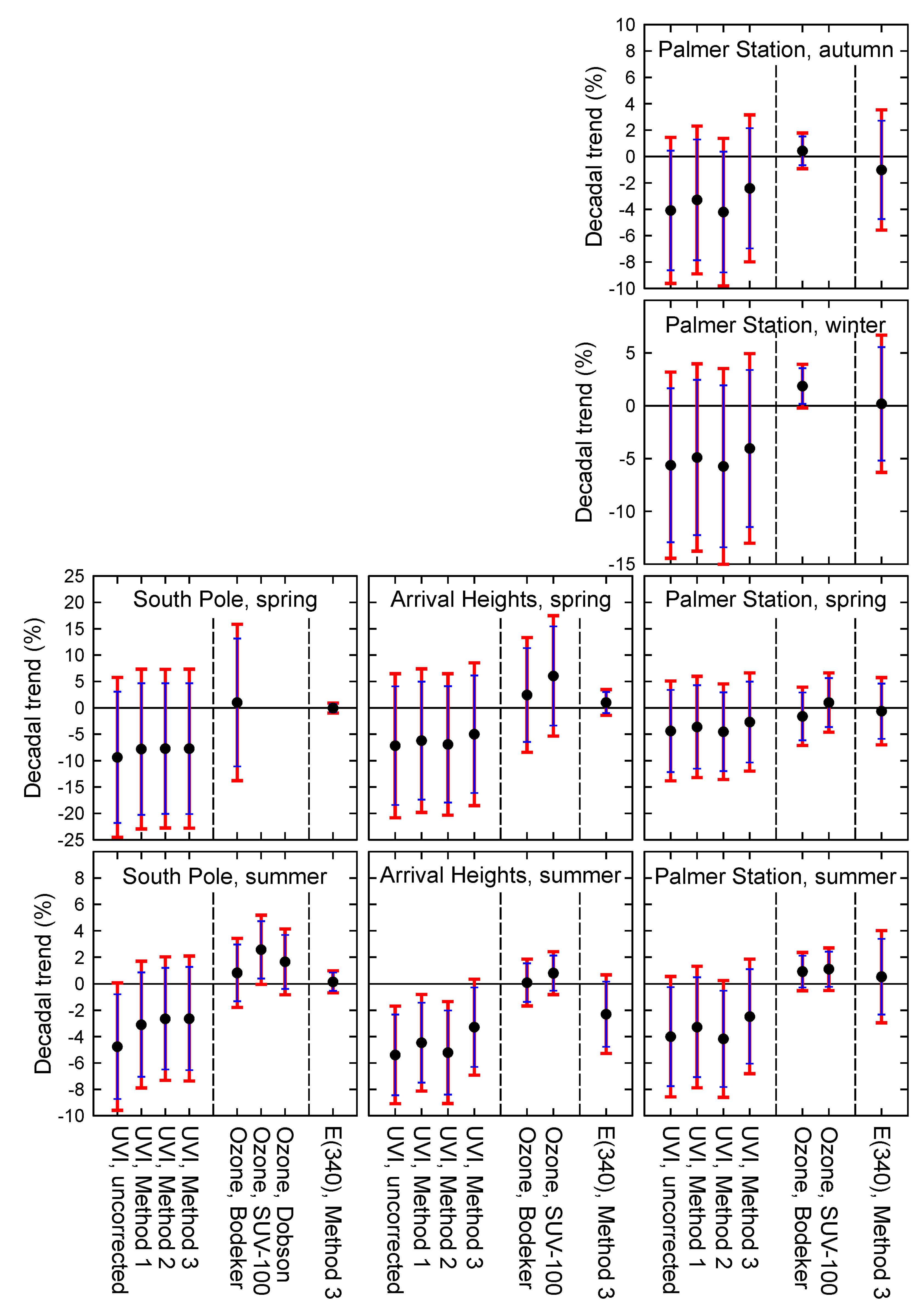
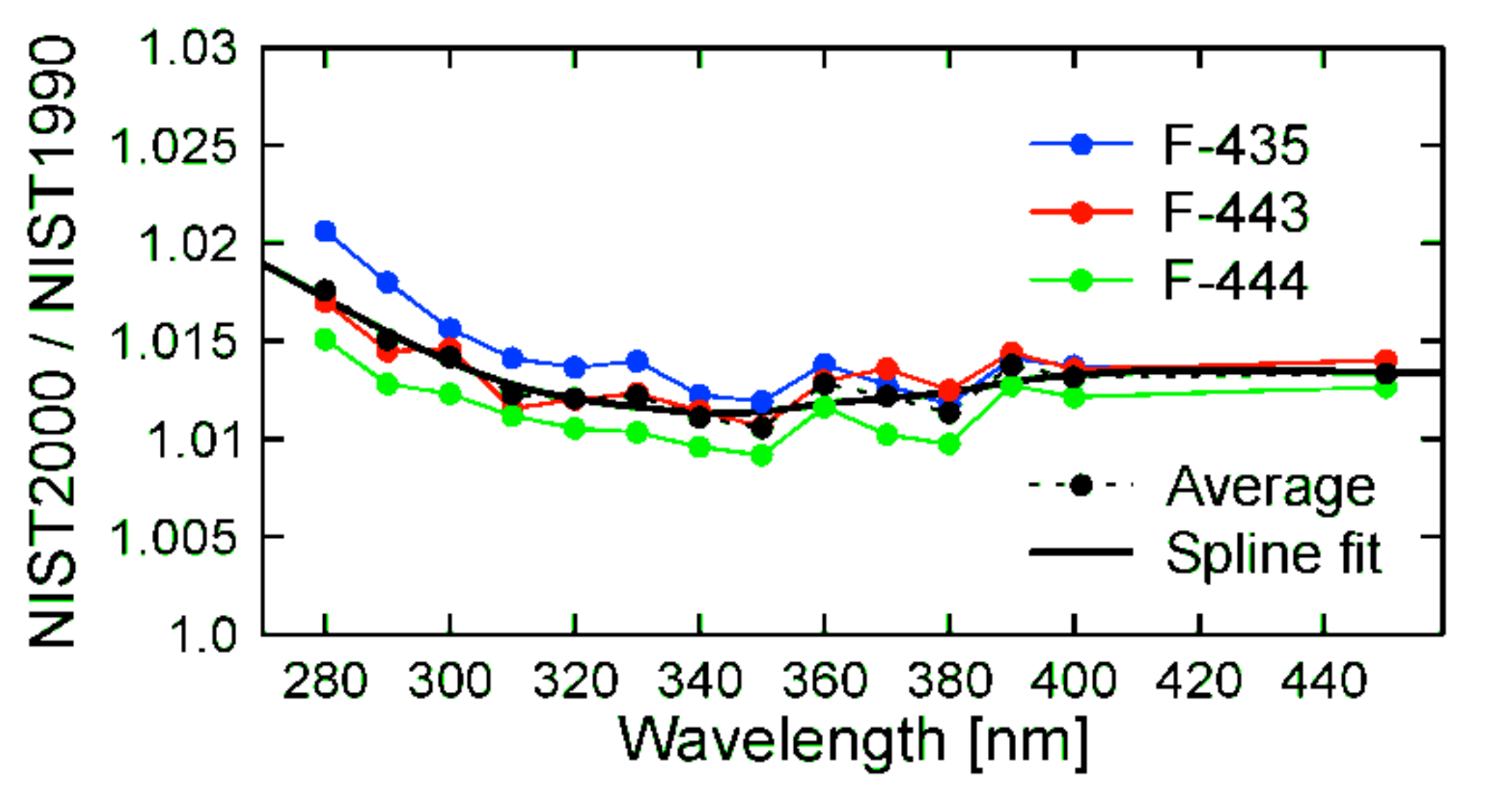
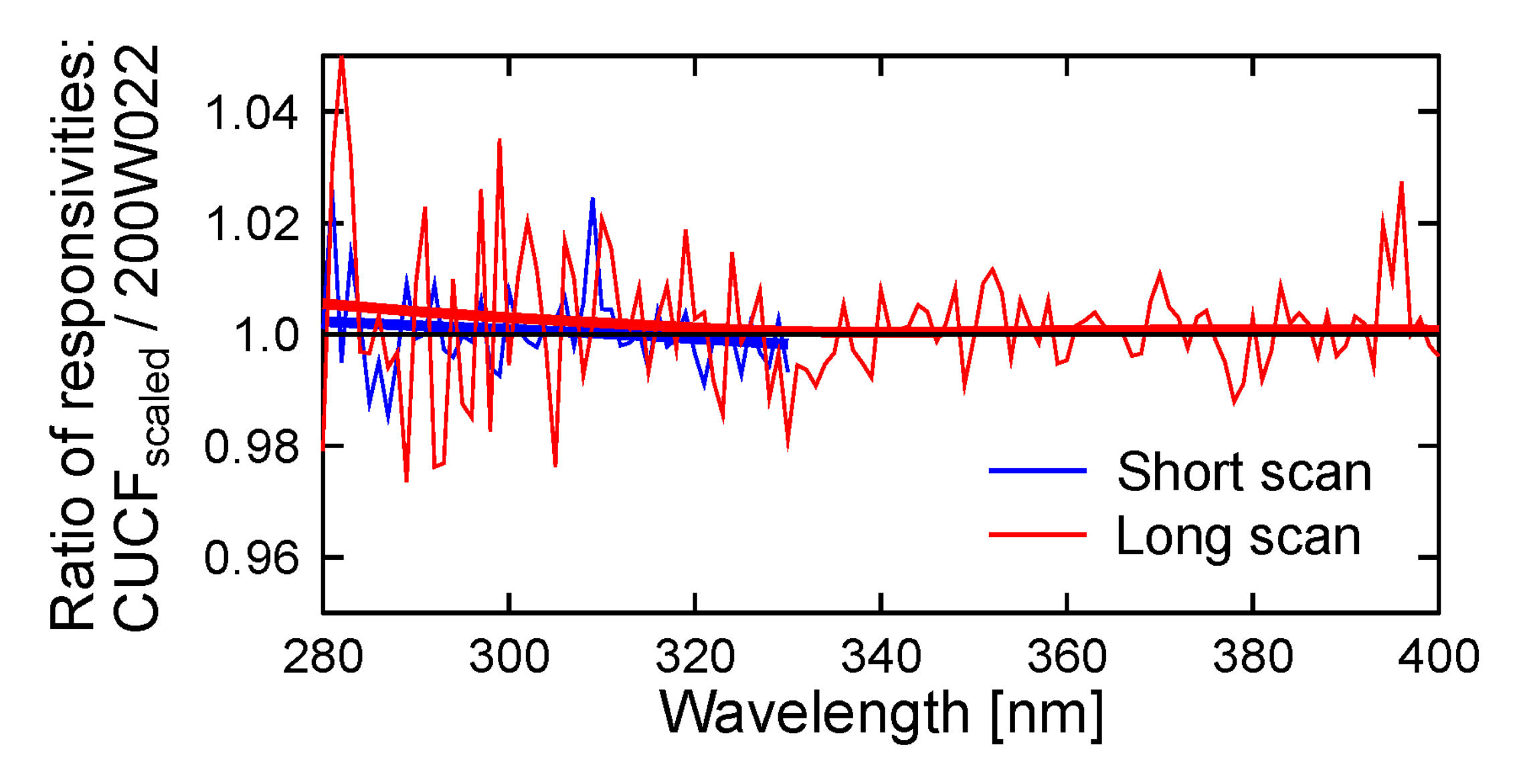
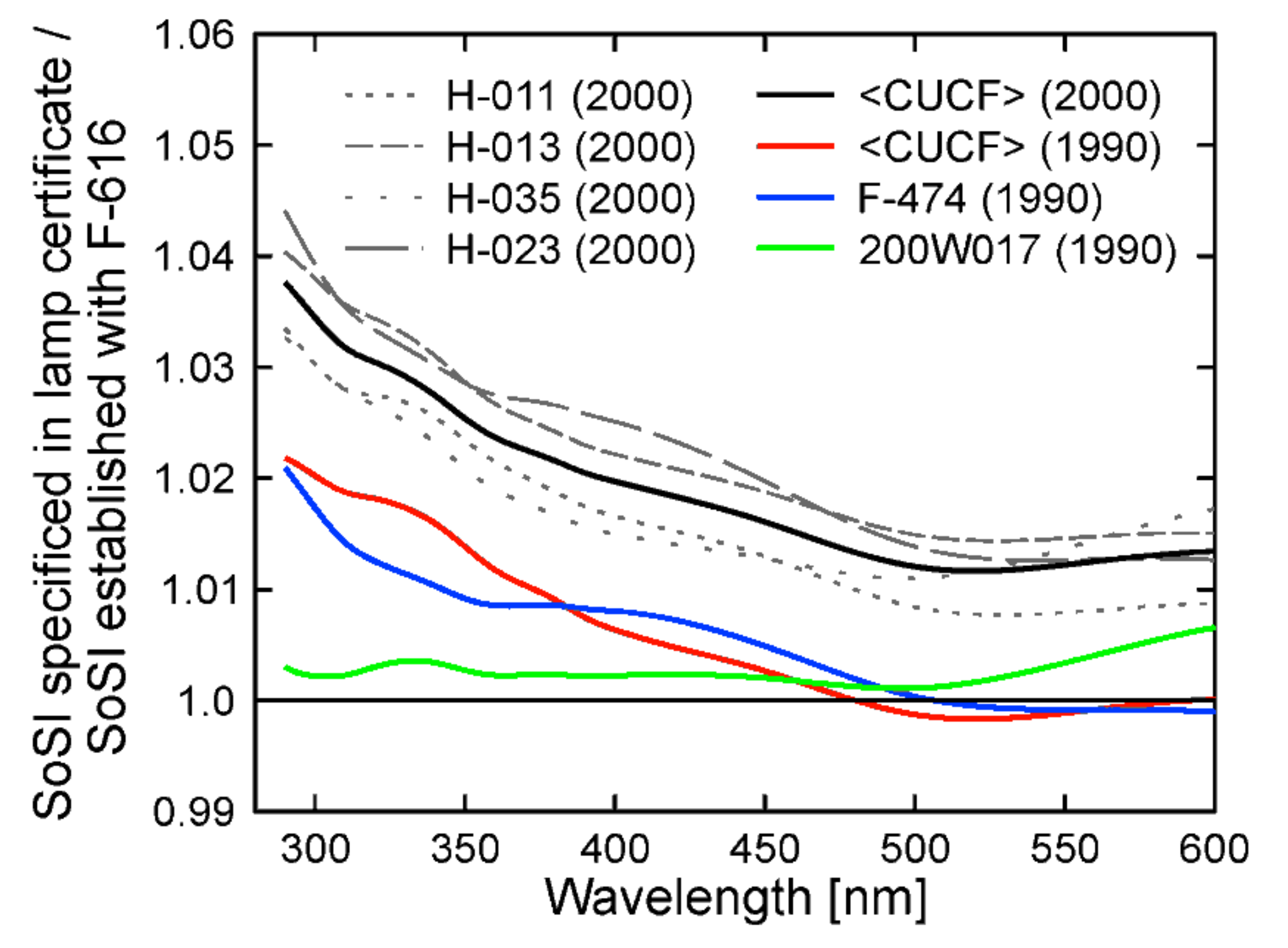
Table 1.
Assignment of data volumes (Volume) to observation periods (Period, indicated by month/year start and end); traceability of the scales of spectral irradiance (SoSI); and correction factors derived either with Method 1 (review of SoSI (Section 2.4 and Section 2.5)); Method 2 (comparison with model spectra (Section 2.6)); or with a combination of both methods (Method 3, Section 2.7) for the South Pole, Arrival Heights, and Palmer Station. Values printed in bold face are affected by the change in the SoSI from the Central UV Calibration Facility (CUCF) standards to lamp F-616.
| Volume | South Pole | Arrival Heights | Palmer Station | ||||||||||||
|---|---|---|---|---|---|---|---|---|---|---|---|---|---|---|---|
| Period | Traceability | Method | Period | Traceability | Method | Period | Traceability | Method | |||||||
| SoSI | 1 | 2 | 3 | SoSI | 1 | 2 | 3 | SoSI | 1 | 2 | 3 | ||||
| 6 | 1/96–1/97 | OL | 1 | 1.008 | 1.016 | 1/96–1/97 | OL | 1 | 0.991 | 0.986 | 1/96–4/97 | OL | 1 | 1.004 | 1.000 |
| 7 | 1/97–1/98 | OL | 1 | 0.971 | 0.979 | 1/97–1/98 | OL | 1 | 0.953 | 0.949 | 4/97–3/98 | OL | 1 | 0.975 | 0.972 |
| 8 | 1/98–1/99 | OL | 1 | 0.979 | 0.987 | 1/98–1/99 | OL | 1 | 0.980 | 0.975 | 4/98–5/99 | OL | 1 | 0.964 | 0.960 |
| 9 | 1/99–1/00 | OL | 1 | 0.979 | 0.987 | 1/99–1/00 | OL | 1 | 0.986 | 0.981 | 5/99–3/00 | OL | 1 | 0.992 | 0.988 |
| 10 | 1/00–1/01 | OL | 0.995 | 0.974 | 0.995 | 2/00–1/01 | OL | 1 | 1.018 | 1 | 3/00–5/01 | OL | 1 | 1.019 | 1 |
| 11 | 1/01–1/02 | OL | 1 | 0.974 | 1 | 1/01–1/02 | OL | 1 | 1.002 | 1 | 7/01–7/02 | OL | 1 | 1.013 | 1 |
| 12 | 1/02–1/03 | OL | 1 | 1.004 | 1 | 1/02–1/03 | OL | 1 | 1.019 | 1 | 7/02–3/03 | OL | 1 | 1.034 | 1 |
| 13 | 1/03–1/04 | OL | 1.008 | 1.007 | 1.008 | 1/03–2/04 | OL | 1 | 1.029 | 1 | 3/03–5/04 | OL | 1 | 1.011 | 1 |
| 14 | 1/04–1/05 | OL | 1 | 0.993 | 1 | 2/04–1/05 | OL | 1 | 1.019 | 1 | 6/04–6/05 | OL | 1 | 1.002 | 1 |
| 15 | 1/05–1/06 | OL | 1 | 0.992 | 1 | 1/05–1/06 | OL | 1 | 1.032 | 1 | 6/05–4/06 | OL | 1 | 1.030 | 1 |
| 16 | 1/06–1/07 | OL | 1 | 0.996 | 1 | 1/06–1/07 | OL | 1 | 1.029 | 1 | 4/06–7/07 | OL | 1 | 1.006 | 1 |
| 17 | 1/07–1/08 | OL/CUCF | 0.993 | 0.999 | 0.993 | 1/07–1/08 | CUCF | 1 | 1.012 | 1 | 7/07–5/08 | OL/CUCF | 1 | 1.004 | 1 |
| 18 | 1/08–3/09 | CUCF | 1 | 0.998 | 1 | 2/08–3/09 | CUCF | 1.008 | 1.002 | 1.008 | 5/08–2/09 | OL/CUCF | 1 | 1.002 | 1 |
| 19 | 9/09–3/10 | CUCF | 1.006 | 1.004 | 1.006 | 4/09–2/10 | CUCF | 1.019 | 0.989 | 1.019 | 3/09–9/10 | CUCF | 1 | 0.998 | 1 |
| 20 | 9/10–3/11 | CUCF | 1.008 | 1.006 | 1.008 | 8/10–4/11 | CUCF | 1 | 0.993 | 1 | 10/10–12/11 | CUCF | 1 | 1.008 | 1 |
| 21 | 9/11–3/12 | CUCF/F-616 | 1.017 | 1.011 | 1.017 | 8/11–4/12 | CUCF | 1 | 1.003 | 1 | – | – | – | – | – |
| 22 | 9/12–3/13 | CUCF/F-616 | 1.017 | 1.013 | 1.017 | 8/12–4/13 | F-616 | 1.0175 | 0.992 | 1.0175 | 1/12–12/13 | CUCF | 1 | 0.989 | 1 |
| 23 | 9/13–3/14 | CUCF/F-616 | 1.017 | 1.026 | 1.017 | 8/13–4/14 | F-616 | 1.0175 | 0.996 | 1.0175 | – | – | – | – | – |
| 24 | 9/14–3/15 | F-616 | 1.030 | 1.011 | 1.030 | 8/14–4/15 | F-616 | 1.0175 | 0.993 | 1.0175 | 1/14–3/15 | F-616 | 1.018 | 0.995 | 1.018 |
| 25 | 9/15–3/16 | F-616 | 1.035 | 1.024 | 1.035 | 8/15–4/16 | F-616 | 1.0175 | 0.993 | 1.0175 | 3/15–7/16 | F-616 | 1.018 | 0.997 | 1.018 |
| 26 | 9/16–3/17 | F-616 | 1.036 | 1.021 | 1.036 | 8/16–4/17 | F-616 | 1.0175 | 0.991 | 1.0175 | 8/16–5/17 | F-616 | 1.018 | 0.988 | 1.018 |
| 27 | 9/17–3/18 | F-616 | 1.030 | 1.011 | 1.030 | 8/17–4/18 | F-616 | 1.0175 | 0.992 | 1.0175 | 6/17–6/18 | F-616 | 1.018 | 0.987 | 1.018 |
| 28 | 9/18–3/19 | F-616 | 1.017 | 1.005 | 1.017 | 8/18–4/19 | F-616 | 1.0175 | 0.992 | 1.0175 | 7/18–3/19 | F-616 | 1.018 | 0.990 | 1.018 |
Table 2.
Trends in UVI, TOC, and E(340) at the South Pole and Arrival Heights in percent per decade. The first value after “±” indicates the uncertainty at the 95% level of confidence. The value in parenthesis is the uncertainty at the 90% level. Trends that are statistically significant at the 95% level are indicated in bold face. For trends that are significant at the 90% level, only the uncertainty provided in parenthesis is printed in bold face.
| Period | Trend (% per Decade) | |||||||
|---|---|---|---|---|---|---|---|---|
| Uvi | Total Ozone Column | E (340) | ||||||
| Uncorrected | Corrected with | Bodeker | SUV-100 | Dobson | Corrected with | |||
| Method 1 | Method 2 | Method 3 | Method 3 | |||||
| South Pole | ||||||||
| Jan | −5.5 ± 2.0 (±1.6) | −4.1 ± 2.0 (±1.7) | −3.9 ± 1.7 (±1.4) | −3.9 ± 1.9 (±1.5) | 1.8 ± 1.9 (±1.6) | 3.1 ± 1.5 (±1.2) | 2.8 ± 1.6 (±1.3) | −0.3 ± 0.9 (±0.7) |
| Feb | −4.7 ± 2.9 (±2.4) | −3.2 ± 3.0 (±2.5) | −3.1 ± 2.8 (±2.3) | −3.1 ± 3.0 (±2.5) | 1.1 ± 3.1 (±2.6) | 2.4 ± 2.8 (±2.3) | 1.2 ± 3.0 (±2.5) | −0.3 ± 0.8 (±0.6) |
| Mar | −2.5 ± 3.6 (±2.9) | −0.9 ± 3.6 (±3.0) | −0.6 ± 3.6 (±2.9) | −0.6 ± 3.7 (±3.0) | −1.8 ± 2.5 (±2.0) | −1.1 ± 1.4 (±1.2) | ||
| Oct | −5.0 ± 12.2 (±10.1) | −3.3 ± 12.3 (±10.2) | −3.3 ± 12.1 (±10.0) | −3.2 ± 12.3 (±10.1) | −1.5 ± 12.6 (±10.3) | 4.4 ± 11.6 (±9.5) | 0.3 ± 1.3 (±1.1) | |
| Nov | −9.7 ± 16.0 (±13.1) | −8.2 ± 15.9 (±13.0) | −7.9 ± 15.9 (±13.0) | −8.0 ± 15.9 (±13.0) | 4.4 ± 16.8 (±13.7) | 6.5 ± 16.4 (±13.4) | 7.4 ± 16.4 (±13.4) | −0.1 ± 0.8 (±0.7) |
| Dec | −2.5 ± 8.0 (±6.6) | −1.0 ± 8.0 (±6.5) | −0.7 ± 7.9 (±6.4) | −0.7 ± 7.9 (±6.5) | −0.6 ± 5.5 (±4.5) | 1.2 ± 5.6 (±4.6) | 1.0 ± 5.5 (±4.5) | 0.8 ± 1.1 (±0.9) |
| Dec–Feb | −4.8 ± 4.8 (±4.0) | −3.1 ± 4.8 (±3.9) | −2.6 ± 4.7 (±3.8) | −2.6 ± 4.7 (±3.9) | 0.8 ± 2.6 (±2.1) | 2.6 ± 2.6 (±2.2) | 1.7 ± 2.5 (±2.0) | 0.2 ± 0.8 (±0.7) |
| Sep–Nov | −9.4 ± 15.1 (±12.5) | −7.8 ± 15.1 (±12.5) | −7.7 ± 15.0 (±12.4) | −7.7 ± 15.1 (±12.4) | 1.0 ± 14.8 (±12.1) | 0.0 ± 0.9 (±0.8) | ||
| Arrival Heights | ||||||||
| Jan | −4.7 ± 3.7 (±3.1) | −3.8 ± 3.7 (±3.0) | −4.6 ± 3.7 (±3.1) | −2.6 ± 3.5 (±2.9) | 0.7 ± 1.5 (±1.2) | 1.5 ± 1.6 (±1.3) | −0.7 ± 3.6 (±3.0) | |
| Feb | −7.1 ± 6.8 (±5.6) | −6.3 ± 6.7 (±5.6) | −7.2 ± 7.5 (±6.2) | −5.3 ± 7.1 (±5.8) | −0.1 ± 2.4 (±2.0) | −0.1 ± 2.2 (±1.9) | −4.7 ± 5.8 (±4.8) | |
| Mar | −6.4 ± 7.3 (±6.0) | −5.5 ± 7.2 (±5.9) | −6.5 ± 8.1 (±6.7) | −4.6 ± 7.5 (±6.2) | 0.3 ± 2.5 (±2.0) | 1.0 ± 2.2 (±1.8) | −3.8 ± 6.8 (±5.6) | |
| Apr | −3.2 ± 7.6 (±6.2) | −2.2 ± 7.5 (±6.2) | −3.3 ± 8.0 (±6.6) | −1.2 ± 7.6 (±6.3) | −0.1 ± 2.1 (±1.7) | −0.7 ± 6.1 (±5.0) | ||
| Sep | −8.5 ± 11.4 (±9.4) | −7.5 ± 11.5 (±9.5) | −8.3 ± 11.3 (±9.3) | −6.3 ± 11.5 (±9.5) | 2.1 ± 10.0 (±8.2) | 4.2 ± 11.4 (±9.4) | 0.2 ± 3.5 (±2.9) | |
| Oct | −10.6 ± 15.8 (±13.0) | −9.7 ± 15.7 (±12.9) | −10.3 ± 15.4 (±12.7) | −8.4 ± 15.5 (±12.8) | 2.9 ± 14.4 (±11.8) | 9.3 ± 13.9 (±11.4) | 0.1 ± 2.8 (±2.3) | |
| Nov | −5.1 ± 15.3 (±12.6) | −4.2 ± 15.3 (±12.6) | −4.9 ± 15.2 (±12.5) | −3.0 ± 15.3 (±12.6) | 2.3 ± 12.4 (±10.1) | 4.6 ± 12.7 (±10.5) | 1.8 ± 2.7 (±2.2) | |
| Dec | −5.5 ± 5.5 (±4.5) | −4.5 ± 5.4 (±4.5) | −5.3 ± 5.6 (±4.6) | −3.4 ± 5.4 (±4.4) | −0.2 ± 3.9 (±3.2) | 1.3 ± 4.1 (±3.4) | −1.5 ± 2.9 (±2.4) | |
| Dec–Feb | −5.4 ± 3.7 (±3.1) | −4.5 ± 3.7 (±3.0) | −5.2 ± 3.9 (±3.2) | −3.3 ± 3.6 (±3.0) | 0.1 ± 1.8 (±1.5) | 0.8 ± 1.6 (±1.3) | −2.3 ± 3.0 (±2.5) | |
| Sep–Nov | −7.2 ± 13.7 (±11.2) | −6.2 ± 13.6 (±11.2) | −6.9 ± 13.4 (±11.0) | −5.0 ± 13.5 (±11.1) | 2.4 ± 10.9 (±8.9) | 6.1 ± 11.4 (±9.4) | 1.0 ± 2.4 (±2.0) | |
Table 3.
Same as Table 2 but for Palmer Station.
Table 3.
Same as Table 2 but for Palmer Station.
| Period | Trend (% per Decade) | ||||||
|---|---|---|---|---|---|---|---|
| UVI | Total Ozone Column | E (340) | |||||
| Uncorrected | Corrected with | Bodeker | SUV–100 | Corrected with | |||
| Method 1 | Method 2 | Method 3 | Method 3 | ||||
| Palmer Station | |||||||
| Jan | –4.0 ± 4.4 (±3.6) | –3.3 ± 4.4 (±3.6) | –4.4 ± 4.7 (±3.8) | –2.6 ± 4.3 (±3.5) | –0.2 ± 2.1 (±1.7) | 0.0 ± 2.4 (±1.9) | –1.9 ± 4.1 (±3.3) |
| Feb | –0.3 ± 6.1 (±5.0) | 0.5 ± 6.0 (±4.9) | –0.6 ± 5.9 (±4.8) | 1.2 ± 5.9 (±4.8) | 0.5 ± 2.2 (±1.8) | 0.6 ± 2.4 (±2.0) | 3.4 ± 5.5 (±4.5) |
| Mar | –5.4 ± 6.7 (±5.5) | –4.6 ± 6.7 (±5.5) | –5.7 ± 6.5 (±5.3) | –3.9 ± 6.6 (±5.4) | 0.5 ± 1.9 (±1.6) | 0.7 ± 2.0 (±1.6) | –2.6 ± 5.7 (±4.7) |
| Apr | –0.4 ± 4.8 (±4.0) | 0.4 ± 4.9 (±4.1) | –0.5 ± 5.0 (±4.1) | 1.3 ± 5.0 (±4.1) | 0.6 ± 2.0 (±1.6) | –0.9 ± 2.3 (±1.9) | 2.3 ± 3.9 (±3.2) |
| May | –3.1 ± 4.4 (±3.6) | –2.3 ± 4.4 (±3.7) | –2.9 ± 4.6 (±3.8) | –1.2 ± 4.5 (±3.7) | 0.1 ± 2.2 (±1.8) | –1.9 ± 3.6 (±3.0) | |
| Jun | –8.9 ± 4.7 (±3.9) | –8.1 ± 4.8 (±3.9) | –8.9 ± 4.9 (±4.1) | –7.3 ± 4.8 (±4.0) | 1.9 ± 1.8 (±1.5) | –4.6 ± 4.0 (±3.3) | |
| Jul | 1.2 ± 8.9 (±7.3) | 1.9 ± 9.0 (±7.5) | 1.0 ± 9.2 (±7.7) | 2.8 ± 9.0 (±7.4) | 0.9 ± 2.8 (±2.3) | 3.8 ± 7.7 (±6.4) | |
| Aug | –6.7 ± 9.5 (±7.9) | –6.0 ± 9.6 (±7.9) | –7.0 ± 10.1 (±8.3) | –5.2 ± 9.7 (±8.0) | 3.0 ± 3.5 (±2.8) | 5.0 ± 4.0 (±3.3) | –0.3 ± 7.0 (±5.8) |
| Sep | –7.1 ± 13.4 (±11.0) | –6.4 ± 13.4 (±11.1) | –7.4 ± 13.6 (±11.2) | –5.5 ± 13.4 (±11.0) | 0.6 ± 7.6 (±6.2) | 4.7 ± 7.9 (±6.5) | –1.2 ± 8.7 (±7.2) |
| Oct | –5.7 ± 12.5 (±10.3) | –5.0 ± 12.5 (±10.3) | –5.9 ± 12.3 (±10.1) | –4.0 ± 12.3 (±10.1) | –2.0 ± 9.0 (±7.3) | 1.5 ± 8.2 (±6.8) | 0.7 ± 7.4 (±6.1) |
| Nov | –2.3 ± 15.0 (±12.4) | –1.6 ± 15.1 (±12.5) | –2.4 ± 14.6 (±12.0) | –0.6 ± 14.9 (±12.3) | –2.9 ± 9.8 (±8.0) | –2.1 ± 10.8 (±8.8) | –1.4 ± 7.2 (±5.9) |
| Dec | –4.8 ± 7.9 (±6.5) | –4.1 ± 8.0 (±6.5) | –5.0 ± 7.4 (±6.1) | –3.2 ± 7.6 (±6.3) | 2.2 ± 2.5 (±2.1) | 1.8 ± 2.7 (±2.3) | 1.9 ± 6.2 (±5.1) |
| Dec–Feb | –4.0 ± 4.6 (±3.8) | –3.3 ± 4.6 (±3.8) | –4.2 ± 4.4 (±3.6) | –2.5 ± 4.3 (±3.6) | 0.9 ± 1.4 (±1.2) | 1.1 ± 1.6 (±1.3) | 0.5 ± 3.5 (±2.9) |
| Mar–May | –4.1 ± 5.5 (±4.5) | –3.3 ± 5.6 (±4.6) | –4.2 ± 5.6 (±4.6) | –2.4 ± 5.6 (±4.6) | 0.4 ± 1.3 (±1.1) | –1.0 ± 4.6 (±3.7) | |
| Jun–Aug | –5.6 ± 8.8 (±7.3) | –4.9 ± 8.9 (±7.4) | –5.7 ± 9.3 (±7.7) | –4.0 ± 9.0 (±7.4) | 1.9 ± 2.1 (±1.7) | 0.2 ± 6.5 (±5.4) | |
| Sep–Nov | –4.4 ± 9.5 (±7.8) | –3.6 ± 9.6 (±7.9) | –4.5 ± 9.1 (±7.5) | –2.7 ± 9.3 (±7.7) | –1.6 ± 5.5 (±4.5) | 1.0 ± 5.6 (±4.6) | –0.6 ± 6.4 (±5.2) |
Table 4.
Trends in UVI, TOC, and E(340) at the South Pole calculated either for the period January 1996–March 2019 (columns “Mar 2019”) as in the work by McKenzie et al. [14] or for the period January 1996–March 2020 (columns “Mar 2020”), which includes the period of the small ozone hole in the spring of 2019. UVI and E(340) trends were corrected with Method 3. Uncertainties of trends are provided at the 95% level. Trends that are statistically significant are indicated in bold face.
| Period | Trend at South Pole (% per Decade) | |||||||||
|---|---|---|---|---|---|---|---|---|---|---|
| UVI | Total Ozone Column | E (340) | ||||||||
| SUV-100 | Dobson | |||||||||
| Mar 2019 | Mar 2020 | Mar 2019 | Mar 2020 | Mar 2019 | Mar 2020 | Mar 2019 | Mar 2020 | |||
| Jan | −3.9 ± 1.9 | −4.2 ± 1.7 | 3.1 ± 1.5 | 3.4 ± 1.4 | 2.8 ± 1.6 | 3.0 ± 1.5 | −0.3 ± 0.9 | −0.3 ± 0.8 | ||
| Feb | −3.1 ± 3.0 | −3.2 ± 2.8 | 2.4 ± 2.8 | 2.6 ± 2.6 | 1.2 ± 3.0 | 1.7 ± 2.8 | −0.3 ± 0.8 | −0.5 ± 0.7 | ||
| Mar | −0.6 ± 3.7 | −1.3 ± 3.5 | −1.1 ± 1.4 | −1.5 ± 1.4 | ||||||
| Oct | −3.2 ± 12.3 | −6.7 ± 12.1 | 4.4 ± 11.6 | 8.8 ± 11.7 | 8.0 ± 14.5 | 13.0 ± 14.6 | 0.3 ± 1.3 | 0.1 ± 1.2 | ||
| Nov | −8.0 ± 15.9 | −10.9 ± 15.1 | 6.5 ± 16.4 | 10.3 ± 15.5 | 7.4 ± 16.4 | 10.8 ± 15.4 | −0.1 ± 0.8 | −0.2 ± 0.8 | ||
| Dec | −0.7 ± 7.9 | −2.1 ± 7.4 | 1.2 ± 5.6 | 2.2 ± 5.3 | 1.0 ± 5.5 | 2.0 ± 5.2 | 0.8 ± 1.1 | 0.7 ± 1.0 | ||
| Dec−Feb | −2.6 ± 4.7 | −3.1 ± 4.0 | 2.6 ± 2.6 | 2.8 ± 2.3 | 1.7 ± 2.5 | 2.0 ± 2.2 | 0.2 ± 0.8 | −0.1 ± 0.7 | ||
| Sep−Nov | −7.7 ± 15.1 | −10.8 ± 14.4 | 0.0 ± 0.9 | −0.2 ± 0.9 | ||||||
Table 5.
Trends in UVI, TOC, and E(340) at Arrival Heights calculated either for the period January 1996–April 2018 (columns “Apr 2018”) as in the work by McKenzie et al. [14] or for the period January 1996–April 2020 (columns “Apr 2020”), which includes the period of the small ozone hole in the spring of 2019. UVI and E(340) trends were corrected with Method 3. Uncertainties of trends are provided at the 95% level. Trends that are statistically significant are indicated in bold face.
| Period | Trend at Arrival Heights (% per Decade) | |||||
|---|---|---|---|---|---|---|
| UVI | Total Ozone Column SUV-100 | E (340) | ||||
| April 2018 | April 2020 | April 2018 | April 2020 | April 2018 | April 2020 | |
| Jan | −2.6 ± 3.5 | −2.3 ± 3.0 | 1.5 ± 1.6 | 2.1 ± 1.4 | −0.7 ± 3.6 | 0.0 ± 3.1 |
| Feb | −5.3 ± 7.1 | −7.3 ± 6.2 | −0.1 ± 2.2 | 0.7 ± 2.0 | −4.7 ± 5.8 | −6.3 ± 5.0 |
| Mar | −4.6 ± 7.5 | −6.4 ± 6.5 | 1.0 ± 2.2 | 1.2 ± 1.9 | −3.8 ± 6.8 | −5.2 ± 5.9 |
| Apr | −1.2 ± 7.6 | −2.5 ± 6.6 | −0.7 ± 6.1 | −1.8 ± 5.4 | ||
| Sep | −6.3 ± 11.5 | −9.6 ± 10.9 | 4.2 ± 11.4 | 9.5 ± 13.2 | 0.2 ± 3.5 | −0.6 ± 3.0 |
| Oct | −8.4 ± 15.5 | −8.7 ± 14.1 | 9.3 ± 13.9 | 10.1 ± 13.3 | 0.1 ± 2.8 | −0.6 ± 2.5 |
| Nov | −3.0 ± 15.3 | −5.4 ± 13.3 | 4.6 ± 12.7 | 6.1 ± 11.0 | 1.8 ± 2.7 | 1.1 ± 2.4 |
| Dec | −3.4 ± 5.4 | −3.1 ± 4.5 | 1.3 ± 4.1 | 1.6 ± 3.5 | −1.5 ± 2.9 | −1.0 ± 2.4 |
| Dec−Feb | −3.3 ± 3.6 | −3.0 ± 2.8 | 0.8 ± 1.6 | 1.2 ± 1.4 | −2.3 ± 3.0 | −1.8 ± 2.3 |
| Sep−Nov | −5.0 ± 13.5 | −6.8 ± 12.1 | 6.1 ± 11.4 | 8.2 ± 11.0 | 1.0 ± 2.4 | −0.3 ± 2.0 |
© 2020 by the authors. Licensee MDPI, Basel, Switzerland. This article is an open access article distributed under the terms and conditions of the Creative Commons Attribution (CC BY) license (http://creativecommons.org/licenses/by/4.0/).
Share and Cite
MDPI and ACS Style
Bernhard, G.; Stierle, S. Trends of UV Radiation in Antarctica. Atmosphere 2020, 11, 795. https://doi.org/10.3390/atmos11080795
AMA Style
Bernhard G, Stierle S. Trends of UV Radiation in Antarctica. Atmosphere. 2020; 11(8):795. https://doi.org/10.3390/atmos11080795
Chicago/Turabian StyleBernhard, Germar, and Scott Stierle. 2020. "Trends of UV Radiation in Antarctica" Atmosphere 11, no. 8: 795. https://doi.org/10.3390/atmos11080795
Note that from the first issue of 2016, this journal uses article numbers instead of page numbers. See further details here.