Article

Hourly Elemental Composition and Source Identification by Positive Matrix Factorization (PMF) of Fine and Coarse Particulate Matter in the High Polluted Industrial Area of Taranto (Italy)

Department of Physics and Astronomy, University of Florence and National Institute of Nuclear Physics (INFN), Via Sansone 1, 50019 Sesto Fiorentino (FI), Italy
*
Author to whom correspondence should be addressed.
Atmosphere 2020, 11(4), 419; https://doi.org/10.3390/atmos11040419
Submission received: 23 March 2020 / Revised: 15 April 2020 / Accepted: 17 April 2020 / Published: 21 April 2020
(This article belongs to the Special Issue Recent Advances of Air Pollution Studies in Italy)

Abstract

:
In the framework of an extensive environmental investigation, promoted by the Italian Health Ministry, the ISPESL (Istituto Superiore per la Prevenzione e la Sicurezza del Lavoro) and the CNR (Consiglio Nazionale della Ricerca), aerosol samples were collected in Taranto (one of the most industrialized towns in southern Italy) with high time resolution and analyzed by PIXE. The samples were collected in two periods (February–March and June 2004) and in two different sites: an urban district close to the industrial area and a small town 7 km N-NW of Taranto. The use of ‘‘streaker’’ samplers (by PIXE International Corporation) allowed for the simultaneous collection of the fine (<2.5 μm) and coarse (2.5–10 μm) fractions of particulate matter. PIXE analyses were performed with a 3 MeV proton beam from the 3 MV Tandetron accelerator of the INFN-LABEC laboratory. Particulate emissions as well as their atmospheric transport and dilution processes change within a few hours, but most of the results in literature are limited to daily time resolution of the input samples that are not suitable for tracking these rapid changes. Furthermore, since source apportionment receptor models need a series of samples containing material from the same set of sources in different proportions, a higher variability between samples can be obtained by increasing the temporal resolution rather than with samples integrated over a longer time. In this study, the high time resolution of the adopted approach allowed us to follow in detail the changes in the aerosol elemental composition due to both the time evolution of the industrial emissions and the time changes in meteorological conditions, and thus, transport pathways. Moreover, the location of the sampling sites, along the prevalent wind direction and in opposite positions with respect to the industrial site, allowed us to follow the impact of the industrial plume as a function of wind direction. Positive matrix factorization (PMF) analysis on the elemental hourly concentrations identified eight sources in the fine fraction and six sources in the coarse one.

1. Introduction

Taranto, an ancient Italian town with a population of around 196,000 people, is one of the most industrialized towns in the South of Italy. The city is known as the “city of two seas” because it is surrounded by the Great Sea and by the Little Sea. It has an important harbor, located near the city center, which is an important commercial port as well as the main Italian naval base with military and civil shipyards, contributing to the primary industrial activity. Besides being an important commercial and military port, Taranto has an extended industrial pole in the northern suburbs of the town, which includes one of the biggest Italian refineries, a power plant, a big cement industry and the biggest steel plant in Europe. These activities, developed very close to residential areas, heavily stress the environment of the town.
The integrated iron and steelmaking process is complicated and it involves a number of linked processes, from the extraction of iron from its ores in the blast furnace (BF) to the subsequent refinement of the melted iron into liquid steel by the basic oxygen steelmaking (BOS) process. The integrated process also includes iron ore sintering and coke making facilities necessary to prepare agglomerated iron ores and coke respectively, for use in the BF load [1]. The ILVA (Società Industria Laminati Piani e Affini) steel plant in Taranto is the largest steelworks in Europe. It is equipped with five blast furnaces and produces more than 30 percent of Italy’s raw steel [2]. In 1990, the area including Taranto and its surroundings was declared a zone of ‘high risk of environmental crisis’ and, in 1998, an extended sanitation plan was approved. During the last years, pollution problems of this area have come under the spotlight and have become a very compelling issue for the policy makers. Cancer rates in Taranto were found to be over 30 percent higher than the national average, especially for lungs, kidneys and liver, as well as melanomas. According to an epidemiological study, in seven years, up to 11,550 deaths could be linked to noxious emissions from the ILVA plant. In the considered period, about 27,000 people required some form of medical assistance for ailments that investigators ascribed to the pollution caused by the plant. Moreover, children in the age group under 14 living in this area have been suffering from cancers of the lung, larynx and bladder, in addition to an increased incidence of leukemia and other serious illnesses [3]. More than once, a court ordered to close sections of the plant, arguing that it had violated environmental laws and was raising serious health concerns in the area. The government was forced to pass emergency decrees that would allow it to continue operating while cleaning up its act, saving 20,000 jobs nationwide; however, frequently, the plant was running at reduced capacity.
For all these reasons, in 2004, the Italian Health Ministry, the ISPESL (Istituto Superiore per la Prevenzione e la Sicurezza del Lavoro) and the CNR (Consiglio Nazionale della Ricerca) promoted an extensive environmental investigation in this area. The aim was to quantify the pollution levels in air, soil and water and to identify their sources. Instrumentation by ISPESL and CNR was installed to analyze normal-alkanes, PAHs (polycyclic aromatic hydrocarbons), nitro-PAHs, organic acids, VOCs (volatile organic compounds), dioxins and PCBs (polychlorinated biphenyls).
Within this framework, we studied the aerosol composition with high time resolution (1 h). In the literature, most of the aerosol source apportionment studies use a limited time resolution, typically filter exposed for 12–24 h [4] to be analyzed off-line. This is due to several reasons such as the air flow rate of the sampler, the detection limit of the analytical method to be applied on the collected aerosol mass and the huge number of samples and data produced. However, better time resolution is necessary to catch the fast events typical of urban and industrialized environments, and to distinguish different aerosol sources. Due to the non-continuous nature of many steelmaking processes, traditional daily sampling with 24 h resolution does not have sufficient time resolution to capture short-time emission events arising from specific operations. A sampling with an hourly time basis better highlights the impact on PM levels and personal exposure of many sources, like industries or vehicular traffic, as an emission source. Furthermore, source apportionment receptor models need a series of samples containing material from the same set of sources in differing proportions. Hence, a high time resolution of the measurements is preferable to sample integrated over longer time periods, in order to have a greater inter-sample variability. Finally, the aim of this work was also to attribute emissions to specific production units in the integrated steel complex. To get representative source profiles is difficult; therefore, in the literature, the industrial emissions are the less documented among the primary anthropogenic emissions of aerosols. The number of industrial sources associated with a wide range of processes which are, in most cases, not continuous, accentuate this difficulty [5].

2. Experiments

Two sampling campaigns were performed in two different sites: Tamburi (site A) and Statte (site B). Site A is a densely populated urban district in Taranto adjacent to the industrial area which is subject to a heavy pollution flow. Site B is a small town located 7 km N-NW of Taranto and along the direction of prevalent winds from the industrial area (Figure 1). The location of the sampling sites was chosen in order to follow the impact of the industrial plume as a function of wind direction.
The sampling campaigns with streaker samplers (installed at about 4 m from the ground) were performed during winter (17 February 2004–16 March 2004) and summer (16–30 June 2004), simultaneously in A and B sites (see previous section). Both sampling periods were characterized by good and fairly stable weather conditions. Average values of temperature, pression, solar radiation, wind speed, dominant wind direction and precipitation were 11.3°, 1011 hPa, 118 W/m2, 5 m/s, SE-NW, 0.01 mm and 26.5°, 1014 hPa, 301 W/m2, 2.6 m/s, NE-SW, 0 mm respectively, in the winter and in the summer campaign. The sampling devices (PIXE International Corporation [6]) are designed to separate the fine (<2.5 µm aerodynamic diameter) and the coarse (2.5–10 µm) modes of atmospheric aerosol. Coarse particles are collected on an impaction surface made up of a paraffin-coated Kapton foil, whereas fine particles bypass this stage and end up on a Nuclepore filter. Both the collecting plates are paired on a cartridge, which rotates at constant speed for a week. This produces a circular continuous deposition of particulate matter on the two stages. The final resolution on the elemental composition of PM is one hour, thanks to the sampling rotation speed, the pumping orifice width and the beam size of the subsequent analysis. Three weeks, two during winter and one in summer, were selected for PIXE analysis among the sampled ones: February 23–March 8 and June 23–June 30. PIXE analyses were performed with 3 MeV protons from the 3 MV Tandetron accelerator of the LABEC laboratory of INFN in Florence, with the external beam set-up extensively described elsewhere [7,8]. The deposit streak was scanned in steps corresponding to 1 h of aerosol sampling. Each spot was irradiated using a 30–80 nA beam current for about 180 s. PIXE spectra were fitted using the GUPIX software package [9]. A set of thin standards of known areal density allowed for calculating the elemental concentrations of the following elements: Na, Mg, Al, P, S, Cl, K, Ca, Ti, V, Cr, Mn, Fe, Ni, Cu, Zn, Br, Sr and Pb. The uncertainties for each hourly elemental concentration value were determined by a sum of independent uncertainties on: standard samples thickness (5%), aerosol deposition area (2%), airflow (2%) and X-rays counting statistics (2–20%). The uncertainties are indeed higher for concentration values approaching the minimum detection limits (MDL). Detection limits were about 10 ng m−3 for low-Z elements and 1 ng m−3 (or below) for medium-high Z elements.
Finally, PMF (positive matrix factorization) analysis was carried out, for the identification of the aerosol sources. PMF is an advanced factor analysis procedure based on a weighted least square fit method [10]. It exploits realistic error estimates to weigh data values and imposes non-negativity constraints in the factor computational process. The equation X = G × F + E is the base for the PMF factor model, with, X which is the known n by m matrix of the m chemical species concentrations in n samples, G is an n by p matrix of the contribution to the samples of the p sources, F is a p by m matrix of factors composition (usually called source profiles) and E is the matrix of the residuals, which are the difference between the measured concentrations (X) and the values reconstructed from the model (G × F). The aim of the model is determining the G and F factor matrices that minimize the sum of the squares of the inversely weighed residuals with uncertainty estimates of the data points. Besides, the model constrains G and F to have non-negative elements, which means that sources cannot have negative species concentration (fkj ≥ 0) and samples cannot receive a negative source contribution (gik ≥ 0).
The source apportionment analysis was carried out by means of the PMF-EPA5 software package using only PIXE data as input. Indeed, important components including primary and secondary organic and inorganic species (organic carbon, elemental carbon, secondary inorganic ions, etc.) are not taken into account in the present study (because they were not available with the due temporal resolution at the time of the campaigns). Furthermore, direct information on the mass of streaker samples is not available so the results can be used for a detailed source identification but source time series will be expressed in arbitrary units [11].
Datasets from the two sites were analyzed together, as the sources affecting both sites are expected to be the same, while the two fractions were analyzed independently, as source profiles may vary depending on the PM fraction. The Polissar et al. [12] procedure was used to handle the data and their associated uncertainties as input for the PMF. PMF solutions ranging from 5 to 10 factors were systematically explored (also changing the FPEAK value) and the resulting Q values, the scaled residuals and the F and G matrices were examined to find the most reasonable solution.

3. Results

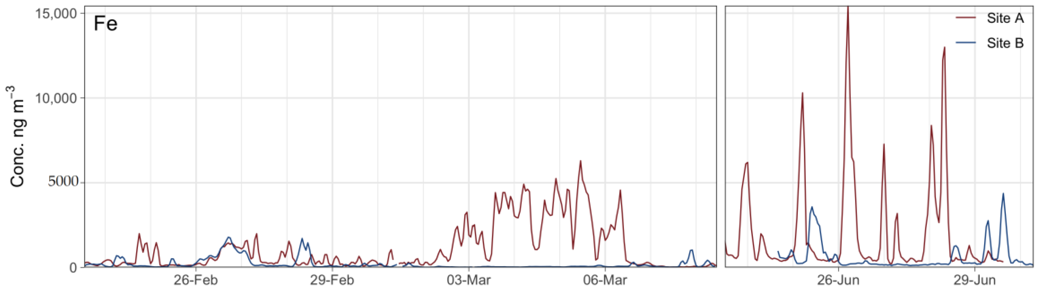
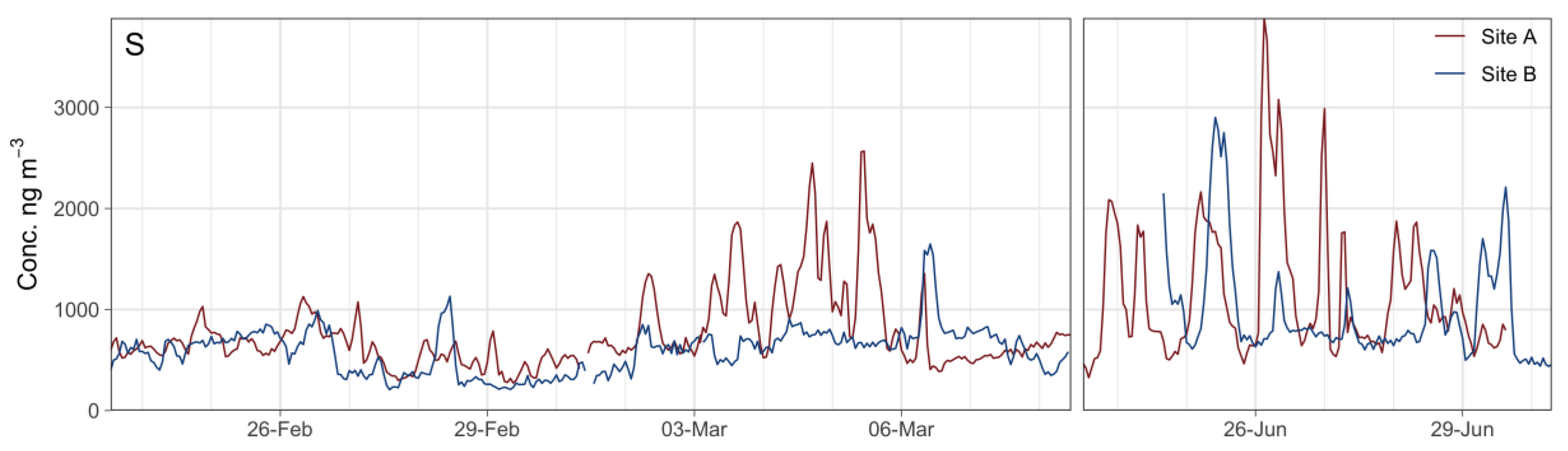
3.1. Elemental Mass Concentrations

An overview of the data on elemental concentrations measured at both sites in both fractions is reported as whisker plots in Figure 2. They range from values in the order of hundreds of ng/m3 (Al, Si, S, K, Ca and Fe in the fine fraction, Na, Mg, Al, Si, Cl, Ca and Fe in the coarse one) to tens of ng/m3 and below. Measurements in site A, which is closer to the industrial area, show higher concentrations for most of the elements, also considering PM10 (as the sum of the fine and coarse fraction). In particular, Ca, Fe, Cu and Zn are more than twice as much in site A with respect to site B. S, K, V, Cr, Ni, Cu, Zn and Pb are mainly present in the fine fraction, whereas Na, Mg, Cl and Ca are more abundant in the coarse one. Al, Si, Mn and Fe are quite balanced in the two modes.
During the sampling periods, the concentration of other elements often classified as toxic, such as V, Ni, As, Se and Pb, resulted quite low (in most of the cases below their detection limits). In Italy, the guideline values, defined as yearly average of daily concentrations, for Pb, Ni and As, are 500 ng/m3, 20 ng/m3 and 6 ng/m3. Maximum PM10 week averages of these elements resulted in 32 ng/m3, 4 ng/m3 and 1 ng/m3, respectively. Average values were similar to the ones reported in Reference [13] for other industrial areas, but Fe, K and Cu average concentrations were higher.
The high time resolution adopted in this study allowed us to follow in detail changes in the aerosol elemental composition due to both the time evolution of the industrial emissions and the meteorological conditions variations, and thus, the transport pathways. As an example, Figure 3 shows the temporal trend for Fe, tracer of steel smelter emissions, as detected at both sites in the fine fraction with hourly time resolution. Fe reached quite high concentrations and show very similar temporal trends in the two fractions in both sampling sites and during all the weeks: correlation coefficients were 0.93–0.95 in the coarse fraction and 0.72–0.95 in the fine one. The sharp peaks typical of industrial emissions are evident in Figure 3. Hourly concentrations for Fe reached values up to 15 μg/m3 (about double when fine and coarse fractions are summed to obtain PM10), in agreement with those measured near a steel plant in Genoa [14]. Thanks to the good choice of the sampling sites with respect to the industrial area, all the peaks in sites A and B are not coincident (Figure 1); in fact, the analysis of wind directions showed that peaks in site A and site B occur when the wind blows from NW and S–SE, respectively. Wind direction and speed were measured in the harbor by a SODAR 10 m above the ground.
During February 26, the concentrations of Al, Si, Ca, Ti, K, Mn and Fe (soil-related elements) and Na, Mg and Cl (marine aerosol elements) showed a huge increase in both sites (see, for example, Fe in Figure 3). Average values of Al/Fe, Ti/Fe, Si/Fe ratios during the episode and during all the other days were 1.3, 0.09, 3.1 and 0.3, 0.03, 0.9, respectively. All these data suggest that this concentration peak is likely due to a Saharan dust intrusion. HYSPLIT backward trajectories [15] were calculated for this period at different end-point altitudes (from 500 to 2500 m a.g.l.) and at different hours of the day (0, 6, 12 and 18 UTC), to look for the connections between PM composition/sources and air mass provenience. HYSPLIT Model calculations confirmed that the air masses were coming from the Saharan region (Figure 4).
S time patterns in the fine fraction (Figure 5) are the result of the sum of two components: the first one is slowly varying and similar in both the sampling sites, suggesting an aerosol of secondary and regional origin. Over this regional background, a second component is rapidly changing (over a few-hour scale) probably due to local industrial activities. S in the fine aerosol fraction is mainly in the form of sulphate. This can be emitted directly from fossil fuel and heavy oil combustion processes but is mainly formed in the atmosphere by the oxidation of its gaseous precursor SO2. Both sulphate particles and SO2 have a long persistency time in atmosphere, so both local and regional sources may contribute to the overall Sulphur concentration at the sampling sites.

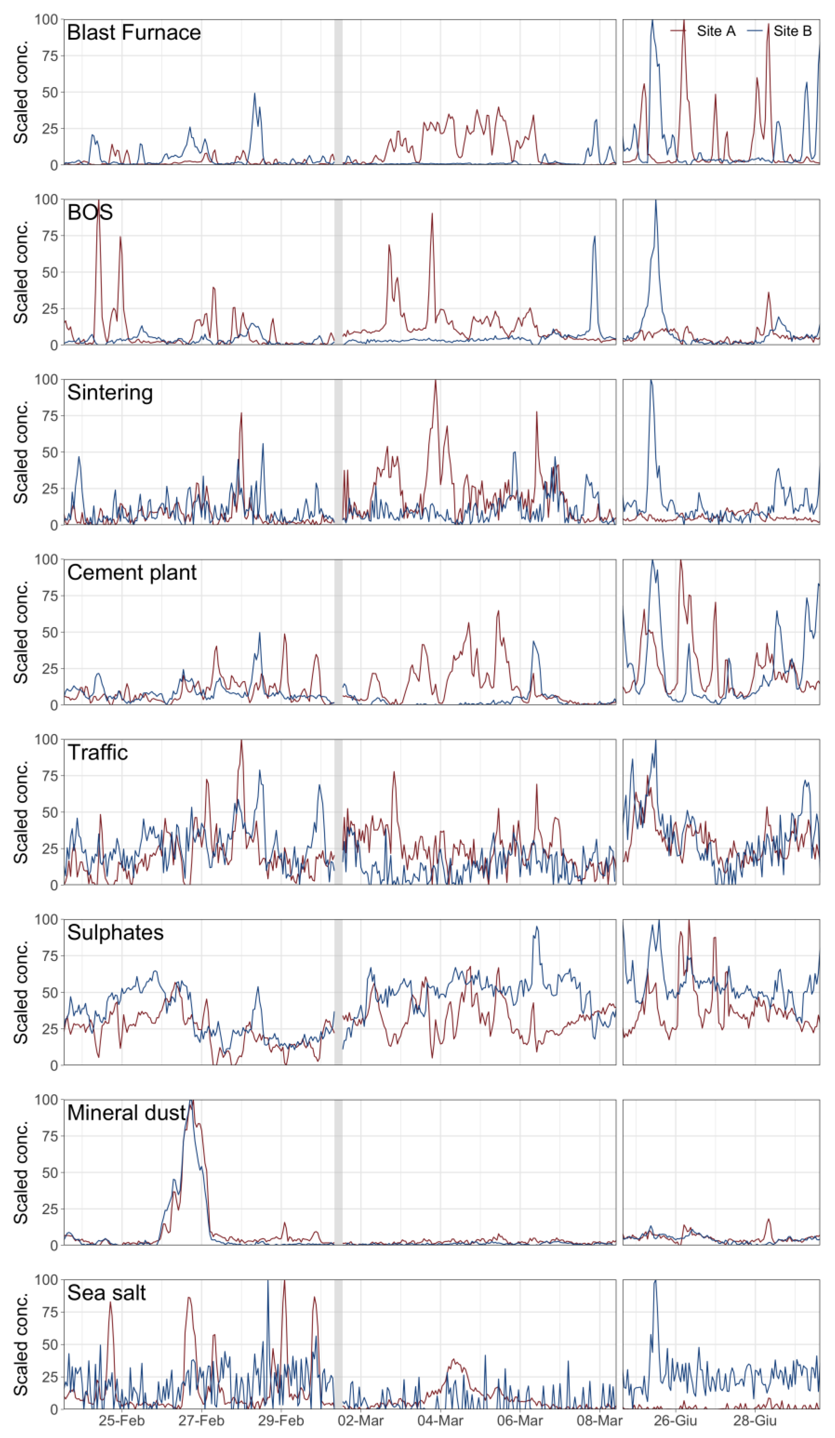
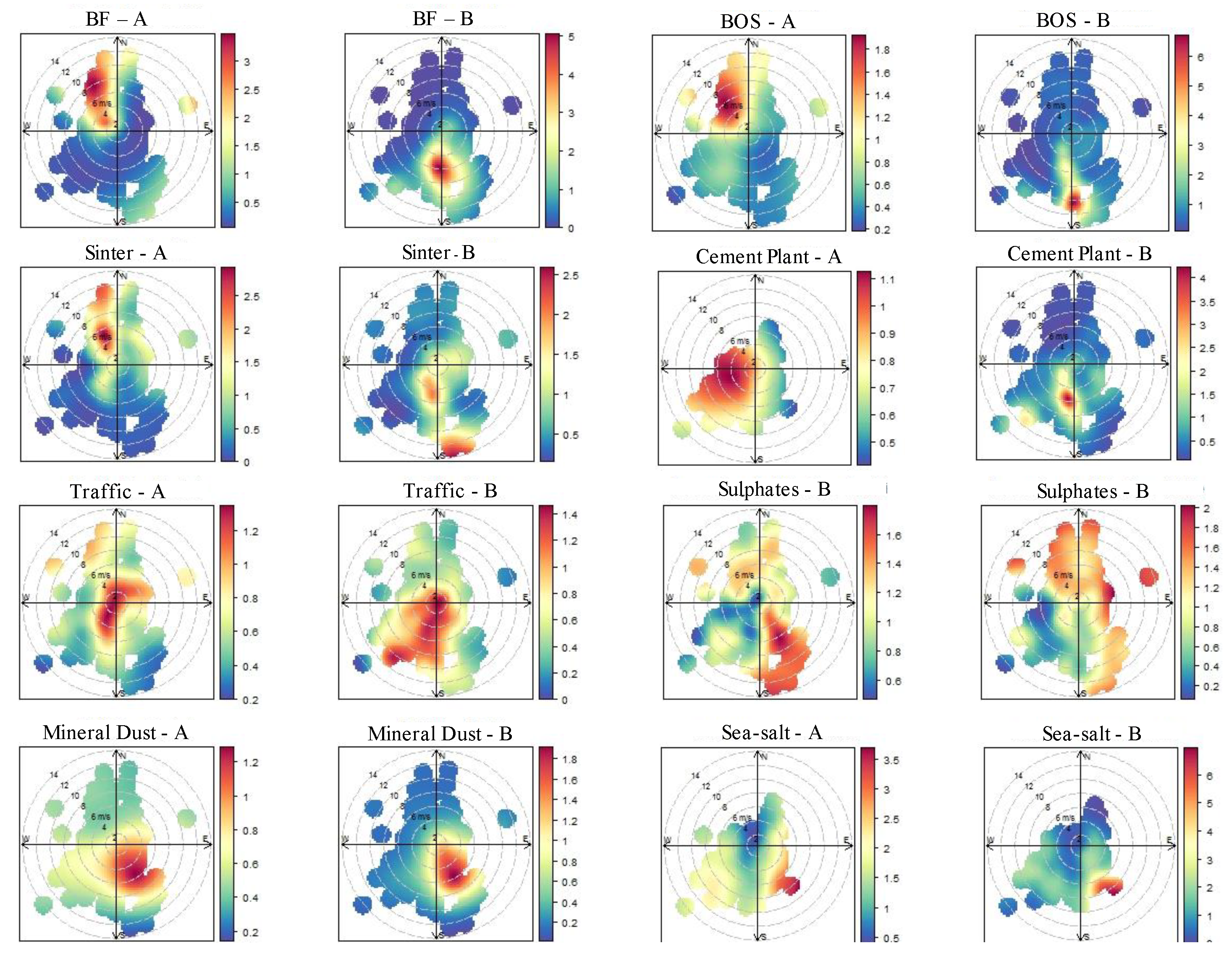
3.2. Source Apportionment

The source apportionment analysis of the PIXE data was carried out by the Positive Matrix Factorization (PMF) EPA5 software package. Since the measurements of the PM mass in the samples are not available, only relative temporal trends of source contributions in arbitrary units and the contribution to each measured element due to the identified sources can be obtained. The mean of the contribution of each source is normalized to one.
For the fine fraction, PMF analysis was applied to a matrix of 17 chemical species (16 for the coarse fraction) in 614 samples. According to the signal-to-noise ratio, all the variables (the elements) were selected as good, except V, Ni and Sr in the fine fraction, and Br, Sr and Pb in the coarse one, which were considered as weak variables.
The solution with 8 sources and 6 sources, respectively, in the fine and in the coarse fraction, and FPEAK = 0 were the most reasonable (with Q/Qexpected 1.2 and 1.3 in the fine and in the coarse fraction, respectively). The scaled residuals were normally distributed and between ±3 for all the species. A very good correlation (r2 in the range 0.87–0.99) between measured and modelled elemental concentrations was found and elements were reconstructed within 20% (i.e., modelled to measured concentration ratio in the range of 0.82–1) in both fractions, except for the weak variables (but the peaks in the concentrations of those elements were well reconstructed). Since no direct information on the mass of streaker samples is available, it is not possible to obtain an absolute source apportionment with a calculation of the errors of the obtained contributions through the Bootstrap (BS) or Displacement (DSP) methods; however, BS and DSP are useful to test the stability of the identified sources. The solutions are stable as the largest observed drops of Q during DISP are low (−0.004 and −0.07 for the fine and the coarse fraction, respectively) and no swaps were observed among the factors neither in the DSP nor in the BS analysis.
Finally, 8 and 6 factors were selected for the fine and coarse fraction respectively, because with one factor less, there is a clear mixture of two different sources, with at least one element not well reconstructed (e.g., in the coarse fraction with only 5 factors, one is a mixture of aged sea-salt and traffic and Cu shows a bad correlation, r2 = 0.37, between measured and modelled elemental concentrations and a slope equal to 0.32). With one more factor, the new one is a mixture of many elements with no physical meaning, with swaps in the BS analysis and elements different from 0 in the DSP matrix in the third and fourth rows.
Average source contributions to elemental concentrations, in ng/m3 (left axis, blue columns) and in percentage of measured elemental concentrations (right axis, red points) are reported in Figure 6 (fine fraction) and Figure 7 (coarse fraction). Actually, the source profiles reported in these figures are not true absolute profiles, as we did not normalize to the total aerosol mass. They are elemental source apportionments (in ng/m3 and %).
In Figure 8, the temporal patterns of the identified factors in the fine fraction are represented in arbitrary units for both sites. The homologous sources show a similar trend in the coarse fraction. The polar plots are presented in Figure 9 for a better identification of the different emission sources. They are produced correlating the PMF results of the streaker hourly data together with the wind data (speed and direction). The distance from the center in the graphs is proportional to the wind speed, the angle represents the wind direction and the color of each sector represents the source strength averaged over all the hours in which the wind has blown in that direction with that speed [16,17].
The factors identified in the fine fraction were: blast furnace (BF), basic oxygen system (BOS), sintering, cement plant, traffic, sulphates, mineral dust and sea salt. The factors identified in the coarse fraction were: BF, cement plant, traffic, mineral dust, fresh sea-salt, aged sea-salt. BOS, Sintering and Sulphates factors were found only in the fine fraction, whilst the sea-salt factor splits into two contributions (fresh and aged) in the coarse one. The assignment of the factor profiles detected by PMF to physical sources was done according to the considerations reported hereinafter.
Factor 1 is labeled as blast furnace (BF) due to the high percentage of Fe and Mn in this factor and the dominance of iron concentration in the chemical profile [18,19,20,21,22,23,24] as a result of furnace tapping and slag quenching operations. S is removed in the pig iron by making use of Mn and lime (hence the possible origin of some Ca in the profile). The same source was found both in the fine and in the coarse fraction. It is worth noting that the impact of the BF source is characterized by sharp peaks occurring at different times at the two locations (Figure 8), as it could be expected due to the location of the industrial area with respect to the sampling sites. The temporal behavior observed highlights the usefulness for high-resolution techniques when studying such a kind of emissions.
The polar plots are consistent with the BF location with respect to the measuring sites (southerly sector from the site B and northwesterly sector from site A) and show a narrow directional sector, pointing at the existence of pollution plumes from this plant.
Factor 2 is associated with the basic oxygen steelmaking, BOS (from steelmaking, charging, blowing and tapping) due to the presence of Zn as the marker element (more than 60% of Zn is due to this factor). Indeed, the use of galvanized scrap in the BOS has been reported to increase Zn concentrations in the steelworks processing section [5,18,20,25]. The polar plots (Figure 9) again are consistent with the BOS location with respect to the measuring sites and show a narrower directional sector. This source is present only in the fine fraction (note that Zn is mainly in the fine fraction, see Figure 2).
The profile of factor 3 is characterized by the presence of Fe, K and Pb (75% of Pb is explained by this factor). The association of these elements with emissions by the stack of the sinter plant has already been emphasized by several authors in the literature [18,19,25,26,27,28]. This factor is present only in the fine fraction. The polar plots (Figure 9) are consistent with the sinter plant location with respect to the measuring sites.
Factor 4 is characterized in both fractions by Ca and S and it is likely to include contributions from a cement kiln [29,30] located on the westerly sector with respect to sampling site A (see Figure 9) and in the southerly sector with respect to sampling site B. The source polar plots (Figure 9) confirm this association. Also, a contribution from urban soil dust (due, for example, to other anthropogenic activities such as construction, demolition works and releases from buildings and other surfaces through weathering and other erosive processes or earth-moving operations) can be present. Scarce precipitation limits the cleansing of paved surfaces and, as a result, re-suspension is favored.
The high percentage of Cu due to factor 5 together with the contribution of S and soil-related elements suggest a possible association with traffic emissions [4,31,32,33]. Likely, these are mainly non-exhaust emissions due to both heavy-duty traffic in the steelworks area, and traffic on major and minor roads. Cu, Fe, Mn and Zn are normally associated with vehicle wear particles [34], tire, engine and brake wear particles [4], while Al, Si, Ca, Ti and Fe can be associated to dust re-suspension by traffic [35]. The time pattern of this source is not as regular as in other urban areas since there is a strong contribution of heavy-duty vehicles from the industrial areas during the whole day. The source polar plots show both a local contribution and one coming from the nearby highway, the harbor and the industrial area.
The chemical profile of the sixth factor (present only in the fine fraction) was mainly defined by Sulphur, which derives from SO2 oxidation in gas to particle conversion processes. Stationary continuous coke-making emissions and blast furnace can be related to the high S concentrations (e.g., References [28,36,37]), which are rich in SO2 [20]. The SO2 emissions can favor the formation of sulphate aerosol and consequently, its accumulation on metals emitted by different iron- and steel-making processes. In addition to sources located in the steelworks area, source polar plots suggest that this factor is also expected to be associated with long-distance transport or a regional background contribution of sulphates, mainly in the form of ammonium sulphate, and to shipping and power plant emissions as contributing sources due to the high loadings of Ni and V, established tracers for oil combustion and coal combustion [29,34].
Factor 7 represents the crustal contribution, given that it is defined by typical soil elements, such as Al, Si, Ca, K, Ti Fe, Mn and Sr [31,38,39,40]. Enrichment factors with respect to Al calculated for this source following the Mason approach [41] are all close to 1 for all the crustal elements. The stronger contribution is around 26 February, on both sites. As already shown in Section 3.1, this peak is due to a Saharan dust intrusion as confirmed by the HYSPLIT Model calculations, which show that air masses are coming from Sahara and arrive from the SE, and by the source polar plots. Intermittent fugitive emissions from steelworks related with the unloading, stocking and wind entrainment of raw materials could also contribute to this factor, but there is not a clear steelworks contribution to this factor looking at the source polar plots (Figure 9).
Last factor is labelled as sea-salt aerosol, according to the high percentage of Na and Cl, which are typical markers for sea salt ([42] and the references therein). As expected, the marine factor (Figure 9) is strongly associated with south-westerly/south-easterly winds and its impact can be seen at both sites. In the coarse fraction (where this factor is more relevant, as deduced by the distribution of the concentrations of Na and Cl in the fine and coarse fraction, see Figure 2), this factor is split into two factors, the freshly emitted “sea-salt” and the “aged sea-salt”. Actually, in the fine fraction, the Mg/Na and the S/Na ratios are close to the typical ones of bulk seawater (Mg/Na = 0.12, S/Na = 0.07, [43]). The Cl depletion is 72% and 96% respectively, in the fine fraction and in the coarse aged one. Therefore, the sea-salt factor in the fine fraction can also be defined as an aged sea-salt. The Cl depletion is due to a well-known chemical reaction between gaseous species and sea-salts, where the Cl depletion is balanced by an enrichment of nitrates and sulfates. Two reactions that might be responsible for the Cl disappearance are:
HNO3 + NaCl ⇒ NaNO3 + HCl,
H2SO4 + 2NaCl ⇒ Na2SO4 + 2HCl
In both cases, particles rich in Na are obtained as a result. The obtained “aged sea-salt” profile evidenced some trace metals contribution such as S, Fe, Cu, K, Ni and V, which confirm an anthropogenic contribution.
As shown in Figure 10, elements were found to be well distributed among the sources. The sea-salt sources contributed in most of Na and Cl in both fractions and majorly in Mg, S and Br in the coarse one, the mineral dust source for Al, Si and Ti, the cement plant in Ca, the BF in Fe and Mn, the traffic in Cu and, only for the fine fraction, the sulphate in S, K, V and Ni, BOS in Zn and Sintering in Pb. Therefore, industrial activities influence most of the trace metals.

4. Conclusions

The emissions from integrated steel-making facilities are complex. The proximity of the main steelworks processes makes it difficult to distinguish individual processes. Identification is further complicated both by the influence of other external anthropogenic activities and by the simultaneous presence of continuous and discontinuous processes over time. Because of the non-continuous nature of many steelmaking processes, daily filter sampling does not have sufficient time resolution to capture short-lived events arising from specific emissions.
The hourly data collected at the two sites in Taranto area allowed us to observe in detail the different emissions from the integrated steel-making facility and was proven to be indispensable in resolving contributions from different steelworks units, a discrimination that the daily data would not have been able to detect due to the short time characterizing these emissions. The location of the sampling sites, in opposite position with respect to the industrial site, allowed us to follow the impact of the industrial plume as a function of wind direction. Moreover, the hourly resolution demonstrated high metal concentrations lasting a few hours, which may lead to an exposure problem in this area. The presence of other anthropogenic and natural sources was also identified. The receptor model analysis has allowed the identification of 8 factors for the fine fraction and 6 factors for the coarse one. The source polar plots were able to identify the directional locations of different sources identified by PMF. The source profiles obtained in our work can be useful as a reference for future source apportionment studies in similar areas.
Contributions not identified by the use of the hourly data alone (e.g., secondary nitrates) are due to the lack of suitable markers. It is thus desirable to combine hourly resolution data on different chemical components (e.g., elements, ions, carbonaceous components and, possibly, the aerosol mass) and chemical profiles for daily data to obtain a complete characterization of the aerosol sources and an absolute source apportionment.

Author Contributions

Conceptualization, F.L. and S.N.; Formal Analysis, F.L. and S.N.; Investigation, F.L., S.N.; Methodology, M.C., C.C.; Measurements: F.L., S.N. and M.C.; Data Curation, F.G. and G.C.; Writing—Original Draft Preparation, F.L.; Writing—Review and Editing, F.L., S.N., F.G., C.C., M.C. and. G.C.; Visualization, F.G.; Supervision, F.L.; Project Administration, F.L.; Funding Acquisition, F.L. All authors have read and agreed to the published version of the manuscript.

Funding

This research was funded by the Italian Health Ministry and ISPESL.

Acknowledgments

We are deeply indebted to Patrizia Di Filippo and Claudio Gariazzo (ISPESL) for their kind collaboration.

Conflicts of Interest

The authors declare no conflict of interest.

References

  1. Seshadri, S. (Ed.) Treatise on Process Metallurgy, Volume 3: Industrial Processes, 1st ed.; Elsevier: Amsterdam, The Netherlands, 2013. [Google Scholar]
  2. ILVA. Available online: https://en.wikipedia.org/wiki/Ilva(company) (accessed on 15 April 2020).
  3. Italy Chronicles. Available online: http://italychronicles.com/italy-killer-steelworks/#sthash.ON9o8c28.dpuf (accessed on 9 March 2020).
  4. Pant, P.; Harrison, R.M. Estimation of the contribution of road traffic emissions to particulate matter concentrations from field measurements: A review. Atmos. Environ. 2013, 77, 78–97. [Google Scholar] [CrossRef]
  5. Sylvestre, A.; Mizzi, A.; Mathiot, S.; Masson, F.; Jaffrezo, J.L.; Dron, J.; Mesbah, B.; Wortham, H.; Marchand, N. Comprehensive chemical characterization of industrial PM2.5 from steel industry activities. Atmos. Environ. 2013, 152, 180–190. [Google Scholar] [CrossRef]
  6. PIXE International Corporation. Available online: https://www.bloomberg.com/profile/company/0143609D:US (accessed on 20 April 2020).
  7. Chiari, M.; Del Carmine, P.; Garcia Orellana, I.; Lucarelli, F.; Nava, S.; Paperetti, L.R. Hourly elemental composition and source identification of fine and coarse PM10 in an Italian urban area stressed by many industrial activities. Nucl. Instrum. Methods Phys. Res. Sect. B Beam Interact. Mater. Atoms. 2006. [Google Scholar] [CrossRef] [Green Version]
  8. Calzolai, G.; Chiari, M.; García Orellana, I.; Lucarelli, F.; Migliori, A.; Nava, S.; Taccetti, F. The new external beam facility for environmental studies at the Tandetron accelerator of LABEC. Nucl. Instrum. Meth. B 2006, 249, 928–931. [Google Scholar] [CrossRef]
  9. Maxwell, J.A.; Teesdale, W.J.; Campbell, J.L. The Guelph PIXE software package II. Nucl. Instrum. Meth. B 1995, 95, 407–421. [Google Scholar] [CrossRef]
  10. Paatero, P.; Tapper, U. Positive matrix factorization: A non-Negative factor model with optimal utilization of error estimates of data values. Environmetrics 1994, 5, 111–126. [Google Scholar] [CrossRef]
  11. D’Alessandro, A.; Lucarelli, F.; Mandò, P.A.; Marcazzan, G.; Nava, S.; Prati, P.; Valli, G.; Vecchi, R.; Zucchiatti, A. Hourly elemental composition and source identification of fine and coarse PM10 particulate matter in four Italian towns. J. Aerosol Sci. 2003, 34, 243–259. [Google Scholar] [CrossRef]
  12. Polissar, A.V.; Hopke, P.K.; Paatero, P.; Malm, W.C.; Sisler, J.F. Atmospheric aerosol over Alaska 2. Elemental composition and sources. J. Geophys. Res. 1998, 103, 19045–19057. [Google Scholar] [CrossRef]
  13. Kfoury1, A.; Ledoux1, F.; Roche, C.; Delmaire, G.; Roussel, G.; Courcot, D. PM2.5 source apportionment in a French urban coastal site, under steelworks emission influences using constrained non-negative matrix factorization receptor model. Int. J. Environ. Sci. 2016, 40, 114–128. [Google Scholar] [CrossRef]
  14. Mazzei, F.; D’Alessandro, A.; Lucarelli, F.; Marenco, F.; Nava, S.; Prati, P.; Valli, G.; Vecchi, R. Elemental composition and source apportionment of particulate matter near a steel plant in Genoa (Italy). Nucl. Instrum. Meth. B 2006, 249, 548–551. [Google Scholar] [CrossRef]
  15. Draxler, R.R.; Rolph, G.D. HYSPLIT Model, NOAA ARL READY. 2003. Available online: http://www.arl.noaa.gov/ready/hysplit4.html (accessed on 19 April 2020).
  16. Carslaw, D.C. The Openair manual-Open-Source tools for analysing air pollution data. In Manual for Version 0.8-0; King’s College: London, UK, 2013. [Google Scholar]
  17. Carslaw, D.C.; Ropkins, K. Openair-An R package for air quality data analysis. Environ. Model Softw. 2012, 27–28, 52–61. [Google Scholar] [CrossRef]
  18. Hleis, D.; Fernandez-Olmo, I.; Ledoux, F.; Kfoury, K.; Courcot, L.; Desmonts, T.; Courcot, D. Chemical profile identification of fugitive and confined particle emissions from an integrated iron and steelmaking plant. J. Hazard. Mater. 2013, 250–251, 246–255. [Google Scholar] [CrossRef] [PubMed]
  19. Tsai, J.H.; Lin, K.H.; Chen, C.Y.; Ding, J.Y.; Choa, C.G.; Chiang, H.L. Chemical constituents in particulate emissions from integrated iron and steel facility. J. Hazard. Mater. 2007, 147, 111–119. [Google Scholar] [CrossRef]
  20. Dall’Osto, M.; Booth, M.J.; Smith, W.; Fisher, R.; Harrison, R.M. Study of the size distributions and the chemical characterization of airborne particles in the vicinity of a large integrated steelworks. Aerosol. Sci. Tech. 2008, 42, 981–991. [Google Scholar] [CrossRef] [Green Version]
  21. Mazzei, F.; D’Alessandro, A.; Lucarelli, F.; Nava, S.; Prati, P.; Valli, G.; Vecchi, R. Characterization of particulate matter sources in an urban environment. Sci. Total Environ. 2008, 401, 81–89. [Google Scholar] [CrossRef] [PubMed]
  22. Moreno, T.; Jones, T.P.; Richards, R.J. Characterisation of aerosol particulate matter from urban and industrial environments: Examples from Cardiff and Port Talbot, South Wales, UK. Sci. Total Environ. 2004, 334–335, 337–346. [Google Scholar] [CrossRef]
  23. Connell, D.P.; Winter, S.E.; Conrad, V.B.; Kim, M.; Crist, K.C. The Steubenville Comprehensive Air Monitoring Program (SCAMP): Concentrations and solubilities of PM2.5 trace elements and their implications for source apportionment and health research. J. Air Waste Manag. 2006, 56, 1750–1766. [Google Scholar] [CrossRef] [Green Version]
  24. Taiwo, A.M.; Beddows, D.C.S.; Calzolai, G.; Harrison, R.M.; Lucarelli, F.; Nava, S.; Shi, Z.; Valli, G.; Vecchi, R. Receptor modelling of airborne particulate matter in the vicinity of a major steelworks site. Sci. Total Environ. 2014, 490, 488–500. [Google Scholar] [CrossRef] [Green Version]
  25. Oravisjarvi, K.; Timonen, K.L.; Wiikinkoski, T.; Ruuskanen, A.R.; Heinanen, K.; Ruuskanene, J. Source contributions to PM2.5 particles in the urban air of a town situated close to a steel works. Atmos. Environ. 2003, 37, 1013–1022. [Google Scholar] [CrossRef]
  26. Yang, H.H.; Lee, K.T.; Hsieh, Y.S.; Luo, S.W.; Huang, R.J. Emission Characteristics and Chemical Compositions of both Filterable and Condensable Fine Particulate from Steel Plants. Aerosol. Air Qual. Res. 2015, 15, 1672–1680. [Google Scholar] [CrossRef] [Green Version]
  27. Zhan, G.; Guo, Z. Basic properties of sintering dust from iron and steel plant and potassium recovery. J. Environ. Sci. 2013, 25, 1226–1234. [Google Scholar] [CrossRef]
  28. Almeida, S.M.; Lage, J.; Fernández, B.; Garcia, S.; Reis, M.A.; Chaves, P.C. Chemical characterization of atmospheric particles and source apportionment in the vicinity of a steelmaking industry. Sci. Total Environ. 2015, 521–522, 411–420. [Google Scholar] [CrossRef] [PubMed]
  29. Kim, E.; Hopke, P.K.; Edgerton, E.S. Source Identification of Atlanta Aerosol by Positive Matrix Factorization. J. Air Waste Manag. 2003, 53, 731–739. [Google Scholar] [CrossRef] [PubMed] [Green Version]
  30. Yubero, E.; Carratalá, A.; Crespo, J.; Nicolás, J.; Santacatalina, M.; Nava, S.; Lucarelli, F.; Chiari, M. PM10 source apportionment in the surroundings of the San Vicente del Raspeig cement plant complex in southeastern Spain. Environ. Sci. Pollut. Res. 2011, 18, 64–74. [Google Scholar] [CrossRef]
  31. Dall’Osto, M.; Querol, X.; Amato, F.; Karanasiou, A.; Lucarelli, F.; Nava, S.; Calzolai, G.; Chiari, M. Hourly elemental concentrations in PM2.5 aerosols sampled simultaneously at urban background and road site. Atmos. Chem. Phys. 2013, 13, 4375–4392. [Google Scholar]
  32. Moreno, T.; Karanasiou, A.; Amato, F.; Lucarelli, F.; Nava, S.; Calzolai, G.; Chiari, M.; Coz, E.; Artiano, B.; Lumbreras, J.; et al. Daily and hourly sourcing of metallic and mineral dust in urban air contaminated by traffic and coal-burning emissions. Atmos. Environ. 2013, 68, 33–44. [Google Scholar] [CrossRef]
  33. Lucarelli, F.; Chiari, M.; Calzolai, G.; Giannoni, M.; Nava, S.; Udisti, R.; Severi, M.; Querol, X.; Amato, F.; Alves, C.; et al. The role of PIXE in the AIRUSE project “testing and development of air quality mitigation measures in Southern Europe. Nucl. Instrum. Methods Phys. Res. B 2015, 363, 92–99. [Google Scholar] [CrossRef]
  34. Thorpe, A.; Harrison, R.M. Sources and properties of non-Exhaust particulate matter from road traffic: A review. Sci. Total Environ. 2008, 400, 270–282. [Google Scholar] [CrossRef]
  35. Amato, F.; Alastuey, A.; Karanasiou, A.; Lucarelli, F.; Nava, S.; Calzolai, G.; Severi, M.; Becagli, S.; Gianelle, V.; Colombi, C.; et al. AIRUSE-LIFE: A harmonized PM speciation and source apportionment in five southern European cities. Atmos. Chem. Phys. 2016, 16, 3289–3309. [Google Scholar] [CrossRef] [Green Version]
  36. Pacyna, J.M. Atmospheric emissions of arsenic, cadmium, lead and mercury from high temperature processes in power generation and industry. In Lead, Mercury, Cadmium and Arsenic in the Environment; Hutchinson, T.C., Meema, K.M., Eds.; John Wiley and Sons Ltd.: Hoboken, NJ, USA, 1987. [Google Scholar]
  37. Pancras, J.P.; Landis, M.S.; Norris, G.A.; Vedantham, R.; Dvonch, J.T. Source apportionment of ambient fine particulate matter in Dearborn, Michigan, using hourly resolved PM chemical composition data. Sci. Total Environ. 2013, 448, 2–13. [Google Scholar] [CrossRef]
  38. Almeida-Silva, M.; Almeida, S.M.; Freitas, M.C.; Pio, C.A.; Nunes, T.; Cardoso, J. Impact of Sahara dust transport on Cape Verde atmospheric element particles. J. Toxicol. Environ. Health Part A 2013, 76, 240–251. [Google Scholar] [CrossRef] [Green Version]
  39. Nava, S.; Becagli, S.; Calzolai, G.; Chiari, M.; Lucarelli, F.; Prati, P.; Traversi, R.; Udisti, R.; Valli, G.; Vecchi, R. Saharan dust impact in central Italy: An overview on three years elemental data records. Atmos. Environ. 2012, 60, 444–452. [Google Scholar] [CrossRef]
  40. Rodríguez, S.; Calzolai, G.; Chiari, M.; Nava, S.; García, M.I.; Lopez-Solano, J.; Marrero, C.; Lopez-Darias, J.; Cuevas, E.; Alonso-Perez, S.; et al. Rapid changes of dust geochemistry in the Saharan Air Layer linked to sources and meteorology. Atmos. Environ. 2020, 223, 117186. [Google Scholar]
  41. Mason, B. Principles of Geochemistry, 3rd ed.; Wiley: New York, NY, USA, 1966. [Google Scholar]
  42. Viana, M.; Kuhlbusch, T.A.J.; Querol, X.; Alastuey, A.; Harrison, R.M.; Hopke, P.K. Source apportionment of PM in Europe: A review of methods and results. J. Aerosol. Sci. 2008, 39, 827–849. [Google Scholar] [CrossRef]
  43. Seinfeld, J.H.; Pandis, S.N. Atmospheric Chemistry and Physics—From Air Pollution to Climate Change; Hoboken, N.J., Ed.; John Wiley: Hoboken, NJ, USA, 1998. [Google Scholar]
Figure 1. Location of the industrial area and of the sampling sites on the Taranto area map.
Atmosphere 11 00419 g001
Figure 2. Box and whisker plot of the elemental concentrations in two sampling sites for the fine (upper) and the coarse (lower) fractions. Boxes indicate the inter-quartile range, black horizontal lines are average values and the ends of the whiskers represent the 10th and 90th percentiles.
Atmosphere 11 00419 g002
Figure 3. Temporal trends (in ng m−3) of Fe measured simultaneously at the two sites in the fine fraction.
Atmosphere 11 00419 g003
Figure 4. HYSPLIT backward trajectories ending at Taranto at 12 UTC on 26 February at 500, 1500 and 2500 m a.s.l., corresponding to the peak in the soil-related elements (see text for the details).
Atmosphere 11 00419 g004
Figure 5. Temporal trends (in ng m−3) of Sulphur (S) measured simultaneously at the two sites in the fine fraction.
Atmosphere 11 00419 g005
Figure 6. Source profiles obtained by positive matrix factorization (PMF) analysis of the fine fraction dataset: contribution of each species to the chemical profile composition of each source (ng/m3, blue bars) and average percentage contribution of each source to the concentration of each element (%, red diamonds).
Atmosphere 11 00419 g006
Figure 7. Source profiles obtained by PMF analysis of the coarse fraction dataset: contribution of each species to the chemical profile composition of each source (ng/m3, blue bars) and average percentage contribution of each source to the concentration of each element (%, red diamonds).
Atmosphere 11 00419 g007
Figure 8. The temporal patterns of the identified factors in the fine fraction (in arbitrary units) in both the sampling sites.
Atmosphere 11 00419 g008
Figure 9. Source polar plots as a function of wind direction and speed in site A and site B for the 8 sources identified in the fine fraction.
Atmosphere 11 00419 g009
Figure 10. Distribution of the chemical species between the sources identified by PMF in the fine fraction (above) and in the coarse one (below).
Atmosphere 11 00419 g010

