Article

Pillars of Solution for the Problem of Winter PM2.5 Variability in Fresno—Effects of Local Meteorology and Emissions

by
Thishan Dharshana Karandana Gamalathge
1,*,
Mark C. Green
1 and
William R. Stockwell
1,2
1
Division of Atmospheric Sciences, Desert Research Institute, Reno, NV 89512, USA
2
Department of Physics, The University of Texas at El Paso, El Paso, TX 79968, USA
*
Author to whom correspondence should be addressed.
Atmosphere 2020, 11(3), 312; https://doi.org/10.3390/atmos11030312
Submission received: 24 February 2020 / Revised: 16 March 2020 / Accepted: 20 March 2020 / Published: 23 March 2020
(This article belongs to the Special Issue Atmospheric Aerosols in North America)

Abstract

:
The mass composition of Particulate Matter (PM) with an aerodynamic diameter of 2.5 microns (PM2.5) in San Joaquin Valley (SJV) is dominated by ammonium nitrate (NH4NO3), a secondary pollutant. The goal of this research was the investigation of the relationship between emissions, meteorology and PM2.5 concentrations in Fresno for the winter season. It was found that location of sites near emission sources such as freeways compared with residential sites strongly affected measured PM2.5 concentrations. It was found that although long-term trends showed declines in both emissions and PM2.5 concentrations, there was substantial variability between the years in the PM2.5–emissions relationship. Much of the yearly variation in the relationship between emissions and PM2.5 concentrations can be attributed to yearly variations in weather, such as atmospheric stability, precipitation frequency and average wind speed. There are moderate correlations between PM2.5 concentrations and temperature differences between nearby surface stations at varying elevations which explains some of the daily and seasonal variation in PM2.5. Occurrence of precipitation was related to low PM 2.5, although the higher wind speeds and lower atmospheric stability associated with precipitation likely explain some of the low PM2.5 as well as washout of PM.

1. Introduction

Particulate Matter (PM) is a major contributor to poor air quality in the San Joaquin Valley (SJV; [1,2]). The SJV covers the lower portion of central California, extending downward from Sacramento through Fresno until it ends in the Tehachapi Mountains north of Los Angeles (Figure 1). Valleys limit pollutant dispersion and dilution and therefore the topography of the SJV is a factor that contributes to the high PM concentrations, especially during winter [3]. Van Donkelaar et al. [4] found high PM2.5 (PM with an aerodynamic diameter of <2.5 microns) concentrations across the SJV and the Los Angeles metropolitan area. High spatial contrast in PM2.5 is expected due to diverse land cover/use and terrain features and the land–sea interface. California showed a more pronounced PM2.5 spatial variation than the eastern U.S. [4,5]. Fresno, a major city in the SJV, has high PM2.5 concentrations. Schauer and Cass [6] analyzed source contributions of PM2.5 in Fresno and found 43% of the observed PM2.5 was due to direct emissions (primary in origin). Much of the mass composition of the PM in the SJV is ammonium nitrate (NH4NO3; [7,8,9]). Pun and Seigneur [10] showed that during the wintertime, NH4NO3 constitutes 30% of urban PM2.5 and 60% of rural PM2.5 in SJV.
Meteorology has a strong effect on the chemistry of NH4NO3 formation. To form NH4NO3 particles, oxides of nitrogen (NOX) must be converted to nitric acid (HNO3) through photochemical processes and through nighttime gas-phase and heterogeneous chemistry. Photochemical reactions during the day produce the hydroxyl radical (HO), and the reaction of NO2 with HO is the most important source of HNO3 formation during the daytime [11]. Gaseous ammonia (NH3) and gaseous HNO3 react to form ambient particulate NH4NO3.
NH3(g) + HNO3(g) ⇔ NH4NO3(g)
NH4NO3(g) ⇔ NH4NO3(s)
This equilibrium depends on temperature and relative humidity (RH; [12]). Increasing temperature leads to an increasing rate of dissociation of NH4NO3(s) and remains constant for a given temperature below deliquescence RH [13]. Above the deliquescence RH, increasing RH leads to rapid decreases in dissociation.
Transport and mixing of emissions affect NH4NO3 formation times and these depend on windspeed, terrain, synoptic conditions and other factors. Smith and Lehrman [14] showed that surface transport distances are insufficient to mix NH3 emissions with NOx emissions to form secondary NH4NO3 in SJV, and so wind speed has a minor effect on PM2.5 formation. Precipitation may also have a strong effect on PM concentrations [15]. Mixing height of the atmospheric boundary layer is expected to be important because of its effects on the concentrations of gas-phase chemical species and PM [16].
Chow and Watson [7] developed a conceptual model for winter PM2.5 episodes in the SJV that includes widespread transport of HNO3 above the planetary boundary layer at nighttime that reacts with NH3 emissions from agricultural areas to form NH4NO3 which is then mixed to the surface after radiative heating causes turbulent mixing in late morning. Using data from 38 sites in the SJV, Chow et al. [17] calculated “zones of representation” for PM2.5, elemental carbon (EC) and NH4NO3 within which the given pollutant varied by ±20%. For Fresno, the zone of representation was 10 km for PM2.5, 18 km for NH4O3 and <1 km for EC. This suggests that the nitrate is due to regional sources and the EC due to local sources.
Green et al. [18] found moderate correlations (r2 = 0.4−0.6) between heat deficit (a vertical stability quantifier) and PM2.5 at several cities in the western United States. However, the heat deficit method cannot be determined for Fresno because there are no radiosonde or other long-term measurements of vertical temperature structure. In Reno, Nevada, daily variation in winter daily average PM2.5 was moderately correlated to daily average temperature difference between a site on the valley floor and a slope-side site a few hundred meters above the valley floor (r2 = 0.42 for winter 2008–2009 to r2 = 0.785 for winter 2009–2010) [19].
The purpose of this current work was to examine the relationship between emissions, atmospheric stability, precipitation and PM2.5 in Fresno. For an example, PM2.5 concentrations could be estimated if there was a high correlation between PM2.5 concentrations and the surface temperature difference between nearby sites at varying elevations.

2. Methods

2.1. Characteristics of Selected Sites and Databases

Fresno County was chosen for our analysis because it has a large population of 989,255 that is exposed to poor air quality [20]. Therefore, in this study, we focused on how meteorological variables and emissions affect ambient PM2.5 concentrations at sites in Fresno County, California. Table 1 shows the sites we used to obtain PM2.5 data while Table 2 shows the obtain we used to get meteorological data. No new monitoring was conducted for this study—existing air quality and meteorological databases were used. Locations of all sites are shown in Figure 2. Garland is located in the middle of a large residential area. Fresno-Garland is an active super site, with an extensive amount of data, including chemically speciated data since 2004. Clovis is close to a freeway and approximately 14 km north of Garland. Fancher Creek is approximately 14 km north of Clovis, and Trimmer is approximately 15 km north of Fancher Creek. The analysis of data extending between the years 2000 to 2016 was made separately for each of these four sites. We accounted for the background of each separately, which makes the findings site specific. Although a more extensive analysis was made for Fresno-Garland due to the greater amount of available data, it should not be assumed to be representative of all the four sites because each site has different topographic features. Another factor that complicates our multiyear analysis of PM2.5 concentrations is due to the fact that there have been many emissions reduction programs implemented in California over the last two decades. However, these programs allow some evaluation of the impact of the emission reductions on PM2.5 concentrations.
The winter season was defined from November of the shown year to February of the next year.

2.2. Analyses

Atmospheric stability is a meteorological factor that we expect to be correlated with PM2.5 concentrations in the SJV. There are several methods/techniques to provide atmospheric stability information—radiosondes, rawinsondes, Radio Acoustic Sounding System (RASS), the difference between air and soil temperature, and the difference in temperature between the site of interest and nearby meteorological sites at different elevations. Among all, the most common method to obtain upper air observations is radiosondes, but a radiosonde site does not exist in SJV. So based on data availability, we converted temperature to potential temperature and used the potential temperature difference between sites to determine the atmospheric stability.
Three different types of plots of hourly average PM2.5 values were plotted for the Fresno-Garland and Clovis-Villa sites to analyze the PM2.5 variability patterns. The plots were:
  • Hour of the day of each month in each winter (2015–2017) averaged together,
  • Hour of the day of same months in different winters averaged together (Note: Black color curves in Figure 3, Figure 4 and Figure 5), and
  • Hour of the day of all months in all winters averaged together.
We examined how topographical, meteorological, and emission conditions affected PM2.5 concentrations in the SJV. We looked at how the level of PM2.5 varies with surface temperature difference, wind speed, precipitation, and emissions. Since radiosonde data or other vertical temperature data was not available for Fresno, we examined using temperature differences between sites at different elevations as a stability measure.
Emission data for Fresno was obtained from the California Air Resources Board (CARB; [27]). CARB defines the base year of 2012, which means the 2012 inventory year was based on actual/real inventory data and is the anchoring year for hind-casting and forecasting inventory years using growth and controlled factors [28]. In this work, we considered emissions of reactive organic gases (ROGs), ammonia (NH3), oxides of nitrogen (NOx), sulfur oxides (SOx), carbon monoxide (CO), and PM. The inventory contains data for different source types—stationary, areawide, mobile, and natural. Data was downloaded for Fresno County for each winter season from 2000 to 2016. The CARB emissions data used was for winter months, determined by CARB as from November to April.
Temperature gradients for Clovis, Fancher Creek and Trimmer were examined, with the Fresno-Garland site used as the reference site. To better relate to atmospheric stability, we considered the difference in potential temperature between the sites. A potential temperature difference that is positive between a higher altitude site and a lower altitude site corresponds to stable atmospheric conditions, while negative potential temperature difference represents an unstable atmosphere. The relationships between the PM2.5 concentrations measured at the Garland site and potential temperature gradients for winters 2015 through 2017 were examined in detail. The 24 h average PM2.5 and 24 h average temperature values were available for the Garland site, but other sites had temperature data with much higher temporal resolution. Mostly, there were three to four readings per every hour, and this allowed computation of daily averages for the Clovis, Fancher Creek and Trimmer sites.

3. Results

For some understanding of the nature of PM2.5 in Fresno, first we consider the chemical composition of the aerosol, chemically speciated PM2.5 data that is available at Fresno since 2004. The average percent of each major component of PM2.5 is shown in Table 3:
Ammonium nitrate and organic mass (=1.4* organic carbon) dominate PM2.5 at Fresno.
Next, we present patterns of PM2.5 and their relationship to meteorology for the winters of 2015–2017. After that, we consider how winter average PM2.5 varied with emissions and meteorology over the long term (winter 2001–winter 2017).

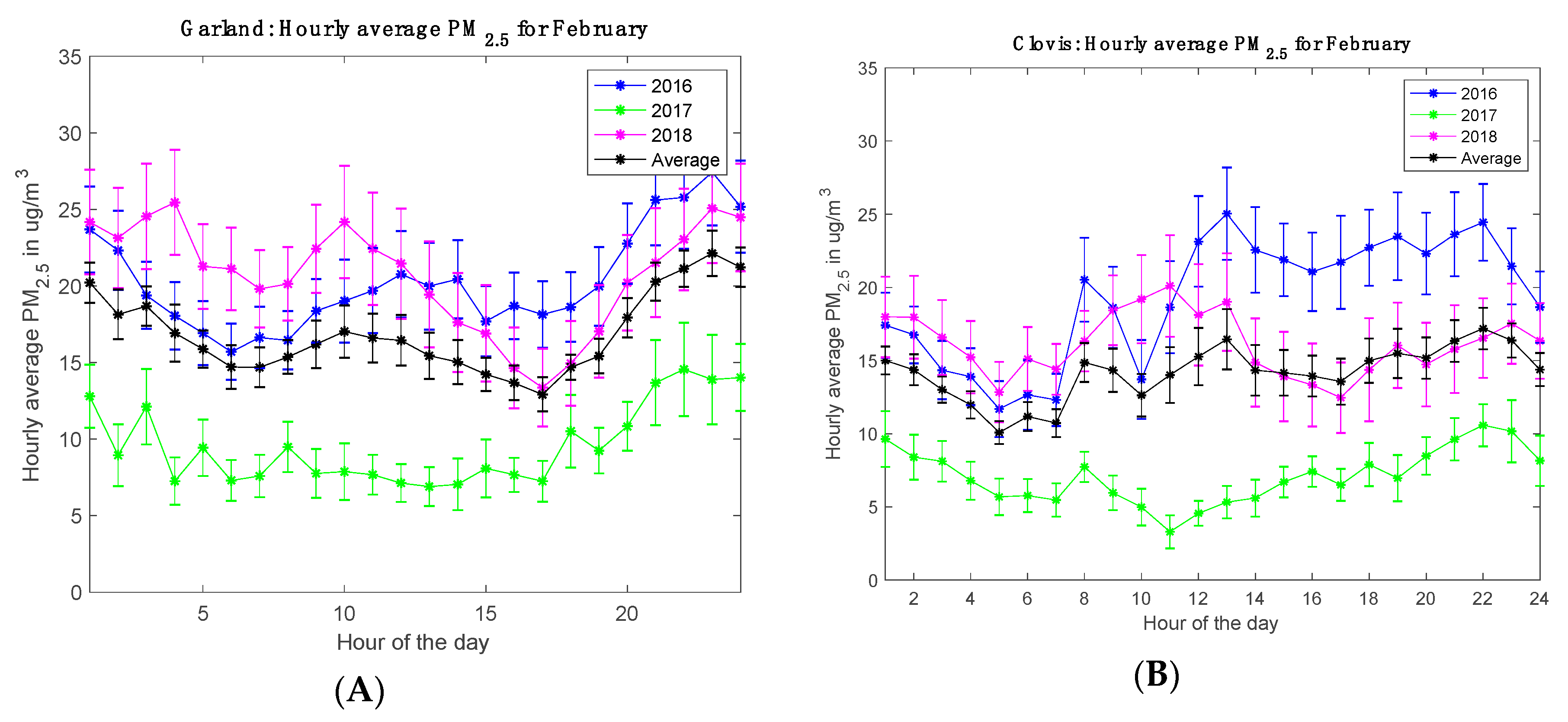
3.1. Hourly Average PM2.5 Variation for Garland and Clovis during Winter Months

Figure 3 and Figure 4 show that the Garland and Clovis sites have high PM2.5 concentration for December 2017 and January 2018. It is not clear which year had the lowest concentrations occurring simultaneously at both sites during the month of December. Except for a few hours for Garland in January 2017, the lowest concentration for both sites for both January and February (Figure 5) occurred in 2017. We do not show November here because the diurnal patterns were not clear.
With all winters averaged together, the hourly average PM2.5 variation for both sites is shown in Figure 6. The figure shows that the Garland and Clovis sites have quite similar hourly PM2.5 variation ranges. Although the Garland and Clovis sites are only approximately 4 km apart, hourly PM2.5 patterns are different. Garland has the lowest PM2.5 in the afternoon, while Clovis has the lowest in the morning. However, if we consider the scale, then the morning and afternoon lowest levels for Clovis are approximately the same.
The Figure 2 shows that the Clovis site is near the edge of a freeway, while the Garland site is in a community/residential area approximately 2 km away from the freeway. The morning increase in PM2.5 between 7 and 9 a.m. in Garland is approximately 1 µg/m3 while for Clovis, there is a sharp increase of 3 µg/m3. This is likely because Clovis receives direct contributions from morning traffic. The daily buildup in PM2.5 concentrations at Garland occurs over a time period of approximately 3 h, while at Clovis it lasts approximately 6 h. The morning rise of PM2.5 in Garland occurs between 7:00 and 10:00 a.m. while for Clovis, the increase begins at 7: 00 a.m. but it extends to approximately 1:00 p.m. The longer period at Clovis is probably due to continuing freeway traffic.
The PM2.5 concentrations at Garland decrease gradually between 10:00 a.m. and 3:00 p.m. while for Clovis, the concentrations decrease more sharply between 1:00 p.m. and 4:00 p.m. This could be due to the effect of traffic on the freeway on surface convection and turbulence.
The sharp increase in PM2.5 from 06:00 to 20:00 for Garland is most likely due to the combination of residential heating and cooking activities, while the increase from 8:00 p.m. to midnight is probably due to heating. However, for Clovis, the increase in PM2.5 from 16:00 to 22:00 is probably due to the continuation of afternoon/evening traffic. Traffic on the freeway drops significantly after 10:00 p.m. and it reflects on the Clovis site by a continuous drop of PM2.5 level. From mid-night to 7:00 a.m., the PM2.5 level further drops for both sites but the level of PM2.5 is higher for the Garland site due to residential heating. Both sites might have affected from the inversion layer to the same degree because there is only a 10 m elevation difference.

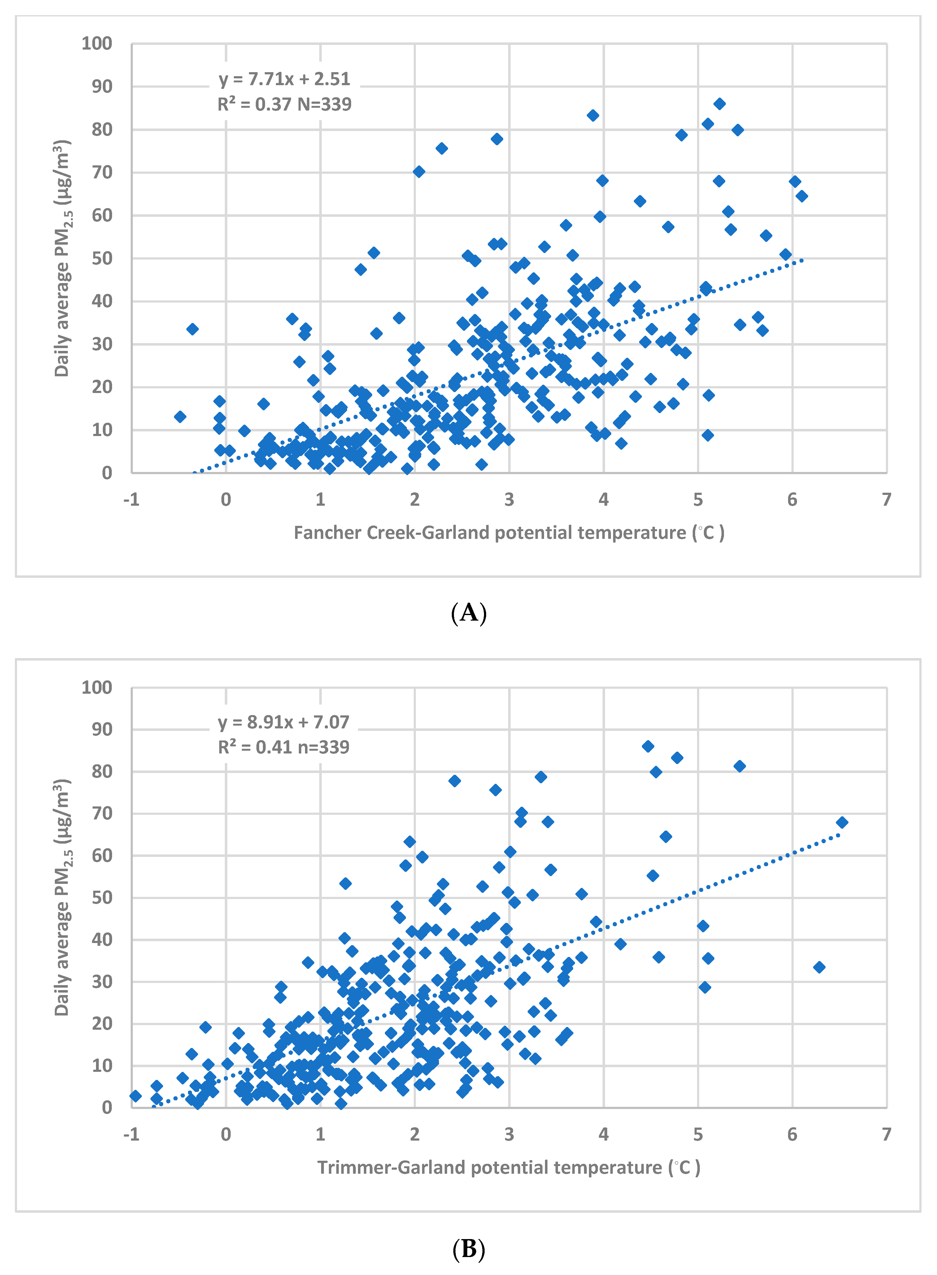
3.2. The Relationship Between PM2.5 Concentrations and Potential Temperature Gradients

As shown in Figure 7, there are moderate correlations (r2 = 0.37−0.41) between PM2.5 at Garland and potential temperature difference between Garland and elevated sites (Table 4). This suggests that PM2.5 levels are to some extent dependent upon this measure of atmospheric stability as would be expected. These squared correlations are approximately comparable to those obtained between PM2.5 and heat deficit for other locations such as Boise, Idaho (0.31−0.46), Reno, Nevada (0.53–0.59) and Salt Lake City, Utah USA (0.44–0.53) [7].

3.3. The Relationships among Wind Speed and Precipitation and PM2.5

Because potential temperature gradients showed only a moderate relationship with PM2.5, we now consider other meteorological factors and how they relate to PM2.5. Wind speed is expected to decrease PM2.5 concentrations due to along-wind dispersion. Precipitation is expected to decrease PM2.5 levels due to washout of Particulate Matter. Daily PM2.5 concentrations versus Trimmer–Garland daily average potential temperature, Garland temperature, wind speed and precipitation amount are plotted in Figure 8.
Figure 8 shows that PM2.5 is positively correlated with Trimmer–Garland potential temperature, has essentially zero correlation with Garland temperature, and is inversely correlated with wind speed and precipitation.
Average PM2.5 concentrations, average Trimmer–Garland potential temperature differences, precipitation frequency and average wind speeds are shown for each month for each year for the winters of 2015–2017 in Table 5.
December, 2017 and January, 2018 had the highest average PM2.5 concentrations of any months in the three winter periods examined, far exceeding the PM2.5 levels in the December and January of the other two years. These months also had higher potential temperature differences, lower wind speeds and lower precipitation frequencies compared to the December and January in the other two years. The winter of 2017 (November 2017–February 2018) had the highest average PM2.5, potential temperature difference, lowest frequency of precipitation and lowest wind speed of the three winters. The three Novembers had very similar average PM2.5 concentrations and relatively similar values for the other factors. February 2017 had the lowest PM2.5 of the three winters and also had the lowest potential temperature difference, greatest precipitation frequency and highest wind speed. It appears that use of potential temperature difference, precipitation frequency and wind speed together can explain why some months and years are especially high or low in PM2.5. Later, we show that potential temperature difference, precipitation frequency and wind speed are also related (precipitation days have higher winds speeds and less potential temperature differences compared to dry days).

3.4. Emission Inventory, Meteorology and PM2.5 Concentrations at the Fresno-Garland Site

Figure 9 shows how the emissions of NOx, ROGs, NH3, PM2.5 primary emissions, SOx and total emissions related to PM2.5 concentrations over a 17 year period at the Fresno First Street and Garland sites. All these pollutants might be expected to contribute to primary or secondary PM2.5 concentrations, although formation of PM2.5 from gaseous precursors will vary greatly based on meteorological and other factors. Note that the winter season for PM2.5 measurements at Fresno is from November to February while for emission data, it is from November to April. Primary PM2.5 emissions had the highest correlation coefficient with annual average winter PM2.5 concentrations at r2 = 0.52 (r = 0.72), with other compounds having somewhat lower correlations.
Figure 9 can also be used to provide insight into the variation range of emissions (in tons/day) for different pollutants over the 17 year period; NOx (~100), ROGs (~60), PM2.5 (~15), NH3 (~5), SOx (~2). It is noticeable that the trend in the emission pattern for NH3 is different compared to other pollutants. It increases until 2011 and suddenly drops and continues at a lower level thereafter. That is because the SJV APCD Rule 4570 was applied for various farming operation categories such as dairy cattle and feedlot cattle beginning with the calendar year 2012 [29].
Apart from that, it is clear that the PM2.5 variation pattern is not smooth over the years. Gorin et al. [30] emphasized that frequent precipitation events that occurred during winter 2003 were the reason for uncommonly low PM2.5 concentrations in 2003. On the other hand, California experienced its worst drought in over a century between 2011 and 2015. The 2013–2014 winter was by far the driest winter during that time period. During drought conditions, there is less washout of PM2.5 than during more typical precipitation conditions, leading to higher PM2.5 concentrations. Air pollution generated from wildfires was enormous and resulted in periods of excessively high PM2.5 concentrations [31].
Figure 9F shows how daily average PM2.5 vary with total emissions of the pollutants together over the years. There is a clear downward trend in total emissions per year, but this is not well correlated with yearly average winter PM2.5. Thus, we next look at meteorological conditions each year to better explain the year-to-year variability in the PM2.5–emissions relationship.

3.5. Year-to-Year Variability in PM2.5 and Average Yearly Meteorological Variables

Here, we consider how meteorological variables are related to year-to-year variation in average PM2.5. As shown in Figure 9, PM2.5 emissions and PM2.5 decline over the years. The correlation coefficient (r2) between PM2.5 and PM2.5 emissions was 0.72. The correlation coefficient (r) between PM2.5 and year was −0.69 which indicates a reduction in pollution levels over the years although the shared variance (r2) was only 0.48. The r2 between PM2.5 emissions and year was 0.94, a high value indicating that year is a good proxy for PM2.5 emissions in Fresno. PM2.5 emissions decreased an average of 5.5% per year from 2000 to 2016, indicating steady progress in emission control.
First consider how meteorological variables are related to PM2.5 and each other. Previously, it was shown that for the winters of 2015 and 2016, potential temperature differences (∆θ) between the Fresno Garland site and the Trimmer site were moderately correlated to PM2.5 concentrations on a daily basis and monthly average ∆θ, wind speed and precipitation frequency helped explain year-to-year variability in monthly average PM2.5 for 2015–2017.
Values in Table 6 show that on a daily basis, PM2.5 and ∆θ are moderately correlated (r2 = 0.19). When accounting for the change in PM2.5 emissions over time, the relationship between PM2.5 and ∆θ strengthens slightly (r2 = 0.26). Ammonium nitrate and NOX emissions-weighted ammonium nitrate are also moderately correlated ∆θ (r2 = 0.27 and r2 = 0.30, respectively). PM2.5 and ammonium nitrate are highly correlated with r2 = 0.83.
Wind speed is slightly more correlated to PM2.5 than ∆θ with r2 = 0.30 (r = −0.55) for PM2.5 and r2 = 0.32 (r = −0.57) for emissions-weighted PM2.5.
Average PM2.5, ∆θ and wind speed stratified by precipitation category are shown in Table 7. Average PM2.5 decreases as precipitation increases. With increased precipitation, wind speeds also increase and ∆θ decreases. Because increased precipitation is linked to decreased stability and increased wind speed, it is difficult to determine how much of the decrease in PM2.5 is due to washout of particles versus greater vertical and along-wind dispersion implied by the ∆θ and wind speed changes.
Because gas phase and particulate ammonium nitrate equilibrium is affected by temperature, we look at the relationship between temperature and particulate ammonium nitrate. It would be expected that with higher temperatures, there would be a shift toward lower particulate nitrate.
As noted earlier, organic mass is the second most abundant component of PM2.5 in Fresno, following ammonium nitrate. Burning of wood for home heating suggests a possible link between organic aerosol and temperature. Here, we briefly consider relationships between temperature and ammonium nitrate and organic mass.
As expected, temperature was inversely related to organic mass in winter in Fresno, especially regarding daily minimum temperatures. For the winter period of 2004–2018, organic mass negatively correlated with daily minimum temperature at the Fresno airport (Figure 10) with a correlation of −0.56 (r2 = 0.31, n = 470). This seems logical as when temperatures are colder, more residential wood burning would be expected.
Somewhat unexpectedly, temperatures had a weak relationship to ammonium nitrate, with a correlation coefficient between daily average temperature and ammonium nitrate of 0.01. Ammonium nitrate had a weak positive correlation with daily maximum temperature (r = 0.14, r2 =0.02, n = 470) and weak negative correlation with daily minimum temperature (r = −0.16, r2 = 0.03, n = 470) (Figures not shown). While higher ammonium nitrate with lower minimum temperatures is consistent with expectations, higher ammonium nitrate with higher maximum temperatures is not as we would expect due to increased volatilization at higher temperatures. Factors other than temperature must have significant influence on ammonium nitrate concentrations.
Overall, there is a weak negative correlation between minimum temperature and PM2.5 (r = −0.32, r2 = 0.10), which is likely mainly due to the moderate negative correlation between organic mass and minimum temperature.
Next, we examine the relationship of PM2.5 concentrations with PM2.5 emissions and meteorological variables by year (2001–2016) for the years with all needed variables available, as shown in Table 8 and Figure 11. The z-score is the yearly number of standard deviations from the mean of each variable averaged over all years. Four of the sixteen years had a normalized PM2.5 concentration greater than 1 standard deviation from the mean (z-score >1 or <−1). The three years with normalized PM2.5 z-score > 1 (2011, 2013, 2014) all had increased stability (∆θ), lower precipitation frequency and lower wind speed than average. The one year (2003) with normalized PM2.5 z-score < −1 had decreased stability (∆θ), higher precipitation frequency and higher wind speed than average. Years with PM2.5 concentrations that significantly depart from the long-term trend can be explained by the variations in these meteorological parameters.
Yearly average emissions-normalized winter PM2.5 correlated best with precipitation frequency (r = −0.84, r2 = 0.71), followed by ∆θ (r = 0.79, r2 = 0.62) and wind speed (r = −0.67, r2 = 0.45). Multiple linear regression was performed with annual winter average PM2.5 concentrations as the dependent variable and winter average PM2.5 emissions, ∆θ, precipitation frequency and wind speed as the independent variables. The initial regression with all variables showed a shared variance (r2) of 0.884 between predicted and measured PM2.5. However, the regression coefficients were statistically significant only for PM2.5 emissions and precipitation frequency, probably due to the moderately high correlations (multicollinearity) among the meteorological variables. The regression was then performed using only PM2.5 emissions and precipitation frequency for the independent variables. The P values were less than 10−5 for each variable. The shared variance was 0.871 between predicted and observed PM2.5. The comparison of predicted and measured PM2.5 by year is shown in Figure 12. Because PM2.5 emissions and year are highly correlated (r = −0.97, r2 = 0.94), prediction of PM2.5 using only year and precipitation frequency in the regression gave similar results as using PM2.5 emissions and precipitation frequency (r2 = 0.852).

4. Conclusions

A key goal of this research was to investigate the relationship between emissions, meteorology and PM2.5 concentrations in Fresno for the winter season. The Garland and Clovis sites have quite similar hourly PM2.5 concentration variation ranges. For the winters of 2015–2017, the highest PM2.5 concentrations occurred during December 2017 and January 2018. These months also had high atmospheric stability, light winds and little precipitation. The PM2.5 concentration and its diurnal variation at the Clovis site were strongly affected by the site’s location near a freeway compared with the Garland site. There are moderate correlations (r2 = 0.37−0.41) between PM2.5 at Garland and potential temperature difference between Garland and elevated sites, and thus stability as represented by potential temperature difference is a partial explanation for PM2.5 levels. There was strong variation in the monthly PM2.5 between the three years which could be explained by year-to-year variations in monthly precipitation frequency, atmospheric stability and wind speed. Precipitation and wind speed, in addition to potential temperature difference, can also help explain PM2.5 levels. Because these parameters are correlated with each other, it is not possible to determine the relative importance of each factor in affecting PM2.5 levels. Year-to-year monthly PM2.5 levels and annual variations in PM2.5 levels can be largely explained by considering emissions levels, atmospheric stability (∆θ), precipitation frequency and wind speed.

Author Contributions

This paper was written by T.D.K.G., with a significant contribution by M.C.G. and W.R.S. All authors have read and agree to the published version of the manuscript.

Funding

This research received no external funding.

Acknowledgments

William R. Stockwell thanks the U.S. Department of Commerce, National Oceanic and Atmospheric Administration, and Educational Partnership Program under Agreement No. NA16SEC4810006 for supporting his contributions to this research project.

Conflicts of Interest

The authors declare no conflicts of interest.

References

  1. Cisneros, R.; Brown, P.; Cameron, L.; Gaab, E.; Gonzalez, M.; Ramondt, S.; Veloz, D.; Song, A.; Schweizer, D. Understanding Public Views about Air Quality and Air Pollution Sources in the San Joaquin Valley, California. J. Environ. Public Health 2017. [Google Scholar] [CrossRef] [PubMed] [Green Version]
  2. Ferreria, S.R.; Shipp, E.M. Historical Meteorological Analysis in Support of the 2003 San Joaquin Valley PM10 State Implementation Plan; Final Report; San Joaquin Valley Air Pollution District: Fresno, CA, USA, 2005. [Google Scholar]
  3. SJVAQPCD, San Joaquin Valley Air Pollution Control District—2018 PM2.5 SIP. 2018. Available online: https://ww3.arb.ca.gov/planning/sip/sjvpm25/2018plan/photochemmodprotocol_sjvapp.pdf (accessed on 1 December 2019).
  4. Van Donkelaar, A.; Martin, R.V.; Brauer, M.; Kahn, R.; Levy, R.; Verduzco, C.; Villeneuve, P.J. Global estimates of ambient fine particulate matter concentrations from satellite-based aerosol optical depth: Development and application. Environ. Health Perspect. 2010, 118, 847–855. [Google Scholar] [CrossRef] [PubMed] [Green Version]
  5. Lee, H.J.; Coull, B.A.; Bell, M.L.; Koutrakis, P. Use of satellite-based aerosol optical depth and spatial clustering to predict ambient PM2.5 concentrations. Environ. Res. 2012, 118, 8–15. [Google Scholar] [CrossRef] [PubMed] [Green Version]
  6. Schauer, J.J.; Cass, G.R. Source Apportionment of Wintertime Gas-Phase and Particle-Phase Air Pollutants Using Organic Compounds as Tracers. Environ. Sci. Technol. 2000, 34, 1821–1832. [Google Scholar] [CrossRef] [Green Version]
  7. Watson, J.G.; Chow, J.C. A wintertime PM2.5 episode at the Fresno, CA, supersite. Atmos. Environ. 2002, 36, 465–475. [Google Scholar] [CrossRef]
  8. Neuman, J.A.; Nowak, J.B.; Brock, C.A.; Trainer, M.; Fehsenfeld, F.C.; Holloway, J.S.; Hubler, G.; Hudson, P.K.; Murphy, D.M.; Orsini, D.; et al. Variability in ammonium nitrate formation and nitric acid depletion with altitude and location over California. J. Geophys. Res. 2003, 108, 4557. [Google Scholar] [CrossRef]
  9. SJVAQPCD, San Joaquin Valley Air Pollution Control District 2012 PM2.5 Plan. 2012. Available online: http://www.valleyair.org/Air_Quality_Plans/PM25Plan2012/CompletedPlanbookmarked.pdf (accessed on 1 December 2019).
  10. Pun, B.K.; Seigneur, C. Sensitivity of particulate matter nitrate formation to precursor emissions in the California San Joaquin Valley. Environ. Sci. Technol. 2001, 35, 2979–2987. [Google Scholar] [CrossRef] [PubMed]
  11. Stockwell, W.R.; Watson, J.G.; Robinson, N.F.; Steiner, W.; Sylte, W.W. The ammonium nitrate particle equivalent of NOX emissions for winter conditions in Central California’s San Joaquin Valley. Atmos. Environ. 2000, 34, 4711–4717. [Google Scholar] [CrossRef]
  12. Stelson, A.W.; Seinfeld, J.H. Relative humidity and temperature dependence of the ammonium nitrate dissociation constant. Atmos. Environ. 1982, 16, 983–992. [Google Scholar] [CrossRef]
  13. Tang, I.N.; Munkelwitz, H.R. Composition and temperature dependence of the deliquescence properties of hygroscopic aerosols. Atmos. Environ. 1993, 27, 467–473. [Google Scholar] [CrossRef]
  14. Smith, T.B.; Lehrman, D.E. Long-Range Tracer Studies in the San Joaquin Valley. In Regional Photochemical Measurement and Modeling Studies; Ranzieri, A.J., Solomon, P.A., Eds.; A&WMA: Pittsburgh, PA, USA, 1994; pp. 151–165. [Google Scholar]
  15. Yoo, J.-M.; Lee, Y.-R.; Kim, D.; Jeong, M.-J.; Stockwell, W.R.; Kundu, P.K.; Oh, S.-M.; Shin, D.-B.; Lee, S.-J. New Indices for Wet Scavenging of Air Pollutants (O3, CO, NO2, SO2 and PM10) by Summertime Rain. Atmos. Environ. 2014, 82, 226–237. [Google Scholar] [CrossRef]
  16. Tang, G.; Zhang, J.; Zhu, X.; Song, T.; Munkel, C.; Hu, B.; Schafer, K.; Liu, Z.; Zhang, J.; Wang, L.; et al. Mixing layer height and its implications for air pollution over Beijing, China. Atmos. Chem. Phys. 2016, 16, 2459–2475. [Google Scholar] [CrossRef] [Green Version]
  17. Chow, J.C.; Chen, L.-W.A.; Watson, J.G.; Lowenthal, D.H.; Kagliano, K.A.; Turkiewicz, K.; Lehrman, D.E. PM2.5 chemical composition and spatiotemporal variability during the California regional PM10/PM2.5 air quality study (CRPAQS). J. Geophys. Res. 2006, 111, D10S04. [Google Scholar] [CrossRef]
  18. Green, M.C.; Chow, J.C.; Watson, J.G.; Dick, K.; Inouye, D. Effects of snow cover and atmospheric stability on winter PM2.5 concentrations in western U.S. valleys. J. Appl. Met. Clim. 2015, 54, 1191–1201. [Google Scholar] [CrossRef]
  19. Chen, L.-W.A.; Watson, J.G.; Chow, J.C.; Green, M.C.; Inouye, D.; Dick, K. Wintertime particulate pollution episodes in an urban valley of the Western US: A case study. Atmos. Chem. Phys. 2012, 12, 10051–10064. [Google Scholar]
  20. U.S. Census. 2017. Available online: www.census.gov (accessed on 1 July 2017).
  21. Interagency Monitoring of Protected Environments. Available online: http://vista.cira.colostate.edu/Improve/ (accessed on 15 March 2019).
  22. Interactive Map of Air Quality Monitors. Available online: https://www.epa.gov/outdoor-air-quality-data/interactive-map-air-quality-monitors (accessed on 10 January 2018).
  23. Operating Manual, Partisol®-Plus Model 2025 Sequential Air Sampler. Available online: https://www.arb.ca.gov/airwebmanual/instrument_manuals/Documents/FRM_Manual.pdf (accessed on 16 August 2019).
  24. MesoWest. Available online: https://mesowest.utah.edu (accessed on 5 December 2016).
  25. Jacques, A.; (MESOWEST, Department of Atmospheric Sciences, University of Utah, Salt Lake City, UT, USA). Personal communication, 2020.
  26. Interagency Wildland Fire Weather Station Standards & Guidelines. Available online: https://raws.nifc.gov/sites/default/files/inline-files/pms426-3.pdf (accessed on 20 October 2019).
  27. CARB. 2018. Available online: https://www.arb.ca.gov/ei/ei.htm (accessed on 11 November 2018).
  28. Klassen, J.; (SJV Air Pollution Control District, Bakersfield, CA, USA). Personal communication, 2018.
  29. Johnson, M.; (California Air Resources Board, Sacramento, CA, USA). Personal communication, 2018.
  30. Gorin, C.A.; Collett, J.L.; Herckes, P. Wood Smoke Contribution to Winter Aerosol in Fresno, CA. JA&WMA 2006, 56, 1584–1590. [Google Scholar]
  31. PM_Plan, 2018 Plan for the 1997, 2006, and 2015 PM2.5 Standards-Appendix A. 2018. Available online: https://www.valleyair.org/pmplans/documents/2018/pm-plan adopted/A.pdf (accessed on 18 April 2019).
Figure 1. Location of San Joaquin Valley (SJV), Fresno, and a few other cities in the lower portion of central California.
Atmosphere 11 00312 g001
Figure 2. Locations of air quality and meteorology monitoring stations; Garland (USEPA), Clovis-Villa (USEPA), Clovis (CIMIS), Clovis (MESOWEST), Fancher Creek (MESOWEST), and Trimmer (MESOWEST) sites. Notes: USEPA—United States Environmental Protection Agency; CIMIS—California Irrigation Management Information System; MESOWEST—this is an archive of meteorological data across the United States.
Atmosphere 11 00312 g002
Figure 3. Hourly average PM2.5 variation for Garland (A) and Clovis (B) during December.
Atmosphere 11 00312 g003
Figure 4. Hourly average PM2.5 variation for Garland (A) and Clovis (B) during January.
Atmosphere 11 00312 g004
Figure 5. Hourly average PM2.5 variation for Garland (A) and Clovis (B) during February.
Atmosphere 11 00312 g005
Figure 6. Variation in hourly average PM2.5 when all winters are averaged together.
Atmosphere 11 00312 g006
Figure 7. The relationship between the daily average PM2.5 and the potential temperature difference between the Garland and Fancher Creek (A) and Trimmer (B) sites.
Atmosphere 11 00312 g007
Figure 8. Daily average PM2.5 at Garland versus (A) daily average Trimmer–Garland potential temperature; (B) daily average Garland temperature; (C) daily average wind speed at Fresno airport; (D) daily total precipitation at Fresno airport.
Atmosphere 11 00312 g008aAtmosphere 11 00312 g008b
Figure 9. Long-term time series of atmospheric PM2.5 level with NOx (A), ROGs (B), NH3 (C), * primary PM2.5 (D), SOx (E) emissions and total of NOx, ROGs, NH3, primary PM2.5 and SOx emissions (F). * Primary PM2.5 emissions are PM2.5 emitted directly to the atmosphere.
Atmosphere 11 00312 g009
Figure 10. Variation in organic mass with minimum temperature in Fresno.
Atmosphere 11 00312 g010
Figure 11. Z-score for winter average emissions-normalized PM2.5, Trimmer–Garland potential temperature difference, precipitation frequency and wind speed.
Atmosphere 11 00312 g011
Figure 12. Winter average measured and regression predicted PM2.5 at Fresno-Garland for the winters of 2001–2016.
Atmosphere 11 00312 g012
Table 1. Fresno area sources of Particulate Matter (PM) with an aerodynamic diameter of 2.5 microns (PM2.5) data.
StationData TypeWinter Data AvailabilityTemporal ResolutionMeasurement NotesStation Coordinates and Elevation
Site name: Fresno-GarlandAQS site ID: 06-019-0011PM2.52012
2013
2014
2015
2016
2017
Daily since 1 January 2012
Hourly since
8 January 2012
This site also has Chemical Speciation Data from the Interagency Monitoring of PROtected Visual Environments (IMPROVE) aerosol network [21]
Daily (POC = 1)—Sample collection method/instrument: * R&P Model 2025 PM2.5 sequential air sampler w/VSCC. Sample analysis method: Gravimetric
Hourly (POC = 3)—Sample collection method/instrument: Met One Beta Attenuation Monitor (BAM)-1020 mass monitor w/VSCC. Sample analysis method: Beta Attenuation.
Lat: 36.785322°
Lon: −119.774174°
Elevation: 96 m
Site name: Fresno First Street AQS site ID: 06-019-0008PM2.56 January 1999–
31 January 2012
DailyPOC = 1
For daily data prior to 2012, we used data from the First Street site, at 3425 N First St (450 m away from Garland). Sample collection method/instrument: R&P Model 2025 PM2.5 sequential air sampler w/WINS.
Sample analysis method: Gravimetric
Lat: 36.781333°
Lon: −119.773190°
Elevation: 96 m
Site name: Clovis-VillaPM2.525 November 2008–31 December 2017HourlyPOC = 3
Sample collection method/instrument: Teledyne Model 602 Beta plus w/VSCCSample analysis method: Beta Attenuation.
Lat: 36.82°
Lon: −119.72°
Elevation: 86 m
Notes: (1) POC—Parameter Occurrence Code. All PM2.5 concentration data and chemical speciation data obtained from the EPA website [22]. (2) Gravimetric analysis is a method of quantitative determination of analyte based on its mass. Beta Attenuation is a method using the amount of beta radiation absorption to determine the mass of PM in the sample. (3) VSCC—Very Sharp Cut Cyclone and WINS—Well Impactor Ninety-Six serve as particle size separation devices. * R&P—Rupprecht and Patashnick Company, Incorporated Partisol-Plus Model 2025 PM-2.5 sequential air sampler [23].
Table 2. Distance to meteorological sites from the Garland site.
Local Site Name
Fresno-Garland (USEPA)Clovis (MESOWEST)Fancher Creek (MESOWEST)Trimmer (MESOWEST)
Latitude: 36.79°
Longitude: −119.77°
Elevation: 96 m
Latitude: 36.85°
Longitude: −119.63°
Elevation: 127 m
Latitude: 36.88°
Longitude: −119.48°
Elevation: 279 m
Latitude: 36.91°
Longitude: −119.31°
Elevation: 453 m
Distance from the Garland site (kms)0142843
Notes: (1) The site labeled Clovis here is not co-located with the Clovis-Villa site listed in Table 1. (2) All these sites had temperature data with a sample resolution of 1 h, but only the Fresno-Garland site had PM2.5 data. Out of daily and hourly resolutions for PM2.5, we considered the case of a resolution of 1 h. (3) MESOWEST data was accessed through https://mesowest.utah.edu [24]. (4) Personal communication with Alexander Jacques [25] in the MESOWEST team let us know that the Clovis site is a home-type weather station owned by a private citizen, and so it does not have to adhere to any specific siting or instrumentation standards. However, the Fancher Creek and Trimmer sites are part of the US BLM (Bureau of Land Management) Remote Automatic Weather Station (RAWS) network and thus need to adhere to some set of standards given in Interagency Wildland Fire Weather Station Standards and Guidelines [26]. Based on this, temperature sensors have a range from −50 to +50 °C, with 1 °C resolution and an accuracy of +/−6 °C.
Table 3. Average percent of each major component of PM2.5, Fresno IMPROVE monitoring site in the period of 2004–2018.
NH4NO3(NH4)2SO4Organic MassECCrustalOther/Unaccounted
44.9%5.7%28.6%6.0%2.8%11.9%
Table 4. Summary of the relationship strength between PM2.5 and potential temperature gradients for different sites in Fresno.
SiteElevation (m)Distance from the Fresno-Garland Site (km)r2
PM2.5 against Potential Temperature Difference
Fresno-Garland (US EPA)96------
Fancher Cree (MESOWEST)279280.37
Trimmer (MESOWEST)453430.41
The r2 value for each site was based on data from winters in 2015 to 2017.
Table 5. PM2.5, delta θ, precipitation frequency and wind speed average by month for the winter of 2015–2017.
Month/YearPM2.5 (μg/m3)Delta θ (°C)Precipitation Frequency (%)Wind Speed
(m s−1)
November
201521.601.34183.57
201621.541.92144.02
201721.181.80134.15
December
201522.201.67274.18
201625.622.08233.94
201751.702.9532.69
January
201616.431.45524.71
201710.191.20576.42
201827.442.55174.06
February
201619.141.5073.27
20178.100.66467.21
201819.441.09124.47
Entire winter
201519.911.49253.92
201617.021.51335.28
201730.512.14113.81
Notes: (1) Precipitation frequency is the percentage of days in the month with at least 0.01 inches of precipitation recorded at the Fresno airport. Wind speed is the daily average at the Fresno airport. (2) The highest PM2.5 for each month is shown in bold. Also shown in bold for each month are the values with the most potential to contribute to high PM2.5 (e.g., highest delta θ, lowest precipitation frequency, and lowest wind speed).
Table 6. Correlation coefficients (and correlations) among PM2.5 and emissions-normalized PM2.5 and delta θ and wind speed.
ParameterDelta θ (∆θ)Wind Speed
PM2.50.19 (0.44)0.30 (−0.55)
Emissions-normalized PM2.5 *0.26 (0.51)0.32 (−0.57)
NH4NO3 **0.27 (0.52)0.22 (−0.47)
Emissions-normalized NH4NO3 ***0.30 (0.55)0.20 (−0.45)
Wind speed0.12 (−0.35)
* The emissions-normalized PM2.5 is calculated by dividing the PM2.5 concentration for each day by the yearly level of PM2.5 primary particle emissions from the CARB emissions inventory. ** NH4NO3 data is available on only one day in three, so that the days for comparing to ∆θ and wind speed are not the same days as when comparing PM2.5 to ∆θ and wind speed. *** The emissions-normalized NH4NO3 is calculated by dividing the PM2.5 concentration for each day by the yearly level of nitrogen oxide (NOX) emissions from the CARB emissions inventory.
Table 7. Average PM2.5, ∆θ and wind speed by precipitation category.
Precipitation Amount (Inches)Average PM2.5 (μg/m3)Average ∆θ (°C)Average Wind Speed (m/s)Number of Observations
<0.0132.02.23.01422
0.01–0.1018.71.45.9385
>0.1012.71.17.0230
Table 8. Yearly z-scores for emissions-normalized PM2.5, ∆θ, precipitation frequency and wind speed.
YearPM2.5/Emissions of PM2.5∆θPrecipitation FrequencyWind Speed
2001−0.53−0.30−0.150.94
2002−0.07−1.11−0.110.03
2003−1.15−0.551.280.80
2004−0.90−0.510.670.37
2005−0.20−0.09−0.600.62
2006−0.010.020.110.51
2007−0.460.090.160.04
2008−0.25−0.240.62−0.54
2009−0.29−0.730.63−0.49
2010−0.64−0.420.16−0.50
20111.140.84−1.83−1.39
20120.281.87−0.23−0.97
20132.952.59−1.84−1.37
20141.040.19−1.18−0.79
2015−0.12−0.850.510.20
2016−0.79−0.811.802.55

