1. Introduction
In contrast with the significant and steady progress in tropical cyclone (TC) track forecasts over the past few decades [
1,
2], much less improvement in TC intensity forecasts, especially in rapid intensification (RI; with an increase of maximum near-surface wind of 15 m s
−1 or a drop of minimum sea-level pressure of 42 hPa in 24 h) forecasts, has been obtained. Although the TC intensity forecast errors from several operational numerical models have been decreased to some degree [
3], there remain large uncertainties and an urgent need to identify the factors that lead to the large uncertainty of TC intensity forecasts [
4,
5,
6,
7,
8], which can guide us to further improve the forecast skill of TC intensity. An inaccurate initial profile of a TC is thought to be an important reason for the subsequent poor intensity change forecast. Both Wang [
9] and Xu and Wang [
10] pointed out that the simulated TC inner-core size is largely determined by the initial vortex size. Emanuel and Zhang [
11] indicated that the error growth during the first few days is dominated by the errors in initial vortex intensity, especially those occurring in the moisture within the inner-core [
12,
13]. Clearly, these studies emphasized the importance of the initial condition of the TC in TC intensity forecasts. It is known that the initial conditions have been significantly improved but could be further improved by using high-accuracy observations and advanced data assimilation approaches. For example, the atmospheric infrared sounder (AIRS) and its companion advanced microwave sounding unit, onboard the Aqua satellite, have provided integrated atmospheric sounding information since its launch in May 2002 [
14,
15]. Using AIRS data, the TC warm core structure can be well resolved, and a strong correlation between TC intensity and warm core strength has been identified over global ocean basins [
16]. Furthermore, the Tropical Cyclone Intensity field campaign has provided high-resolution measurements of TCs within the upper-level outflow at an altitude of nearly 18 km and the inner-core [
6,
17]. With these data, both the initial warm upper-level inner-core and the convection and latent heat release within the eyewall of Hurricane Patricia (2015) were well simulated, and the later RI forecasts were improved [
18]. All these results show that the improvement in the initial inner-core strength due to the use of high-resolution observations plays an important role in improving RI forecast skill.
Zhang et al. [
19] indicated that reducing the current-day initial-condition uncertainty by an order of magnitude can extend the deterministic forecast lead times of day-to-day weather by up to 5 days. However, TCs comprise various scales of processes, and an improvement of much less than 5 days may be obtained despite the initial uncertainty in the TC inner-core being reduced by an order of magnitude. Thus, an accurate initial condition is not enough for accurate TC intensity (and RI) forecasts. Still, advanced numerical models with fewer model errors are indispensable. Undoubtedly, the continuously increasing resolution has reduced model error to some degree and advanced numerical models. For example, the European Center for Medium-Range Weather Forecasts upgraded the horizontal resolution to ~9 km to provide the highest-resolution global operational numerical weather prediction model to date. Considering that model convergence does not occur even with grid spacing well below 1 km [
20], other approaches have also been utilized to decrease the influence of model errors on TC intensity forecasts. Specifically, the approaches of stochastically perturbed parametrized tendencies [
21], stochastic kinetic-energy backscatter scheme [
22], and analysis increments [
23] were proposed to represent model errors in operational forecast systems. These approaches have improved the accuracy and reliability of ensemble forecasts for TC intensity [
24,
25,
26].
Nevertheless, numerical models are far from perfect. Zhang and Rogers [
27] modified the vertical eddy diffusivity coefficient in the boundary layer parameterization scheme and obtained two kinds of boundary layer structures during the physics upgrades of hurricane Earl (2010). Within one structure, the simulated TC reproduced the RI as observed, while within the other structure, the simulated TC weakened briefly before resuming a slow intensification. This result stresses the importance of the boundary layer in the intensification (especially the RI) of TCs, which has also been shown in previous studies [
28,
29]. Actually, to better understand the TC structure in the boundary layer, flight observations aimed at the TC boundary layer were conducted in the South China Sea since 2009, which comprised four eyewall penetrations [
30]. To better use these observations to improve the RI forecast of a TC, some questions should be first addressed: (i) Does the uncertainty in the boundary layer influence the RI forecast uncertainty of a TC? (ii) How is the sensitivity of the RI forecast uncertainty to the errors occurring in the boundary layer? Clearly, the answers to these questions will be helpful for understanding the importance of these observations and tell us how to use these observations to improve the RI forecast skill.
In the present study, we use ensemble forecast experiments to estimate the uncertainties of the RI forecast of Typhoon Dujuan (201521) induced by the uncertainties in the boundary layer and evaluate the sensitivity of the TC intensity change to the uncertainties occurring in different areas and variables in the boundary layer. In
Section 2, the model, TC case, and experimental strategy are described in detail. Then, the sensitivity of the TC track forecast to the uncertainty is first displayed in
Section 3 to distinguish its influence on the resultant intensity change. Next, the sensitivity of the intensity change forecast is shown in
Section 4.
Section 5 demonstrates the dynamic and thermodynamic structure of the TCs in different ensemble forecast members to illustrate how the uncertainty in the boundary layer affects the RI forecast. A final summary and some discussions are presented in
Section 6.
2. Model, TC Case, and Experimental Strategy
In this study, we study Typhoon Dujuan (201521) and use the ensemble forecast experiments generated by the weather research and forecasting (WRF) model to investigate the influence of the uncertainties occurring in the boundary layer on its RI forecast. The WRF model, the TC case Dujuan (201521), and the experimental strategy are introduced below.
2.1. The WRF Model
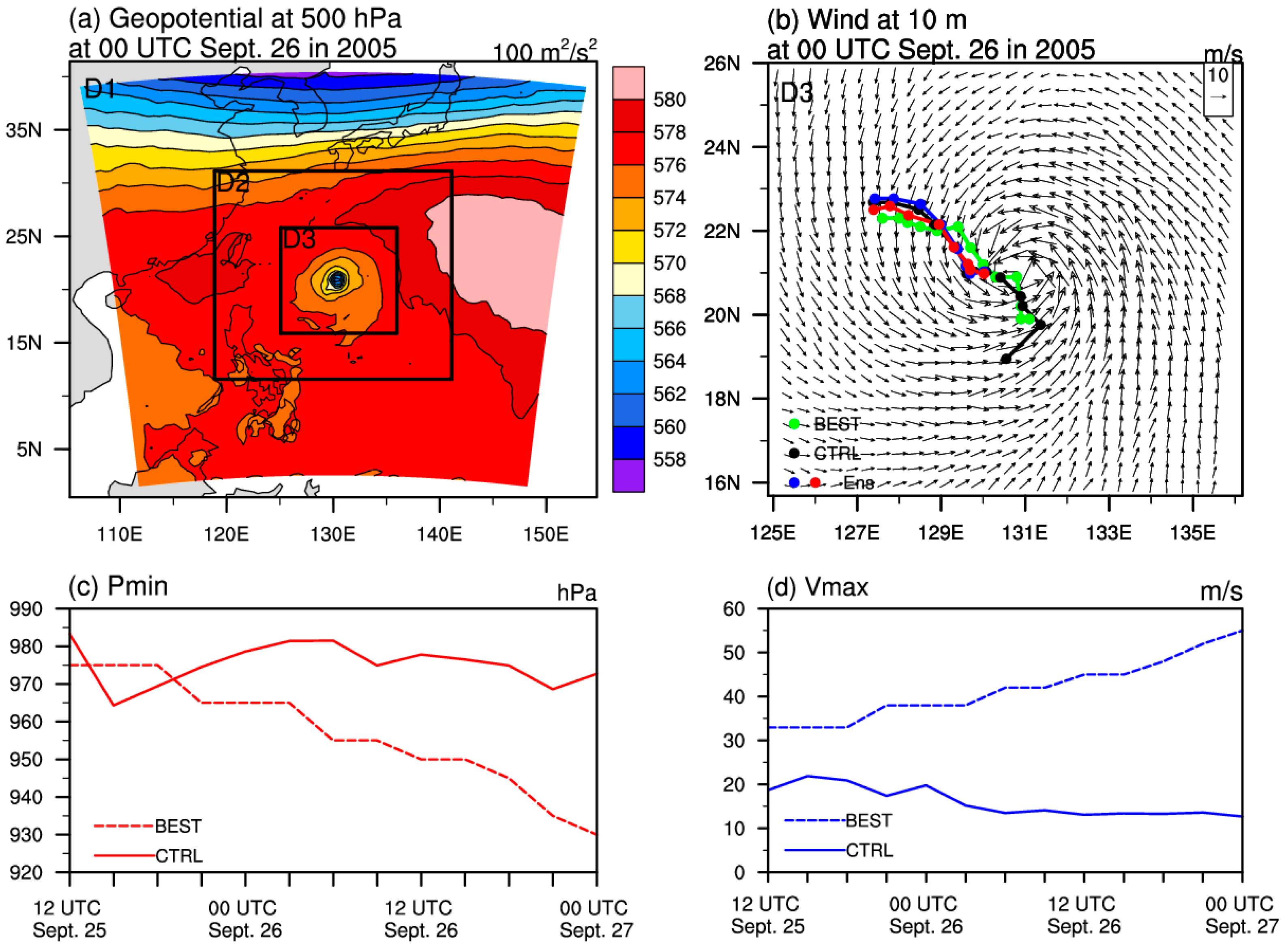
The WRF model (version 3.6) is utilized in this study, with the initial fields and boundary conditions derived from the National Centers for Environmental Prediction final reanalysis field at a resolution of 1° × 1°. The experiments are conducted in triple-nested domains, and the innermost domain is vortex following (
Figure 1a,b). The three domains, from the outermost to the innermost, have 97 × 97, 145 × 145, and 220 × 220 grid points, with grid spacings of 45, 15, and 5 km, respectively. The outermost domain (hereafter referred to as “D1”) covers a horizontal area of 4320 km × 4320 km, which is sufficient to describe mesoscale atmospheric movements. The middle domain (hereafter referred to as “D2”) covers an area of 2160 km × 2160 km, which contains the TC and parts of the synoptic systems surrounding it. The innermost domain (referred to as “D3” below), nested in D2, covers an area of 1095 km × 1095 km, which contains the structure of the TC (the eye, eyewall, gale area, etc.). The vertical grid meshes include 35 levels in the terrain-following eta coordinate from the surface to 20 hPa, with enhanced vertical resolution below a height of 1 km. All of the domains share the same parameterization schemes, which include the Kain–Frisch cumulus parameterizations except in the innermost domain [
31], Lin microphysics scheme [
32,
33], RRTMG for longwave and shortwave radiation schemes [
34], and Yonsei University (YSU) planetary boundary layer parameterization scheme [
35].
2.2. The TC Case: Typhoon Dujuan (201521)
The impact of the uncertainty occurring in the boundary layer on the TC intensity and its RI forecast is considered in the present study, which makes a TC case undergoing the RI in reality necessary. Typhoon Dujuan (201521), which originated over the western North Pacific, moved northwestward, and finally made landfall in China, is adopted here. Typhoon Dujuan (201521) was first identified as a tropical storm at 18 UTC Sept. 22 in 2015 and intensified gradually in the subsequent three days. From 03 UTC Sept. 26 to 00 UTC Sept. 27, it underwent RI with the maximum near-surface wind (Vmax) increasing from 38 m s
−1 to 55 m s
−1 and the minimum sea-level pressure (Pmin) decreasing from 965 hPa to 930 hPa. However, nearly all operational centers failed to forecast the RI process of this TC case in advance, which is also one of the reasons why Typhoon Dujuan (201521) is studied in the present study. We choose the period from 12 UTC Sept. 25 to 00 UTC Sept. 27 as the time window, of which the first 12 h correspond to spinning up, and the remaining 24 h correspond to our investigation. It should be noted that there is a position error between the simulation result (hereafter referred to as “CTRL”) and the best track data (referred to as “BEST” below) from the China Meteorological Administration (CMA) at the initial time (i.e., 12 UTC Sept. 25). The error is maintained at approximately 20–60 km during the subsequent 12 h. From 00 UTC Sept. 26 to 12 UTC Sept. 26, the simulated TC positions are located south of the BEST, with a position error of approximately 55 km. However, from 12 UTC Sept. 26 to 00 UTC Sept. 27, the simulated TC moves northwest of the BEST (
Figure 1b). With respect to intensity, the Pmin discrepancy between CTRL and BEST is approximately 10 hPa during the time period from 12 UTC Sept. 25 to 21 UTC Sept. 25, which then increases rapidly over time to a final 42 hPa at 00 UTC Sept. 27, with the CTRL being much weaker than the BEST (
Figure 1c). The 10 m maximum wind speed (Vmax) even cannot simulate the intensification from 00 UTC Sept. 26 to 00 UTC Sept. 27 (
Figure 1d). That is, the CTRL fails to reproduce the RI process.
2.3. Experimental Strategy
The ensemble forecast experiment is utilized to examine the sensitivity of the TC intensity and its RI to the uncertainty occurring in the boundary layer. First, the boundary layer with the YSU scheme is treated as one entity, and perturbations are superimposed on the outputs from the YSU scheme during the WRF model integration (i.e., the CTRL) at every grid point in the region concerned, where the outputs include horizontal wind U and V, potential temperature, and water vapor mixing ratio. As intermediate outputs from the YSU scheme, they are inputs for other parameterization schemes (i.e., cumulus scheme, microphysics scheme, etc.) and not the final diagnostic variables of WRF. Hence, these outputs from the YSU scheme indicate the variations of these variables after the work of the YSU scheme. In case there is uncertainty in the YSU scheme, the outputs will change accordingly depending on their sensitivity to the uncertainty. If the values of the outputs are denoted by “Ref”, the perturbations of these components are generated by taking the values from Ref × (1 − 50%) to Ref × (1 + 50%) at a Ref × 5% interval, which are superimposed at each integration step and finally obtain 20 ensemble forecast members. For simplification, we refer to the members generated by the perturbations that increase the YSU output as “IMs” and those made by the perturbations that decrease the YSU output as “DMs”. It should be noted that the perturbations change only the values of the outputs, rather than the signs. Specifically, taking the U-wind component as an example and supposing it is 0.5 m s−2 (variation per second in one timestep) at a given location and time, the perturbation values in the ensemble forecast members will range from 0.25 m s−2 to 0.75 m s−2 at a 0.025 m s−2 interval. That is, although a westerly wind tendency is either weakened or enhanced against CTRL in the ensemble forecast members, the wind direction remains westerly for all members. Since the perturbations are proportional to the outputs of the YSU scheme, which obeys principle physical laws and in dynamical balance, these perturbations strengthen or weaken the synoptic systems to some degree, but still in dynamic balance.
To consider the uncertainty in different areas denoted by D1, D2, and D3 (see
Section 2.1 and
Figure 1), we design four groups of ensemble forecast experiments, i.e., Exp-D1, Exp-D2, Exp-D3, and Exp-All. “Exp-D1” represents the ensemble forecast experiment that the perturbations are superimposed on the YSU scheme, but on the outermost domain D1 while no perturbations are superimposed on the other two model domains D2 and D3. “Exp-D2” and “Exp-D3” denote that the perturbations are only superimposed on the model domains D2 and D3, respectively, and “Exp-All” denotes when the perturbations are superimposed on all three model domains. For each group of experiments, there are a total of 21 ensemble forecast members: the 20 members generated by the 20 perturbations in the YSU scheme and the member corresponding to the CTRL.
3. TC Track Sensitivity
Some research [
12,
36] indicated that the forecast uncertainty of a TC track has a great influence on its intensity. After a TC makes landfall, it will often stop intensifying and even decay rapidly. Different forecast members of one TC track may lead to different landfall timings, which then cause differences in the intensity among the forecast members, especially between those which have already made landfall and those about to. In addition, it is possible that the ocean states below the TCs are different due to the fact that forecast track differences among ensemble members could cause some members to move over warm eddies and others to move over cold eddies [
37]. Hence, the response of the TC tracks in the ensemble forecast members to the perturbations to the YSU scheme should be first investigated.
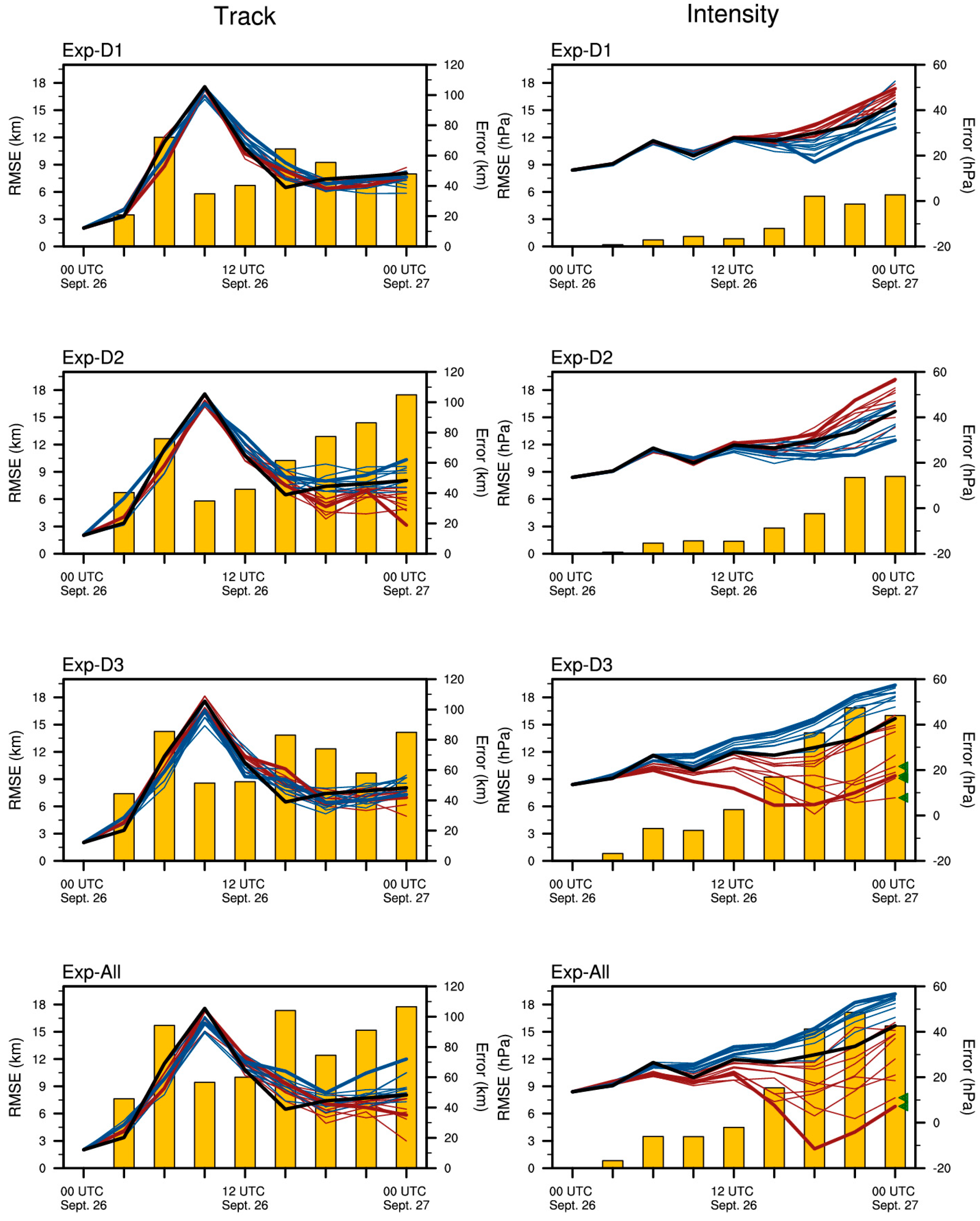
Based on the experimental strategy detailed in
Section 2, four groups of ensemble forecast experiments are conducted on Typhoon Dujuan (201521), where the perturbations to the YSU scheme are superimposed from 00 UTC Sept. 26 in 2015 and last for the subsequent 24 h. Then, the TC central positions in all the ensemble members are identified from 03 UTC Sept. 26 at a 3 h interval and the errors with respect to the best track are plotted as contours in
Figure 2. The spread (bars in
Figure 2) of TC tracks in Exp-D1, which is measured by the root mean square error (RMSE) of the 20 perturbed ensemble forecast members with respect to the CTRL, reaches a maximum of 12 km. Clearly, this spread, indicating the track difference among the ensemble forecast members, cannot be detected by the grid spacing of 45 km. However, it should be noted that the general actual track errors from the best track is about 100 km at 09 UTC Sept. 26 and decrease to 40 km at 15 UTC Sept. 26. In the steering flow area D2, both the TC and surrounding synoptic systems are better featured by the grid spacing of 15 km, then the variations of the TC with respect to the steering flow that influences TC motion are better identified among the ensemble forecast members; it is therefore that Exp-D2 exhibits a relatively large spread with the maximum of about 17 km. Further investigation is made to the tracks in two ensemble forecast members that have the most deviation (averaged over 24 h from 00 UTC Sept. 26 to 00 UTC Sept. 27) from the CTRL, with one being from the IMs and the other being from the DMs. It shows that these 24 h-averaged deviations between these two forecast tracks and that of the CTRL are less than 14 km (see
Figure 1b). That is, even for the ensemble forecast members that deviate the largest from the track in the CTRL, the absolute track difference is indeed small. This is probably because the perturbations are superimposed in the boundary layer rather than the whole troposphere. For Exp-D3, the maximum spread is up to about 13 km, in which the track differences may be a result of the impacts of small-scale processes (~5 km) on the movements of the eye areas within TC area D3. In any case, the ensemble forecast members show spreads of TC tracks less than 17 km, which is considerably smaller than the spatial scale of Typhoon Dujuan (201521) with a gale area of as large as 250 km. In addition, the statistical result from the Japan Meteorological Agency shows that the RMSE of the TC track forecasts over the western North Pacific is about 60 km for 24 h-leading time forecast, which is significantly larger than the above spread of TC tracks in ensemble forecast experiments. It is therefore that the spread of TC tracks in the above experiments are negligible, which infers that the TC tracks are less sensitive to the perturbations superimposed on the YSU scheme, regardless of the background area D1 with a grid spacing of 45 km or environmental steering flow area D2 with a grid spacing of 15 km or TC area D3 with a grid spacing of 5 km.
It should be noted that the WRF is an atmospheric model. Fixed-in-time SSTs (30 degrees) throughout the simulation period make no warm/cold-core eddy occur along the tracks. Moreover, the differences in the TC tracks among ensemble forecast members were shown to be trivial. Recalling the two situations we mentioned at the beginning of this section that the TC track influences the TC intensity, it is inferred that the variation in the intensity of Typhoon Dujuan (201521) due to the change in its track due to different ensemble forecast members is negligible.
4. TC Intensity Sensitivity
With the ensemble forecast experiments in
Section 3, the Pmin of the TC in ensemble forecast members are identified from 03 UTC Sept. 26 to 00 UTC Sept. 27 every 3 h, and their errors with respect to the BEST are shown in
Figure 2. Clearly, the spreads of TC intensity in Exp-D1 and -D2 are relatively small, and the maximum is up to about 9 hPa. According to the statistical result from the Japan Meteorological Agency [
38], the forecast error of the TC intensity is about 13 hPa for the 24 h-lead time TC forecast. That is, the spread of 9 hPa in TC intensity in the above ensemble forecast experiments is comparable to that in the operational TC intensity forecasts. For Exp-D3 and -All, the spreads become much larger with a maximum of about 17 hPa, particularly from 15 UTC Sept. 26 to 00 UTC Sept. 27. Therefore, it is reasonable to conclude that the TC intensity is generally more sensitive to the uncertainty occurring in the boundary layer represented by the YSU scheme than the TC track is. The TC intensity shows the strongest sensitivity to uncertainty occurring in the D3 region. In addition, the spread in Exp-D3 begins to increase rapidly much earlier than those in Exp-D1 and -D2, which is at 06 UTC in comparison with 15 UTC on Sept. 26 in Exp-D1 and 12 UTC in Exp-D2. It is thus inferred that the uncertainty occurring in the boundary layer associated with the TC can lead to considerable forecast uncertainty of TC intensity. In particular, there are four ensemble forecast members in Exp-D3 (see
Figure 2), but none in either Exp-D1 or Exp-D2 that successfully reproduce the RI. Furthermore, the Exp-All, considering the interaction among the uncertainties occurring in D1, D2, and D3, reproduces the RI behavior of Typhoon Dujuan (201521) in two ensemble forecast members. These comparisons show that the uncertainty occurring in the boundary layer associated with the TC area D3, rather than with the steering flow area D2 and the background environment area D1, has much greater influences on the RI forecast uncertainty for Typhoon Dujuan (201521).
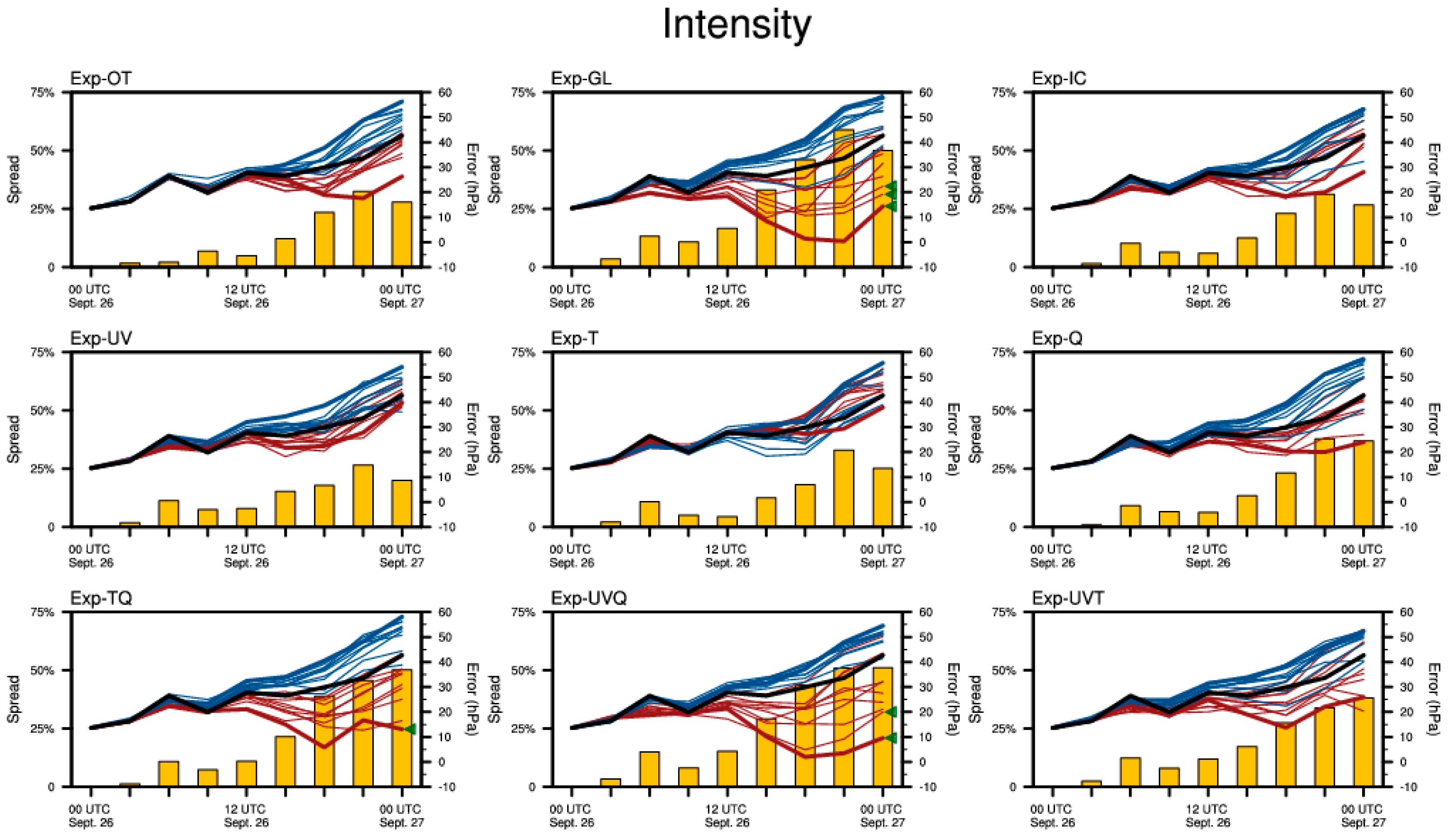
D3 covers an area of 1095 km × 1095 km and involves different parts of the TC, including the inner-core area, gale area, and outer area. Then, do the uncertainties occurring in these areas have similar influences on the TC intensity forecast? Which most strongly controls the forecast of the RI of the TC? To address these questions, another three groups of ensemble forecast experiments are constructed, which are denoted by “Exp-IC”, “Exp-GL”, and “Exp-OT”. Their only differences from the former ensemble forecast experiments are that the perturbations are superimposed in three separated areas within D3. Specifically, “Exp-IC” denotes the ensemble forecast experiments in which the perturbations in Exp-D3 are replaced by those superimposed on the YSU scheme in a circular area centered at the central position of the TC (with a radius of 55 km), which is identified according to the azimuthally averaged horizontal wind at 10 m above the surface and covers the inner-core of the TC; “Exp-GL” represents the ensemble forecast experiments in which the perturbations in Exp-D3 are replaced by those superimposed on the YSU scheme in an annular area surrounding the inner-core and with a radius between 55 km and 250 km (nearly covering the gale area), and “Exp-OT” denotes the ensemble forecast experiments in which the perturbations in Exp-D3 are replaced by those superimposed on the YSU scheme in the outer area of D3 with a distance from the center greater than 250 km (nearly covering the weak wind and buffer zones). Considering the relatively small spread of TC tracks in Exp-D3, these experiments favor evaluating the sensitivity of the TC intensity on the uncertainty occurring in different areas in D3.
The intensity forecast errors of the TC in the ensemble forecast members in Exp-OT, -GL, and -IC are shown in
Figure 3. It is shown that the ensemble forecast members in Exp-GL have distributions similar to those in Exp-D3 despite having relatively small spreads. Moreover, three members in the Exp-GL successfully reproduce the RI of the TC, but none of the Exp-OT and Exp-IC do so. Therefore, the intensity forecast uncertainty of Typhoon Dujuan (201521) shows different sensitivities to the uncertainty occurring in the boundary layer associated with different areas of the TC. The uncertainty in the boundary layer in the gale area of the TC area, compared with that in the inner-core and weak wind areas, tends to have much greater effects on the RI forecast.
The above ensemble forecast experiments are all based on the perturbations to the components of the horizontal wind, potential temperature, and water vapor mixing ratio from the outputs of the YSU scheme and do not separate the respective role of the components. The above results suggest that the perturbations superimposed in the TC area, especially in the gale area of the TC, much can easily cause large uncertainties in TC intensity. It is also the perturbations (of horizontal wind, potential temperature, and water vapor mixing ratio) superimposed in the gale area of the TC that much easily offset the uncertainty of the YSU and are helpful for improving the RI forecast skill. These results raise the following question: which component from the outputs of the YSU scheme is mainly responsible for the RI forecast? Then, another six groups of ensemble forecast experiments are conducted with perturbations superimposed on different components of the YSU scheme, but only on the gale area of the TC. These six groups of experiments are, respectively, denoted as “Exp-UV”, “Exp-T”, “Exp-Q”, “Exp-TQ”, “Exp-UVQ”, and “Exp-UVT”. Exp-UV represents the ensemble forecast experiments in which the perturbations are superimposed on the horizontal wind components (U and V) of the YSU scheme on the gale area of the TC; Exp-T and Exp-Q include the ensemble forecast experiments in which the perturbations are added to the potential temperature and water vapor mixing ratio, respectively; Exp-TQ is related to the ensemble forecast experiments in which the perturbations are added to both the potential temperature and water vapor mixing ratio; Exp-UVQ contains the ensemble forecast experiments in which the perturbations are simultaneously imposed on the horizontal wind (U and V) and water vapor mixing ratio; Exp-UVT denotes the ensemble forecast experiment in which perturbations are added to both the horizontal wind (U and V) and potential temperature.
It is shown that the perturbations superimposed on any single component of the YSU (i.e., horizontal wind (Exp-UV), potential temperature (Exp-T), and water vapor mixing ratio (Exp-Q)) cannot lead to a spread as large as that in Exp-GL (see
Figure 3). In particular, the spreads of Exp-UV and Exp-T are even smaller than those of Exp-D1, where the perturbations are superimposed on the YSU scheme in the much larger background area D1 with a grid spacing of 45 km and have been shown to be less important in causing TC intensity uncertainty. Although Exp-Q displays a relatively large spread, it is still approximately half of that of Exp-GL. Moreover, the RI is not reproduced in the ensemble forecast members in the Exp-UV, Exp-T, or Exp-Q. That is, the uncertainty associated with any single component of the outputs from the YSU scheme in the gale area is not enough to significantly disturb the TC intensity. Nevertheless, when the perturbations are simultaneously superimposed on the potential temperature and water vapor mixing ratio (i.e., Exp-TQ) or horizontal wind and water vapor mixing ratio (i.e., Exp-UVQ), the spread of the corresponding ensemble forecast members, compared with those in Exp-T and Exp-UV, increases significantly and has amplitudes similar to that of Exp-GL. More importantly, there are ensemble forecast members, specifically two in Exp-UVQ and one in Exp-TQ, that successfully reproduce the RI of the TC. In contrast, the spread of the ensemble forecast members in Exp-UVT is obviously smaller than that in Exp-UVQ and Exp-TQ. It is therefore inferred that the moisture within the gale area in the boundary layer has a very important influence on the RI of the TC, and its uncertainty, together with horizontal wind and potential temperature uncertainties, disturbs the forecast of the RI more likely.
5. Mechanism for the RI Forecast Uncertainty
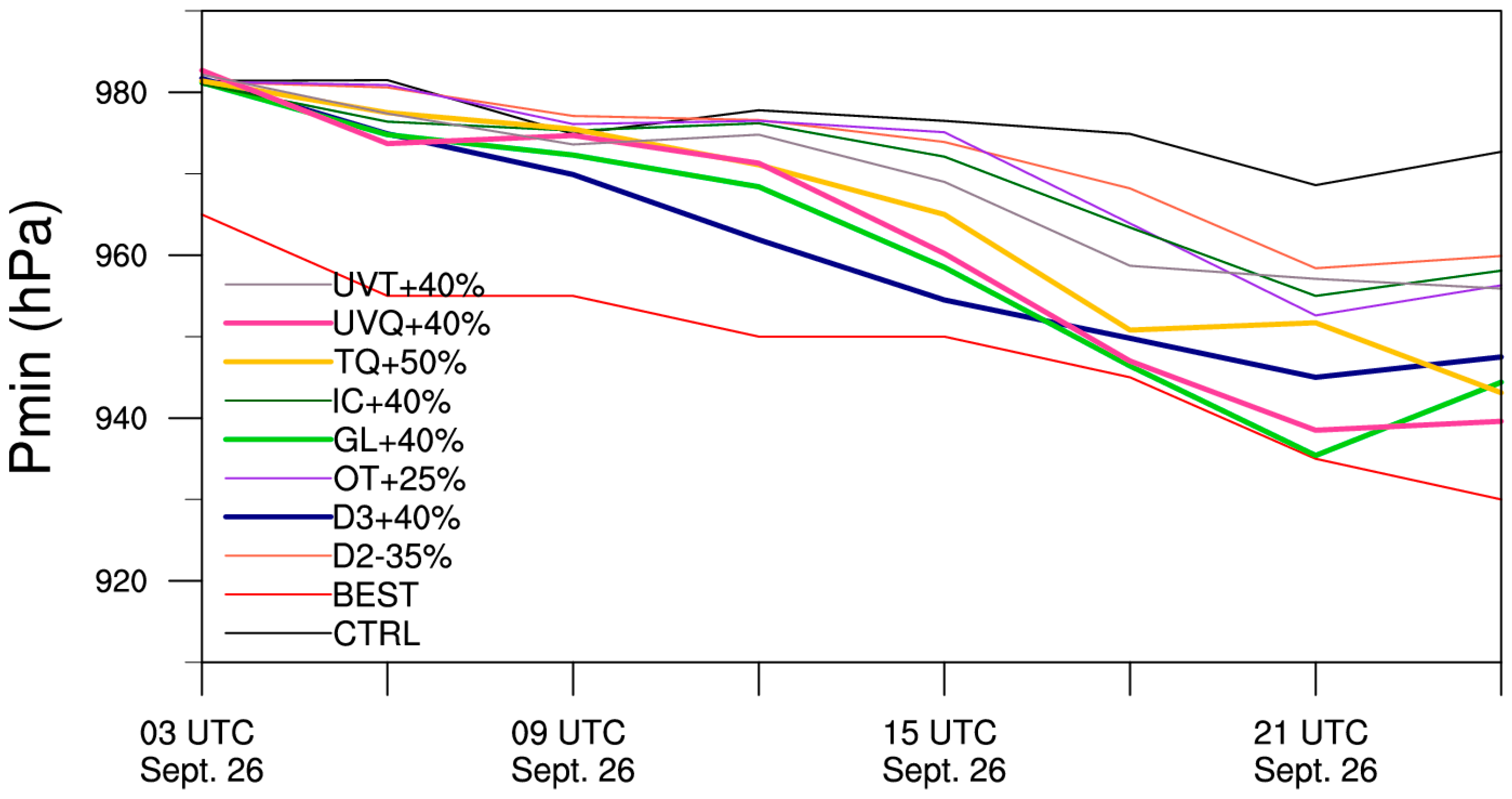
It is clear that the uncertainty occurring in the boundary layer associated with the gale area of the TC, especially with the component of the water vapor mixing ratio, contributes the most to RI forecast uncertainty of Typhoon Dujuan (201521). For this typhoon, some ensemble forecast members reproduce the RI, but others do not, which indicates that an appropriate perturbation associated with the output from the YSU scheme can offset the model errors and induce the RI as it occurs in reality. Then, how do the perturbations affect the occurrence of RI? To answer it, comparisons are made to the structures of the TCs in relevant ensemble forecast members, where the forecast TC intensities (averaged from 03 UTC Sept. 26 to 00 UTC Sept. 27) are closest to the BEST and RI occurs in some while not in others. These ensemble forecast members are referred to as “D2 − 35%”, “D3 + 40%”, “OT + 25%”, “GL + 40%”, “IC + 40%”, “TQ + 50%”, “UVQ + 40%”, and “UVT + 40%”, a total of eight members. D2 − 35% (D3 + 40%) denotes the ensemble forecast member with perturbations that proportionally decrease (increase) the outputs from the YSU scheme by 35% (40%) in the steering flow area D2 (TC area D3); IC + 40%, GL + 40%, and OT + 25% represent the ensemble forecast members with the perturbations that proportionally increase the outputs from the YSU scheme by 40%, 40%, and 25% in the inner-core, gale, and the outer portion of the TC area D3, respectively; TQ + 50% relates to the ensemble forecast member with perturbations that proportionally increase both the potential temperature and water vapor mixing ratio components of the outputs from the YSU scheme by 50% in the gale area of the TC, and similar naming schemes are used, but associate with the components of both horizontal wind and water vapor mixing ratio for UVQ + 40% and both horizontal wind and potential temperature for UVT + 40%. In particular, four members, D3 + 40%, GL + 40%, TQ+50%, and UVQ+40%, reproduce the RI process of Typhoon Dujuan (201521); while the others, i.e., D2 − 35%, OT + 25%, IC + 40%, and UVT + 40%, together with the CTRL, fail to reproduce the RI (see
Figure 4).
It is known that the spin-up of the inner-core is an essential behavior of the start of RI and the increase of both maximum tangential winds in the boundary layer of TCs and vorticity in the inner-core are two signals of spin-up of the inner-core [
28,
39,
40]. A Hovmöller diagram of isotachs of the mean tangential wind and the mean vertical component of relative vorticity at 910 hPa (about a height of 900 m) in the above nine forecast members (including the eight perturbed members and the CTRL) are shown in
Figure 5. It is clear that the maximum tangential winds increase and move towards the centers as TCs intensify in all these nine forecast members. In particular, two isotachs of gale-force denoted by the wind speed 17 m s
−1 and hurricane-force indicated by the wind speed 33 m s
−1 are highlighted in
Figure 5, which are, respectively, used as measuring vortex size and inner-core size. It can be seen that, from 03 UTC to 09 UTC Sept. 26, the vortexes in all nine ensemble forecast members unanimously exhibit quick contraction, followed by a maintaining stage from 09 UTC to 21 UTC Sept. 26, and then contract again to 00 UTC Sept. 27. In particular, the vortexes in these nine members remain almost the same sizes as each other during their evolution. This indicates that the vortex sizes and their evolutions show relatively low sensitivity to the perturbations superimposed on the YSU scheme. However, the corresponding inner-core sizes and their evolutions show a much higher sensitivity to the perturbations. Actually, the maximum tangential winds in the eight perturbed ensemble forecast members, rather than the CTRL, continuously increase during this period; nevertheless, the start times of their speed-up are significantly different. For the members reproducing RI (i.e., D3 + 40%, GL + 40%, TQ + 50%, and UVQ + 40%), the maximum tangential winds increase, and inner-cores broaden around 06 UTC Sept. 26, which is 3–6 h earlier than those members without RI. This suggests that the perturbations in the forecast members with RI are much easy to disturb the spin-up of the inner-core. With respect to the relative vorticity inside the maximum tangential wind, its much greater enhancements arise earlier in the four ensemble forecast members reproducing RI, compared with those in the other five members without RI (see
Figure 5). Therefore, some of the perturbations superimposed in the gale area of the TC, especially those including the moisture perturbations, tend to induce a spin-up of the inner-core. Although the inner-core size of the TC in UVT + 40% also spins up as early as in those reproducing RI, the spin-up is nearly interrupted from 12 UTC to 15 UTC Sept. 26, and then the RI does not occur, which further emphasizes the sensitivity of RI forecast to moisture perturbation. Then, how do the perturbations, including the moisture component, induce the spin-up of the maximum tangential wind or the vorticity in the inner-cores in the ensemble forecast members with RI? Next, we will present the corresponding mechanisms from both dynamics and thermodynamics. Considering that the vortex sizes show less sensitivity to the perturbations on the YSU scheme, the following analyses are mainly concentrated within a narrow radius of 80 km associated with inner-cores.
5.1. Dynamics
The tendency of the absolute angular momentum, defined as
(where
is the radius,
is the tangential wind speed, and
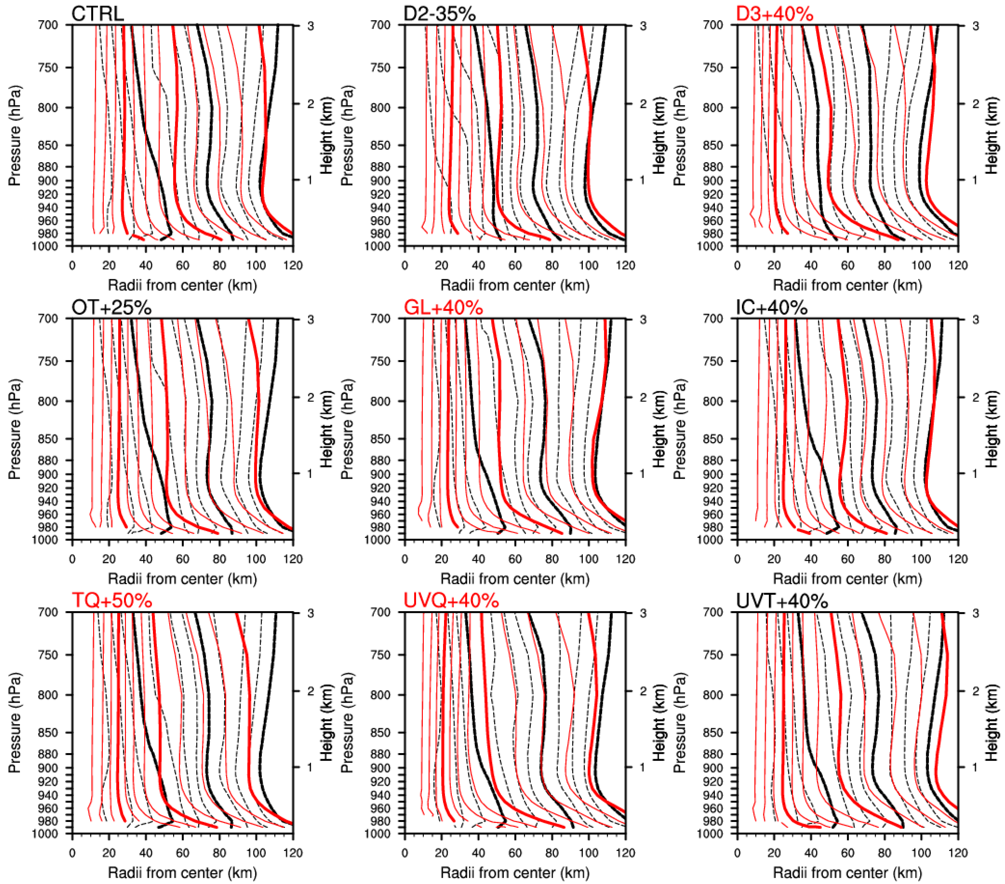
is the Coriolis parameter), in the boundary layer favors for illustrating the evolution of maximum tangential wind. In the boundary layer where absolute angular momentum is not materially conserved, an increase of the absolute angular momentum as decreasing radius indicates a significant increase in tangential wind. It is shown in
Figure 6 that, for the nine ensemble forecast members, the azimuthally averaged absolute angular momentum isopleths have similar distributions. Specifically, the isopleths of assigned value 1.6 × 10
6 m
2 s
−1 at 06 UTC Sept. 26 are generally outside a radius of 60 km from the TC center despite those below 1 km tend to converge inwards. During the following 18 h (i.e., from 09 UTC Sept. 26 to 00 UTC Sept. 27), almost all of the contours move inwards in the lower troposphere; especially, the isopleths of assigned value 1.6 × 10
6 m
2 s
−1 locate inside the radius of 60 km above the height of 500 m, indicating unanimous tendencies of absolute angular momentum convergence. However, the absolute angular momentum convergences exhibit obvious differences between the members reproducing RI and those not. The isopleths of 1.6 × 10
6 m
2 s
−1 show a greater inward displacement over the 06 UTC Sept. 26 –00 UTC Sept. 27 period for the forecast members reproducing RI (i.e., D3 + 40%, GL + 40%, TQ + 50%, and UVQ + 40%), which indicates stronger absolute angular momentum convergences in the boundary layer in these forecast members. Correspondingly, the tangential winds speed up more rapidly and develop to larger values in the forecast members with RI than those without RI (see
Figure 5). Therefore, strong convergence of absolute angular momentum in the boundary layer can raises the possibility of increase the maximum tangential winds and spinning up the inner-core, which is in accordance with the results in Smith et al. [
28], and then favors the onset of RI of TCs.
5.2. Thermodynamics
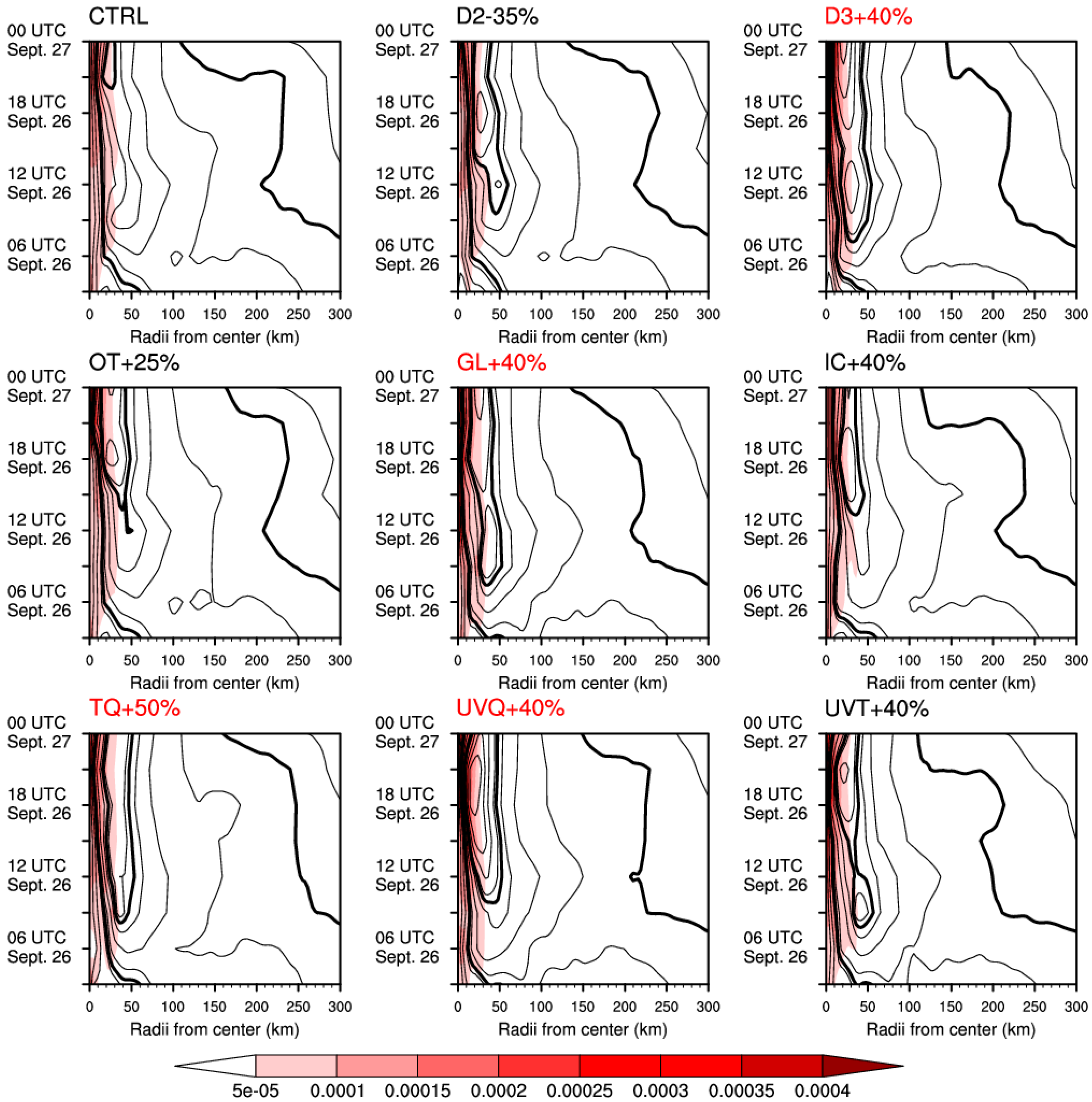
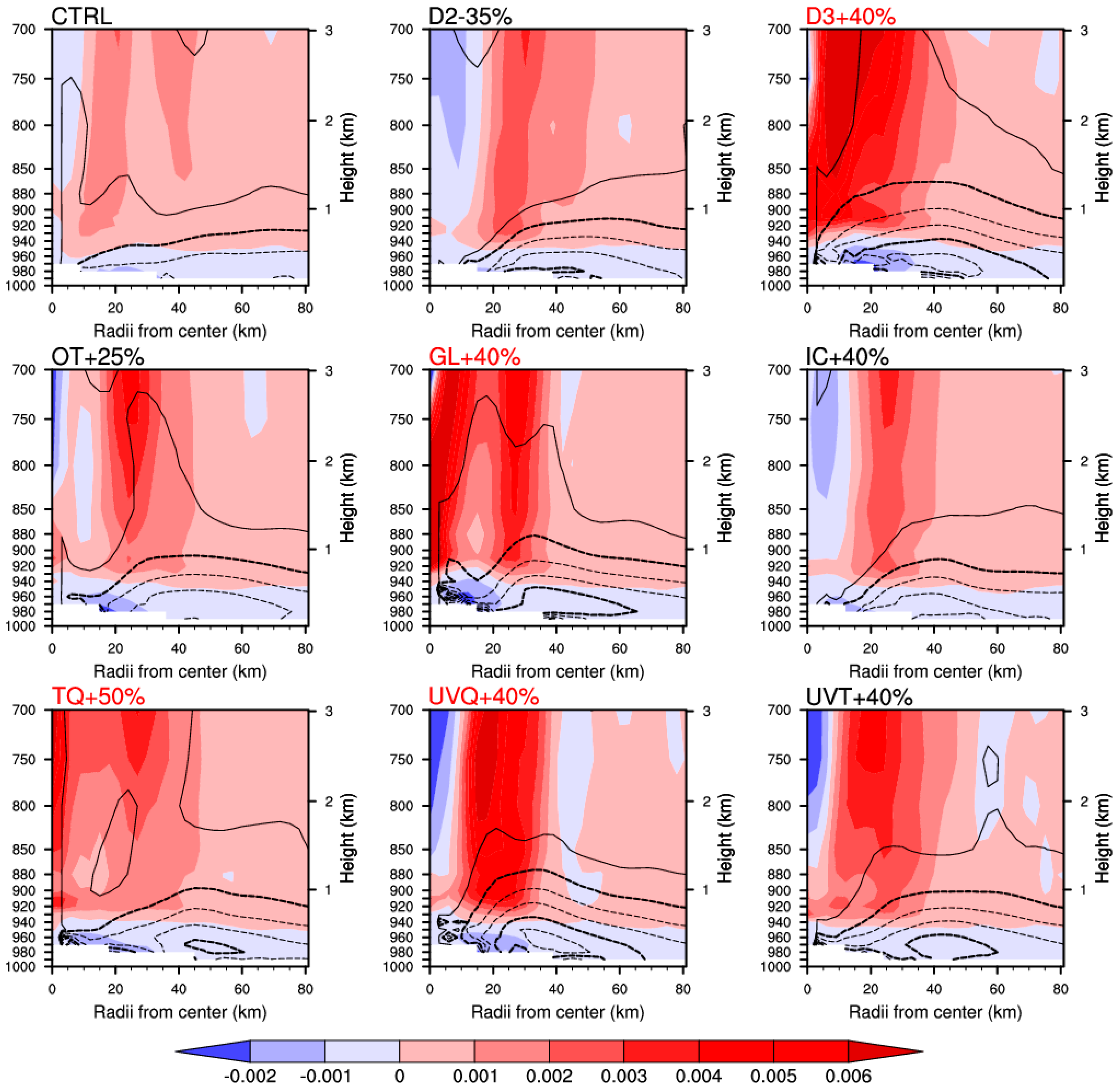
A Hovmöller diagram of latent heating inside a radius of 80 km in the nine forecast members is plotted in
Figure 7. It is shown that, shortly after 06 UTC Sept. 26, latent heating centers is maximized in an annulus between 20 km and 40 km from the centers around 910 hPa, especially in the ensemble forecast members reproducing RI. Moreover, it is noted that the latent heating centers are often located inside the maximum vertical velocity (see
Figure 7) and above the strong inflows. This indicates that the water vapors delivered by the inflow in the boundary layer begin to move upwards and condense much earlier, compared with that in the forecast members without RI. In addition, such latent heating centers move inwards with time, which is coincident with the evolution of the maximum tangential winds. Taking a time average from 09 UTC Sept. 26 to 00 UTC Sept. 27 (over a total of 15 h; see
Figure 8), it is found that more water vapors are accumulated inside a radius of 40 km in the boundary layer in the forecast members reproducing RI, where the water vapor accumulation is measured by the radial wind times water vapor mixing ratio. These water vapors contribute to the continuous latent heat-releasing for over 15 h above the inflow in these forecast members. Moreover, this heating amplifies the local upward motions and promotes the vortical hot towers in the eyewall [
41], which favors the spin-up of the inner-core as shown in
Figure 5, and then for the onset of RI.
In summary, the perturbations superimposed in the gale area of the TC in the boundary layer, especially those including the moisture component represented by the water vapor mixing ratio, enhance the inward absolute angular momentum convergence in the boundary layer, which accelerates the tangential winds. Simultaneously, more water vapor induced by the moisture perturbation is delivered inwards more rapidly by the inflows, which releases substantial amounts of heat around the locations with the maximum tangential winds and contributes significantly to the enhancement of the vorticity inside the inner-core. Consequently, the inner-core spins up rapidly and then RI occurs as shown in the forecast members D3 + 40%, GL + 40%, TQ + 50%, and UVQ + 40%. In contrast, when the perturbations are not superimposed in the gale area or the moisture perturbation is not included as shown in the forecast members without RI, the increase of either the maximum tangential winds in the boundary layer or the vorticity in the inner-core are slower and weaker, both having negative effects on the spin-up of the inner-core, and then RI fails to occur.
6. Summary and Discussions
RI forecasting remains a major challenge in TC intensity forecasting. To investigate the sensitivity of TC intensity forecasts, especially RI forecasts, to the uncertainty occurring in the boundary layer, a variety of ensemble forecast experiments are conducted for Typhoon Dujuan (201521) by superimposing perturbations on the outputs from the YSU scheme. The results show that the track of Typhoon Dujuan (201521) shows a weak sensitivity to the uncertainties occurring in the boundary layer. However, the uncertainty occurring in the TC area in the boundary layer, in contrast with the outer areas, leads to a much larger forecast uncertainty of the TC intensity. In particular, the uncertainty occurring in the gale area of the TC makes a greater contribution to the forecast uncertainty than that in the inner-core and other areas. Moreover, it is found that the uncertainty associated with the moisture in the gale area in the boundary layer of Typhoon Dujuan (201521) contributes most to the RI forecast.
Comparisons between the ensemble forecast members that reproduce the RI and those do not illustrate how the perturbations, especially those with the water vapor mixing ratio component superimposed in the gale area of the TC, offset the errors in the YSU scheme and reproduce RI as reality. Such particular perturbations induce more absolute angular momentum convergences in the boundary layer and latent heat in the eyewall, which favor the increase of the maximum tangential winds and vorticity in the inner-core. Finally, the inner-core is spun up, and RI occurs.
It is known that the uncertainty occurring in the TC area, especially in the gale area in the boundary layer, considerably disturbs the RI forecast accuracy; conversely, it is also the perturbations superimposed on the gale area of the TC that are likely to offset the errors coming from the boundary layer parameterization scheme and help improve the RI forecast skill. Hence, the boundary layer parameterization scheme should be further advanced. Observations can be helpful for optimizing the boundary layer parameterization scheme. It is shown that the forecast uncertainty of the TC intensity is most sensitive to the uncertainty associated with the moisture in the gale area in the boundary layer of Typhoon Dujuan (201521). It is therefore inferred that if sufficient observations, especially those associated with moisture in the gale area within the boundary layer of a TC, can be preferentially implemented, the forecast skill of TC intensity and its RI could be obviously improved.
Zhang and Chen [
42] indicated the importance of the warm upper-level core in the RI of a TC. Qin et al. [
43] showed that the potential temperature variation in the inner-core in the lower and middle troposphere influences the change in the intensity of the TC. In addition, the symmetry of inner-core convection is considered a predictor and can improve the TC intensity forecast skill [
44]. Then this study focused on the thin boundary layer of the TC and emphasized the importance of the gale area in the RI process of the TC by using the WRF with the YSU scheme.
Whether the behavior of the YSU scheme can completely represent the response of the boundary layer is also debatable. Compared to other parameterization processes in the WRF model with several available scheme options, the YSU scheme is the only one relevant to the boundary layer and has been popularly utilized in many studies. Hence, it is a qualified scheme that can generally describe the processes in the boundary layer. It is believed that the results obtained in the present study are instructive. In addition, the uncertainty in other parameterizations schemes as microphysics [
45] and multiscale processes [
46] also significantly contribute to the forecast uncertainty of TC intensity but is out of the theme of this study.


