Article

Spatio-Temporal Variation of Ozone Concentrations and Ozone Uptake Conditions in Forests in Western Germany

1
Department of Geobotany, University of Trier, 54296 Trier, Germany
2
Deutsche Gesellschaft für Internationale Zusammenarbeit (GIZ) GmbH, D-53113 Bonn, Germany
*
Author to whom correspondence should be addressed.
Atmosphere 2020, 11(11), 1261; https://doi.org/10.3390/atmos11111261
Submission received: 8 October 2020 / Revised: 5 November 2020 / Accepted: 17 November 2020 / Published: 23 November 2020

Abstract

:
The study analyzes the long-term trends (1998–2019) of concentrations of the air pollutants ozone (O3) and nitrogen oxides (NOx) as well as meteorological conditions at forest sites in German midrange mountains to evaluate changes in O3 uptake conditions for trees over time at a plot scale. O3 concentrations did not show significant trends over the course of 22 years, unlike NO2 and NO, whose concentrations decreased significantly since the end of the 1990s. Temporal analyses of meteorological parameters found increasing global radiation at all sites and decreasing precipitation, vapor pressure deficit (VPD), and wind speed at most sites (temperature did not show any trend). A principal component analysis revealed strong correlations between O3 concentrations and global radiation, VPD, and temperature. Examination of the atmospheric water balance, a key parameter for O3 uptake, identified some unusually hot and dry years (2003, 2011, 2018, and 2019). With the help of a soil water model, periods of plant water stress were detected. These periods were often in synchrony with periods of elevated daytime O3 concentrations and usually occurred in mid and late summer, but occasionally also in spring and early summer. This suggests that drought protects forests against O3 uptake and that, in humid years with moderate O3 concentrations, the O3 flux was higher than in dry years with higher O3 concentrations.

1. Introduction

Tropospheric (i.e., ground-level) O3 is a secondary air pollutant that causes substantial injury to tree, crop and grassland species through visible injury [1,2], changes in plant physiology [3], acceleration of leaf senescence [4], and decreasing growth, productivity, and fitness of forests [5,6,7,8], with possible consequences for the altered carbon sequestration potential of forest ecosystems [9,10].
Primarily, O3 reduces the photosynthesis activity, which inhibits the growth of plants, thus limiting the net primary production [1]. This impact has been well evidenced in studies on (semi-) natural vegetation [11,12,13], crops [14,15,16], forest vegetation [17,18] and numerous shrub species [19].
Tropospheric O3 is formed by interactions between precursors such as nitrogen oxides (NOx) and volatile organic compounds (VOCs) in the presence of sunlight [20,21,22]. These precursors are produced naturally or emitted from anthropogenic activities such as combustion of fossil fuels used for powering vehicles, power plants or industrial complexes, as well as burning of biomass (e.g., in agriculture).
Other meteorological parameters also influence the O3 formation process, such as high temperature, wind speed and low air humidity [23]. Given the importance of NO2 and NO as precursors for the formation of O3, this study has focused on long-term trends of the concentrations of the pollutants O3, and NO2 and NO as O3 precursors at various sites in Western Germany covering the time period 1998–2019.
During the last 60 years, tropospheric O3 has emerged as an air pollution problem of global dimension with respect to its harmful impacts on human health and vegetation [24].
Investigations on O3 concentrations have been carried out worldwide and have shown that annual mean O3 concentrations increased at various European mountain sites [5,25,26,27,28,29], including sites in Germany [29,30]. Between the late 19th century and 1980, O3 background concentrations doubled to about 30–35 ppb in the mid-latitudes of the Northern Hemisphere and since then it has increased by another 5 ppb to 35–40 ppb [24]. The peak O3 values continue to exceed 50 ppb in many countries in Latin America, North America, Europe, and Africa [31]. Current high O3 levels often occur during growing seasons of forest trees, thereby constituting a risk for the vitality and growth of forests [32,33,34,35,36].
To investigate the O3 risk to forests, which is dependent on the O3 reaching the leaf interior of trees through the stomata, it is crucial to assess the stomatal fluxes of O3 into trees [37,38,39]. To quantify this O3 uptake at plot scale, various models have been developed [40,41]. They require as input meteorological data, i.e., irradiation, temperature, VPD (calculated from air temperature and relative air humidity (the relative air humidity is measured as temperature difference from a wet and dry thermometer; psychrometric difference [42])), wind speed and precipitation, as well we O3 concentrations at canopy height and ecophysiological, ecological and structural vegetation parameters (plant phenology, maximum stomatal conductance (gmax), Leaf Area Index (LAI), canopy height, rooting depth, soil water potential or plant available water content) [39].
Changes in soil water availability influence the stomata opening width and hence the O3 uptake [43]. Water stress or soil water availability is an important factor for O3 uptake of forest trees. For instance, Lin et al. (2020) [44], Gao et al. (2017) [45], Hoshika et al. (2013) [46], Emberson et al. (2013) [47], Gerosa et al. (2009) [48], Matyssek et al. (2006) [49], and Tingey and Hogsett (1985) [50] showed that water stress protects plants from negative O3 effects by closing stomata, hence reducing the O3 flux into leaves. In many parts of the world, including Germany, high levels of O3 concentration often coincide with periods of water stress, e.g., in the exceptional dry year of 2003 [51]. A good indicator also used in this study to describe water stress or arid climate conditions is the atmospheric water balance (AWB), i.e., the difference between precipitation and the potential evapotranspiration (PET) [52]. Using AWB, Prăvălie et al. (2019) [53], Haferkorn (2000) [54], Häckel (2016) [55], and Kasperska-Wolowicz and Labedeki (2006) [52] separated humid, arid and average years varying randomly in time series. AWB also signaled increasing aridity in various countries such as Spain, Italy, and Greece [56,57,58,59].
Changes in precipitation (P), evapotranspiration (ET) and subsequently AWB are imminent effects of climate warming [53].
The present paper is the first paper in a sequence of papers aiming at assessing the risks O3 and climate pose on the health and growth of forests in Rhineland-Palatinate—as an example for a densely forested region in central Europe—and hence its functioning as a source of revenue for the forestry sector. This paper tested the following three hypotheses:
  • The temporal variance of a time series of 22 years (1998 to 2019) of meteorological parameters and air pollutants at five German forest sites corresponds with the global climatic change and air pollution abatement measures implemented during that time frame.
  • The altitude of forest sites and their distance to urban agglomerations as well as the oncoming flow of pollutants (long-range transport of O3 and its precursor substances) and the existence of gaseous reducing agents determine the prevalent O3 concentrations.
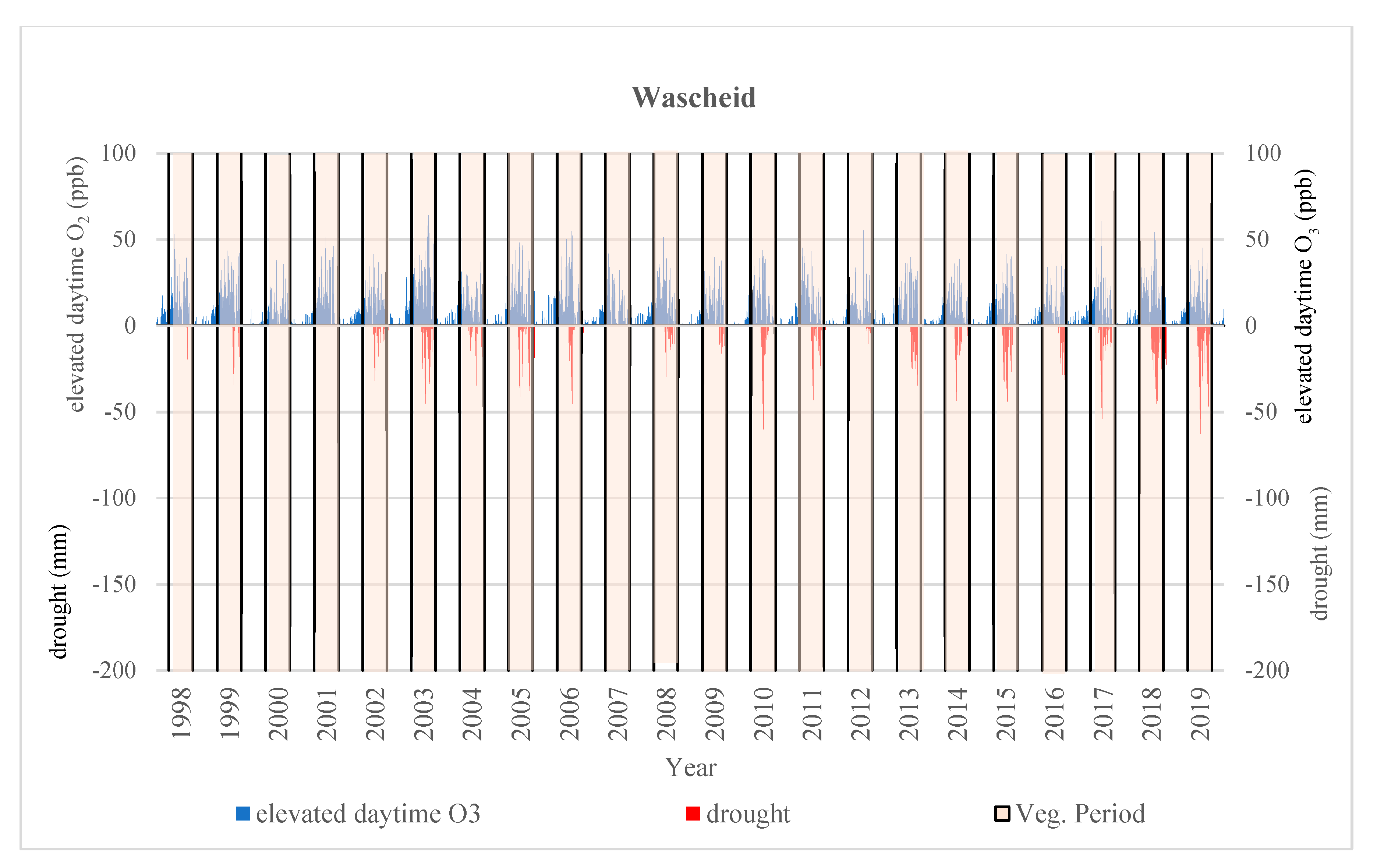
  • The duration, sequence, and intensity of droughts as well as its synchrony with elevated daytime O3 concentrations typical for Central Europe—especially in the montane belt—determine the exposure of forests to O3 and hence influence the trees’ toxicological defense.

2. Materials and Methods
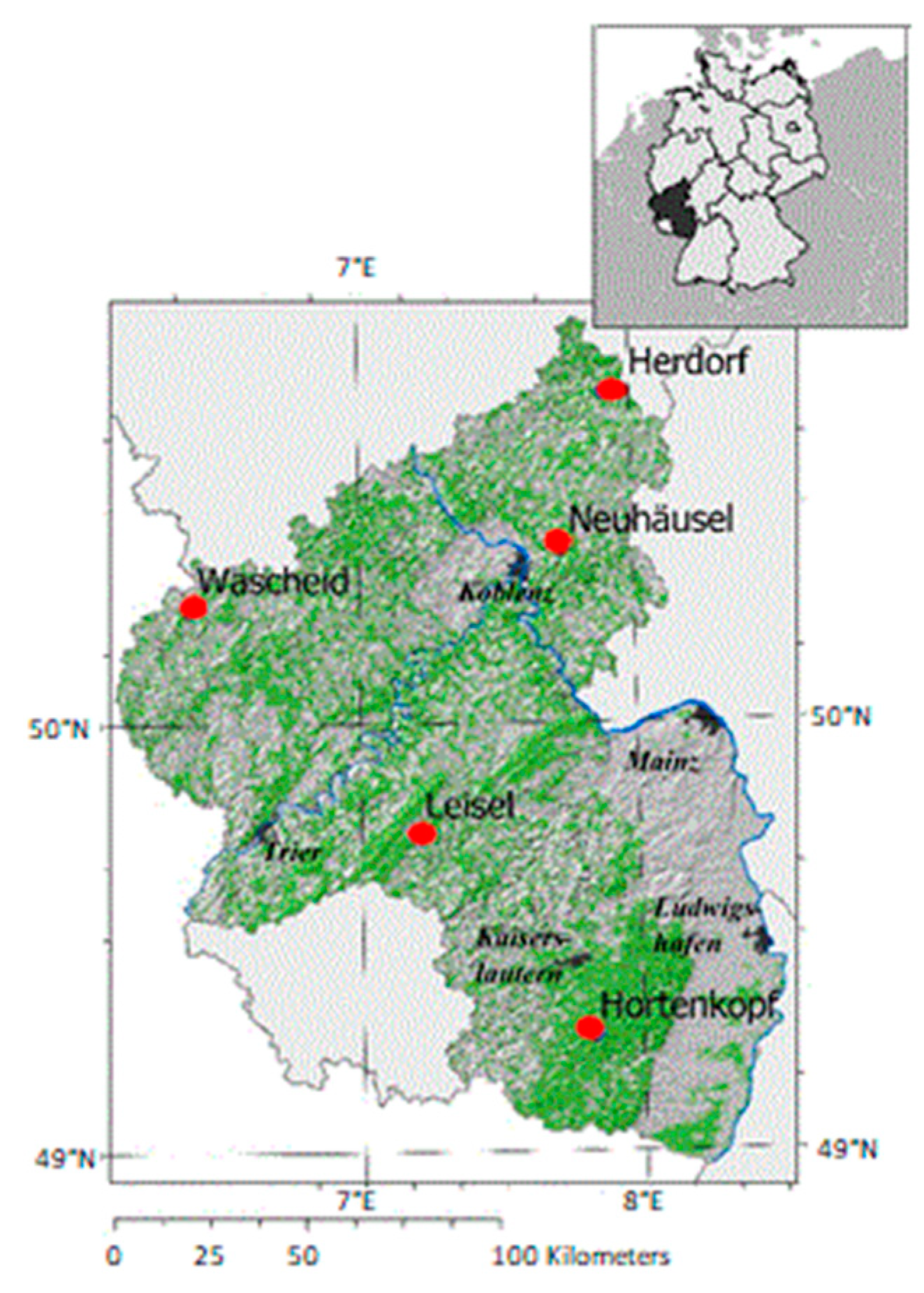
2.1. Study Sites

The study was carried out at five midrange mountain forest sites (Hortenkopf, Neuhäusel, Herdorf, Leisel, and Wascheid (Figure 1, Table 1)) in Rhineland-Palatinate, Germany from 1998 to 2019. These forest plots are managed as Level II plots according to the International Co-operative Program (ICP) Forest [59]. Pollutant concentrations and meteorological parameters are measured at open-field monitoring stations (ZIMEN Stations) close to the forest sites (for distance between ZIMEN stations and forests plots see Table 1). These ZIMEN stations are run by the Environmental Agency of Rhineland-Palatinate on behalf of the Ministry of Environment, Agriculture, Food, Viticulture and Forestry since 1978 (www.luft-rlp.de) [60]. The main task of ZIMEN is to measure the concentration of an array of air pollutants and meteorological parameters.

2.2. Measurements

Each ZIMEN station [60] is equipped with air pollution inlet devices that are mounted on the roof of a container at 3 m above the ground. Pollutants and meteorological parameters are measured continuously (reporting interval of 1 h) with devices listed in Table 2.
Precursor substances like non methane volatile organic compounds (NMVOCs) and methane were not included into the study, because they were only available for the entire time series at the site Hortenkopf. CO was not detectable at the forest plots listed in Table 1.
Plausibility studies [61,62] and comparisons of data with other surrounding meteorological sites revealed deviations especially in precipitation from data collected at ZIMEN stations. So Intermet Data, i.e., interpolated meteorological data from all available climate stations in a raster of 1 km around the Level II Forest Plots (1 km2 raster data), were used to characterize the meteorological parameters T, rH, P and G [63] (Table 2). G, T, VPD, and precipitation were recorded at or calculated for standard height (3 m). Wind speed was measured at 10 m height at the ZIMEN station [60] (see Table 2).

2.3. Methods of Data Analysis

2.3.1. Dataset Quality Assessment

Missing data is a ubiquitous problem in evaluating long-term experimental measurements due to equipment failures, system maintenance, power-failure, and lightning strikes [64]. In the present study, the Intermet Data are free from gaps, because they are interpolated from different surrounding stations. O3 and NOx-Data had data gaps of less than 8% because of data losses during calibration procedures. Data gaps of less than five hours were filled by calculating running averages, while gaps of more than five hours were filled using regression equations for hourly data between the five sites for each year [62,65,66].
The atmospheric water balance (AWB; mm) [55] was calculated to compare different sites in cases of different precipitation and potential evapotranspiration conditions, characterization of similarities (by macro weather situation) or differences in weather conditions (modified by altitude and spatial distribution of the sites) as well as climatic differences in the investigated time series. AWB refers to the difference between the sum of precipitation (P) and potential evapotranspiration (PET; see Equation (1)) [52] and is calculated from daily meteorological data according to the Penman-Monteith equation [67]. To attain daily PET values, we used the output of the DO3SE model Version 3.1.0 [68] (www.sei.org/projects-and-tools/tools/do3se-deposition-ozone-stomatal-exchange/) which is calculated based on Penman–Monteith [67].
AWB = P PET
The AWB only defines the atmospheric aridity and does not consider the whole water supply of plants. A dry atmosphere will lead to higher transpiration demand of plants, which could be balanced to some extent by increased soil water uptake particularly during the night. Only if the plant available soil water (PAW; mm) is limited too, a genuine drought for plants is manifested and can lead to water stress. Such drought is defined in the present study as a day with negative AWB and simultaneously low PAW stock of equal or less than 50% of usable field capacity (uFC (mm)) (see Equation (2)), which is the difference of the field capacity (FC) and permanent wilting point (PWP).
Drought   ( mm ) = Sum   of   daily   negative   AWB   if   PAW < 50 %   of   uFC
A drought affects stomatal leaf conductivity. Hence it is important to estimate the plant available soil water. According to DO3SE [69] and FO3REST [70] models, leaf conductivity would be restricted if the PAW pool declines to less than 50% of uFC. Therefore, the uFC of the appropriate soils were assessed. The uFC assessment was based on soil profile descriptions provided by Landesforsten Rheinland-Pfalz [71], which consider soil texture, soil depth, soil density and stone volume, and then used for calculation of uFC according to the method of Bodenkundliche Kartieranleitung (2005) [72] for the five studied forest plots. To evaluate the daily amount of PAW, the soil water model of FO3REST [70] was applied to calculate the daily change of PAW stock depending on precipitation and evaporation. The model requires detailed (in daily resolution) meteorological parameters of global radiation, the amount of precipitation, temperature, air humidity, and wind speed [69,70]. If this coincides with a negative atmospheric water balance, plants will be exposed to water stress. Periods with restricted negative AWB and smaller than 50% uFC will be accumulated, still surplus precipitation will fill up PAW over a threshold of 50% of uFC. Such defined drought periods will have a length (in days), a frequency within a year and an amount (the accumulation of missing water within a period measured in mm). The amount, duration, day of the first appearance, and the frequency of drought during a vegetation period will be used to characterize yearly drought or water stress periods of a sites. This provides a way to compare different sites and characterize the weather conditions with regard to gas exchange conditions much better as the correlation to measured meteorological parameters, because the atmospheric water conditions are extended by available soil water conditions.
Furthermore, mean daytime O3 concentrations (mean daytime O3 is the daily mean of hourly O3 concentration if the global radiation is higher than 50 W/m2; following the AOT40 definition) were calculated. The mean daily daytime O3 concentration of the entire period from 1998–2019 was subtracted from each daily mean O3 concentration to define elevated daily O3-concentrations if they were higher than zero (Table S1).
Lastly, the synchrony or asynchrony of elevated O3 concentrations and drought periods was examined as this enables a qualitative view on the O3 uptake risk, i.e., to identify days with high, medium, and low potential O3 uptake rates. Asynchronous days will have a higher O3 uptake risk, because leaf conductivity will not be restricted by water stress, whereas synchronous days of elevated O3 concentration and drought will lead to reduced or entire stomata closure, which protects the trees against O3 uptake.

2.3.2. Statistical Methods for Spatial and Temporal Data Analysis

Statistical analyses were done with Excel, SPSS, and R. The temporal trend in air pollution and meteorological data were calculated with regression analysis of annual means against the years. Scheffé’s test was used as location test after the application of an ANOVA to check whether there were significant differences between sites measuring O3 and NO2 parameters over 12 months (Table S2).
Moreover, to identify correlations between all parameters, which will influence O3 concentration and leaf conductivity, a principal component analysis (PCA) was applied to identify the importance of the variables in each factor [73,74,75,76,77,78,79,80]. This method is concerned with identifying linear components within datasets and with how a particular variable might contribute to that specific component. PCA interpretation depends on understanding eigenvalues and eigenvectors. Eigenvalues are the coefficients attached to eigenvectors, which give the axes magnitude [81,82,83,84,85].

3. Results

3.1. Temporal, Spatial Variance and Correlations of Pollution and Meteorological Data

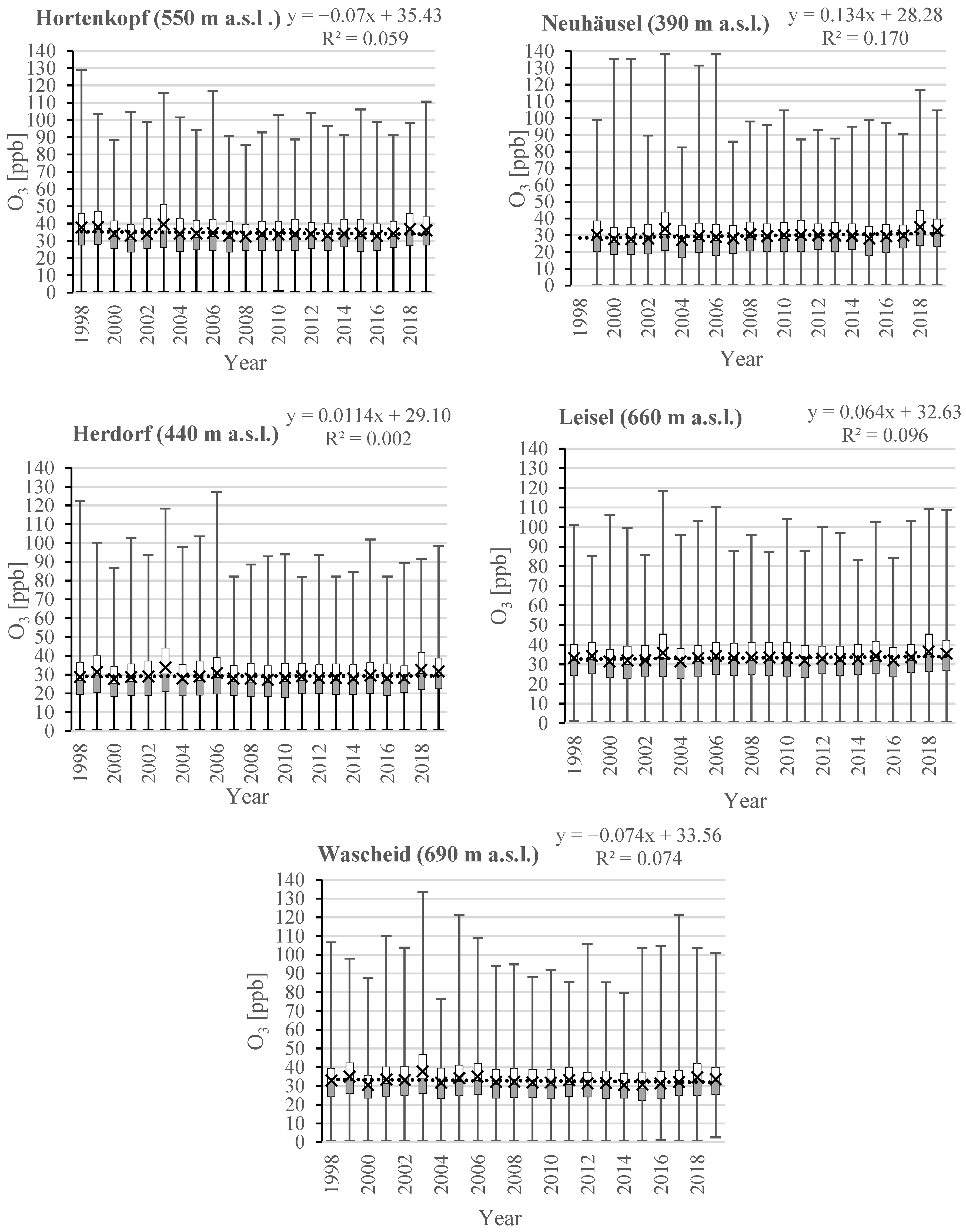
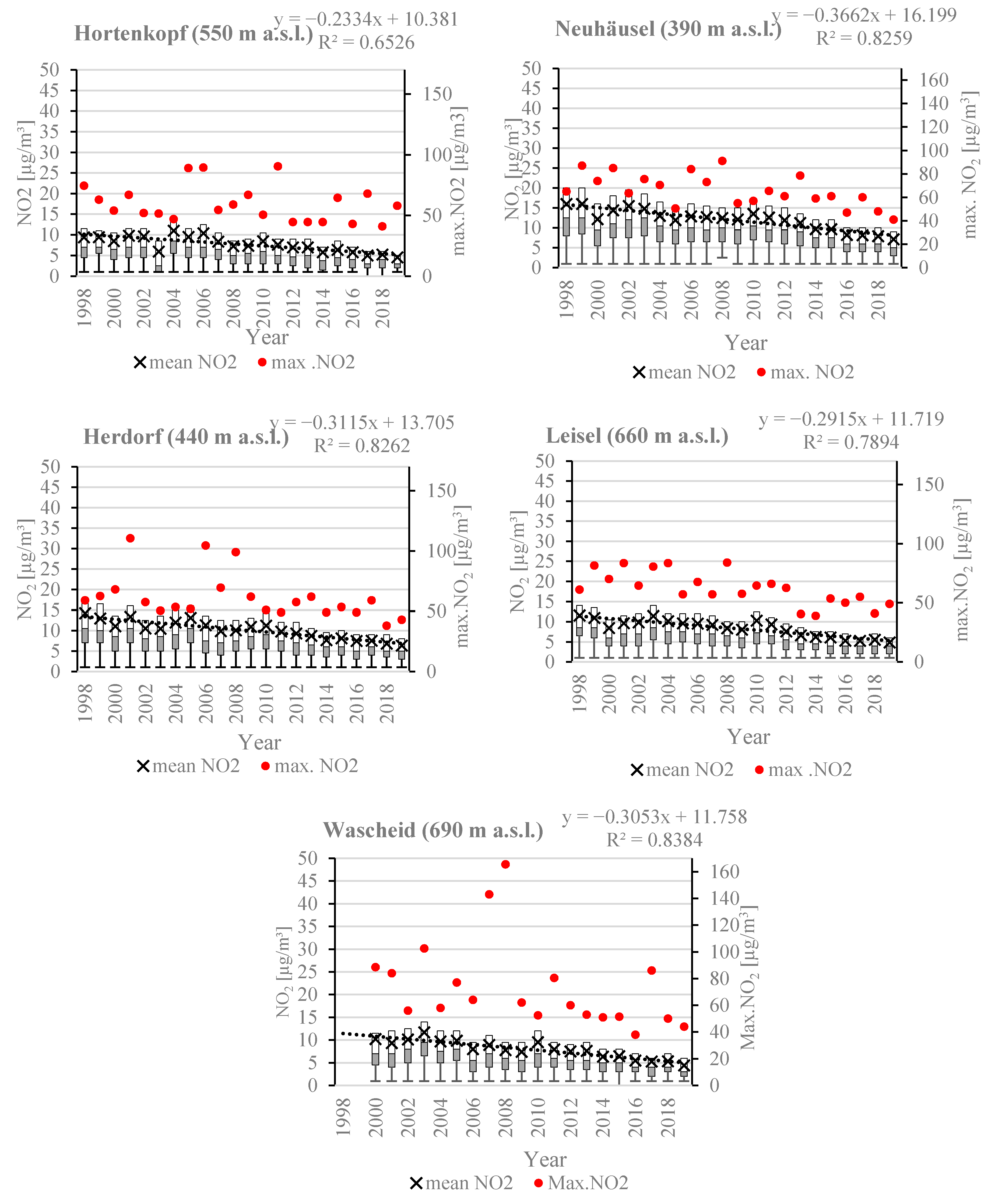
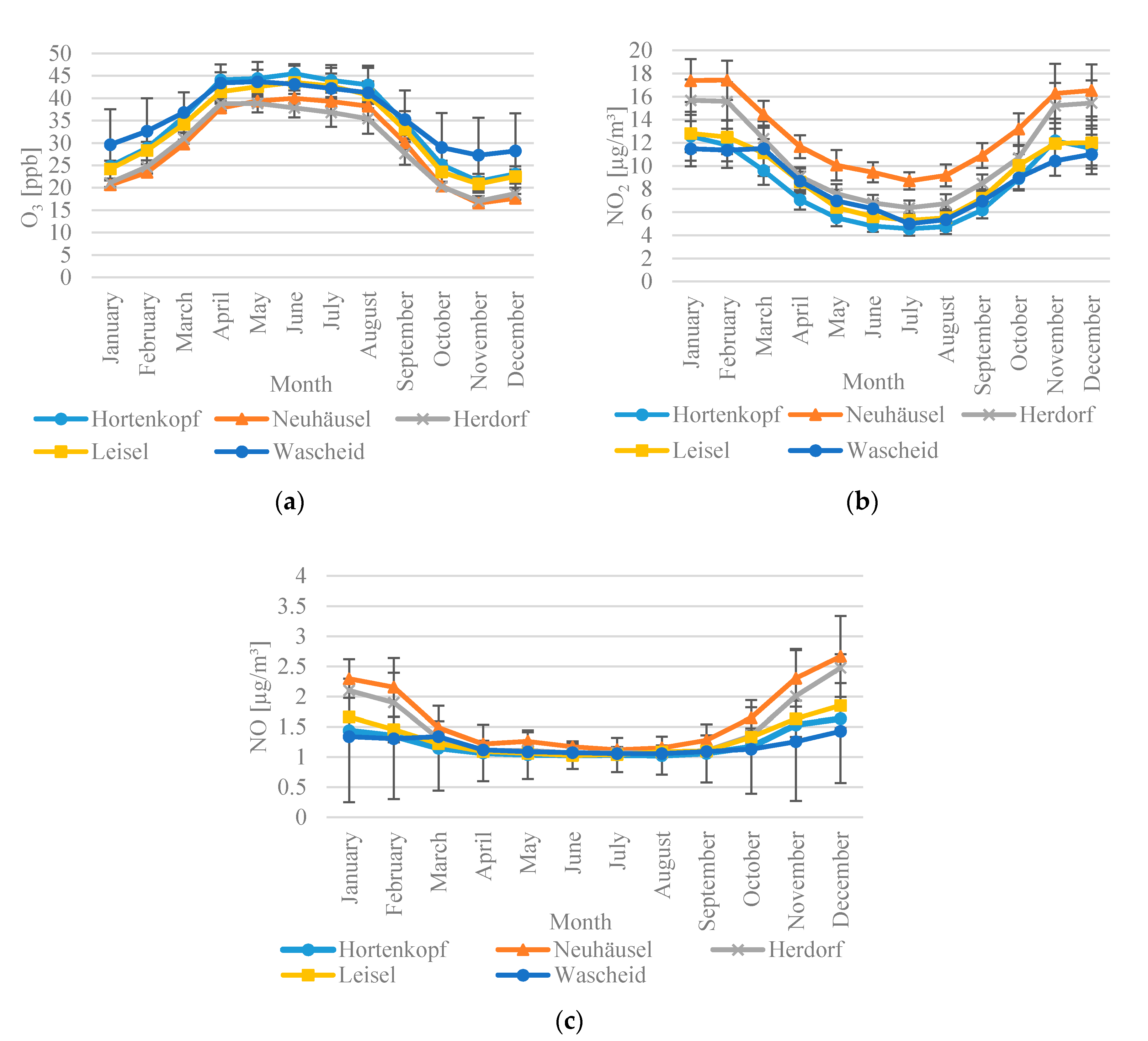
3.1.1. Temporal Trends

The boxplots (Figure 2) illustrate the annual range of hourly O3 time series data at all five sites for the years 1998–2019, except for Neuhäusel in 1998, when it experienced a large data gap. These boxplots show the quartiles and medians of O3 concentration displaying the annual variation of the particular data set.
The annual mean O3 concentrations of the sites ranged from 27 to 40 ppb (Table S1). Hortenkopf showed the highest annual mean of O3 concentrations (32 to 40 ppb) in every year (except 2008 when Leisel showed the highest annual mean). On the other hand, two sites of lower altitude (Neuhäusel and Herdorf) exhibited the lowest annual mean of O3 concentration (27 to 34 ppb) in every year. The hourly maximum of O3 did not exceed 138 ppb at all sites and the maximum annual mean O3 concentration was found at all sites in 2003 (Figure 2). At all sites, the O3 concentrations did not show a significant trend during the 22-year study period (Table 3).
At all sites, the annual mean of NO2 concentrations ranged from 4.5 µg/m3 to 16 µg/m3, with Neuhäusel and Herdorf showing the highest annual mean (16 µg/m3 and 14.2 µg/m3, respectively) in every year. The hourly maximum of NO2 was less than 175 µg/m3 at all sites. However, there were significant spatial discrepancies among the sites (Table S2).
Boxplots of NO2 concentrations will display unproportional long whiskers of the 4th quartiles and therefore the maximum values which limits the 4th quartile are displayed as points on the secondary y-axis in Figure 3. This unusual change highlights the temporal trend over the whole time series. The unproportional long 4th quartile indicates the skewed distribution of NO2 concentrations with dominating low hourly concentrations (smaller than 15 µg/m3; 1st to 3rd quartile) in comparison to the 4th quartile which are spread over a longer concentration range. This points out that extremely high NO2 concentrations of the 4th quartile are rare events, but they should not be marked as outliers, because they are plausible measurements attributed to presumably nearby combustion events or transport processes.
The annual mean concentration of NO2 and NO (around 2 µg/m3), despite high variances (Figure S1), presented an overall significant decreasing trend since the end of the 1990s (Table 3). In addition, the extreme values show the same trends with exception of NO, where the lowermost values are frequently smaller or equal than 1 µg/m3.
None of the sites (with exception of Herdorf) showed significant increasing trends in temperature, while global radiation increased at all sites inclusive the peak values (Table 3). At all sites, peak values of precipitation and wind speed (except Leisel) decreased with exception of Neuhäusel and Leisel (Table 3). The temporal increase of global radiation included the peak values (Table 3). Only at Hortenkopf and Herdorf an increase of VPD peak values is significant.
Very important is that mean O3 (24 h and daytime) concentrations do not show any temporal trend. They vary around the same level for the duration of the whole time series investigated. Only at Hortenkopf an increase of peak values was assessed, whereas in Neuhäusel and Herdorf an increase of the lowermost values was significant. These two effects will determine a steady mean value of O3 during the time series on a site.

3.1.2. Spatiotemporal Trends

The typical yearly annual course of O3 and its precursors NO2 and NO is opposite. High O3 concentration levels were present from April to September (Figure 4a). The highest monthly mean O3 concentration value of 45.5 ppb was observed in June at Hortenkopf while the lowest value of 16.6 ppb was found in November at Neuhäusel. The curve progression from the sites Hortenkopf, Leisel and Wascheid (the highest altitude sites) showed nearly the same O3 concentrations from April to September, and only outside the vegetation period in January, February, and March as well as in October, November, and December did they differ. A different curve shape was observed at Neuhäusel and Herdorf with significantly smaller concentrations throughout the whole year. Table S2 shows significant differences between months and sites in two groups with higher altitudes and smaller population density (Leisel, Wascheid, Hortenkopf) on the one hand and lower altitudes with higher urban density on the other hand (Neuhäusel, Herdorf). Herdorf showed the lowest O3 concentrations during the vegetation period of all sites, with the Scheffe’ test approving that there is a significant difference in some months (April and June) during the vegetation period between sites (Table S2).
An opposite temporal course as compared to monthly mean O3 concentrations were found for nitrogen oxides (Figure 4b,c). NO2 and NO concentrations were highest during the wintertime. At Neuhäusel and Herdorf the highest NO and NO2 concentrations were recorded outside the vegetation period from October to March. The lowest NO2 and NO concentrations were observed in the hottest months of June, July, and August. The highest monthly mean NO2 concentration of 17.4 µg/m3 occurred in February at Neuhäusel, whereas the lowest value of 4.6 µg/m3 was found in July at Hortenkopf (Figure 4b). Furthermore, the highest monthly mean NO concentration of 2.67 µg/m3 occurred in December at Neuhäusel, whereas the lowest value of 1.03 µg/m3 was found at Hortenkopf in August (Figure 4c).
Neuhäusel and Herdorf possess the highest values of NO2 while sites at higher altitude like Leisel, Wascheid, Hortenkopf exhibit lower values during the year. The higher NO2 concentrations at the site Neuhäusel differ significantly from the other sites (Table S2).
Neuhäusel and Herdorf showed the highest annual means of NO concentration (2.2 µg/m3 and 2 µg/m3, respectively) in every year and the hourly maximum of NO concentration did not exceed 170 µg/m3 at all sites (Figure S1). The levels of NO2 and NO concentrations of Neuhäusel and Herdorf were higher than those of Hortenkopf, Leisel, and Wascheid.
The spatial distribution of meteorological parameters, as a function of altitude, is shown in (Table S1). For example, higher altitudes experienced lower temperatures and VPD but higher precipitations and O3 concentrations. On the other hand, in low altitude sites, temperature was higher whereas precipitation and O3 were lower than at high altitude sites (Table S1). Moreover, there are significant differences between sites for meteorological parameters during the time series (Figure S2). For example, yearly mean temperatures were significantly lower in Wascheid than at all other sites for every year (Table S1). Wind speed showed (Figure S2) significant differences between all sites (e.g., 1998, 2004, 2011, 2014, 2017, and 2019) and the values were significantly higher in Herdorf in some years.

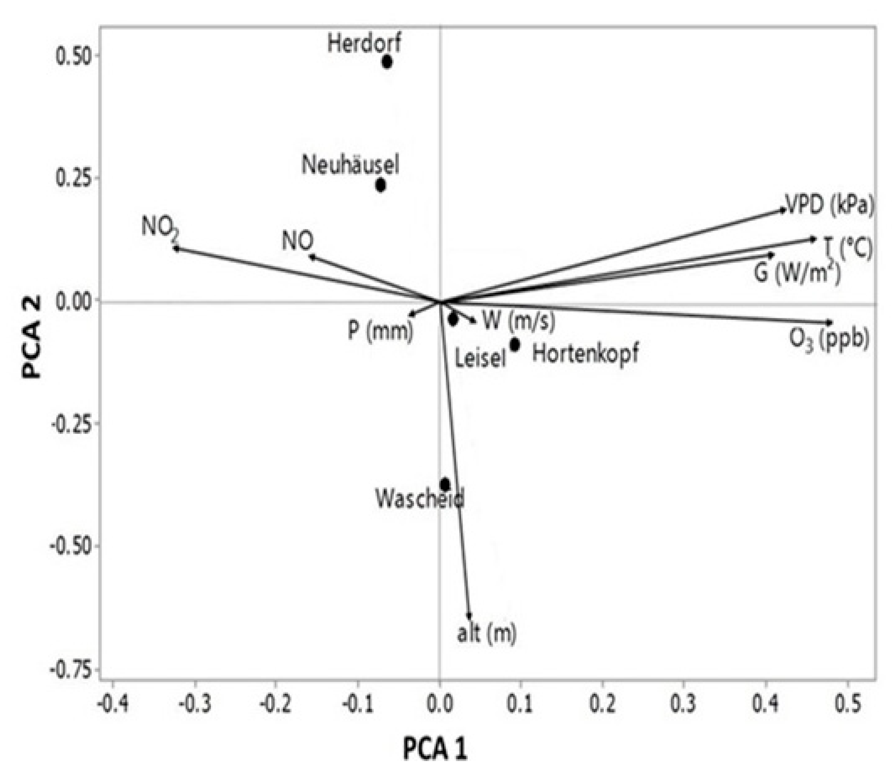
3.1.3. Correlations between the Parameters

To characterize all correlations between all parameters and to identify the main factors contributing to the variance between data, a principal component analysis was performed (Figure 5).
The PCA was performed on meteorological and pollution data in hourly resolution to identify the variables with the most important impact on variance (Figure 5, Table 4 and Table 5). The first and second axes justify the most significant changes in the eigenvalues, respectively, at 3.05 and 2.30, corresponding to 21.8% and 38% of the accumulated variance, respectively (Table 4). The PCA revealed that higher NO and NO2 values were associated with Herdorf and Neuhäusel (Figure 5). NO2 and NO were negatively correlated with O3 concentration, wind speed, altitude, temperature, and global radiation. High altitude and high wind speed values were associated with the sites Hortenkopf, Leisel, and Wascheid (Figure 5).
Accordingly, VPD, T, G, and O3 concentration vectors point in the same direction. The low angle is a sign of the high correlation between these parameters and the first axis. Moreover, there were very long vectors such as VPD, T, G, and O3 that highlight the importance and high contribution of the first axis as compared to vectors with shorter length like P and W with wide angles to both axes. The Pearson correlation coefficients for O3, NO2, NO, and the meteorological parameters are shown in Table S3 for all sites. It shows that O3 concentrations were negatively correlated with NO and NO2 at all sites. Furthermore, there was a positive correlation between NO and NO2 at all sites. O3 features a positive correlation with global radiation, temperature, and VPD while NO2 and NO show a negative correlation with temperature, global radiation, and VPD. Moreover, O3, NO2, and NO had week correlations with wind speed and precipitation at all sites.

3.2. Characterization of Arid Periods as Conditions of Reduced Gas Exchange at the Forest Sites

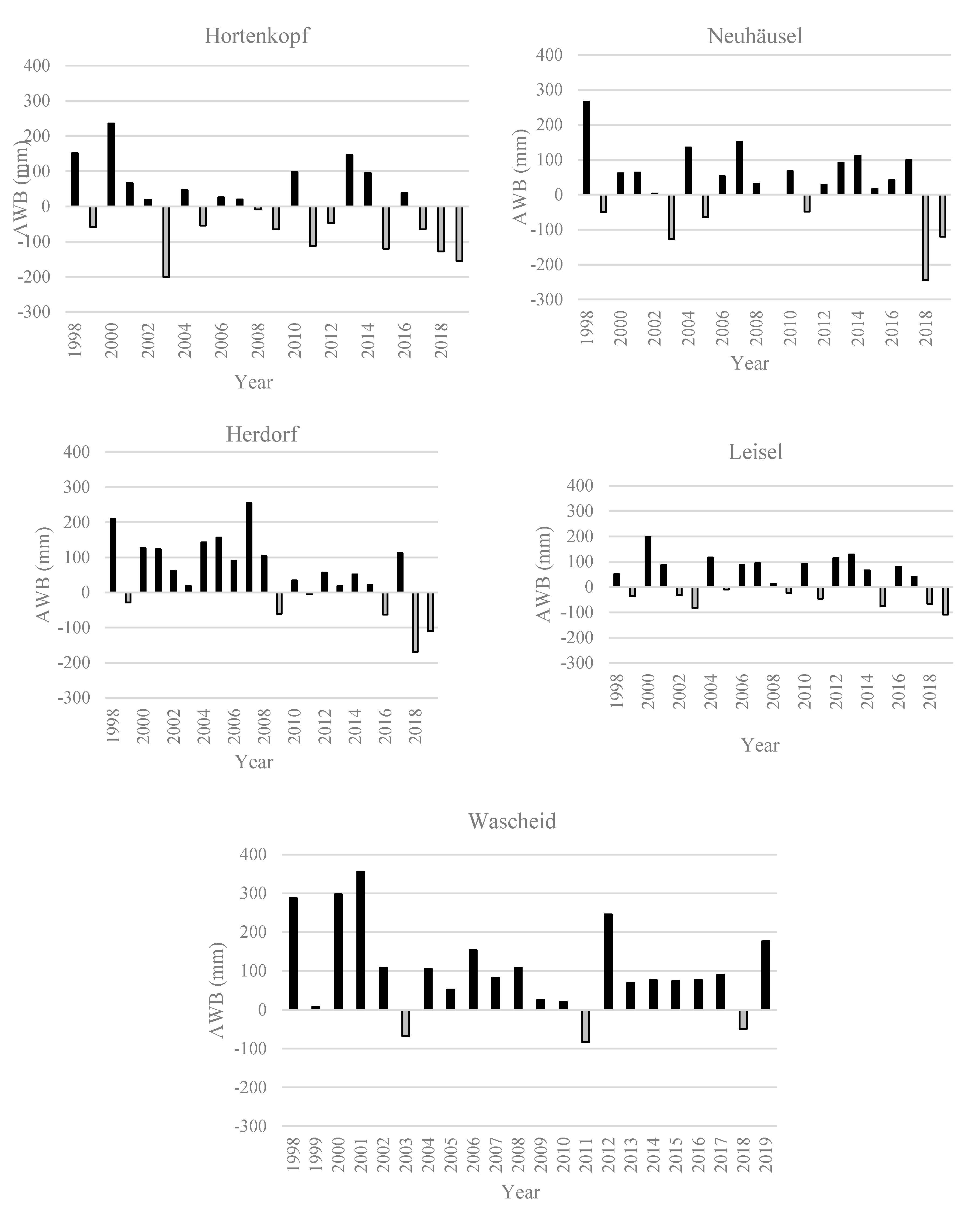
3.2.1. Atmospheric Water Balance

To characterize varying conditions for the exchange of gases (CO2, O3, water vapor etc.) through the trees’ stomata during the investigated time period, it is important to look at the AWB. Figure 6 shows the AWB of the sites during the growing season (1st April to 30th September) of the years 1998 to 2019. Black columns illustrate humid periods with a positive balance (more precipitation than evapotranspiration) while grey columns depict arid periods with more evapotranspiration than precipitation. Hortenkopf (11 periods) and Leisel (nine periods) offer the highest frequency of arid periods. Neuhäusel (five periods), Herdorf (six periods), and Wascheid (three periods) were more humid and showed fewer arid periods over 22 years. With exception of Herdorf, the vegetation period 2003 presents water deficit at all sites. The vegetation periods in 2011, 2018, and 2019 were arid too at all sites with exception of the site of highest altitude and precipitation sum in Wascheid. Humid vegetation periods were present in the investigated time series in 1998, 2000, 2001, 2004, 2007, 2008 (except Hortenkopf), 2013, 2014, 2016 (except Herdorf), and 2017 (except Hortenkopf) at all sites. Figure 6 points out that the highest negative balance values were observed at Neuhäusel (–245 mm, in 2018) in the north-east of Rhineland-Palatinate (Westerwald). In contrast, the highest positive value of AWB (with 356 mm water excess in 2001) was found in Wascheid (north-west of Rhineland-Palatinate, Eifel).

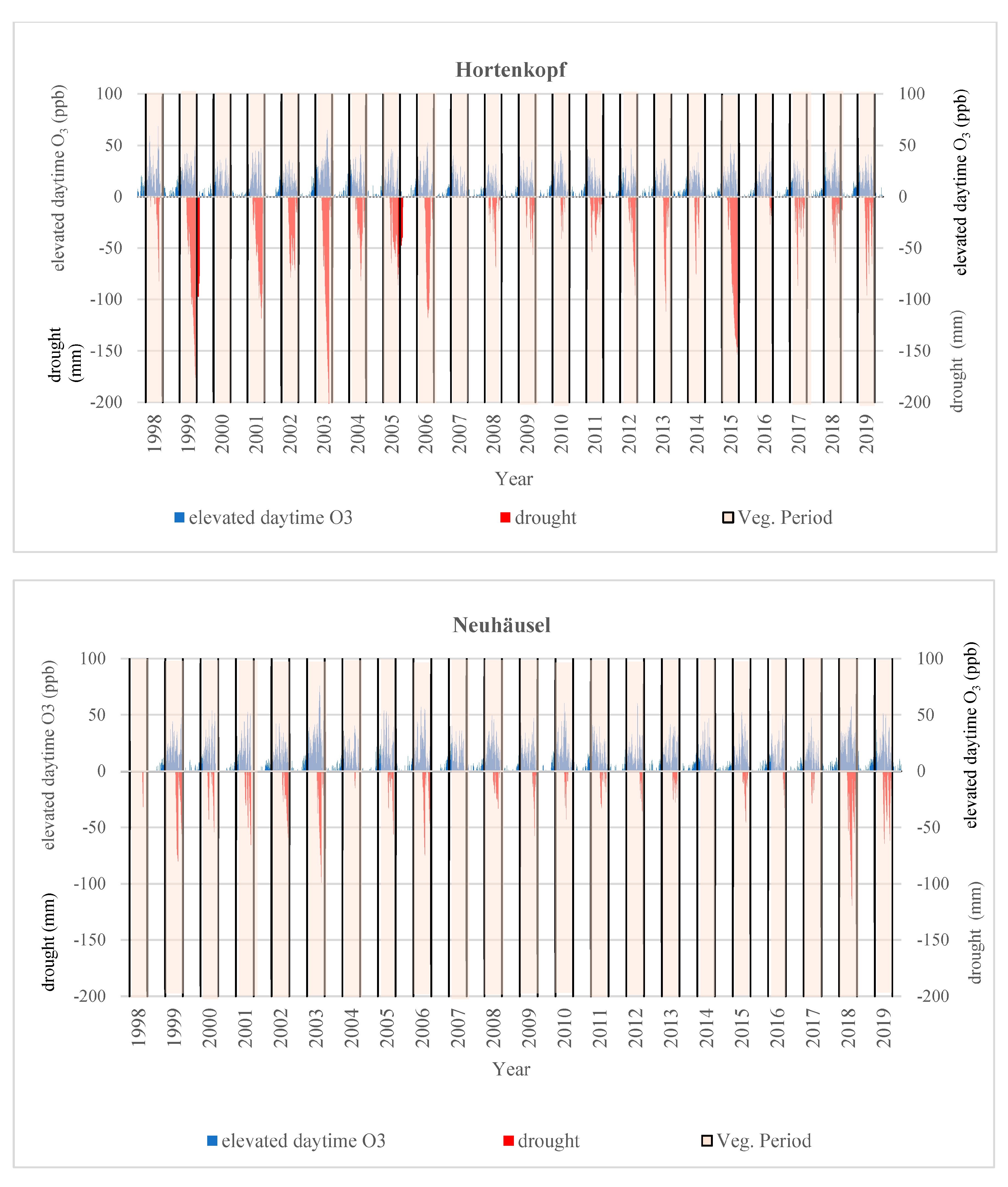
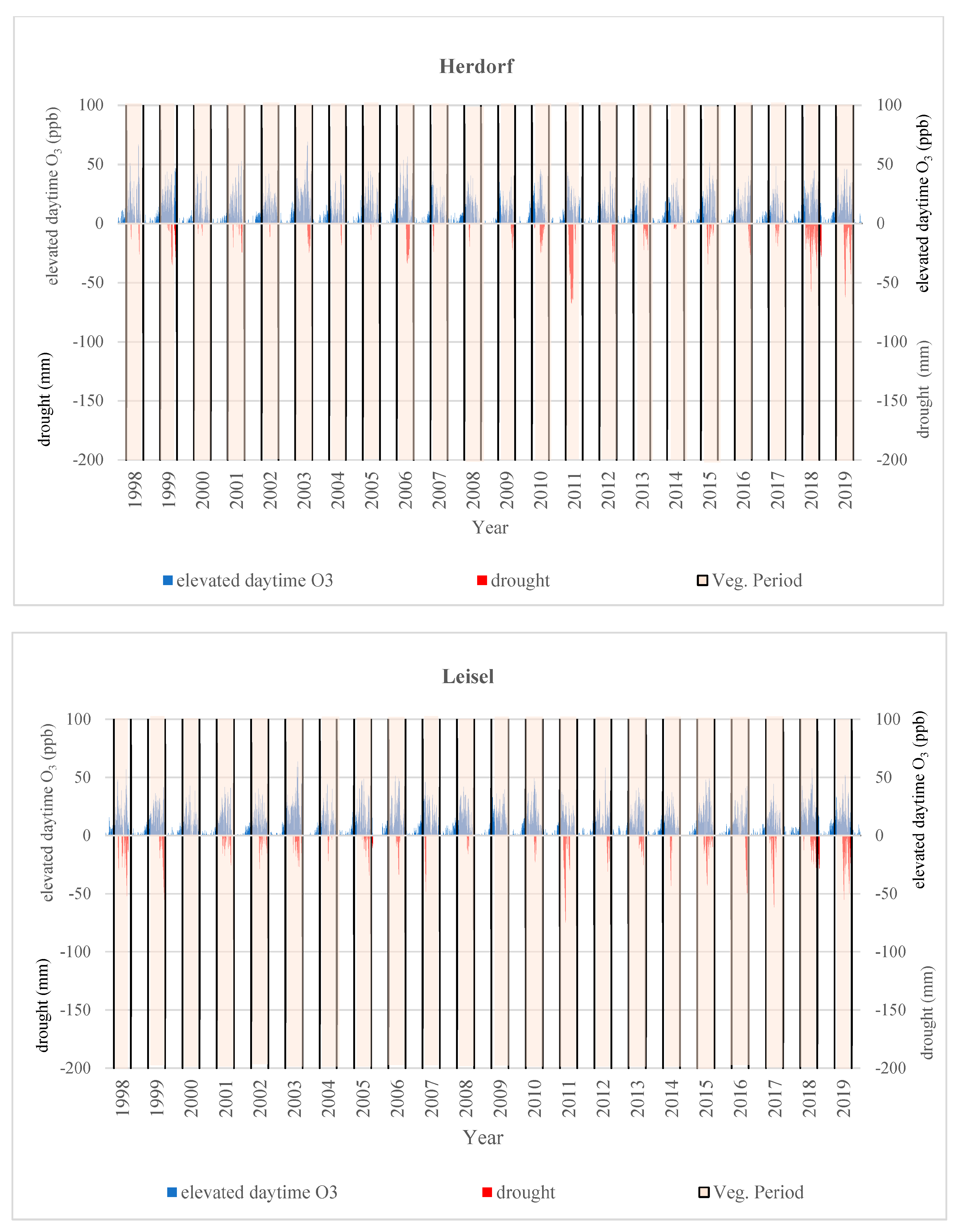
3.2.2. Drought Intensity and Elevated Daytime O3 Concentrations

To characterize drought intensity in the present study, negative AWB values were accumulated during a year, if the water supply in the soil was below 50% of the useable Field Capacity (uFC) (lower part of Figure 7). Negative values of AWB are an indicator for an arid atmosphere. uFC values in the rooting zone of 100 cm at the five forest sites are listed in Table 6. Negative values of AWB, mainly predominantly attributed to evapotranspiration, reduce the supply with plant available water (PAW). According to Table 6, Neuhäusel had the highest while Herdorf and Leisel had the smallest uFC value.
Figure 7 shows the spatio-temporal variability of drought (daily resolution) as the accumulated negative daily AWB and elevated daytime O3 concentrations for each year of the study time series. It demonstrates that during the vegetation period, especially from June to the end of August (153 to 244 DOY), dry weather conditions and elevated daytime O3 concentrations are very frequent at all sites. Generally, drought events are more frequent in mid and at the end of summer and sometimes reach into autumn, when the O3 concentrations start to decrease. Moreover, it displays that the longest drought duration and highest drought intensity were found at Hortenkopf (131 days in 2011 and −204.9 mm in 2003, respectively) (Table S4). The lowest drought intensity and most humid years were observed in 1998, 2000, 2004, 2007 and 2008 without any drought at most sites. Figure 7 shows that Herdorf (site with the highest uFC) was the site with the shortest number of drought days and lowest intensity of accumulated drought during the vegetation period. Sites at higher altitude like Leisel and Wascheid showed less frequency and intensity of drought (with exception of 2003), especially in the years up to 2010. There are only few cases where the drought exceeded the end of the vegetation period (e.g., Hortenkopf 1999 and 2005).
The years 1999, 2003, 2006, 2011, 2015, 2018, and 2019 had the longest drought periods and the highest drought intensity. In 2000 and 2007, hardly any drought periods occurred across all sites. These years can hence be classified as humid years.
Figure 7 also presents elevated daytime O3 concentrations (daily daytime O3 mean with global radiation higher than 50 W/m2 diminished by time series mean of daytime O3 concentration). O3 is also prevalent outside the vegetation period at all sites. However, this is usually of minor threat for forests, because only coniferous trees might take up some O3 during those months (at a much-reduced rate only due to non-favorable gas exchange conditions). Nonetheless, Figure 7 displays the elevated daytime O3 concentrations over the entire year and not only for the vegetation period. A higher frequency and intensity of drought existed during the vegetation period, often in late summer under good O3 formation conditions (high radiation, warm and dry weather conditions) and hence simultaneous elevated daytime O3 concentrations. The year 2003 showed the highest daytime O3 concentrations at all sites (Figure 7 and Table S4).
When qualitatively identifying the synchrony or asynchrony of elevated O3 concentrations and drought periods for the whole time series from 1998 to 2019, Hortenkopf and Herdorf experienced the highest and lowest risk for O3 uptake with 32.8% and 15.8% of asynchronous days, respectively. Conversely, the highest and lowest synchrony between elevated O3 concentrations and drought was found for Leisel with 60.8% and for Hortenkopf with 45.6%, respectively. Hence, Hortenkopf will be the site with highest potential risk of O3 uptake. Periods with no synchrony between elevated O3 and drought, were particularly prevalent during the humid years 2000 and 2007 (see Table S4), having most likely led to high O3 uptake. These qualitative results suggest that O3 fluxes might have been on average higher in relatively humid years as compared to arid years and that there is a distinct correlation between AWB or drought intensity and O3 uptake.

4. Discussion

4.1. Spatial and Temporal Trends of Meteorological and Pollution Data (O3, NO2 and NO)

The analysis of a 22-year long time series of weather and air pollution data recorded at five forest sites in Western Germany revealed differences in air quality and meteorological conditions between these sites, with some of them being significant. These differences can partly be explained by different altitude and distance to human settlements with increased traffic and industrial activity.
The study revealed a clear decreasing trend in NO2 and NO concentrations between 1998 and 2019, which is in agreement with findings by the German Environment Agency (UBA) [86], Junk et al. (2003) [87] and Georgoulias and Stammes (2019) [88]. The sites in the present study located above 500 m a.s.l. (Hortenkopf, Leisel, and Wascheid) are good examples for sites affected by long-range O3 transport, while the lower altitude sites are more affected by local O3 formation due to local precursor emissions [89]. Figure 4b,c show high monthly mean NO2 and NO concentrations during the winter period due to increased emissions from the use of fossil fuels for heating [90,91]. NO2 (17.4 µg/m3) and NO (2.67 µg/m3) concentrations were highest in winter months, possibly reflecting increased residential heating. Junk et al. (2003) [87] stated high monthly NO2 concentrations in winter and low monthly NO2 concentrations in summer in Trier, Germany.
Surprisingly the present study revealed no temporal trend in mean 24 h or daytime O3 concentrations during the time series. It seems that that decreasing O3 extremes (95% Quantile) and increasing low O3 concentrations (5% Quantile) held the high varying O3 concentration on unmodified level (Table 3). High O3 concentrations recorded during the 22 years at some high-altitude sites might be the result of long-range transport from nearby urban agglomerations, as the concentrations of O3 precursors (e.g., nitrogen oxides) at these sites are too low to explain the high O3 concentrations. These precursors are transported into clean air forest regions, where reduction agents in the air are either missing or are rare, hence O3 has a higher life expectancy as in densely populated urban areas. Differences in O3 concentrations depending on different altitudes are not as distinct as expected. That may have two reasons, at first the altitudinal gradient in the present study is small (200–300 m) compared to other studies and second the long-range transport of O3 and the distances of the stations to urban agglomerations could be different to other studies. This is in agreement with Sicard et al. (2009) [27], who reported a slightly increasing trend in tropospheric O3 between 1995 and 2003 at French rural monitoring network stations, which was strongly influenced by the altitude. Also, Klingberg et al. (2009) [92] in Sweden and Wehner and Wiedensohler (2003) [93] in Germany showed that high global radiation at high altitudes is contributing to high O3 concentrations, which supports the findings of the present study. As shown in Figure 2 and Table S1, 2003 was exceptionally hot with the highest global radiation and the highest O3 concentrations as compared to the other years. Baumgarten et al. (2000) [94] and Treffeisen and Hald (2000) [95] argued that the cumulative hourly O3 concentrations were enhanced at higher altitude stations in Germany as compared to lower altitude stations most likely due to transport from urban agglomerations.
Figure 4a shows a higher mean O3 concentration observed in summer as compared to the winter due to high temperature, low humidity and high light intensity, all of which promote O3 formation [96]. Similar annual trends in Germany were observed by Treffeisen and Halder (2000) [95] and Meleux et al. (2007) [97].
Surface O3 showed negative correlations with NO and NO2 at all stations (Table S3). Therefore, a rise in O3 concentrations is associated with a reduction in NO and NO2 concentrations. Correlations among the concentrations of different pollutants (O3, NO2, and NO) were stronger at Herdorf than in other forest stations, because it was the lowest altitude station of this study with a higher density of traffic and human activity. Mavroidis and Ilia (2012) [98], Latif et al. (2014) [99], and Minkos et al. (2020) [86] found corroborating results, i.e., that there is are close correlations between concentrations of different pollutants (O3, NO2 and NO).
Figure 5 and Table S3 show correlations of meteorological parameters (G, VPD, T, P and W) with O3 concentrations, reflecting photochemical processes in the atmosphere which are responsible for O3 formation. Figure 5 illustrates the highest O3 concentrations during periods with low precipitation. Lower precipitation (lower cloud cover) usually corresponds with higher global radiation, higher temperatures, and higher O3 formation rates as reported by Tarasova and Karpetchko (2003) [100] and Kovač-Andrić, et al. (2009) [79]. Dawson et al. (2007) [101] indicated that temperature exerted the largest influence on O3 concentrations. Singla et al. (2012) [102] revealed a strong correlation between global radiation intensity and O3 concentration. The analysis of Camalier et al. (2007) [103] confirmed that O3 increases generally with increasing temperature while O3 decreases with increasing relative humidity (because relative humidity usually decreases with increasing temperature). All these investigations confirm the results obtained by this study, which showed that in higher altitudes the air is cooler and more humid, and the vegetation periods are shorter, thereby representing a montane climate. Furthermore, the VPD is lower but wind speed is higher as compared to lower altitudes (Table S1).
The present investigations also display increasing temporal trends in global radiation at all sites probably as result of less cloud cover, decreasing temporal trend in precipitation and wind speed with exception of one site (Leisel), probably due to a decrease in thunderstorms during summer months. These meteorological trends could at least be partly linked to a changing climate, but might be partly modified by the altitude, slope, and aspect (orientation) of the forests sites and measuring stations.

4.2. The Influence of Drought and Elevated Daytime O3 Concentrations on Forest Trees

4.2.1. Atmospheric Water Balance and Drought Extent

O3 is formed under hot and dry weather conditions, which coincide with water stress for plants. Under these conditions, plants will save water by reducing transpiration through lowering leaf conductivity, hence also limiting the flux of gaseous pollutants into the plant. Therefore, plants will be less at risk from O3 when water stress occurs. They protect themselves against water loss by closing stomata through transpiration control. Despite limiting the assimilation rate through stomatal closure, this behaviour can potentially benefit the plant, because drought stress as well as O3 uptake can otherwise lead to even larger reductions in assimilation rate and therefore productivity, which is usually associated with hindered allocation of, assimilates. The net effect of stomatal closure for the plant’s assimilation can only be quantified through the calculation of stomatal O3 flux. This calculation also takes into account the frequency and intensity of dry periods and interacting O3 concentrations under a changing climate (higher radiation, decrease in precipitation) as described above.
Figure 7 documents high variance in drought intensity for humid and dry years. Dry periods (years) are characterized by insufficient summer precipitation and an above-average evaporation [52,54,55]. Years with a negative AWB are periods of high evapotranspiration and/or reduced water storage in the soil (water supply). Some studies in Germany [104,105,106,107], Romania [53], Italy [57] and Greece [58] demonstrated that evaporation and plant production are limited by reduced rainfall. If this deficit cannot be compensated by PAW, increased evapotranspiration is likely to lead to enhanced drought conditions [107,108]. According to Figure 6, Wascheid with the highest elevation (680 m a.s.l) and the highest mean of precipitation sum (Table S1) showed the highest positive AWB value (356 mm, in 2001) as compared to all other stations. On the other hand, Neuhäusel at the lowest altitude (540 m a.s.l.) and with the lowest mean of precipitation sum experienced the highest amount of negative AWB (−245 mm, in 2018) in this study. These results are in agreement with all of the above investigations.
Years with a negative AWB (e.g., 2003, 2011, 2018, and 2019) are expected to have posed a lower O3 risk to forest trees, but at the same time these years will also have led to vitality loss of trees due to the experienced drought impacts. AWB alone is not a satisfactory tool to investigate the net drought effect, because plants can compensate atmospheric drought by higher water uptake from soil, provided it is available. To characterize real drought events, soil water influence and plant hydraulic conductance must be integrated. Therefore, a drought index was developed in the present study that includes atmospheric drought and the soil water supply up to a water stress level that is so high that leaf conductance will be reduced.

4.2.2. Synchrony of Drought Extent and Elevated Daytime O3

Elevated daytime O3 concentrations (concentrations above the time series mean of daytime O3) and drought intensity appeared to be often synchronous during the study period (Figure 7). Elevated daytime O3 concentrations can lead to high O3 flux rates in case of adequate water supply. This will be the case under asynchrony between elevated O3 and drought. However, under water stress, leaf conductivity and therefore O3 flux is reduced, as described above.
High O3 concentrations can often be linked to water stress [109]. To investigate this phenomenon, the synchrony of O3 and drought intensity during the entire study period was analysed and is shown in Figure 7 and Table S4. The coincidence of elevated daytime O3 and high drought intensity was predominantly observed in mid and late summer, as also reported by Panek (2004) [110] who showed that stomatal conductance and O3 uptake declined due to declining soil water content during the summer. Regarding the present results, the uptake of O3 in spring and early summer will have been higher than during the rest of vegetation period, given the better water availability and hence better O3 uptake conditions for the forest trees during the earlier parts of the growing season. This will have probably led to higher effects of O3 uptake on growth and production of the trees in spring, early or midsummer than in later months; in contrast, O3 uptake in late summer or early autumn often leads to premature senescence.
There were some years (1998, 2000, 2004, 2007, and 2008) in which the occurrence of O3 events was not accompanied by pronounced droughts, which most likely led to high O3 fluxes because leaf conductance was not reduced and the O3 concentration was high.
Table 6 and Figure 7 showed that drought intensity was more frequent and more intensive at sites with high and medium uFC (sandy soil at Hortenkopf and silty loam and strongly silty clay at Neuhäusel) and less frequent at stations with more silty soils with lower uFC (silty soil in Leisel, Wascheid and Herdorf). The latter stations also exhibited colder, rainier, and more humid conditions (montane climate).
Drought intensities in Germany are mainly driven by the European macro weather situation (North Atlantic Oscillation; NAO), but they do not occur regularly every year. However, if they occur, they often last until the end of the vegetation period in autumn. Hortenkopf experienced the highest O3 concentrations (Figure 7) and the longest drought duration (Figure 7 and Table S4), representing the highest O3 risk in this study. Jing et al. (2016) [111] in the USA, Matyssek et al. (2006) [49] in Germany and Lin et al. (2020) [44] in Europe found similar results; their demonstrated function mechanisms showed that that dry weather conditions likely lead to high O3 concentrations, but at the same time to unfavorable meteorologically driven O3 uptake conditions.
It could hence be stated that the duration and intensity of drought will have had a high influence on O3 uptake by the forest trees of this study. The quantification of the O3 uptake of these forest trees under the influence of drought was not the aim of this study, but will be published in a separate article using an O3 flux model (in preparation).

5. Conclusions

The present study confirmed that (i) the temporal trends of the 22-year long time series of measured meteorological parameters and air pollutants corresponds with the global climatic change and human abatement strategies during that timeframe, (ii) the altitude of forest sites and their distance to urban agglomerations as well as the oncoming flow of pollutants from long-range transport and the existence of gaseous reducing agents determine the prevalent O3 concentrations at the investigated sites, and (iii) the duration, sequence, and intensity of droughts as well as its synchrony to elevated daytime O3 concentration determine the exposition of vegetation to O3 and hence influence the plants’ protection against O3 exposure and toxicological offense. The imponderable and highly variable occurrence of drought under temperate climate conditions typical for Central Europe prearranges the risk of forest vegetation to O3.
The meteorological conditions in the investigated West German midrange belt are not constant and vary from year to year with arid and humid phases. The significant increase of global radiation and decrease of precipitation in this montane belt is a typical indicator for global climatic change. Human activity depending on population density and characterized by traffic density and industrial activities influence the pollutant concentration; these concentrations are further modified by pollutant transport processes and altitudinal influences in case of meteorological parameters.
The stomatal conductivity is highly dependent on water supply, so that, in dry years with high O3 concentration, the O3 uptake could be smaller than in humid years.
The described meteorological changes in the investigated time series from 1998 until 2019 based on real measurements most likely led to smaller gas exchange rates and hence assimilation rates caused by reduced leaf conductivity. This might have been at times an advantage for the vegetation, because a changing (i.e., hotter and drier) climate can protect vegetation against the attack of O3. However, the reduction in leaf conductivity has primarily its origin in water deficiency, which leads to less assimilation rates, less growth rates and therefore shortage in substance and energy for growth, competition, and stress defense.
As shown for the presented data series, climate change will lead in the targeted German midrange mountain region to higher radiation (that precedes in non-significant cases in higher air temperature and higher VPD), as well as to significant lower rainfall and wind speed, especially in the summer. These are conditions for increasing drought stress for plants, while at the same time higher precursor concentrations such as biogenic NMVOC occur due to increased temperatures and radiation. In the presence of NO concentrations, more O3 will be formed, if enough energy in form of radiation is available [112,113]. The same meteorological conditions induce drought stress, which reduces leaf conductivity and therefore results in smaller assimilation rates and simultaneously smaller O3 uptake. The result would be a smaller growth rate (detectable e.g., as smaller tree rings and reduced carbon sequestration), but it would be very difficult to separate which part of the reduction in biomass production was caused by O3 and which by drought.
The growth reduction has to be interpreted in the light of the complex linkage of carbon sequestration with growth, stress defence and competition [114]. The resources of a plant are limited. If the costs for the defence against increasing O3 concentrations are rising, the plant emits reductants like carbohydrates (e.g., terpenes) and/or invest for detoxification of leaf internal O3 by ascorbic acid, thereby reducing the energy available for growth or competition.
Losses in vitality and productivity of forest trees due to O3 are seen as particularly worrying in the context of the current debate on the state of European and German forests, which have recently experienced an unprecedented attack from bark beetles (mainly on Norway spruce), favoured by unusually dry springs and summers. Forest trees already weakened by multi-year exposure to O3 will be more susceptible to drought and bark beetle attacks, and vice versa. Hence, it is very important for the management of (state, communal or private) forests to quantify the effect O3 has and will have under current and future physical and pollutant climates on the growth and productivity of forest trees. O3 flux models are key to these quantifications; one of these models has also been used in the present project, as will be demonstrated in a separate publication (Eghdami et al., in preparation).

Supplementary Materials

The following are available online at https://www.mdpi.com/2073-4433/11/11/1261/s1, Table S1: Yearly and total summary of meteorological parameters of the investigated stations, Table S2: Differences of monthly means of air pollutants in the time series from 1998 to 2019 at five stations, Figure S1: Boxplot of hourly NO concentrations (µg/m³) with annual variance and trends at the stations (S3.a–S3.e), Figure S2: The boxplots present the variation of meteorological parameters for the 22 years (1998–2019) among five stations, Table S3: Pearson correlation coefficients between NO, NO2, O3 as well as to selected meteorological parameters for the all stations. Table S4: Drought periods during growing season (1st April to 30th September) of the five stations for the 22 years’ time period (1998–2019) in Rhineland-Palatinate, Germany.

Author Contributions

Conceptualization, W.W.; methodology, W.W. and P.B.; software, P.B., W.W., and H.E.; formal analysis, H.E.; investigation, W.W. and H.E.; writing—original draft preparation, H.E.; writing—review and editing, P.B. and W.W.; visualization, W.W. and H.E.; supervision, W.W.; All authors have read and agreed to the published version of the manuscript. “Spatio-Temporal Variation of Ozone Concentrations and Ozone Uptake Conditions in Forests in Western Germany”.

Funding

This research received no external funding. The publication was funded by the Open Access Fund of University Trier and the German Research Foundation (DFG) within the Open Access Publishing funding programme.

Acknowledgments

The authors would like to thank Joachim Block, Hans-Werner Schröck, and Martin Greve from the Forschungsanstalt für Waldökologie und Forstwirtschaft Rheinland-Pfalz, Germany (FAWF) for providing the data used in this publication, discussions and their patience and ongoing interest in this topic, as well as Philipp Reiter (Klima-Kompetenz-Zentrum Rheinland-Pfalz) for providing meteorological data on Level II stations. The authors also gratefully acknowledge the ICP Vegetation and ICP Forest.

Conflicts of Interest

The authors declare no conflict of interest.

References

  1. Wittig, V.E.; Ainsworth, E.A.; Naidu, S.L.; Karnosky, D.F.; Long, S.P. Quantifying the impact of current and future tropospheric ozone on tree biomass, growth, physiology and biochemistry: A quantitative meta-analysis. Glob. Chang. Biol. 2009, 15, 396–424. [Google Scholar]
  2. Novak, K.; Schaub, M.; Fuhrer, J.; Skelly, J.; Hug, C.; Landolt, W.; Bleuler, P.; Kräuchi, N. Seasonal trends in reduced leaf gas exchange and ozone-induced foliar injury in three ozone sensitive woody plant species. Environ. Pollut. 2005, 136, 33–45. [Google Scholar] [PubMed]
  3. Novak, K.; Cherubini, P.; Saurer, M.; Fuhrer, J.; Skelly, J.M.; Kräuchi, N.; Schaub, M. Ozone air pollution effects on tree-ring growth, δ13C, visible foliar injury and leaf gas exchange in three ozone-sensitive woody plant species. Tree Physiol. 2007, 27, 941–949. [Google Scholar] [PubMed] [Green Version]
  4. Bussotti, F.; Desotgiu, R.; Cascio, C.; Pollastrini, M.; Gravano, E.; Gerosa, G.; Marzuoli, R.; Nali, C.; Lorenzini, G.; Salvatori, E.; et al. Ozone stress in woody plants assessed with chlorophyll a fluorescence. A critical reassessment of existing data. Environ. Exp. Bot. 2011, 73, 19–30. [Google Scholar]
  5. Matyssek, R.; Sandermann, H. Impact of ozone on trees: An ecophysiological perspective. In Progress in Botany; Springer: Berlin/Heidelberg, Germany, 2003; pp. 349–404. [Google Scholar]
  6. Karnosky, D.F.; Werner, H.; Holopainen, T.; Percy, K.; Oksanen, T.; Oksanen, E.; Heerdt, C.; Fabian, P.; Nagy, J.; Heilman, W.; et al. Free-air exposure systems to scale up ozone research to mature trees. Plant Biol. 2007, 9, 181–190. [Google Scholar] [PubMed] [Green Version]
  7. Matyssek, R.; Karnosky, D.F.; Wieser, G.; Percy, K.; Oksanen, E.; Grams, T.E.E.; Kubiske, M.; Hanke, D.; Pretzsch, H. Advances in understanding ozone impact on forest trees: Messages from novel phytotron and free-air fumigation studies. Environ. Pollut. 2010, 158, 1990–2006. [Google Scholar] [PubMed]
  8. Matyssek, R.; Wieser, G.; Ceulemans, R.; Rennenberg, H.; Pretzsch, H.; Haberer, K.; Löw, M.; Nunn, A.J.; Werner, H.; Wipfler, P.; et al. Enhanced ozone strongly reduces carbon sink strength of adult beech (Fagus sylvatica)–Resume from the free-air fumigation study at Kranzberg Forest. Environ. Pollut. 2010, 158, 2527–2532. [Google Scholar]
  9. Bytnerowicz, A.; Omasa, K.; Paoletti, E. Integrated effects of air pollution and climate change on forests: A northern hemisphere perspective. Environ. Pollut. 2007, 147, 438–445. [Google Scholar]
  10. Sitch, S.; Cox, P.M.; Collins, W.J.; Huntingford, C. Indirect radiative forcing of climate change through ozone effects on the land-carbon sink. Nature 2007, 448, 791–794. [Google Scholar]
  11. Gimeno, B.S.; Penuelas, J.; Porcuna, J.; Reinert, R.A. Biomonitoring ozone phytotoxicity in eastern Spain. Water. Air. Soil Pollut. 1995, 85, 1521–1526. [Google Scholar]
  12. Peñuelas, J.; Ribas, A.; Gimeno, B.S.; Filella, I. Dependence of ozone biomonitoring on meteorological conditions of different sites in Catalonia (NE Spain). Environ. Monit. Assess. 1999, 56, 221–224. [Google Scholar]
  13. Mills, G.; Wagg, S.; Harmens, H. Ozone Pollution: Impacts on Ecosystem Services and Biodiversity; NERC/Centre for Ecology & Hydrology: Lancaster, UK, 2013. [Google Scholar]
  14. Yadav, D.S.; Mishra, A.K.; Rai, R.; Chaudhary, N.; Mukherjee, A.; Agrawal, S.B.; Agrawal, M. Responses of an old and a modern Indian wheat cultivar to future O3 level: Physiological, yield and grain quality parameters. Environ. Pollut. 2020, 259, 113939. [Google Scholar] [PubMed]
  15. Singh, A.A.; Fatima, A.; Mishra, A.K.; Chaudhary, N.; Mukherjee, A.; Agrawal, M.; Agrawal, S.B. Assessment of ozone toxicity among 14 Indian wheat cultivars under field conditions: Growth and productivity. Environ. Monit. Assess. 2018, 190, 190. [Google Scholar] [PubMed]
  16. Treshow, M.; Stewart, D. Ozone sensitivity of plants in natural communities. Biol. Conserv. 1973, 5, 209–214. [Google Scholar]
  17. Braun, S.; Schindler, C.; Rihm, B. Growth losses in Swiss forests caused by ozone: Epidemiological data analysis of stem increment of Fagus sylvatica L. and Picea abies Karst. Environ. Pollut. 2014, 192, 129–138. [Google Scholar]
  18. Paoletti, E. Impact of ozone on Mediterranean forests: A review. Environ. Pollut. 2006, 144, 463–474. [Google Scholar]
  19. Findley, D.A.; Keever, G.J.; Chappelka, A.H.; Gilliam, C.H.; Eakes, D.J. Ozone sensitivity of selected southeastern landscape plants. J. Environ. Hortic. 1997, 15, 51–55. [Google Scholar]
  20. Kleanthous, S.; Vrekoussis, M.; Mihalopoulos, N.; Kalabokas, P.; Lelieveld, J. On the temporal and spatial variation of ozone in Cyprus. Sci. Total Environ. 2014, 476, 677–687. [Google Scholar]
  21. Sicard, P.; Dalstein-Richier, L.; Vas, N. Annual and seasonal trends of ambient ozone concentration and its impact on forest vegetation in Mercantour National Park (South-eastern France) over the 2000–2008 period. Environ. Pollut. 2011, 159, 351–362. [Google Scholar]
  22. Bergmann, E.; Bender, J.; Weigel, H.-J. Impact of tropospheric ozone on terrestrial biodiversity: A literature analysis to identify ozone sensitive taxa. J. Appl. Bot. Food Qual. 2017, 90, 83–105. [Google Scholar]
  23. Tiwari, S.; Rai, R.; Agrawal, M. Annual and seasonal variations in tropospheric ozone concentrations around Varanasi. Int. J. Remote Sens. 2008, 29, 4499–4514. [Google Scholar]
  24. Fowler, D.; Amann, M.; Anderson, R.; Ashmore, M.; Cox, P.; Depledge, M.; Derwent, D.; Grennfelt, P.; Hewitt, N.; Hov, O.; et al. Ground-Level Ozone in the 21st Century: Future Trends, Impacts and Policy Implications; 2008; Volume 15, Available online: https://royalsociety.org/topics-policy/publications/2008/ground-level-ozone/ (accessed on 23 November 2020).
  25. Volz, A.; Kley, D. Evaluation of the Montsouris series of ozone measurements made in the nineteenth century. Nature 1988, 332, 240. [Google Scholar]
  26. Zanis, P.; Schuepbach, E.; Scheel, H.E.; Baudenbacher, M.; Buchmann, B. Inhomogeneities and trends in the surface ozone record (1988–1996) at Jungfraujoch in the Swiss Alps. Atmos. Environ. 1999, 33, 3777–3786. [Google Scholar]
  27. Sicard, P.; Coddeville, P.; Galloo, J.-C. Near-surface ozone levels and trends at rural stations in France over the 1995–2003 period. Environ. Monit. Assess. 2009, 156, 141–157. [Google Scholar]
  28. Jonson, J.E.; Simpson, D.; Fagerli, H.; Solberg, S. Can We Explain the Trends in European Ozone Levels? Atmos. Chem. Phys. 2006, 6, 51–66. [Google Scholar]
  29. Melkonyan, A.; Kuttler, W. Long-term analysis of NO, NO2 and O3 concentrations in North Rhine-Westphalia, Germany. Atmos. Environ. 2012, 60, 316–326. [Google Scholar]
  30. Zvyagintsev, A.M.; Tarasova, O.A. Trends of surface ozone concentrations in germany and their connections with changes in meteorological variables. Russ. Meteorol. Hydrol. 2011, 36, 258–264. [Google Scholar]
  31. WHO. WHO Air Quality Guidelines for Particulate Matter, Ozone, Nitrogen Dioxide and Sulfur Dioxide: Global Update 2005: Summary of Risk Assessment; World Health Organization: Geneva, Switzerland, 2006. [Google Scholar]
  32. Coyle, M.; Smith, R.I.; Stedman, J.R.; Weston, K.J.; Fowler, D. Quantifying the spatial distribution of surface ozone concentration in the UK. Atmos. Environ. 2002, 36, 1013–1024. [Google Scholar]
  33. Vingarzan, R. A review of surface ozone background levels and trends. Atmos. Environ. 2004, 38, 3431–3442. [Google Scholar]
  34. Coyle, M.; Fowler, D.; Ashmore, M. New directions: Implications of increasing tropospheric background ozone concentrations for vegetation. Atmos. Environ. 2003, 37, 153–154. [Google Scholar]
  35. Emberson, L.D.; Ashmore, M.R.; Cambridge, H.M.; Simpson, D.; Tuovinen, J.P. Modelling stomatal ozone flux across Europe. Environ. Pollut. 2000, 109, 403–413. [Google Scholar] [PubMed]
  36. Skärby, L.; Ro-Poulsen, H.; Wellburn, F.A.M.; Sheppard, L.J. Impacts of ozone on forests: A European perspective. New Phytol. 1998, 139, 109–122. [Google Scholar]
  37. Ashmore, M.; Emberson, L.; Karlsson, P.E.; Pleijel, H. New directions: A new generation of ozone critical levels for the protection of vegetation in Europe. Atmos. Environ. 2004, 38, 2213–2214. [Google Scholar]
  38. Karlsson, P.E.; Braun, S.; Broadmeadow, M.; Elvira, S.; Emberson, L.; Gimeno, B.S.; Le Thiec, D.; Novak, K.; Oksanen, E.; Schaub, M.; et al. Risk assessments for forest trees: The performance of the ozone flux versus the AOT concepts. Environ. Pollut. 2007, 146, 608–616. [Google Scholar] [PubMed]
  39. Mills, G.; Pleijel, H.; Braun, S.; Büker, P.; Bermejo, V.; Calvo, E.; Danielsson, H.; Emberson, L.; Fernández, I.G.; Grünhage, L.; et al. New stomatal flux-based critical levels for ozone effects on vegetation. Atmos. Environ. 2011, 45, 5064–5068. [Google Scholar]
  40. Emberson, L.D.; Büker, P.; Ashmore, M.R. Assessing the risk caused by ground level ozone to European forest trees: A case study in pine, beech and oak across different climate regions. Environ. Pollut. 2007, 147, 454–466. [Google Scholar] [PubMed]
  41. Bergmann, E.; Bender, J.; Weigel, H.J. Assessment of the Impacts of Ozone on Biodiversity in Terrestrial Ecosystems: Literature Review and Analysis of Methods and Uncertainties in Current Risk Assessment Approaches. Part II: Literature Review of the Current State of Knowledge on the Impact of Ozone on Biodiversity in Terrestrial Ecosystems; German Environment Agency (UBA) Texte 71/2015; Umweltbundesamt: Dessau-Roßlau, Germany, 2015. [Google Scholar]
  42. Von Willert, D.J.; Matyssek, R.; Herppich, W. Experimentelle Pflanzenökologie: Grundlagen und Anwendungen; 33 Tabellen; Thieme: Stuttgart, Germany; New York, NY, USA, 1995. [Google Scholar]
  43. Anav, A.; Proietti, C.; Menut, L.; Carnicelli, S.; De Marco, A.; Paoletti, E. Sensitivity of stomatal conductance to soil moisture: Implications for tropospheric ozone. Atmos. Chem. Phys. 2018, 18, 5747–5763. [Google Scholar]
  44. Lin, M.; Horowitz, L.W.; Xie, Y.; Paulot, F.; Malyshev, S.; Shevliakova, E.; Finco, A.; Gerosa, G.; Kubistin, D.; Pilegaard, K. Vegetation feedbacks during drought exacerbate ozone air pollution extremes in Europe. Nat. Clim. Chang. 2020, 10, 444–451. [Google Scholar]
  45. Gao, F.; Catalayud, V.; Paoletti, E.; Hoshika, Y.; Feng, Z. Water stress mitigates the negative effects of ozone on photosynthesis and biomass in poplar plants. Environ. Pollut. 2017, 230, 268–279. [Google Scholar]
  46. Hoshika, Y.; Omasa, K.; Paoletti, E. Both ozone exposure and soil water stress are able to induce stomatal sluggishness. Environ. Exp. Bot. 2013, 88, 19–23. [Google Scholar]
  47. Emberson, L.D.; Kitwiroon, N.; Beevers, S.; Büker, P.; Cinderby, S. Scorched Earth: How will changes in the strength of the vegetation sink to ozone deposition affect human health and ecosystems? Atmos. Chem. Phys. 2013, 13, 6741–6755. [Google Scholar]
  48. Gerosa, G.; Finco, A.; Mereu, S.; Vitale, M.; Manes, F.; Denti, A.B. Comparison of seasonal variations of ozone exposure and fluxes in a Mediterranean Holm oak forest between the exceptionally dry 2003 and the following year. Environ. Pollut. 2009, 157, 1737–1744. [Google Scholar] [PubMed]
  49. Matyssek, R.; Le Thiec, D.; Löw, M.; Dizengremel, P.; Nunn, A.J.; Häberle, K.H. Interactions between drought and O3 stress in forest trees. Plant Biol. 2006, 8, 11–17. [Google Scholar] [PubMed]
  50. Tingey, D.T.; Hogsett, W.E. Water stress reduces ozone injury via a stomatal mechanism. Plant Physiol. 1985, 77, 944–947. [Google Scholar]
  51. Baumgarten, M.; Huber, C.; Büker, P.; Emberson, L.; Dietrich, H.P.; Nunn, A.J.; Heerdt, C.; Beudert, B.; Matyssek, R. Are Bavarian Forests (southern Germany) at risk from ground-level ozone? Assessment using exposure and flux based ozone indices. Environ. Pollut. 2009, 157, 2091–2107. [Google Scholar]
  52. Kasperska-Wołowicz, W.; Łabędzki, L. Climatic and agricultural water balance for grasslands in Poland using the Penman-Monteith method. Ann. Warsaw Agric. Univ. L. Reclam. 2006, 37, 93–100. [Google Scholar]
  53. Prăvălie, R.; Piticar, A.; Roșca, B.; Sfîcă, L.; Bandoc, G.; Tiscovschi, A.; Patriche, C. Spatio-temporal changes of the climatic water balance in Romania as a response to precipitation and reference evapotranspiration trends during 1961–2013. Catena 2019, 172, 295–312. [Google Scholar]
  54. Haferkorn, U. Größen des Wasserhaushaltes verschiedener Böden unter landwirtschaftlicher Nutzung im klimatischen Grenzraum des Mitteldeutschen Trockengebietes-Ergebnisse der Lysimeterstation Brandis. Ph.D. Thesis, Georg-August-Universität, Göttingen, Germany, 2000. [Google Scholar]
  55. Häckel, H. Meteorologie; Verlag Eugen Ulmer Stuttgart: Stuttgart, Germany, 2016. [Google Scholar]
  56. Vicente-Serrano, S.M.; Azorin-Molina, C.; Sanchez-Lorenzo, A.; Revuelto, J.; López-Moreno, J.I.; González-Hidalgo, J.C.; Moran-Tejeda, E.; Espejo, F. Reference evapotranspiration variability and trends in Spain, 1961–2011. Glob. Planet. Change 2014, 121, 26–40. [Google Scholar]
  57. Colantoni, A.; Ferrara, C.; Perini, L.; Salvati, L. Assessing trends in climate aridity and vulnerability to soil degradation in Italy. Ecol. Indic. 2015, 48, 599–604. [Google Scholar]
  58. Nastos, P.T.; Politi, N.; Kapsomenakis, J. Spatial and temporal variability of the Aridity Index in Greece. Atmos. Res. 2013, 119, 140–152. [Google Scholar]
  59. ICP Forests Manual 2016—Part I. 2016. Available online: https://www.icp-forests.org/pdf/manual/2016/Manual_Part_I.pdf (accessed on 17 November 2020).
  60. Rheinlandpfalz LANDESAMT FÜR UMWELT. Available online: www.luft-rlp.de (accessed on 17 November 2020).
  61. Raspe, S.; Beuker, E.; Preuhsler, T.; Bastrup-Birk, A. Part IX: Meteorological measurements. In Manual on Methods and Criteria for Harmonized Sampling, Assessment, Monitoring and Analysis of the Effects of Air Pollution on Forests; Thünen Institute of Forest Ecosystems: Eberswalde, Germany, 2016. [Google Scholar]
  62. Hörmann, G.; Scherzer, J.; Suckow, F.; Müller, J.; Wegehenkel, M.; Lukes, M.; Hammel, K.; Knieß, A.; Meesenburg, H. Wasserhaushalt von Waldökosystemen: Methodenleitfaden zur Bestimmung der Wasserhaushaltskomponenten auf Level II-Fläche; Bundesministerium für Verbraucherschutz, Ernährung und Landwirtschaft (BMVEL, Hrsg.); 2003; Available online: http://www.wasklim.de/download/Methodenband.pdf (accessed on 17 November 2020).
  63. Dobler, L.; Hinterding, A.; Gerlach, N. INTERMET—Interpolation stündlicher und tagesbasierter meteorologischer Parameter—Gesamtdokumentation; Unveröffentlichter Projektbericht; Institut für Geoinformatik der Universität Münster: Münster, Germany, 2004. [Google Scholar]
  64. Hui, D.; Wan, S.; Su, B.; Katul, G.; Monson, R.; Luo, Y. Gap-filling missing data in eddy covariance measurements using multiple imputation (MI) for annual estimations. Agric. For. Meteorol. 2004, 121, 93–111. [Google Scholar]
  65. Smith, M.; Allen, R.G.; Periera, L.S.; Raes, D. Crop evapotranspiration: Guidelines for computing crop requirements. Irrig. Drain. Pap. 1998, 56, 17–64. [Google Scholar]
  66. Schad, T.; Sanders, T.; Werner, W.; Eghdami, H. Erarbeitung von Vorschlägen für ein repräsentatives Messnetz zur Überwachung der Wirkungen bodennahen Ozons in Umsetzung der Richtlinie (EU) 2016/2284, Artikel 9 und Anhang V; 2018; Available online: https://www.umweltbundesamt.de/publikationen/erarbeitung-von-vorschlaegen-fuer-ein (accessed on 17 November 2020).
  67. Monteith, J.; Unsworth, M. Principles of Environmental Physics: Plants, Animals, and the Atmosphere; Academic Press: New York, NY, USA, 2013. [Google Scholar]
  68. Emberson, L.D.; Wieser, G.; Ashmore, M.R. Modelling of stomatal conductance and ozone flux of Norway spruce: Comparison with field data. Environ. Pollut. 2000, 109, 393–402. [Google Scholar]
  69. Buker, P.; Morrissey, T.; Briolat, A.; Falk, R.; Simpson, D.; Tuovinen, J.P.; Alonso, R.; Barth, S.; Baumgarten, M.; Grulke, N.; et al. DO 3 SE modelling of soil moisture to determine ozone flux to forest trees. Atmos. Chem. Phys. 2012, 12, 5537–5562. [Google Scholar]
  70. Bender, J.; Bergmann, E.; Weigel, H.J.; Grünhage, L.; Schröder, M.; Builtjes, P.; Schaap, M.K.; Wichink Kruit, R.; Stern, R.; Baumgarten, M.; et al. Anwendung und Überprüfung neuer Methoden zur flächenhaften Bewertung der Auswirkung von bodennahem Ozon auf die Biodiversität terrestrischer Ökosysteme; 2015; Available online: http://www.umweltbundesamt.de/publikationen/anwendung-ueberpruefung-neuer-methoden-zur (accessed on 17 November 2020).
  71. Landesforsten Rheinland-Pfalz. Available online: https://fawf.wald-rlp.de/?id=12304 (accessed on 17 November 2020).
  72. Ad-hoc-AG Boden. Bodenkundliche Kartieranleitung, 5th ed.; Hannover: Stuttgart, Germany, 2005. [Google Scholar]
  73. Statheropoulos, M.; Vassiliadis, N.; Pappa, A. Principal component and canonical correlation analysis for examining air pollution and meteorological data. Atmos. Environ. 1998, 32, 1087–1095. [Google Scholar]
  74. Paterson, K.G.; Sagady, J.L.; Hooper, D.L.; Bertman, S.B.; Carroll, M.A.; Shepson, P.B. Analysis of air quality data using positive matrix factorization. Environ. Sci. Technol. 1999, 33, 635–641. [Google Scholar]
  75. Alvarez, E.; De Pablo, F.; Tomas, C.; Rivas, L. Spatial and temporal variability of ground-level ozone in Castilla-Leon (Spain). Int. J. Biometeorol. 2000, 44, 44–51. [Google Scholar]
  76. Hargreaves, P.; Leidi, A.; Grubb, H.; Howe, M.; Mugglestone, M. Local and seasonal variations in atmospheric nitrogen dioxide levels at Rothamsted, UK, and relationships with meteorological conditions. Atmos. Environ. 2000, 34, 843–853. [Google Scholar]
  77. Pissimanis, D.K.; Notaridou, V.A.; Kaltsounidis, N.A.; Viglas, P.S. On the spatial distribution of the daily maximum hourly ozone concentrations in the Athens basin in summer. Theor. Appl. Climatol. 2000, 65, 49–62. [Google Scholar]
  78. Felipe-Sotelo, M.; Gustems, L.; Hernàndez, I.; Terrado, M.; Tauler, R. Investigation of geographical and temporal distribution of tropospheric ozone in Catalonia (North-East Spain) during the period 2000–2004 using multivariate data analysis methods. Atmos. Environ. 2006, 40, 7421–7436. [Google Scholar]
  79. Kovač-Andrić, E.; Brana, J.; Gvozdić, V. Impact of meteorological factors on ozone concentrations modelled by time series analysis and multivariate statistical methods. Ecol. Inform. 2009, 4, 117–122. [Google Scholar]
  80. Ocak, S.; Turalioglu, F.S. Effect of meteorology on the atmospheric concentrations of traffic-related pollutants in Erzurum, Turkey. J. Int. Environ. Appl. Sci. 2008, 3, 325–335. [Google Scholar]
  81. Eghdami, H.; Azhdari, G.; Lebailly, P.; Azadi, H. Impact of Land Use Changes on Soil and Vegetation Characteristics in Fereydan, Iran. Agriculture 2019, 9, 58. [Google Scholar]
  82. Vyas, S.; Kumaranayake, L. Constructing socio-economic status indices: How to use principal components analysis. Health Policy Plan. 2006, 21, 459–468. [Google Scholar]
  83. Wuttichaikitcharoen, P.; Babel, M. Principal component and multiple regression analyses for the estimation of suspended sediment yield in ungauged basins of Northern Thailand. Water 2014, 6, 2412–2435. [Google Scholar]
  84. Harrou, F.; Kadri, F.; Khadraoui, S.; Sun, Y. Ozone measurements monitoring using data-based approach. Process Saf. Environ. Prot. 2016, 100, 220–231. [Google Scholar]
  85. Héberger, K. Evaluation of polarity indicators and stationary phases by principal component analysis in gas–liquid chromatography. Chemom. Intell. Lab. Syst. 1999, 47, 41–49. [Google Scholar]
  86. Minkos, A.; Dauert, U.; Feigenspan, S.; Kessinger, S.; Mues, A. Air Quality 2019 Preliminary Evaluation; 2020; Available online: https://www.umweltbundesamt.de/publikationen/air-quality-2019 (accessed on 17 November 2020).
  87. Junk, J.; Helbig, A.; Lüers, J. Urban climate and air quality in Trier Germany. Int. J. Biometeorol. 2003, 47, 230–238. [Google Scholar]
  88. Georgoulias, A.K.; Stammes, P. Trends and trend reversal detection in 2 decades of tropospheric NO 2 satellite observations. Atmos. Chem. Phys. 2019, 19, 6269–6294. [Google Scholar]
  89. Kuebler, J.; Van den Bergh, H.; Russell, A.G. Long-term trends of primary and secondary pollutant concentrations in Switzerland and their response to emission controls and economic changes. Atmos. Environ. 2001, 35, 1351–1363. [Google Scholar]
  90. Minkos, A.; Dauert, U.; Feigenspan, S.; Kessinger, S. Luftqualität 2016; Umweltbundesamt, 2017; Available online: https://www.umweltbundesamt.de/publikationen/luftqualitaet-2016 (accessed on 17 November 2020).
  91. Zhang, J.; Wei, Y.; Fang, Z. Ozone Pollution: A Major Health Hazard Worldwide. Front. Immunol. 2019, 10, 2518. [Google Scholar]
  92. Klingberg, J.; Björkman, M.P.; Karlsson, G.P.; Pleijel, H. Observations of ground-level ozone and NO2 in northernmost Sweden, including the Scandian Mountain Range. AMBIO A J. Hum. Environ. 2009, 38, 448–451. [Google Scholar]
  93. Wehner, B.; Wiedensohler, A. Long term measurements of submicrometer urban aerosols: Statistical analysis for correlations with meteorological conditions and trace gases. Atmos. Chem. Phys. 2003, 3, 867–879. [Google Scholar]
  94. Baumgarten, M.; Werner, H.; Häberle, K.-H.; Emberson, L.D.; Fabian, P.; Matyssek, R. Seasonal ozone response of mature beech trees (Fagus sylvatica) at high altitude in the Bavarian forest (Germany) in comparison with young beech grown in the field and in phytotrons. Environ. Pollut. 2000, 109, 431–442. [Google Scholar]
  95. Treffeisen, R.; Halder, M. Spatial and temporal variation of ozone concentrations at high altitude monitoring sites in Germany. Environ. Monit. Assess. 2000, 65, 139–146. [Google Scholar]
  96. Oksanen, E.J. Environmental pollution and function of plant leaves. Med. Heal. Sci. 2010, V, 218–243. [Google Scholar]
  97. Meleux, F.; Solmon, F.; Giorgi, F. Increase in summer European ozone amounts due to climate change. Atmos. Environ. 2007, 41, 7577–7587. [Google Scholar]
  98. Mavroidis, I.; Ilia, M. Trends of NOx, NO2 and O3 concentrations at three different types of air quality monitoring stations in Athens, Greece. Atmos. Environ. 2012, 63, 135–147. [Google Scholar]
  99. Latif, M.T.; Dominick, D.; Ahamad, F.; Khan, M.F.; Juneng, L.; Hamzah, F.M.; Nadzir, M.S.M. Long term assessment of air quality from a background station on the Malaysian Peninsula. Sci. Total Environ. 2014, 482, 336–348. [Google Scholar]
  100. Tarasova, O.A.; Karpetchko, A.Y. Accounting for local meteorological effects in the ozone time-series of Lovozero (Kola Peninsula). Atmos. Chem. Phys. 2003, 3, 941–949. [Google Scholar]
  101. Dawson, J.P.; Adams, P.J.; Pandis, S.N. Sensitivity of ozone to summertime climate in the eastern USA: A modeling case study. Atmos. Environ. 2007, 41, 1494–1511. [Google Scholar]
  102. Singla, V.; Pachauri, T.; Satsangi, A.; Kumari, K.M.; Lakhani, A. Surface ozone concentrations in Agra: Links with the prevailing meteorological parameters. Theor. Appl. Climatol. 2012, 110, 409–421. [Google Scholar]
  103. Camalier, L.; Cox, W.; Dolwick, P. The effects of meteorology on ozone in urban areas and their use in assessing ozone trends. Atmos. Environ. 2007, 41, 7127–7137. [Google Scholar]
  104. Hänsel, S.; Ustrnul, Z.; Łupikasza, E.; Skalak, P. Assessing seasonal drought variations and trends over Central Europe. Adv. Water Resour. 2019, 127, 53–75. [Google Scholar]
  105. Hänsel, S. Changes in Saxon Precipitation Characteristics: Trends of Extreme Precipitation and Drought; Cuvillier Verlag: Nonnenstieg, Göttingen, Germany, 2009. [Google Scholar]
  106. Łupikasza, E.B.; Hänsel, S.; Matschullat, J. Regional and seasonal variability of extreme precipitation trends in southern Poland and central-eastern Germany 1951–2006. Int. J. Climatol. 2011, 31, 2249–2271. [Google Scholar]
  107. Schwarzak, S.; Hänsel, S.; Matschullat, J. Projected changes in extreme precipitation characteristics for Central Eastern Germany (21st century, model-based analysis). Int. J. Climatol. 2015, 35, 2724–2734. [Google Scholar]
  108. Spinoni, J.; Naumann, G.; Vogt, J.V.; Barbosa, P. The biggest drought events in Europe from 1950 to 2012. J. Hydrol. Reg. Stud. 2015, 3, 509–524. [Google Scholar]
  109. Trueba, S.; Pan, R.; Scoffoni, C.; John, G.P.; Davis, S.D.; Sack, L. Thresholds for leaf damage due to dehydration: Declines of hydraulic function, stomatal conductance and cellular integrity precede those for photochemistry. New Phytol. 2019, 223, 134–149. [Google Scholar]
  110. Panek, J.A. Ozone uptake, water loss and carbon exchange dynamics in annually drought-stressed Pinus ponderosa forests: Measured trends and parameters for uptake modeling. Tree Physiol. 2004, 24, 277–290. [Google Scholar]
  111. Jing, P.; O’Brien, T.; Streets, D.G.; Patel, M. Relationship of ground-level ozone with synoptic weather conditions in Chicago. Urban Clim. 2016, 17, 161–175. [Google Scholar]
  112. Wildt, J.; Rockel, P.; Lausch, E. Die Stresssignale der Pflanzen. Spektrum der Wiss. August 2001, pp. 50–55. Available online: https://www.spektrum.de/magazin/die-stresssignale-der-pflanzen/827864 (accessed on 17 November 2020).
  113. Fares, S.; Loreto, F.; Kleist, E.; Wildt, J. Stomatal uptake and stomatal deposition of ozone in isoprene and monoterpene emitting plants. Plant Biol. 2008, 10, 44–54. [Google Scholar] [PubMed]
  114. Matyssek, R.; Agerer, R.; Ernst, D.; Munch, J.C.; Osswald, W.; Pretzsch, H.; Priesack, E.; Schnyder, H.; Treutter, D. The plant’s capacity in regulating resource demand. Plant Biol. 2005, 7, 560–580. [Google Scholar] [PubMed]
Figure 1. Geographic position (red dots) of the twinned Level II forest sites and their associated ZIMEN monitoring stations in Rhineland-Palatinate (Germany).
Atmosphere 11 01261 g001
Figure 2. Boxplots of hourly O3 concentrations (ppb) showing annual variance and temporal trends of the sites. The temporal trend is shown as the regression line (pointed line) of annual means (crosses) for n = 22 years (except for Neuhäusel with n = 21) with the regression equation and coefficient of determination. The significances of the temporal trends are documented in Table 3. The end of the upper and lower whiskers represent the hourly maximum or minimum values of the year, respectively. The line between the first and third quartile characterizes the annual median.
Atmosphere 11 01261 g002
Figure 3. Variance and trends (ranges, quartiles, medians and means) of hourly NO2 concentrations (µg/m3) at the sites. The temporal trend is shown as the regression line of annual means for n = 22 years (Wascheid only n = 20) with the regression equation and coefficient of determination. The end of the lower whiskers represent the hourly minimum of the year on the primary y-axis, whereas—unlike in Figure 2—maximum values (4th quartile) are not shown as whiskers, but as points on the secondary y-axis. The line between the first and third quartile characterizes the annual median. The pointed line symbolizes the temporal regression of the annual means over the study period. The significances of the temporal trends are documented in Table 3.
Atmosphere 11 01261 g003
Figure 4. Monthly mean values and standard deviation of (a) O3, (b) NO2 and (c) NO concentrations with 95% confidence intervals at the five monitoring sites, averaged over the period 1998–2019.
Atmosphere 11 01261 g004
Figure 5. The PCA ordination of meteorological and pollution data in hourly resolution. Ordination diagram with 8 components and 5 sites. PCA is performed on the correlation matrix in which each variable is scaled to have its sample variance equal to one. For the correlation matrix, the eigenvectors correspond to principal components and the eigenvalues to the variance explained by the principal components. O3 (ppb): Ozone concentration, NO2 and NO (μg/m3): nitrogen dioxide and nitrogen monoxide, T (°C): temperature, VPD (kPa): Vapor pressure deficit, G (W/m2): global radiation, P (mm): precipitation, W (m/s): wind speed and altitude (m) at five sites during the time series 1998–2019 in Rhineland-Palatinate, Germany.
Atmosphere 11 01261 g005
Figure 6. Atmospheric water balances (AWB, mm) of the investigated sites during the growing season (1 April to 30 September) for the years 1998 to 2019. This figure shows positive (black columns) and negative AWB (grey columns), representing humid and arid conditions, respectively.
Atmosphere 11 01261 g006
Figure 7. Drought (lower part of y-axis) and elevated daytime O3 concentrations (upper part of y-axis) for the time period 1998–2019 in daily resolution at five forest sites in Rhineland-Palatinate, Germany. The vertical black lines indicate the start (1 April) and end of the vegetation period (30 September) in each year. The vegetation period (91–273 DOY) is highlighted in light brown.
Atmosphere 11 01261 g007aAtmosphere 11 01261 g007bAtmosphere 11 01261 g007c
Table 1. The main characteristics of ZIMEN stations and their neighboring ICP Forest Level II forest plots.
RegionStation NameLatitude LongitudeAltitude
(m a.s.l.)
Ozone and Meteorology Measurement Heights (m)Wind Speed Measurement Height (m)Main Tree SpeciesAge of Trees
[Years in 2015]
Forest Canopy Height (m)Distance between Forest Plot and ZIMEN Station (km)
ZIMEN StationForest Plot
Pfälzer WaldHortenkopf49°27ʹ N 07°82ʹ E606550310European Beech60251.2
WesterwaldNeuhäusel50°42ʹ N 07°73ʹ E540390310European Beech123352.2
WesterwaldHerdorf50°76ʹ N 07°90ʹ E480440310Norway spruce101304.6
HunsrückLeisel49°74ʹ N 07°19ʹ E650660310Norway spruce137310.4
WesteifelWascheid50°26ʹ N 06°37ʹ E680690310Norway spruce109 300.6
Table 2. Parameters, instruments and methods used to measure pollutant and meteorological parameters at ZIMEN stations (www.luft-rlp.de) and origin of the data used in the present study.
Parameter/
Unit
AbbreviationInstrument/Method (Abbreviation)Origin of the Data as Used
in the Present Study
Ozone (µg/m3) *,** O3UV-Absorption (APOA360, APOA370)ZIMEN Station
Nitrogen dioxide
and nitrogen monoxide (μg/m3) **
NO2 and NOChemiluminescence (APNA360, APNA370)ZIMEN Station
Temperature (°C) TPlatinum thermometer Pt 100Intermet Data ****
Relative air humidity *rHpsychrometric difference (difference of wet and dry thermometer)Intermet Data
Precipitation (mm)PHellmann TotalisatorIntermet Data
Global radiation (W/cm2)GPyranometer CM 11 Kipp & Zonen, Delft, NLIntermet Data
Wind speed (m/s)WCup anemometer in 10m above groundZIMEN Station
Air pressure (hPa) ***PairBarometerHourly Data from German Weather Service station Trier-Petrisberg interpolated to the altitude of other stations with the aid of barometric height equation
* Later recalculated in ppb. ** Concentration specifications in µg/m3 are standardized to 1013 hPa air pressure and 20 °C (293 K). *** Air pressure is measured by ZIMEN only at Neuhäusel station. **** Intermet data are 1 km × 1 km raster data.
Table 3. Regression coefficients and Pearson correlation coefficients r of yearly means from pollutants and meteorological parameters of all sites during 1998–2019 (n = 22, except n = 21 for O3 in Neuhäusel and n = 20 for NO2 and NO in Wascheid), and symbols for significance levels of regression coefficients: * α = 0.05, ** α = 0.01 and *** α = 0.001. The light-yellow accentuation of some lines indicates main temporal trends of most sites to the same direction tagged by an arrow towards the left side of the table. The regressions of 95% quantiles mark the upper 5% peak values and respectively the 5% quantiles the 5% lowest values of the time series. They represent temporal trends of the extreme values. The quantiles were generated from 24 h (daily) means.
HortenkopfNeuhäuselHerdorfLeiselWascheid
Parameters Regression Coefficient (Slope)Sign. of SloperRegression Coefficient (Slope)Sign. of SloperRegression Coefficient (Slope)Sign. of SloperRegression Coefficient (Slope)Sign. of SloperRegression Coefficient (Slope)Sign. of Sloper
T (°C)95% Quantile0.079 0.4080.016 0.0840.090*0.5180.048 0.2570.038 0.207
Mean0.040 0.3510.040 0.3510.030 0.3230.012 0.1130.036 0.369
5% Quantile0.042 0.1800.054 0.2100.035 0.1540.028 0.1210.028 0.119
P (mm)95% Quantile−0.010*−0.528−0.004 −0.215−0.008*−0.478−0.002 −0.172−0.012*−0.460
Sum ↓−11.572*−0.519−11.572*−0.519−11.107**−0.5551.001 0.059−15.468*−0.456
5% Quantile0.000 0.000 0.000 0.0000.000 0.0000.000 0.0000.000 0.000
G (W/m2)95% Quantile3.947***0.7063.090**0.5792.006 0.3762.267*0.4962.078*0.430
Mean ↑0.564*0.4500.564*0.4500.566*0.4680.659*0.5190.649**0.540
5% Quantile0.000 0.000 0.000 0.0000.000 0.0000.000 0.0000.000 0.000
VPD (kPa)95% Quantile0.014*0.4740.007 0.2370.019**0.6090.005 0.1540.003 0.104
Mean0.003 0.3360.003 0.3360.004*0.5260.000 −0.0490.000 0.061
5% Quantile0.000 −0.1620.000 −0.1000.000 −0.2210.000**−0.571−0.001*−0.497
W (m/s)95% Quantile−0.110*−0.509−0.004 −0.051−0.115***−0.894−0.001 −0.012−0.070***−0.938
Mean ↓−0.071***−0.658−0.071*−0.658−0.047***−0.904−0.007 −0.233−0.038***−0.931
5% Quantile−0.062***−0.794−0.005 −0.175−0.002 −0.068−0.022 −0.331−0.015***−0.780
O3 (ppb)95% Quantile−0.399*−0.510−0.064 −0.087−0.242 −0.372−0.010 −0.017−0.195 −0.262
Mean−0.099 −0.302−0.099 −0.3020.008 0.0310.065 0.309−0.074 −0.274
5% Quantile0.049 0.1700.321***0.7750.220***0.7070.062 0.1930.039 0.180
daytime O3 (ppb)95% Quantile−0.499**−0.5280.632 0.259−0.348 −0.419−0.179 −0.242−0.226 −0.257
Mean−0.175 −0.336−0.175 −0.336−0.071 −0.1540.037 0.098−0.128 −0.283
5% Quantile0.456 0.3090.880 0.4830.030 0.0880.095 0.286−0.075 −0.239
NO2 (µg/m3)95% Quantile−0.489***−0.728−0.919***−0.915−0.839***−0.890−0.668***−0.831−0.773***−0.917
Mean ↓−0.233***−0.808−0.233***−0.808−0.312***−0.909−0.291***−0.889−0.305***−0.916
5% Quantile−0.071***−0.725−0.123**−0.623−0.135***−0.814−0.117***−0.798−0.076**−0.618
NO (µg/m3)95% Quantile−0.076***−0.790−0.195 −0.798−0.135***−0.869−0.099***−0.785−0.060**−0.649
Mean ↓−0.014***−0.806−0.014***−0.806−0.032***−0.803−0.020***−0.754−0.013***−0.679
5% Quantile0.000 0.00 −0.005 −0.1550.000 0.0000.000 0.0000.000 0.000
Table 4. Eigenvectors of the PCA ordination in Figure 5.
VariablePC1PC2PC3PC4
alt (m)0.077−0.6450.086−0.036
T (°C)0.4680.1250.065−0.041
P (mm)−0.042−0.030−0.2380.033
G (W/m²)0.4060.0830.145−0.100
W (m/s)−0.008−0.011−0.473−0.136
VPD (kPa)0.4890.1480.152−0.077
O3 (ppb)0.480−0.012−0.0190.004
NO2 (µg/m³)−0.3210.1120.335−0.154
NO (µg/m³)−0.1470.0740.328−0.198
Table 5. Eigenvalue and proportions of Eigenvalues from PCA in Figure 5.
PC1PC2PC3PC4
Eigenvalue3.04822.30071.49081.2428
Proportion (%)21.8 (%)16.4 (%)10.6 (%)9.1 (%)
Cumulative (%)21.8 (%)38.2 (%)48.8 (%)58 (%)
Table 6. The usable field capacity (uFC) as the difference between field capacity (FC) and permanent wilting point (PWP) of the appropriate soils were calculated after Bodenkundliche Kartieranleitung [72] and classified according to uFC and different soil textures for all sites.
SiteuFC (Max PAW) from 0–100 cmSoil TextureClassification of the uFC
Soil Depth in (mm)
Hortenkopf104.1Sl2-Ssmedium
Neuhäusel173.4Lu-Ut4high
Herdorf56Lu-XGrlow
Leisel63.4Ls2low
Wascheid90.2Ls2low
Sl2: Weakly loamy sand, Ss: Pure sand, Lu: Silty loam, Ut4: Strongly silty clay, XGr: edged gravel and stones, Ls2: Weakly sandy loam.
Publisher’s Note: MDPI stays neutral with regard to jurisdictional claims in published maps and institutional affiliations.

