Kriging Interpolation in Modelling Tropospheric Wet Delay

Abstract

This contribution implements the Kriging interpolation in predicting the tropospheric wet delays using global navigation satellite system networks. The predicted tropospheric delays can be used in strengthening the precise point positioning models and numerical weather prediction models. In order to evaluate the performances of the Kriging interpolation, a sparse network with 8 stations and a dense network with 19 stations from continuously operating reference stations (CORS) of the Netherlands are selected as the reference. In addition, other 15 CORS stations are selected as users, which are divided into three blocks: 5 stations located approximately in the center of the networks, 5 stations on the edge of the networks and 5 stations outside the networks. The zenith tropospheric wet delays are estimated at the network and user stations through the ionosphere-free positioning model; meanwhile, the predicted wet delays at the user stations are generated by the Kriging interpolation in the use of the tropospheric estimations at the network. The root mean square errors (RMSE) are calculated by comparing the predicted wet delays and estimated wet delays at the same user station. The results show that RMSEs of the stations inside the network are at a sub-centimeter level with an average value of 0.74 cm in the sparse network and 0.69 cm in the dense network. The stations on edge and outside the network can also achieve 1-cm level accuracy, which overcomes the limitation that accurate interpolations can only be attained inside the network. This contribution also presents an insignificant improvement of the prediction accuracy from the sparse network to the dense network over 1-year’s data processing and a seasonal effect on the tropospheric wet delay predictions.

1. Introduction

The global navigation satellite system (GNSS) positioning technique has been implemented in various applications, e.g., geodetic surveying and mapping [1,2], vehicle and pedestrian navigation [3,4], earthquake and deformation monitoring [5] and meteorology [6,7]. Therefore, many GNSS positioning based studies have been emerging in the last two decades.

The tropospheric delay plays an important role in GNSS positioning. On the one hand, it is one of the main error sources impacting the positioning accuracy. As one of the two components of the tropospheric delay, the hydrostatic delay amounts to roughly 2.3 m in zenith direction, whereas the other component, the zenith wet delay is in the range of 0.15 m in the global average. Although the magnitude of the hydrostatic delay is greater than that of the wet delay, it is predicted well by empirical models due to the stability of surface pressure [8,9,10,11]. The wet delay, on the contrary, is less accurately predictable from ground-based sensor data due to the high spatial and temporal variability of water vapor. In such a case, the zenith wet delay is considered as an unknown parameter in some highly precise applications by means of GNSS, e.g., precise point positioning (PPP). On the other hand, the zenith wet delay estimates make GNSS available to measure atmospheric water vapor. Bevis et al. discussed the possibilities of transforming the zenith wet delay into the precipitable water overlying GNSS receivers [6,7]. Shortly afterwards, the tropospheric wet delay was implemented in weather forecasting [12] and numerical weather prediction (NWP) models [13,14] along with the traditional meteorological sensors like radiosonde, light detection and ranging (LIDAR), weather balloons and aircraft.

Because of the significance of the tropospheric wet delay to GNSS and meteorology, this contribution aims to predict the zenith tropospheric wet delay through GNSS networks using Kriging interpolation. The predicted wet delays can be first used in strengthening the GNSS positioning models; e.g., with the help of the external zenith wet delay predictions, positioning accuracy can be improved and convergence time to achieve a certain precision-level can be reduced [15,16,17]. Second, the predicted wet delays can also be used in weather forecasting and NWP models in the region where the meteorological sensors or GNSS receivers are not available [18,19,20,21].

The Kriging interpolation is a method of using observations taken at nearby locations and presenting predictors in the form of weighted averaging. The weights are chosen such that the corresponding errors are less than any other linear summations. It has been widely used in best linear unbiased prediction [22,23,24], geostatistics [25], meteorology [26], cartography [27] and other disciplines [28,29].

Although the tropospheric wet delay is less accurately predictable than the hydrostatic delay, it is relatively stable in a small region due to the relatively homogeneous water vapor content in the atmosphere [30,31]. This feature has provided the opportunity of implementing the Kriging interpolation to predict the zenith wet delays at any locations. This is because the weights of the Kriging interpolation depend upon the distances between the unknown points and all available measurements, as well as the covariance reflected in semivariogram. Therefore, many studies have demonstrated the use of the Kriging interpolation in generating the zenith tropospheric delay. Janssen [32] confirmed that the Kriging interpolation is more suitable for tropospheric delay prediction as compared to polynomial and spline technique. Zheng et al. [33] assessed two approaches of the Kriging interpolation, the direct interpolation and the grid interpolation, and found that only slight differences were presented between the results obtained from these two approaches. Al-Shaery et al. [34] evaluated three semivariogram models of the Kriging interpolation, a spherical, an exponential and a Gaussian model and concluded that no difference can be discerned between the models. Xu et al. [35] implemented the Kriging interpolation in generating the slant tropospheric delays to mitigate the large-scale interferometric synthetic aperture radar (InSAR) tropospheric delay noise. They concluded that the Kriging interpolation can be effectively used if the spatial resolution of reference stations is dense enough.

Although the Kriging interpolation has been proven to be useful and capable in predicting the tropospheric delay, further investigation is still required for fully understanding the properties of this method because the existing research has not addressed all aspects of the Kriging interpolation. For instance, at least 1-year long dataset need to be considered to analyze the seasonal effects on predicting the tropospheric delay since the water vapor content is a period-varying amount depending on temperature and precipitation. However, the previous studies only processed 1-day or 1-week long data, which cannot reflect the behaviors of the predicted tropospheric delay in a long period. Besides, the previous studies only discussed the performances of the Kriging interpolation inside the reference network. However, users may confront the situation in practice that they are on edge or even outside the network. Thus, it is worthwhile to investigate the different situations to fulfil the user’s needs. It is known that the dense network can obtain higher prediction accuracy than that of the sparse network, but to what extent the dense network can achieve is still unknown.

By considering the concerns mentioned above, this article is organized as follows. Section 2 introduces a widely used GNSS positioning model and presents the strategy of implementing the Kriging in generating the zenith wet delay predictions at certain locations. A sparse GNSS network with 8 stations and a dense network with 19 stations are chosen as the reference in Section 3 from the continuously operating reference stations (CORS) of the Netherlands, and 15 other stations are chosen as the user. An entire year’s data was processed to verify the performances of the Kriging interpolation by comparing the predicted zenith wet delays with the estimated zenith wet delays at each user station. The user stations are divided into three categories: 5 stations inside the networks, 5 stations on the edge of the networks and 5 stations outside the networks. Section 4 contains conclusions and discussions.

2. Kriging Interpolation in Modelling Tropospheric Wet Delay

One of the commonly used GNSS positioning model, the ionosphere-free (IF) combination model [36], is applied in this study to estimate the zenith wet delay at network and user stations. The IF combination has removed the effects of ionospheric refractions in phase and code observables and, therefore, is appropriate for the data processing experiments since this study focuses on the other atmospheric refraction, the tropospheric delay. The linearized observation equations read as

$$\begin{gathered} E\left\{\Delta {\varphi }_r^s\right\}=g_r^s{}^{\mathrm{T}}\Delta x_r+d{t}_r+m_w^{}{\tau }_r+m_g\cdot \cot \left(e\right)\cdot \left(g_n\cdot \cos \left(\alpha \right)+g_e\cdot \sin \left(\alpha \right)\right)+{\lambda }_{IF}{a}_r^s \\ E\left\{\Delta p_r^s\right\}=g_r^s{}^{\mathrm{T}}\Delta x_r+d{t}_r+m_w^{}{\tau }_r+m_g\cdot \cot \left(e\right)\cdot \left(g_n\cdot \cos \left(\alpha \right)+g_e\cdot \sin \left(\alpha \right)\right) \end{gathered}$$

(1)

where $E\{\cdot \}$ is the expectation operator; $\Delta {\varphi }_r^s$ and $\Delta p_r^s$ are the linearized IF observed-minus-computed phase and code observations from satellite $s$ to receiver $r$, in meters. The precise satellite orbit and clock corrections have been applied in the observables. $g_r^s$ denotes the line-of-sight unit vector from the satellite to the receiver; $\Delta x$ is the increment of the receiver position and $d{t}_r$ denotes the receiver clock offset; ${\tau }_r$ denotes the zenith wet delay and $m_w$ its corresponding mapping function which introduces an elevation-dependent scaling factor for each satellite; $g_n$ and $g_e$ are the troposphere gradients in north-south and east-west direction, respectively, and $m_g$ their corresponding mapping function. These gradients are to account for the effects due to the unsymmetrical troposphere [37]. In such a case, the tropospheric delay at a specific elevation $e$ would slightly vary with the azimuth angle α. ${\lambda }_{IF}$ denotes the wavelength of the IF combined phase observable and $a_r^s$ is the ambiguity. Note that the IF ambiguity does not preserve the integer property, and ambiguities will always be float in the data processing in this study.

One of the most common ways of Kriging interpolation is the so-called ordinary Kriging. It assumes that the attribute under consideration has a constant mean over the entire spatial domain, but the mean is unknown. It also assumes that the predictor of the unknown point is a weighted linear function of all observed data. The covariance of ordinary Kriging can be described by one covariance function, which is valid for the entire spatial domain under consideration. The covariance function describes the variation of the observed data, implying that values at two nearby positions are largely correlated, whereas two positions far away from each other will have little dependence.

A further simplification of ordinary Kriging is simple Kriging, in which it is assumed that the mean value of the attribute is known. Besides, if the mean value is an unknown linear combination instead of an unknown constant, it is called universal Kriging. This study implemented ordinary Kriging because it is reasonable to assume a constant-mean wet delay in a local area.

The zenith wet delays can be estimated in PPP data processing with Equation (1). Then the tropospheric estimations at the network stations are regarded as the known values $z_i$ of the Kriging interpolation. Then the main procedure is to calculate the unknown variable $z_0$ (zenith wet delay at user stations) as a linear combination of the known values $z_i$, as shown in Equation (2).

$$z_0={\displaystyle \sum }_i{w}_i{z}_i$$

(2)

where $w_i$ is the ordinary Kriging weight of the zenith wet delay at the $\mathrm{ith}$ network station. In practice, the observations close to $z_0$ have larger weights than those further away. The weight can be calculated from the following linear equations:

$$\begin{gathered} {{\displaystyle \sum }}_i{w}_i\cdot C\left(h_{ji}\right)-C\left(h_{j0}\right)=0 \\ {{\displaystyle \sum }}_i{w}_i=1 \end{gathered}$$

(3)

where $h_{ji}$ denotes the mutual distance between the all known point $j$ and $i$ and $h_{j0}$ indicates the distance between $j$ and unknown point; $C\left(h_{ji}\right)$ is the data-to-data covariance function while $C\left(h_{j0}\right)$ is the data-to-estimation point covariance function. A variogram function ${\gamma }_{ji}$ can be deduced from the covariance function by the formula:

$${\gamma }_{ji}=C\left(0\right)-C\left(h_{ji}\right)$$

(4)

It is known that the weight $w_i$ of the Kriging interpolation depends not only on the distances of measured points and prediction locations, but also on the spatial variations of all measured points. Therefore, the spatial correlations must be quantified by a covariance function on the reference stations of the network. Such a function to describe the spatial relationships among the measured values and the prediction location is called the theoretical variogram model. In this study, a Gaussian model is used as the variogram model [38]:

$$C\left(h_{ji}\right)=b\cdot exp\left(-\frac{h_{ji}^2}{a^2}\right)$$

(5)

where the initial parameter $b=0.001$ is given for a very short distance; initial parameter $\mathrm{a}=1000\mathrm{km}$ is given to govern the range of the covariance function. Note that the Newton–Raphson method is used to determine the optimum values of these parameters by carrying out a least-squares solution [39]. The distance between two locations $\left({\lambda }_i,{\varphi }_i\right)$ and $({\lambda }_j,{\varphi }_j)$ is determined by the Euclidean distance:

$$h_{ij}=\sqrt{{\left({\lambda }_i-{\lambda }_j\right)}^2+{\left({\varphi }_i-{\varphi }_j\right)}^2}$$

(6)

where the horizontal distances are calculated because the stations are almost on a flat surface. Since this is a regional area, the spheroidal distances are not considered for the simplification of the computation.

After the weights $w_i$ are calculated, the unknown variable can be obtained in Equation (2), and its variance is given by

$$var\left(z_0\right)=C\left(0\right)-{\displaystyle \sum }_i{w}_i\cdot C\left(h_{0i}\right)$$

(7)

3. Experiments in Sparse and Dense Network

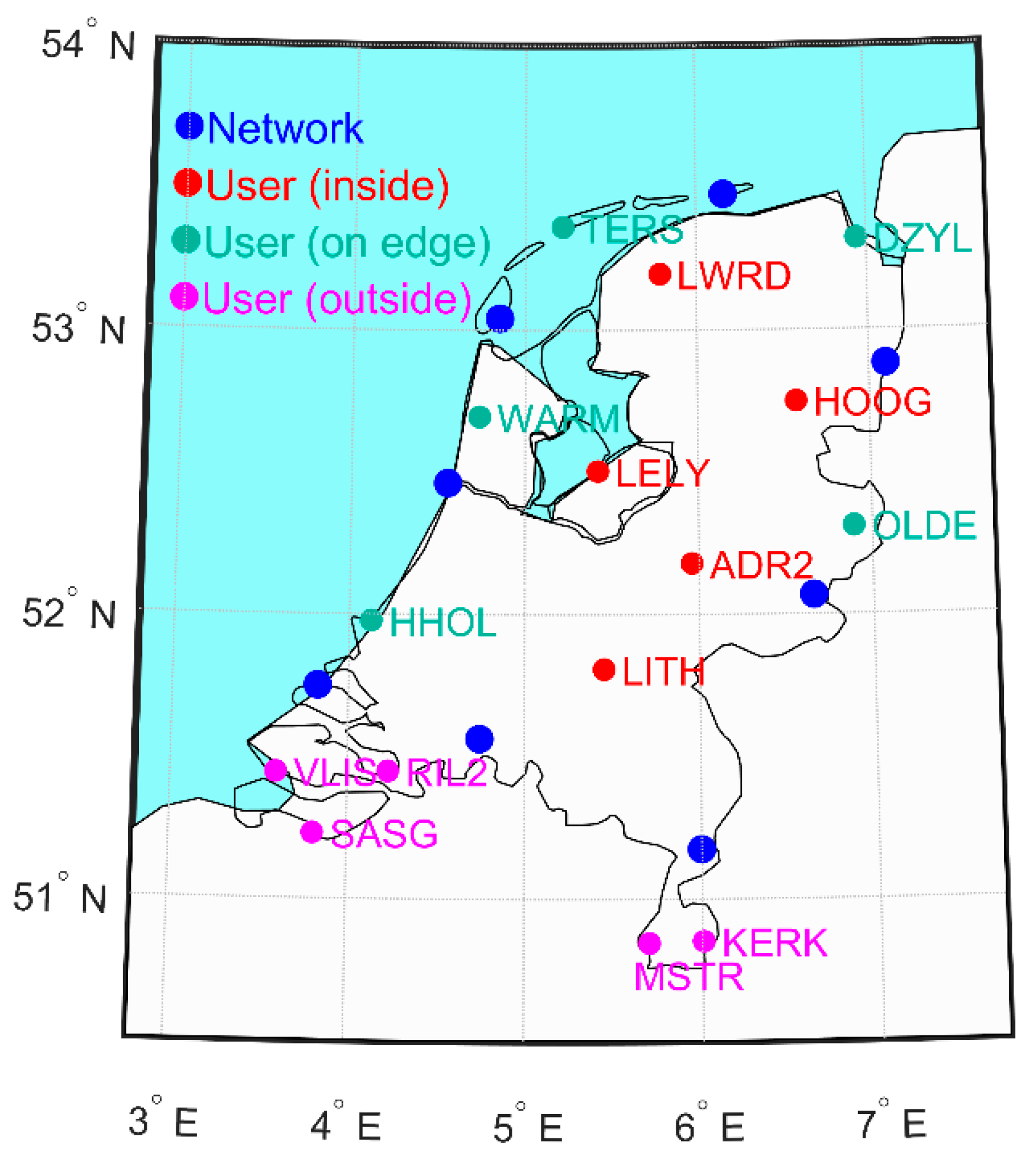
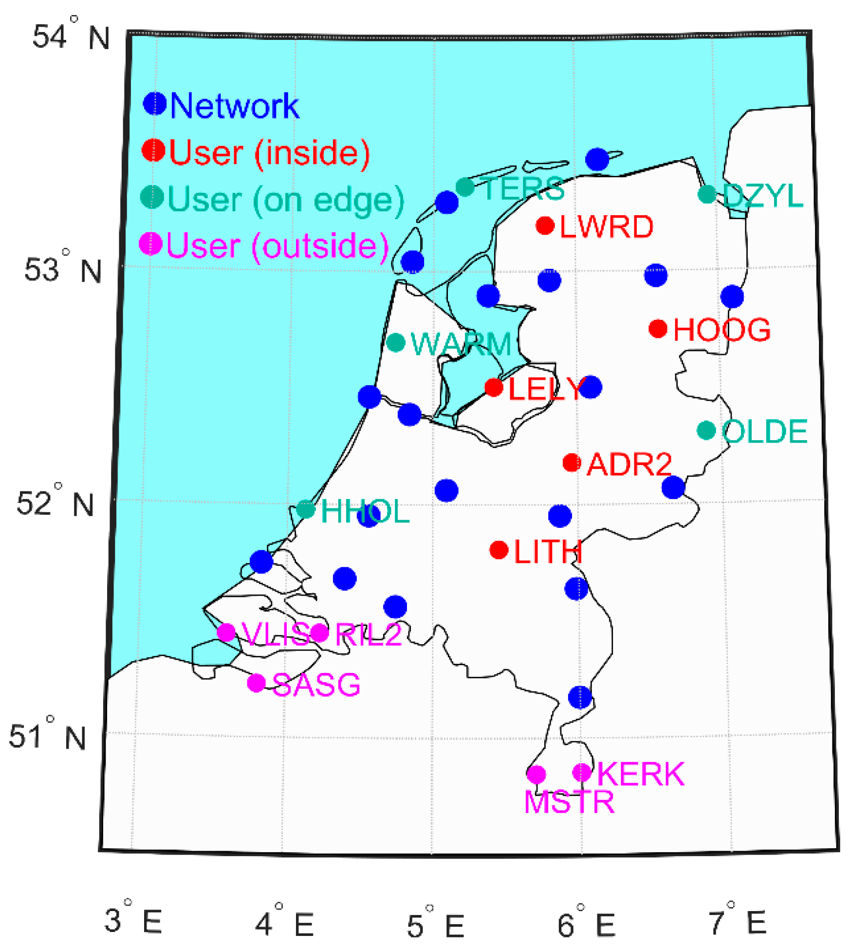
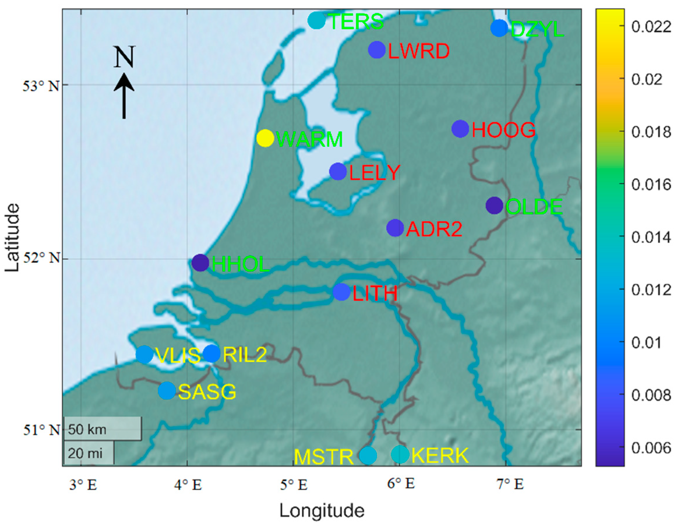
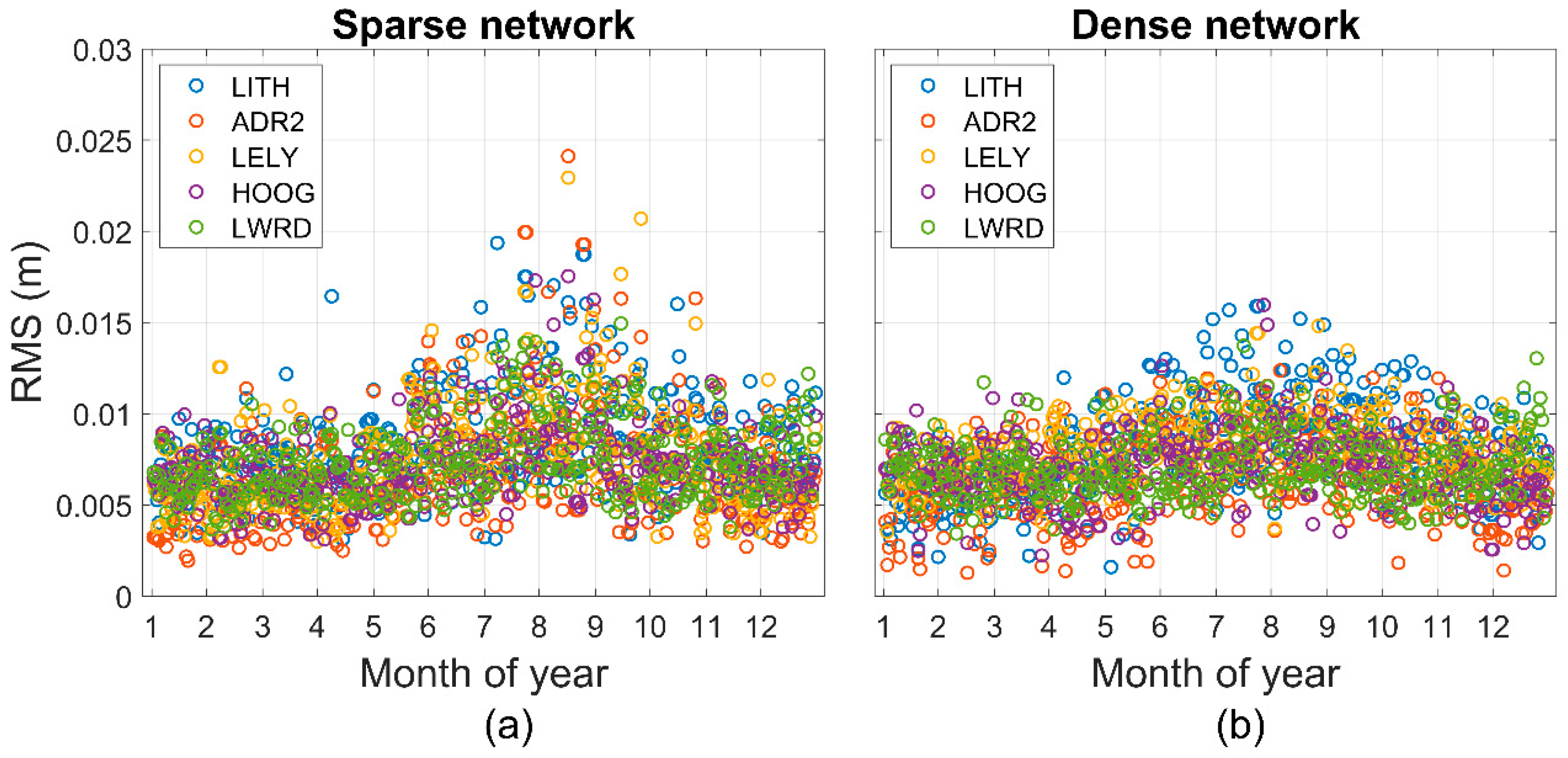
A sparse network with 8 reference stations and a dense network with 19 reference stations were selected in the CORS network of the Netherlands, as can be seen in Figure 1 and Figure 2, respectively. Distances between two nearby reference stations were varying, from $60 \mathrm{km}$ to $120 \mathrm{km}$ for the sparse network and $20 \mathrm{km}$ to $60 \mathrm{km}$ for the dense network. Another 15 user stations were also selected to evaluate the accuracy of the predicted zenith wet delays by comparing with the estimated delays at each user station. The total user stations are divided into three blocks: 5 stations (LWRD, HOOG, LELY, ADR2 and LITH) were inside the networks, 5 stations (TERS, DZYL, OLDE, HHOL and WARM) were on the edge of the networks and 5 stations (VLIS, RIL2, SASG, KERK and MSTR) were outside the networks. Therefore, the impacts of the locations can be investigated since the Kriging mainly depends on the distances between known and unknown points.

The IF combination-based Position and Navigation Data Analysis software (PANDA) [40,41,42] was used in this study to generate the zenith wet delay estimates at reference and user stations in the use of PPP data processing, and the configuration is shown in

Table 1. Summary of the strategy of data processing.

Parameter	Strategy and Value
Positioning mode	Static
Constellation	GPS
Frequency	L1 and L2
Satellite orbit and clock corrections	IGS
Interval	$60\mathrm{s}$
Kalman filter	Forward and backward
STD of phase/code observable	$0.005\mathrm{m}$/$0.5\mathrm{m}$
Weighting strategy	Elevation dependent
Zenith hydrostatic delay	Saastamoinen model
Zenith wet delay	Spectral density $0.02{\mathrm{m}}^2/\mathrm{h}$
Troposphere gradients	Spectral density $0.001{\mathrm{m}}^2/\mathrm{h}$
Ambiguity	Float

. Since the reference and user receivers were stationary, the static positioning mode was applied in this study with precise a priori coordinates so that the influence of the position errors would be attenuated. The dual-frequency GPS data were used in estimating the zenith wet delay. In addition, except for the coordinates, the dynamic models were also applied to the tropospheric wet delay and troposphere gradient parameters with the spectral density of $0.02{\mathrm{m}}^2/\mathrm{h}$ and $0.001 {\mathrm{m}}^2/\mathrm{h}$, respectively, based on their temporal properties.

This study applied precise satellite orbit and clock corrections provided from the international GNSS service (IGS) so that these two error sources were not considered in the positioning model. The interval of data processing was set to 60 s by taking into account the computational efficiency and the troposphere property that was temporally stable within a short time span. Since this was the post-processed PPP, forward and backward Kalman filter was applied; and thereby there was no convergence time at the beginning of data processing. Elevation-dependent weighing strategy was implemented due to the fact that signals at low elevation angles were likely to be affected by large model errors. The zenith hydrostatic delay has been corrected by the Saastamoinen model [8], and only the zenith wet delay was estimated. The ambiguities were always kept float in this study. One can refer to [43,44,45] for more information of fixing the ionosphere combined ambiguities.

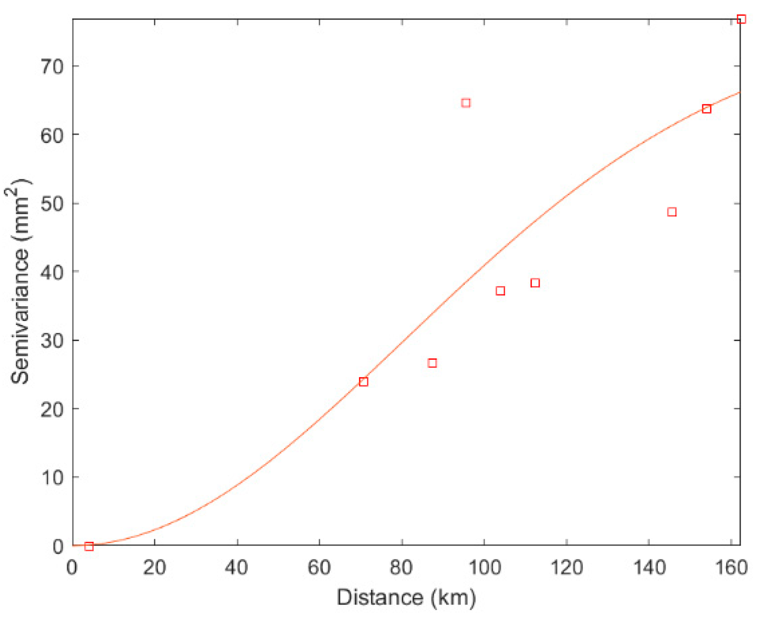
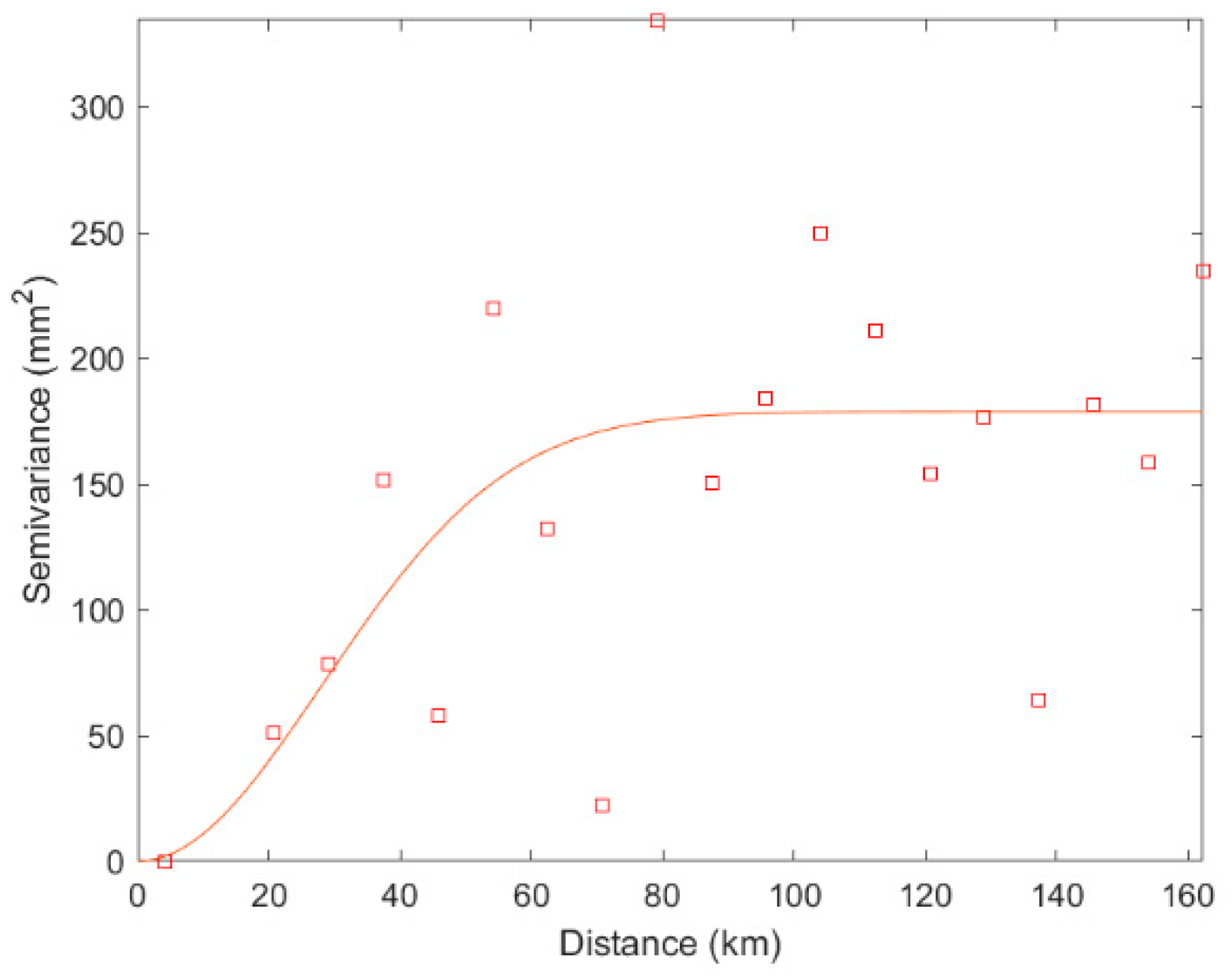
The data covering the entire year of 2019 were chosen to evaluate the performance of the Kriging interpolation, and the sample variogram of the sparse network and the dense network were estimated and presented in Figure 3 and Figure 4, respectively. Note that the fitted variogram models were determined at every epoch and used in Ordinary Kriging to predict the zenith wet delay at 15 user stations.

RMSEs of the 5 user stations inside the network between the predicted zenith wet delays and estimated delays are shown in Figure 5. The RMSEs of both the sparse network and the dense network during summer (July, August and September) period were larger than the rest of the months. This was reasonable since the water vapor content would change rapidly due to the rise of temperature, and, thus, the zenith wet delays may differ even in a small region. However, the dense network had a better performance in summer period than the sparse network by taking the advantage of the numerous stations. RMSEs exceed 1.5 cm with the sparse network were 1.75% of the sample, while with the dense network it is 0.33%. Overall, 84.38% of the RMSEs of the sparse network were less than 1 cm, and 88.49% of those for the dense network, which provide an adequate capability of predicting the zenith wet delay.

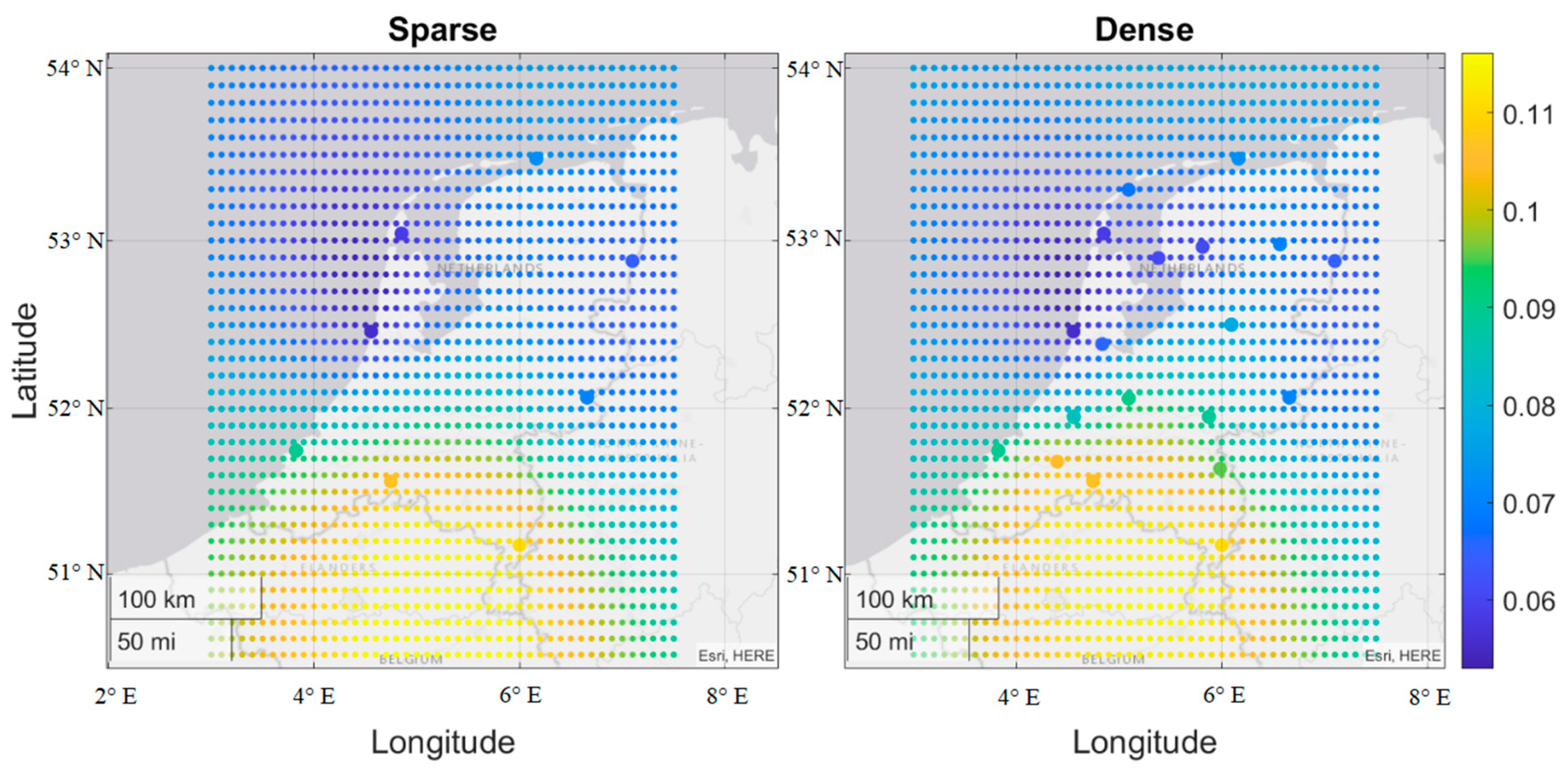
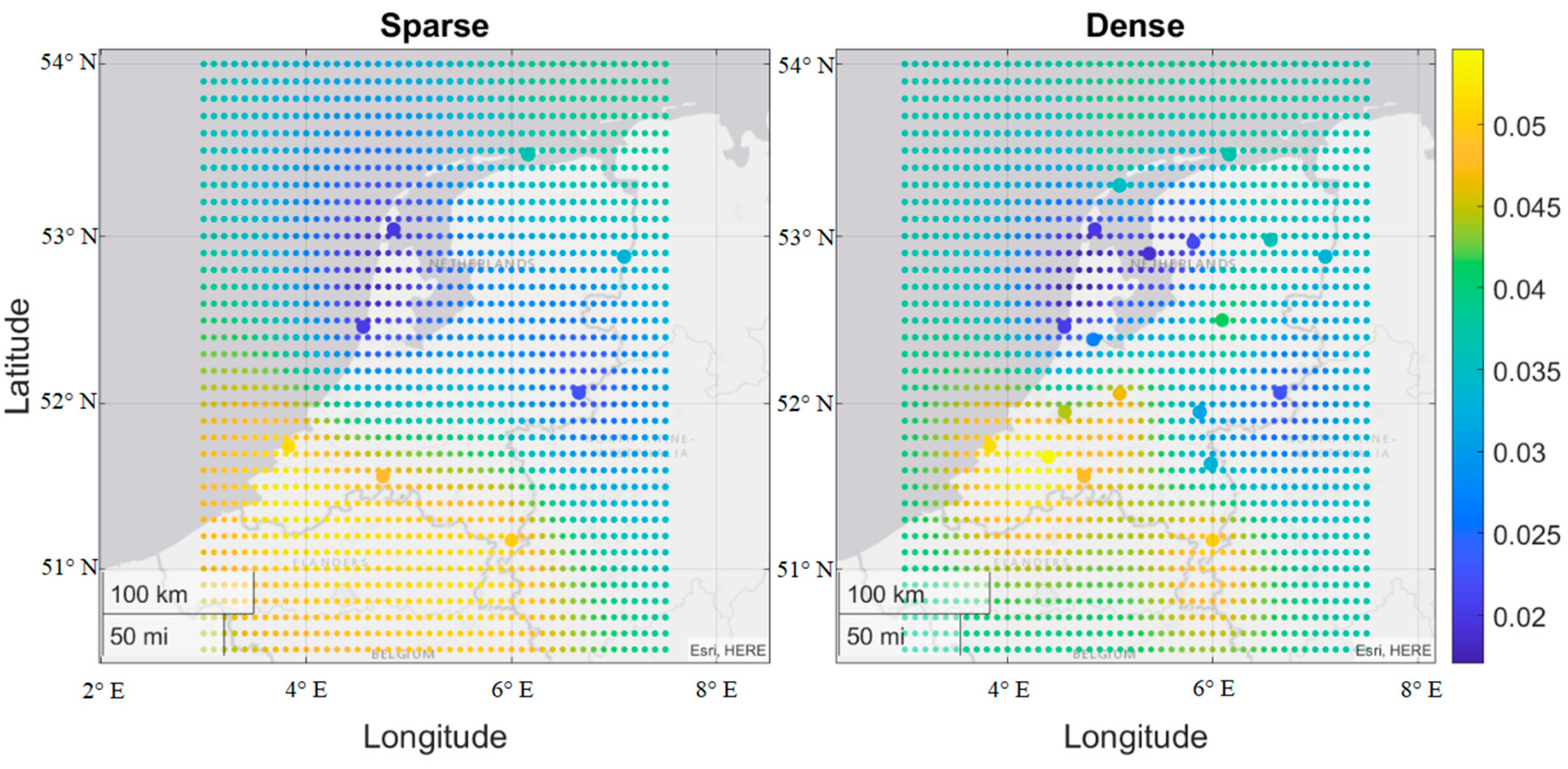
In order to justify the influences of the individual network on the predictions, the values of the predicted zenith wet delays at particular locations of the sparse and dense network during the winter period (1st February) and summer period (1st August) are presented in Figure 6 and Figure 7, respectively. Figure 6 presents that the pattern of the predicted zenith wet delays had a smooth surface so that a receiver at the same location of the sparse and dense network would have a similar predicted value. This indicated that the spatial variations of the water vapor were small and also explained the similar performances of the sparse and dense network under stable weather conditions.

On the contrary, the predicted zenith wet delays in the dense network were different from those at the same locations of the sparse network during the summer period, as shown in Figure 7. Since most of the newly added reference stations were inside the network, the elaborated description of the predicted zenith wet delays was presented as compared to the sparse network with fewer reference stations. Therefore, the predicted zenith wet delays are more accurate in the dense network than those of in the sparse network.

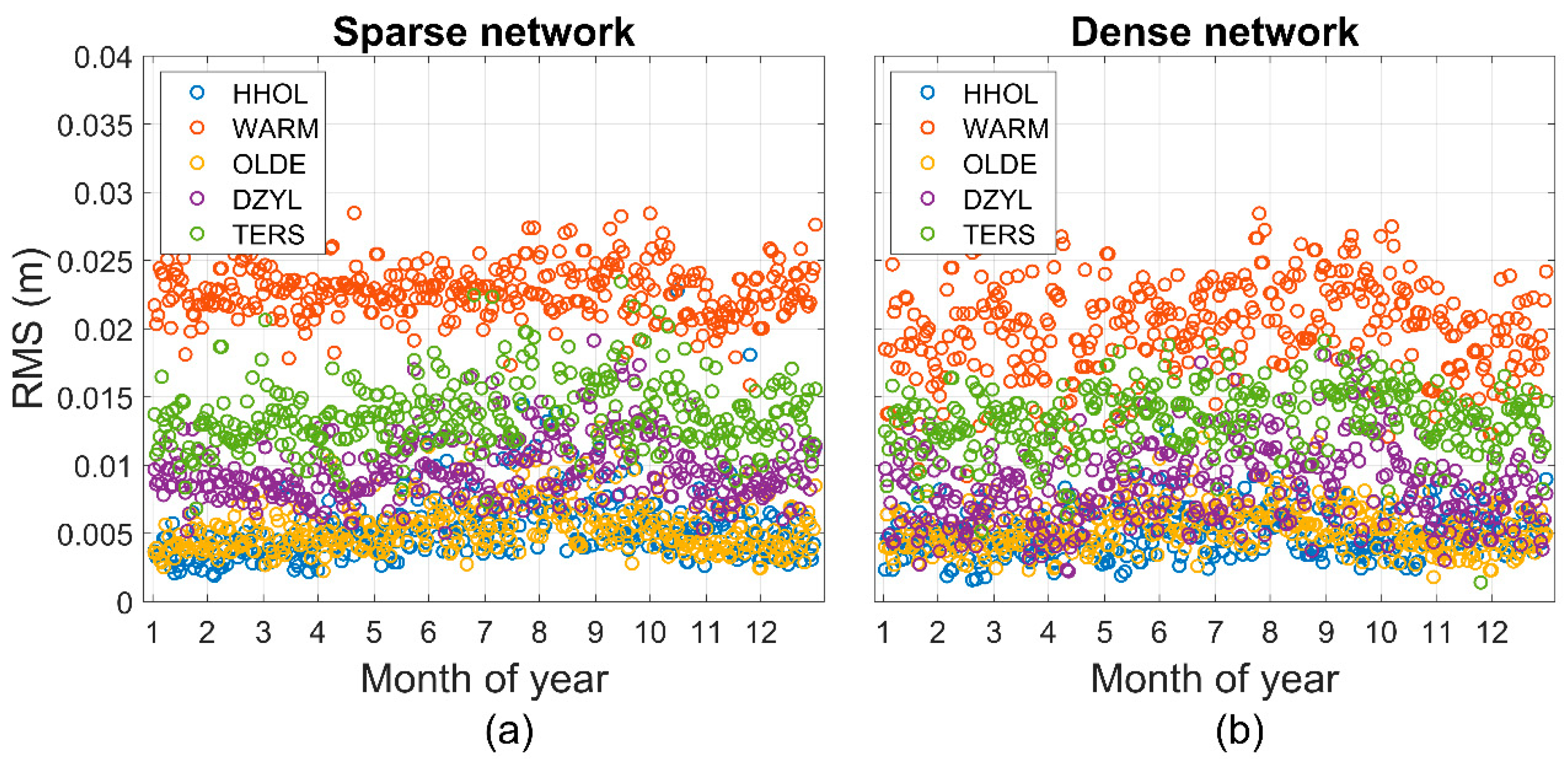
Figure 8 presents the RMSEs of the user stations on the edge of the network which were varying individually to each other. On the one hand, the zenith wet delay predictions of three stations HHOL, OLDE and DZYL were at the same accuracy level as the stations inside the network; and on the other hand, station WARM and TERS had significantly larger RMSE values than the others, as can be seen in Figure 9. This is because some of their nearby reference stations, shown in Figure 1 and Figure 2, were located in the coastal area or the islands, and, thus, the zenith wet delay estimations may change dramatically due to the water evaporation of the large water area. Besides, the seasonal variation was not significant for the stations WARM and TERS due to the inaccurate predictions.

Figure 9 indicates one exception of station HHOL which is located at the coastline while having small RMSE value. This was probably because the evaporation of the sea does not significantly affect the water vapor content above HHOL due to its location that one side was oriented towards the land. Comparatively, station TERS was on an island and WARM was on a “peninsula” between North Sea and Markermeer & IJmeer Lake. The large water area may disturb the smooth distribution of a local area, and, therefore, influenced the accuracy of the predicted zenith wet delays.

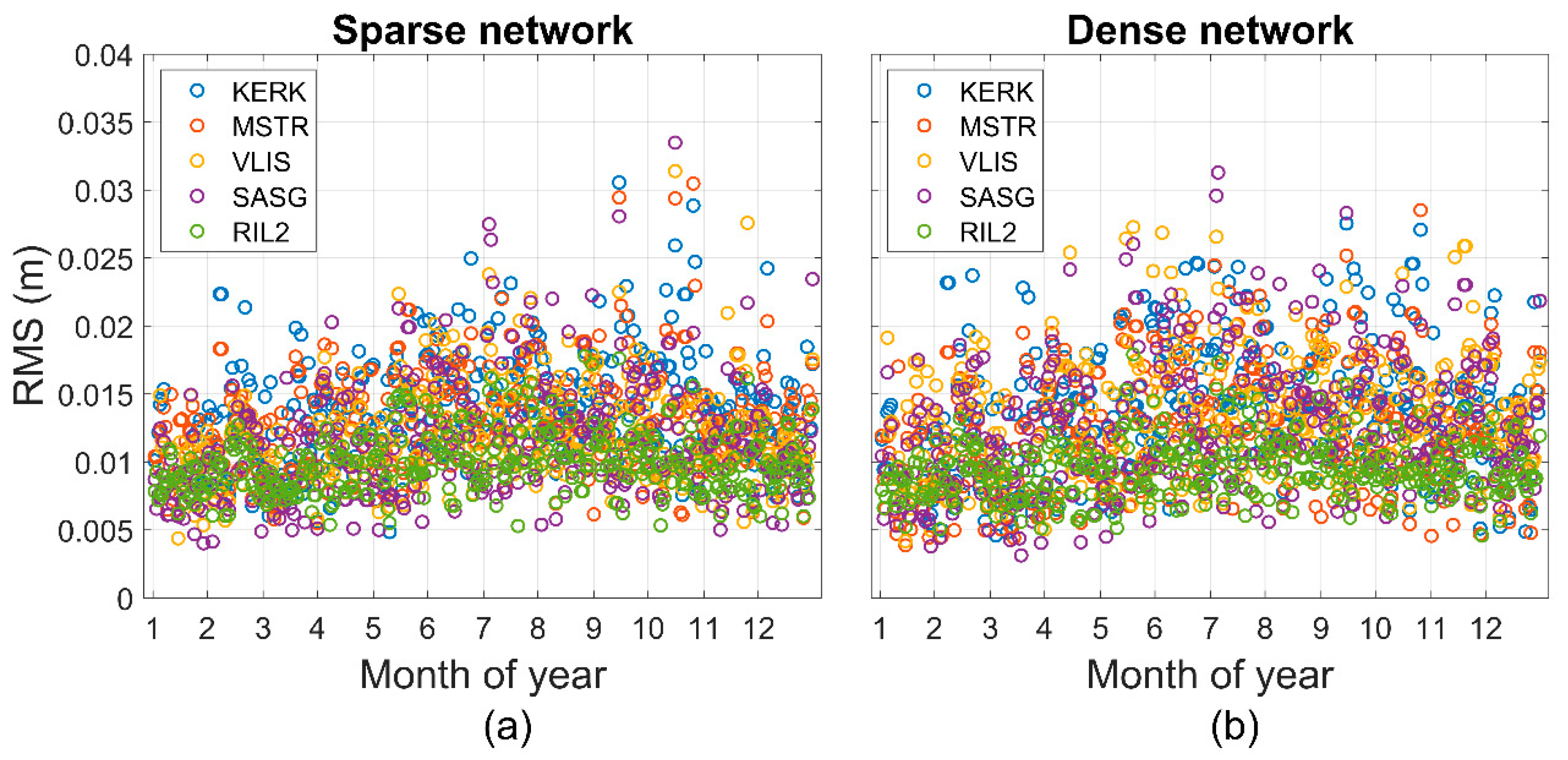
Figure 10 presents the RMSEs of the user stations that are outside the network. The patterns are likewise similar with an unobvious seasonal effect for both the sparse and dense network, which indicated that the number of reference stations had an insignificant impact on the stations outside the network. This was because the Kriging interpolation is a distance-based method, and the performances of the stations outside the network mainly depend on the closest reference station. 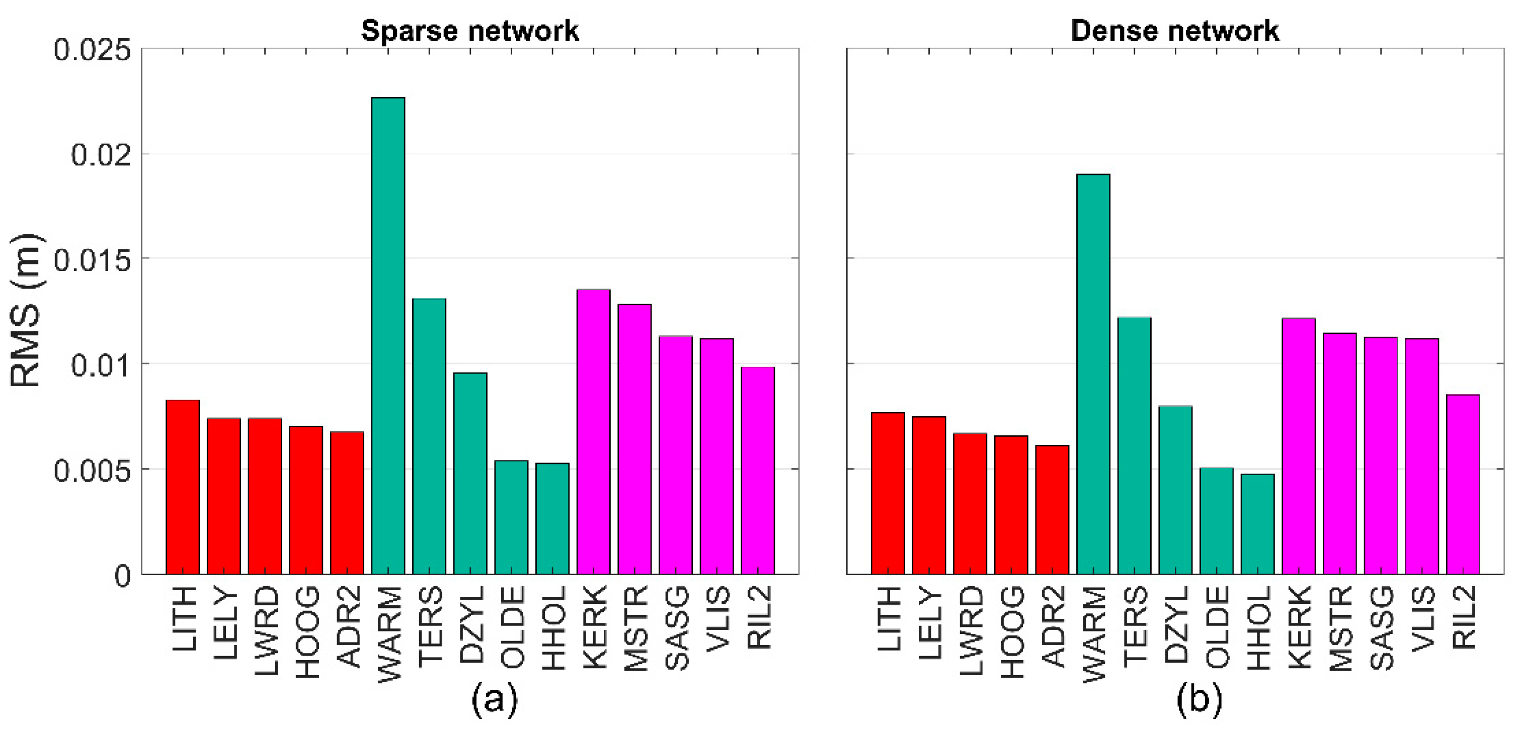For instance, as shown in Figure 11 the histogram of the average RMSE of user stations, KERK and MSTR have similar values because they have approximately the same distance to the reference station (as can be seen in Figure 1). Meanwhile, the other three stations VLIS, RIL2 and SASG were located closely with each other and, thus, have similar accuracies. RIL2 had the lowest RMS value among 5 stations outside the network because it had the shortest distance to the network station, and one newly added reference stations in the dense network were also close to RIL2, which improved the accuracy of this user station.

Table 2. Average RMSE of each user station. The unit is cm.

Region	User Station	RMSE of Sparse Network	Average	RMSE of Dense Network	Average
Inside	LITH	0.83	0.74	0.77	0.69
	LELY	0.74		0.75
	LWRD	0.74		0.67
	HOOG	0.70		0.66
	ADR2	0.67		0.61
On the edge	WARM	2.26	1.12	1.90	0.98
	TERS	1.31		1.22
	DZYL	0.96		0.80
	OLDE	0.54		0.51
	HHOL	0.53		0.48
Outside	KERK	1.35	1.17	1.21	1.09
	MSTR	1.28		1.14
	SASG	1.13		1.13
	VLIS	1.12		1.12
	RIL2	0.99		0.85

presents the statistics of the average RMSEs of all user stations. One can see that stations inside the network had sub-centimeter level accuracy, while stations on edge or outside the network attained the RMSEs around 1 cm. It is worth noting that the stations outside the network can also achieve 1 cm level accuracy, which was much better than the polynomial interpolation normally used in predicting the zenith wet delays. However, the benefits of the dense network were not evident because the water vapor content was spatially stable most of the time. The improvements offered by the dense network are 6.8%, 12.5% and 6.8% for the stations inside the network, on the edge of the network and outside the network, respectively.

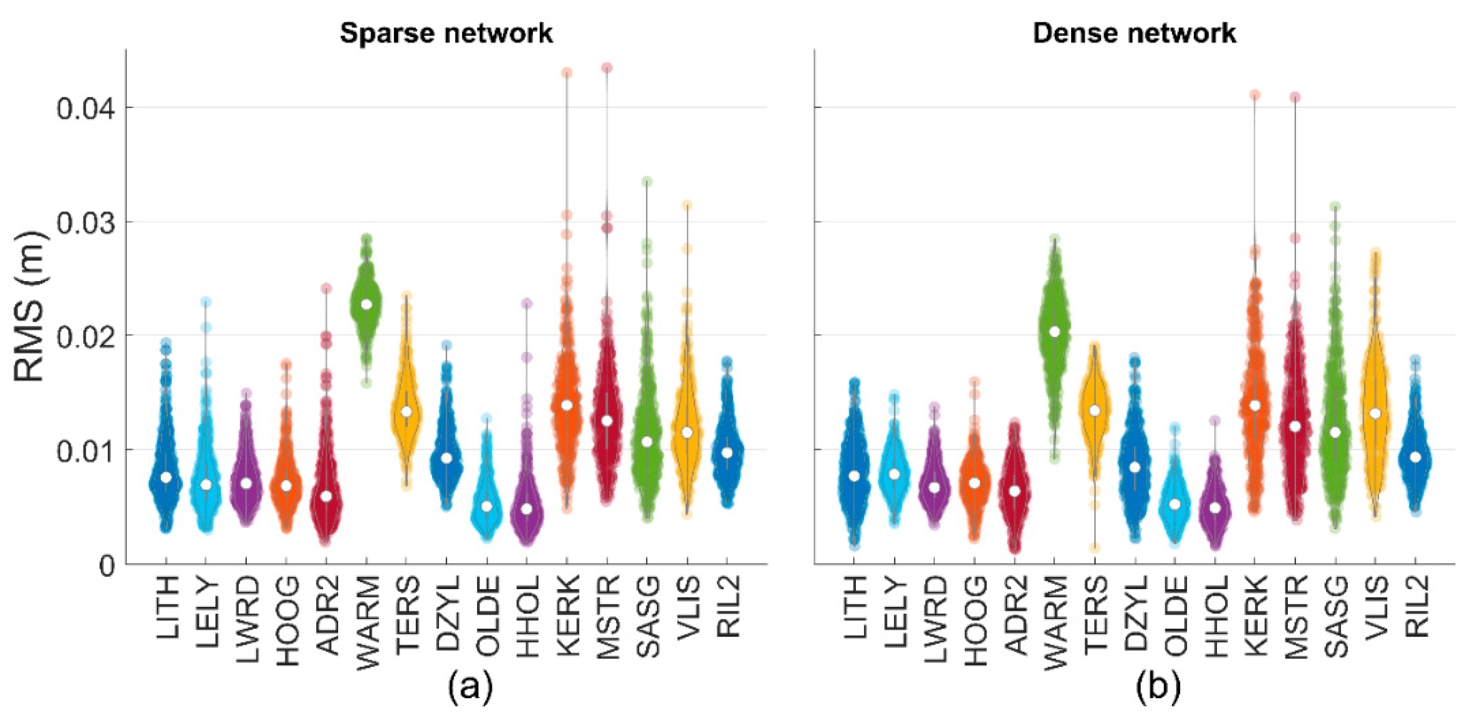
The violin plot [46] aims to summarize a batch of data by displaying several main features other than the average value. As shown in Figure 12 the violin plot of the RMSE values of all user stations in the sparse and dense network, it contains the fusiform of the density trace graphically showing the distributional characteristics of RMSEs for each user station and the circle showing the position of a typical central value. These two features summary the univariate data on spread and location.

As for the user stations inside the network, the lower adjacent values of three station LITH, HOOG and ADR2 in the dense network were smaller than those of the sparse network, indicating that the dense network can help provide more accurate predictions for the inland stations (i.e., the other two stations LELY and LWRD among 5 users stations inside the network were close to larger water area). Besides, most of the outliers in the dense network have disappeared because of the stable predictions during summer period.

The RMSEs distribution of station WARM in the dense network saw a significant improvement, in that, the first quartile was much lower than that of the sparse network, even though their central values were almost at the same accuracy level. Other two stations on the edge of the network TERS and DZYL had better performances in the case of the dense network in terms of the lower adjacent value and the first quartile. However, the patterns of the stations outside the network did not change much between the dense or sparse network, indicating a low sensitivity of the stations outside the network to the number of the references.

4. Conclusions and Discussions

This contribution investigates the performances of the Kriging interpolation in predicting the zenith tropospheric wet delays in the use of GNSS networks. The zenith wet delay was estimated in PPP data processing with the IF combination model at the selected Netherlands CORS stations. A sparse network with 8 reference stations and a dense network with 19 reference stations were selected and used to predict the zenith wet delays at 15 user stations, including 5 inside the network, 5 on the edge of the network and 5 outside the network.

The entire year’s data of 2019 were processed to evaluate the quality of the zenith wet delay predictions from the Kriging interpolation, and the RMSEs were calculated by comparing the predicted delays and the estimated delays at each user station. The RMSEs of 5 user stations inside the network were at sub-centimeter level, in which average values were 0.74 cm with the sparse network and 0.69 cm with the dense network. The stations on the edge of the network achieve 1 cm accuracy level with 1.12 cm of the sparse network and 0.98 cm of the dense network. The statistics of RMSE were 1.17 cm with the sparse and 1.09 cm with the dense when user stations were outside the network.

The seasonal effects can be seen in the user stations inside the network that the accuracy of predicted zenith wet delays is relatively worse in summer period because water vapor content would change rapidly in space with the rising temperature. Results also show that the benefits of the dense network are not evident for the average RMSE over the year as the water vapor content is spatially stable most of the time. Compared to the sparse network, the number of dense network stations is doubled; meanwhile, the average RMSE is reduced by around 10%. The advantages of the dense network are mainly in the summer period and the stations that are encountered complex weather conditions.

As for the user stations inside or on the edge of the network, the performances of the inland stations are usually better than those of coastal because of the inland smooth water vapor disturbances. The prediction accuracy of the stations outside the network mainly depends on the distance to the nearby reference station, therefore it is not sensitive to the number of reference stations.

The predicted zenith wet delays can be used in strengthening the PPP models to improve the positioning accuracy and reduce the convergence time and used in NWP models to help identify model biases and forecast weather conditions. Although the Kriging interpolation has been confirmed for a certain level of accuracy for predicting the zenith wet delays using a GNSS network, the conclusions of this contribution are restricted by the number of CORS stations and the area of the Netherlands. More stations or a larger area might be needed in further investigation of the Kriging interpolation in predicting the zenith wet delays or other GNSS applications.