1. Introduction
A north–east cold vortex (hereafter referred to as a cold vortex) is a closed, upper-tropospheric, low-pressure system that is completely detached from its polar source and extends to the south of the mid-latitude westerly mean flow as a result of the deepening of a high-level trough [
1]. It is formed following a rapid intrusion of cold air into the upper west-wind belt from the north and strengthened by a cyclonic rotation of the wind upstream and a strong wind around the cold dome in the south [
2]. A cold vortex is an important weather system that causes low temperatures and sometimes also large amounts of rain [
3,
4,
5]. It also plays an important role in the stratosphere–troposphere exchange of trace gases, such as ozone and hydrocarbons [
6,
7]. Therefore, cold vortices have been studied for different reasons.
The climatological features of warm season cold vortices in East Asia include their distribution, size, origin, temporal variations and their influence on rainfall and severe weather [
5,
6,
7,
8]. The detailed analysis of the evolution of the north vortex and the interactions between the north vortex and other systems indicates that different factors dominate in various stages of its evolution, such as eddy flux circulation and the eddy kinetic energy budget [
9]. The formation of north–east cold vortex circulation was found to be closely associated with various types of ridges or blocking-type circulations [
10]. Simulations with the Advanced Research Weather Research and Forecasting (ARW) numerical model show that latent heat is very important for the development of a cold vortex and intensity changes [
11]. The vertical advection of vorticity, which is closely related to convective activity, is the most favorable factor for maintaining a cold vortex [
12].
A study of the horizontal and vertical structures of an upper air cold vortex showed that the center of the vortex is cooler than the periphery in the middle troposphere and the relative vorticity is greatest just below the tropopause [
13]. The distribution of precipitation has been addressed in several studies, leading to different conclusions. Sun et al. [
10] concluded that precipitation tends to concentrate in the southeastern quadrant of the circulation, whereas other studies show that heavy rainfall mainly occurs to the east of the circulation center [
14] or in the northeast of the vortex center [
15]. By comparing three cases of cold vortex circulations and their rainfall patterns, Zhao and Sun showed that the rainfall pattern varies with the type of vortex [
16].
Many studies have been conducted on the macro-physical properties of cloud systems triggered by cold vortices, but much less attention has been paid to microphysical processes. Microphysical processes are important during the formation and development of a cloud system. The interactions between hydrometeors affect the entire dynamical and thermo-dynamical cloud system [
13,
17] because latent heat absorbed or emitted in cloud microphysical processes modifies buoyancy, which in turn contributes to the development and maintenance of vertical air motion [
18,
19,
20,
21]. Ice microphysics—and, in particular, the melting effect—can play an especially important role in the generation of the mesoscale structure and evolution of weather systems and rainfall [
18,
20,
22]. Ice microphysics processes and ice phase precipitation are discussed in detail by Gultepe et al. [
23,
24]. The distribution characteristics of microphysical elements, the growth mechanism of precipitating particles and the evaporation effects of sub-cloud raindrops in cold vortex processes have been addressed in studies by Chen et al. [
25], Zhou et al. [
26] and Zhao and Lei [
27]. However, the microphysical processes in a cold vortex are still quite unclear.
In this paper, we address the microphysical processes in a strong cold vortex. The cold vortex system was simulated using the Weather Research and Forecasting (WRF) model described below. It formed at high latitude (58° N, 96° E), moved towards the east and separated into two parts—a northern and a southeastern cloud band—before it dissipated. The lifetime of the vortex was four days, from 20 May to 24 May 2018, and it produced a large amount of precipitation along its trajectory, influencing several thousands of kilometers. The distribution of the precipitation and microphysical features were investigated during the entire lifespan of the cold vortex while it moved to the east. After introducing the model in
Section 2, the synoptic conditions and the structure and precipitation characteristics of the cloud system are described in
Section 3. The microphysical properties are presented in
Section 4, with different sections for the southeastern cloud band (
Section 4.1) and the northern cloud band (
Section 4.2). Conclusions from the study are presented in
Section 5.
2. Model
2.1. Model Details
The Weather Research and Forecasting (WRF) model V4.0 [
28] is a fully compressible, non-hydrostatic atmospheric model that is widely used in operational forecasting and atmospheric research. It is designed for a broad range of applications across scales ranging from meters to thousands of kilometers, and so it can be used for the simulation of both mesoscale systems and microphysical processes. The microphysical schemes in the WRF model include some relatively complex processes that are suitable for examining detailed cloud microphysics.
The cold vortex system studied in this paper covered a large area of several thousands of kilometers during its movement from west to east within four days from 20 May to 24 May 2018. Considering the large-scale cloud system and high temporal–spatial resolution needed to study the cloud physical features and rainfall processes, two-way interactive domains were used (as shown in
Figure 1). The first domain, d01, centered on (50° N, 115° E), with 350 × 250 grid points and a horizontal grid resolution of 18.0 km, was used for macrophysical properties. The second domain, d02, centered on (50° N, 120° E), with 733 × 550 grid points and a horizontal grid resolution of 6.0 km, was used to study microphysical properties.
The cloud microphysics scheme chosen in the simulation was the “NSSL 2-mom+CCN” scheme [
29]. The “NSSL 2-mom+CCN” scheme is one of the most detailed microphysics schemes compared to other schemes in the WRF model, and it is effective for use in microphysical studies. This scheme considers different microphysics processes such as cloud droplet initiation and growth, autoconversion, accretion, rain freezing, ice crystal initiation, terminal fall speed, graupel bulk density, ice initiation of graupel, two-component collection, self-collection, ice conversion to snow, graupel conversion to hail and reflectivity conservation. Each process includes a large number of parameters which are different for each process, as described in detail by Mansell et al. [
29]. The scheme can predict two independent moments (mass and number concentration) for six hydrometeor types (cloud droplets, rain, ice crystals, snow, graupel and hail). It also predicts the bulk concentration of cloud condensation nuclei (CCN) as well as the average bulk densities of graupel and hail.
The cumulus parameterization scheme used in the first domain was the Kain–Fritsh scheme [
30], and no cumulus parameterization was used in the second domain. The high-resolution YSU scheme [
31] was used to describe the planetary boundary layer physics in the model. The YSU PBL increases boundary layer mixing in the thermally induced free convection regime and decreases it in the mechanically induced forced convection regime; thus, some systematic biases of the large-scale features could be resolved. The New Goddard scheme [
32] was adopted to describe radiation processes. A time-dependent boundary condition was used in integral calculation.
The initial and boundary conditions for the simulation were established by interpolating the National Centers for Environmental Prediction (NCEP) 1° × 1° 6 h interval reanalysis data onto the study domain. The simulation was run for 96 h starting from 0000 UTC on 20 May 2018, and the outputs for the first (and second) domain were exported every 30 (10) min.
2.2. Macro Comparison of Observations with Simulations
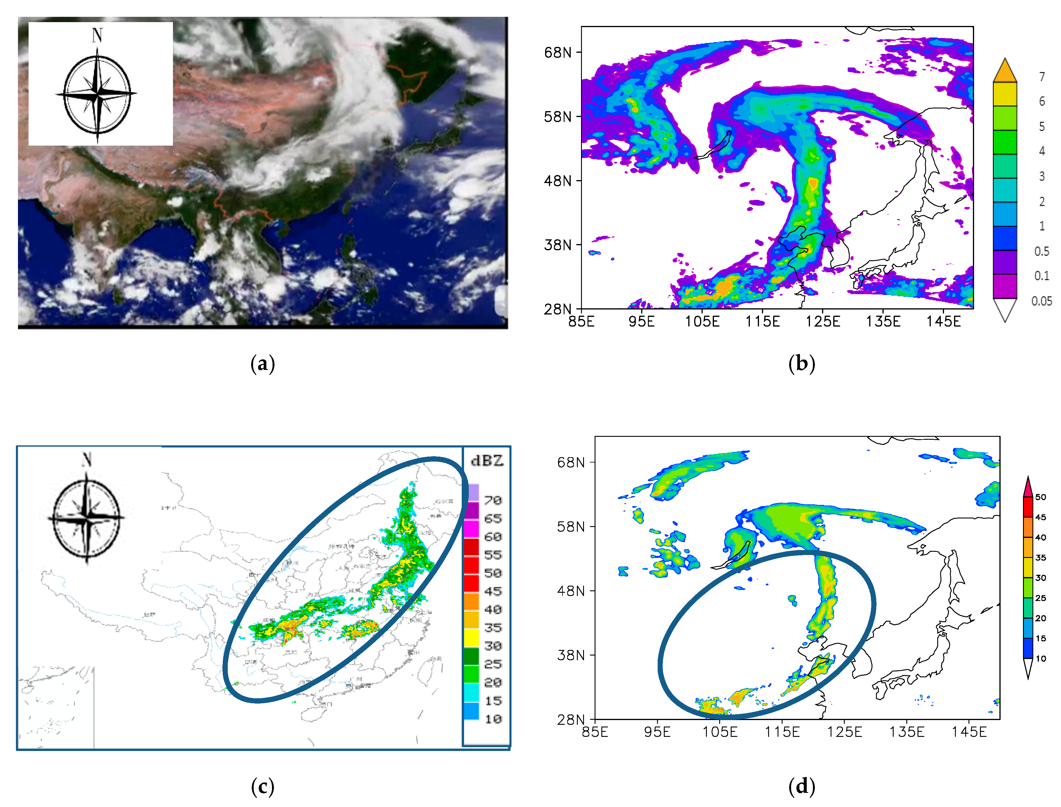
The cold vortex developed on 20 May 2018. The associated cloud belts developed and moved from west to east, bringing large-scale inhomogeneous rainfall over the affected region. This is illustrated in
Figure 2, which shows both satellite and radar observations, as well as model simulations of the observed features.
Figure 2b shows the simulated total liquid and solid water content (g/kg) integrated over all layers and derived from the first-domain simulation at the time when the storm developed most vigorously: on 22 May at 02:00 UTC, 50 h after the start of the simulation. The satellite image observed at this time by the FY-II satellite is shown in
Figure 2a. The rectangles in
Figure 2a,b encompass approximately the same area, and the features of the simulated cloud system inside the rectangle are similar to those observed by the satellite.
The first-domain model calculations were also used to simulate the radar echo in dbz [
33], as presented in
Figure 2d, which was compared with the Plan Position Indicator (PPI) mosaic product of radar reflectivity (
Figure 2c) obtained from the Chinese meteorological information center. This PPI product only shows the distribution of the radar reflection from the cold vortex cloud and precipitation system along the track over China, but not outside of China.
Figure 2c shows the curvature of the cloud belt and its uneven distribution. Most radar reflectivity was in the range of 20–25 dbz, and the highest embedded reflectivity was 45 dbz. The simulated reflectivity (in the elliptical domain in
Figure 2d) agrees with the observations at that time.
The good agreement of the simulated and observed macrophysical features illustrates the suitability of the model to study this cold vortex system.
3. Case Review
3.1. Synoptic Condition
The synoptic situations during the formation of the cold vortex on 20 May 2018 and at the end of the study period on 24 May 2018 are presented in
Figure 3.
Figure 3 shows the 500 hPa geopotential heights (contours, gpm) and wind vector fields provided at 6 h intervals from the National Centers for Environmental Prediction (NCEP) global reanalysis product at a 1° × 1° resolution.
During formation, the center of the cold vortex was located at 56° N, 93° E (
Figure 3a) and moved from west to east. During the movement, the vortex split into two centers, which on 24 May were located at 63° N, 106° E and at 48° N, 136° E (
Figure 3c). Accompanying the vortex, a cold front and a warm front developed at the surface. The vortex, together with the cold and warm fronts, triggered a large-scale cloud system and extensive precipitation process.
3.2. Structure and Precipitation Characteristics of the Cloud System
The cloud system associated with the cold vortex system formed, strengthened, split into two and dissipated during the movement from west to east and led to extensive rainfall in the affected region. This is illustrated in
Figure 4, which shows the 500 hPa wind vectors, together with the horizontal distributions of the simulated clouds at the same pressure level, at 2, 24, 48, and 67 h after the start of the simulation (
Figure 4a–d). The position of the cold vortex and the associated clouds are indicated by the black rectangles in
Figure 4a–d.
Figure 4a shows that the cloud system formed around the vortex, with its center at 58° N, 96° E 2 h after the start of the simulation, with broken cloud bands to the southeast and a continuous and even cloud band to the north of the vortex. The clouds were not heavy during the formation of the system, with a radar reflectivity of 5–15 dbz from most parts of the clouds and a maximum radar reflectivity of 25 dbz locally. The simulation shows that light rain started right after the formation of the cloud system.
The cloud system moved with the vortex towards the east, and 24 h after the start, its center was located at approximately 55° N, 105° E. The cloud system developed into a larger system, and the maximum radar reflectivity of 25 dbz covered more areas than during the formation period, as shown in
Figure 4b. Additionally, the southeast cloud area was larger than the northern band.
When the vortex system traveled further to the east, the rotation of the vortex axis caused a further extension of the cloud system in the south–north direction and covered a larger area, as shown in
Figure 4c.
Figure 4c shows the situation after 48 h, when the cloud system covered more than 3500 km along the south–north direction and 3000 km along the east–west direction, with the vortex center at 55° N, 115° E and a maximum radar reflectivity of 35 dbz in the southern part.
The vortex cloud system rotated further, split into two parts and dissipated during the movement.
Figure 4d shows the situation after 67 h, when the vortex center was located at 53° N, 120° E. One cloud band was situated along the southeast of the vortex, and the other cloud band was situated along the northwest of the vortex; the maximum radar reflectivity of both cloud bands was 25 dbz.
The whole cloud system lasted for four days and brought precipitation over a large area, and the precipitation was not evenly distributed.
Figure 4e,f show the spatial distributions of the amounts of liquid and solid precipitation integrated over all four days. North of 48° N, mixed liquid and solid precipitation was exhibited, with a maximum amount of both liquid and solid precipitation of more than 40 mm; south of 48° N, mainly liquid precipitation was present, with a very small amount of solid precipitation, and the maximum amount of liquid precipitation was more than 40 mm. The liquid precipitation covered the whole area affected by the cloud system, while the solid precipitation covered a much smaller area—mainly at high latitudes—influenced by the northern cloud band. Only a small amount of solid precipitation was produced by the southeastern cloud band.
4. Microphysical Properties of the Vortex Cloud System
As discussed above, the cloud system distribution was not evenly distributed. The northern cloud band was mainly influenced by a warm front and produced mixed liquid and solid precipitation, and the southeastern cloud band was mainly influenced by a cold front and produced liquid precipitation, with limited solid precipitation north of 48° N. Additionally, the southeastern cloud part developed more vigorously than the northern cloud part for most of the time and produced heavier precipitation. Therefore, microphysical processes are discussed for each cloud system separately.
To reveal the interior structure of the clouds and their microphysical features, vertical cross-sections were taken zonally, as shown in
Figure 5,
Figure 6,
Figure 7,
Figure 8,
Figure 9,
Figure 10 and
Figure 11. In this paper, six hydrometeor types (cloud droplets, rain, ice crystals, snow, graupel and hail) were simulated, and the hail mixing ratio was 0 g/kg during the whole process; thus, the vertical distribution of hail is included in these pictures.
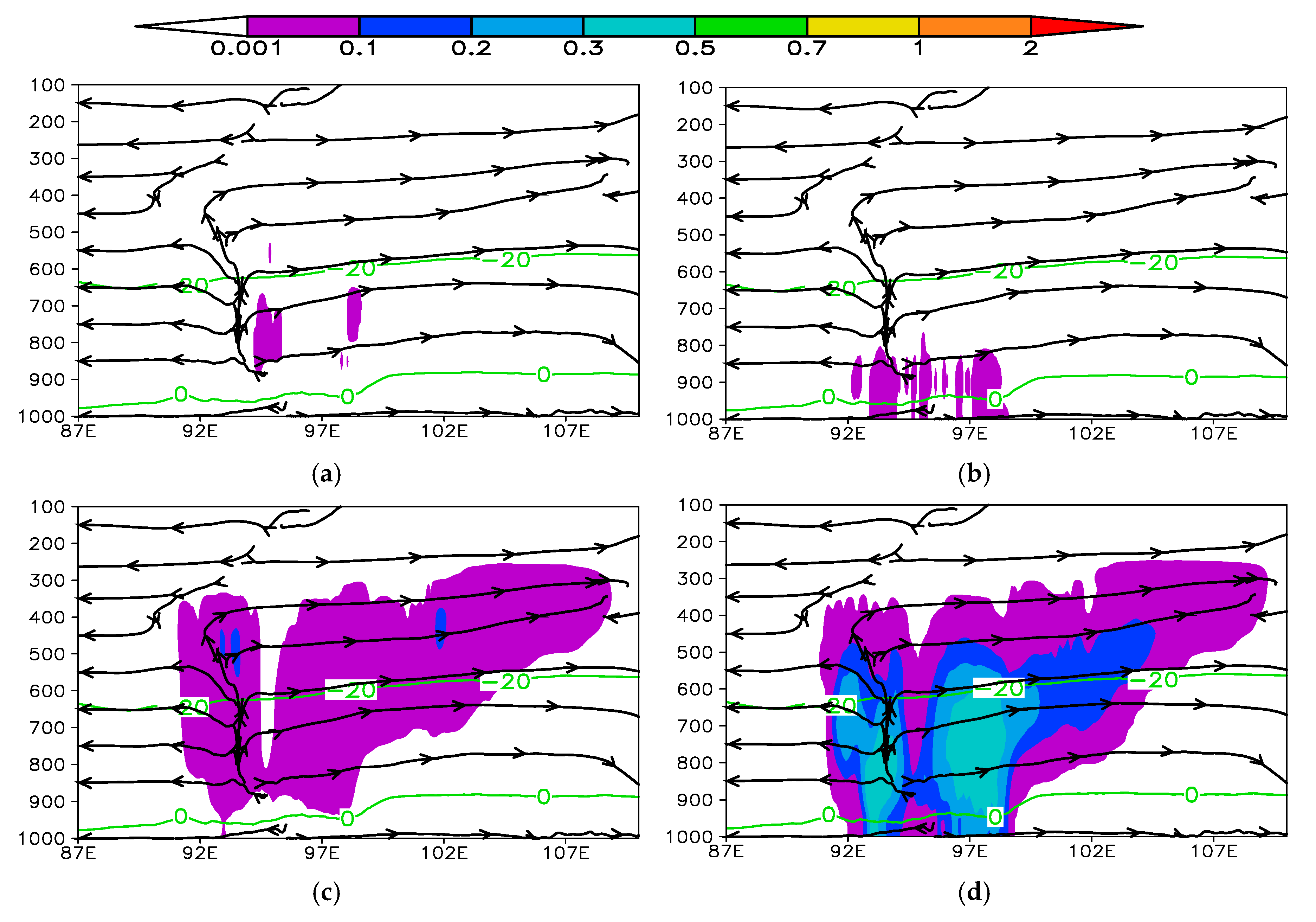
4.1. Microphysical Properties of the Southeastern Cloud Band
4.1.1. The Formation Period
As shown in
Figure 5a–e, the water content (liquid or solid) along the black line in
Figure 4a was low during the formation period (at the model time of 2 h), with several areas with a high water content. The system produced only light liquid and solid precipitation that reached the surface. The southeast cloud area developed to high altitudes even in the formation period—sufficiently deep to reach 250 hPa.
Among the hydrometeors, the mixing ratio of the liquid phase—i.e., cloud and rain droplets—was very different from that of the solid phase (ice, snow and graupel), as shown in
Figure 5a–e. This cloud system was very cold, and the 0 °C; level was very low, leading to cold cloud physics dominating the whole system. The cloud water mixing ratio covered only a small area, with a maximum of 0.2 g/kg in some cloud regions. The rain mixing ratio was very small, at 0.001 g/kg, and existed mainly in small areas below 800 hPa. There were almost no rain droplets at higher levels because there were insufficient cloud droplets available for coalescence, and the rain droplets below the clouds probably resulted mainly from the melting of solid particles.
Most of the cloud area was covered by ice and snow particles, as shown in
Figure 5c–e, with areas in which the maximum ice and snow mixing ratios were 0.1 and 0.5 g/kg, respectively. The cloud band was in a low-temperature environment, so there were abundant solid particles. After the solid particles formed, they could grow to larger sizes through cold cloud microphysics processes such as deposition, accretion, aggregation [
23,
24] or the Bergeron process [
34]. Because there was only a small amount of cloud droplets available, the solid particles did not grow sufficiently large to form graupel through accretion (
Figure 5e). Graupel was only formed in small amounts below the cloud system, and the maximum mixing ratio was 0.001 g/kg, which means that graupel only formed below clouds through accretion when the solid particles fell through the clouds.
The data in
Figure 5 and the discussion above show that, during the formation of the cold vortex, cold cloud processes dominated the precipitation period and that precipitation was a mixture consisting mainly of rain formed by the melting of solid particles, along with some particles which remained in the solid phase. The precipitation from the southeast cloud band during the formation period consisted mainly of mixed liquid and solid precipitation.
4.1.2. The Development Period
The vertical distributions of the mixing ratios for the different components contributing to the total liquid and solid water content during the development period, at the model time of 24 h, were evaluated along the black line in
Figure 4b. The results are presented in
Figure 6a–e. The data in
Figure 6 suggest that the cloud system developed quickly and extended over a large area, with a peak total water content greater than 2 g/kg. The cloud system developed deep into 200 hPa, located north of 48° N (east of 106° E in
Figure 6) and produced a large quantity of mixed solid and liquid precipitation. The cloud band south of 48° N produced mainly liquid precipitation.
Even though there were abundant hydrometeors, the liquid water content covered only a small area in contrast to the solid water content, which dominated the cloud system, as shown in
Figure 6a–e. The cloud droplet mixing ratio covered many smaller areas inside the cloud band, with a maximum mixing ratio of 0.2 g/kg, indicating that few cloud droplets were formed and that they were efficiently consumed by coalescence, the Bergeron process or accretion. There were very few rain droplets inside the clouds. Below the clouds, rain droplets occurred with a maximum mixing ratio of 0.3 g/kg over the area around 115° E. This means that rain droplets were hardly formed by coalescence, because there were insufficient cloud droplets, and the rain droplets below the cloud were mainly formed by the melting of solid particles.
Ice and snow were present throughout the whole cloud system, with maximum mixing ratios of 0.1 and 2 g/kg, respectively, meaning that cold cloud processes dominated the microphysical processes. Even though the solid particles covered most of the cloud area, there were fewer below the clouds; ice particles did not reach the ground at all, and snow particles covered a large amount of the area under the clouds, with some reaching the ground. This distribution of solid particles meant that a large number of them melted into liquid droplets, and some of the snow particles still remained in the solid phase until they reached the ground. The graupel only formed in a small area inside and below the clouds, with a mixing ratio peaking at 0.001 g/kg, which means that accretion did not contribute sufficiently to produce larger particles because there were insufficient liquid particles to support this process.
Overall, the distribution of hydrometeors during the development stage implies that precipitation consisted mainly of rain formed by the melting of solid particles, along with some snow particles and graupel. During the first day of the simulation, the southeastern part mainly produced liquid and solid precipitation.
4.1.3. The Maintenance Period
During the maintenance period, the cloud system rotated and started to develop into a dual system with one cloud band in the north, elongated in the west–east direction, and another one to the southeast extending in the north–south direction, as shown in
Figure 4c. The vertical cross-sections of all hydrometeor mixing ratios in the southeastern cloud system in
Figure 7 show that the hydrometeor center was not as strong as in the development period, with a maximum mixing ratio of less than 1 g/kg. The cloud system still extended as deep as 200 hPa.
The cloud droplets were mainly distributed to the south of 45° N, where the temperature was higher, with a maximum mixing ratio of 0.5 g/kg, as shown in
Figure 7a. The rain droplets were distributed over several areas. The area located to the south of 37° N included both rain droplets and cloud droplets, with a maximum cloud droplet mixing ratio of 0.3 g/kg, as shown in
Figure 7b. The co-occurrence of rain droplets below the cloud and cloud droplets in the cloud meant that the cloud droplets grew into rain droplets through coalescence and produced liquid precipitation. The other rain droplet center between 42° N and 46° N was below part of a snow center, which meant that snow particles melted to produce rain droplets. The distribution of cloud and rain droplets shows that there were more liquid droplets during the maintenance period than during the development period; consequently, there was more liquid precipitation.
Ice and snow particles covered the whole cloud area, and there was much less graupel, which meant that cold cloud processes dominated the precipitation process, as shown in
Figure 7c–e. The amount of snow was largest because snow can grow through cold cloud processes such as accretion, aggregation, the Bergeron process or deposition. Some snow melted into liquid precipitation, while north of 48° N, much snow reached the ground without melting and produced solid precipitation. The graupel distribution shows that only a little graupel formed because there were insufficient liquid droplets to support the accretion process.
Overall, the main precipitation mechanism during this period was the melting of solid particles, with additional solid precipitation north of 48° N.
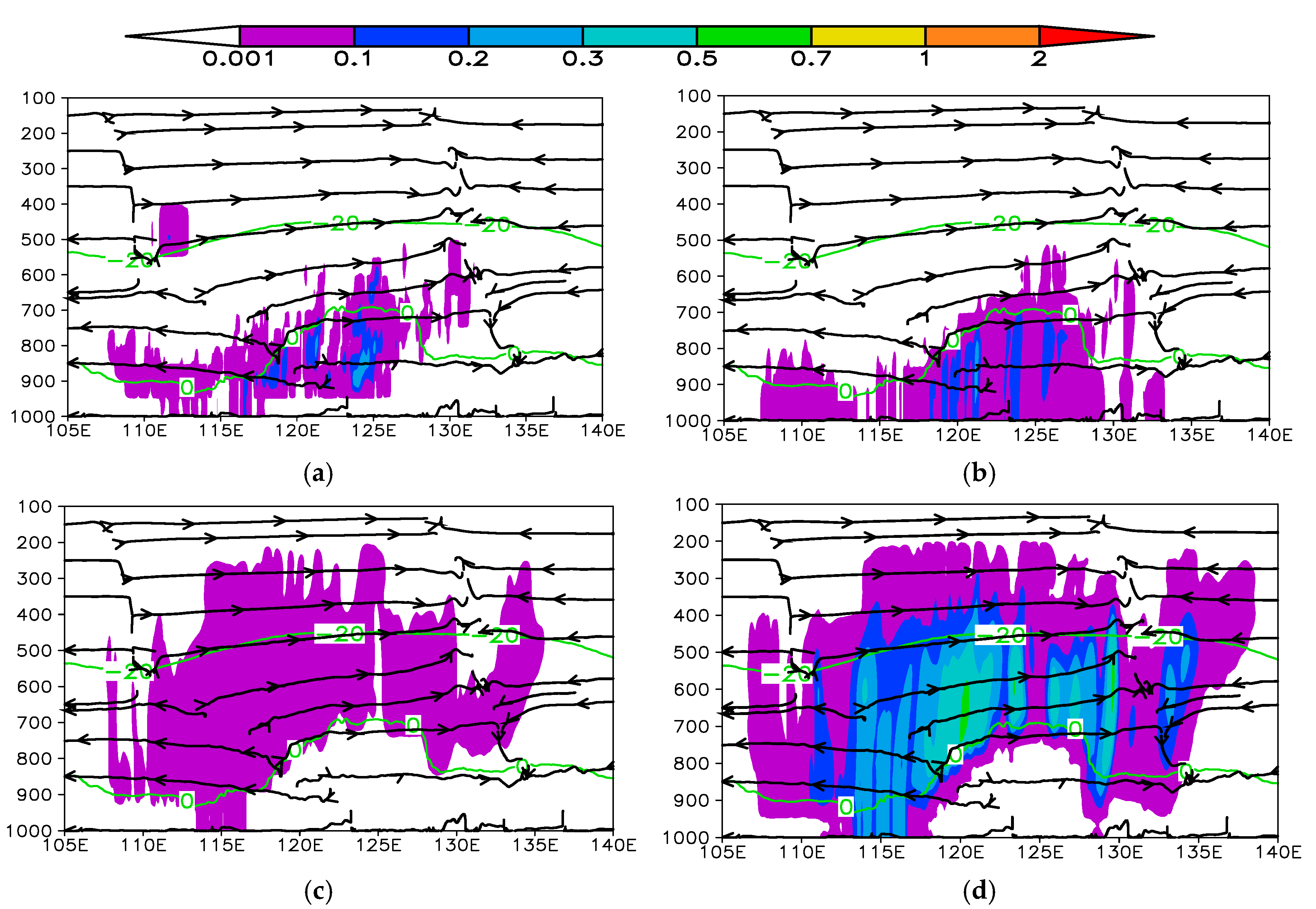
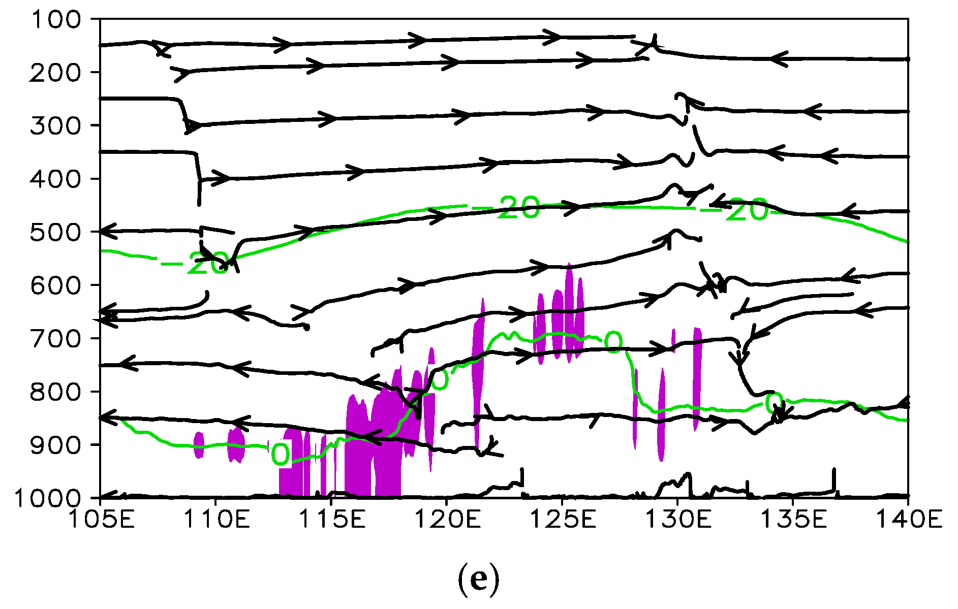
4.1.4. The Dissipation Period
The vortex cloud system rotated further; after 58 h of simulation, it split into two. The southeastern part of the system continued to move further towards the east, where it influenced northeast China and Korea.
Figure 4d shows the situation 67 h after the start of the simulation when the system split. During the movement, the system became weaker, with a maximum radar reflectivity of 15 dbz.
The hydrometeor mixing ratios in
Figure 8—i.e., the vertical distributions along the black line in
Figure 4d—show that the hydrometeor content in most of the cloud system was smaller than in the development and maintenance periods, while the cloud top descended from 200 hPa to 250–300 hPa, depending on the longitude.
Figure 8a,b shows the vertical profiles of the cloud and rain droplet mixing ratios, indicating that there were some areas with cloud droplets, with a maximum mixing ratio of only 0.2 g/kg. The rain mixing ratio was distributed at a very low level with a maximum of 0.3 g/kg. Less cloud and more rain meant that cloud coalescence did not produce sufficient rain. Most liquid precipitation was mainly due to the melting of snow.
During this period, there was no solid precipitation that reached the ground, as shown in
Figure 8c–e. The ice, snow and graupel contents peaked at 0.001, 0.7 and 0.001 g/kg, respectively. The solid particles covered most of the clouds, meaning that cold microphysical processes dominated and that precipitation was due to the melting of solid particles.
4.2. Microphysical Properties of the Northern Cloud Area
4.2.1. The Formation Period
The microphysical properties of the northern cloud system behaved quite differently from that in the southeast. The vertical cross-section of the hydrometeor mixing ratios during the formation period—i.e., along the black dashed line in
Figure 4a in the northern part of the cloud system—shows that it is a deep system with clouds extending as high as 300 hPa, as shown in
Figure 9a–e. During the formation stage, the simulation at 2 h after the start of the simulation shows that the system produced light solid and liquid precipitation with low radar reflectivity.
The mixing ratio of liquid particles inside or below the clouds was very small, as shown in
Figure 9a,b.
Figure 9a shows that the cloud droplets covered a very small area, with a maximum mixing ratio of only 0.001 g/kg. At the high latitudes of the northern clouds, the temperature was low, and so most cloud droplets were frozen and water vapor tended to be deposited onto solid particles. Besides, the cloud droplets were easily consumed by the Bergeron process or by accretion to solid particles. As a result, there were no rain droplets inside the cloud, as shown in
Figure 9b. Rain only existed below the clouds, with a maximum mixing ratio of 0.001 g/kg. Comparison with the snow mixing ratio distribution indicates that these rain droplets resulted from the melting of precipitating snow.
As shown in
Figure 9c–e, the clouds mainly consisted of solid particles, dominated by snow. The snow mixing ratio reached a maximum of 0.3 g/kg in the center of the cloud system; the maximum ice mixing ratio was 0.01 g/kg. Graupel covered only a small area below the clouds. The water vapor tended to be deposited onto solid particles; thus, there were sufficient ice and snow particles inside the clouds. The solid particles could grow through aggregation, accretion and the Bergeron process, but the contribution of accretion was small because there were insufficient cloud droplets, and thus there was hardly any graupel inside the clouds.
The dominance of the solid hydrometeors over the liquid droplets meant that the solid particles mainly grew through cold cloud processes and the precipitation consisted mainly of solid particles.
4.2.2. The Maintenance Period
The northern cloud band had no evident development period; therefore, only the maintenance period is discussed here. The vertical mixing ratios during this stage are presented in
Figure 10, at 48 h after the start of the simulation period. The clouds deepened and the cloud top extended as high as 200 hPa.
Figure 10a,b shows that, at this time, the cloud and rain droplets covered a much larger area inside and below the clouds than during the formation stage, with maximum mixing ratios of 0.2 and 0.1 g/kg, respectively. Some of the rain occurred at the same location as the cloud droplets; thus, some rain may have been caused by the coalescence of cloud droplets. However, because there were not many cloud particles, the coalescence process did not dominate the precipitation. At the same time, the cloud and rain centers were below the solid particles, where the temperature was higher than 0 °C, and so the rain was mainly caused by the melting of solid particles.
Figure 10c–e shows that solid hydrometeors were present at altitudes above the liquid droplets—in particular, between 118° E and 130° E—and these areas are separated by the −20 °C isotherm. The solid hydrometeors were dominated by snow, with a maximum mixing ratio of 0.5 g/kg. For ice and graupel, the maximum mixing ratio was 0.001 g/kg. There were many ice and snow particles due to deposition, aggregation and the Bergeron process. Graupel was formed along the freezing line in areas where the snow and liquid mixing ratios were high.
Precipitation mainly consisted of rain and snow, but generally not in the same area. In the area with the most intense snow, ice and graupel also occurred.
4.2.3. The Dissipation Period
After the vortex cloud system split into two, the northern cloud band moved further north and became weaker, but the cloud top height remained at about 200 hPa, as shown in
Figure 11a–e. The cloud water content in the dissipation period was smaller than before and produced a small amount of mixed liquid and solid precipitation.
As shown in
Figure 11a, the cloud droplets had a maximum mixing ratio of 0.1 g/kg.
Figure 11b shows that rain droplets mainly occurred below the clouds, which means that the rain was formed by the melting of solid particles. The distribution of solid particles was similar to that during the formation and maintenance periods (
Figure 11c–e). The snow particle content peaked at 0.3 g/kg, much higher than that of ice and graupel.
The cold cloud process dominated the precipitation and the surface precipitation consisted of snow, along with rain droplets formed by the melting of the solid particles.
5. Discussion
The evolution of the macro- and micro-physical properties of a cold vortex cloud system was studied as it progressed through different stages of development—formation, development, maintenance and dissipation—over four days. The system extended over an area nearly 5000 km long and 3500 km wide. During its movement, the vortex split into two centers, a northern and a southeastern system. The development of the macro- and micro-physical properties of both systems were simulated using the WRF model and the results were presented and discussed. The comparison of the macro-physical features with satellite and radar observations show a good agreement. However, this comparison could only be made over China. Although there are many weather stations and radar observatories in the study area, the base data for stations outside of China were not available for use in this study. Hence, the comparison was limited to only one satellite image and a radar product.
The focus of the study was on the microphysical properties and the processes during the different stages of the development of the cloud system. In the absence of radar station data or airborne microphysical observations, only model data could be presented. For the different stages of development of the two cloud systems, the mixing ratios of the six hydrometeor types were presented. The WRF model contains many options for physics and dynamics process, planetary boundary layer physics schemes, microphysics processes, cumulus parameterization schemes and radiation physics schemes. In the simulations, usually one scheme is selected for each of the processes, and in each scheme, many assumptions and parameters can be adjusted which are most appropriate for the purpose of the study. Obviously, the results of the study may be influenced by the choice of assumptions and parameters (see Gultepe et al. [
27] for a review of uncertainties).
6. Conclusions
(1) The macro- and micro-physical properties of a cloud system associated with a cold vortex system at 500 hPa, accompanied by a cold front and a warm front system at the surface level, were studied. The system lasted four days, from 0000 UTC on 20 May to 0000 UTC on 24 May, 2018. The cold vortex formed, strengthened, split into two and dissipated during the movement from west to east and triggered a large-scale cloud system and extensive precipitation.
(2) The precipitation was not evenly distributed. The liquid precipitation covered the whole area influenced by the cloud system, while the solid precipitation mainly covered areas north of 48° N. In the analyses, the cloud system was considered to consist of two parts: a southeastern part and a northern part.
(3) The liquid cloud and rain droplets covered only some smaller areas. There were insufficient liquid cloud droplets throughout most of the cloud system for the efficient production of rain droplets by coalescence. The rain droplets were mainly caused by the melting of solid particles precipitating out of the clouds, especially snow. The snow mixing ratio was largest, and ice and snow covered all of the cloud area, while only a small amount of graupel occurred in a small area. The reason for the distribution of the solid particles was that they could grow through aggregation, the Bergeron process or accretion, which produced many snow particles, while there were insufficient liquid particles to support the formation of very large particles such as graupel. When precipitating out of the clouds, some solid particles melted and produced liquid rain droplets, while some remained solid. Cold cloud processes dominated the microphysical processes in the system.
(4) The southeastern cloud part influenced a larger area and mainly produced liquid precipitation, with solid precipitation mainly occurring north of 48° N. The northern cloud system influenced a smaller area and produced mainly mixed precipitation. The liquid precipitation was mainly rain that formed from the melting of solid particles. The solid precipitation consisted mainly of snow precipitating out of clouds and not melting, along with some graupel.
(5) The work presents a case study of rainfall from a cold vortex system and studied the microphysical features and precipitation mechanism of the system. Further simulation studies and field experiments are planned to study these phenomena.


