Late-Spring Severe Blizzard Events over Eastern Romania: A Conceptual Model of Development


Abstract
:1. Introduction
2. Data and Methods
3. Results—Case Study
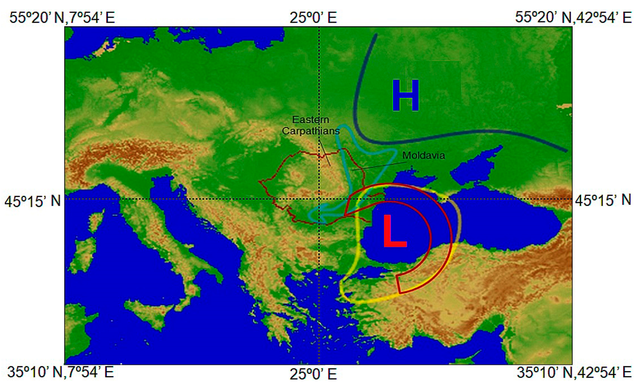
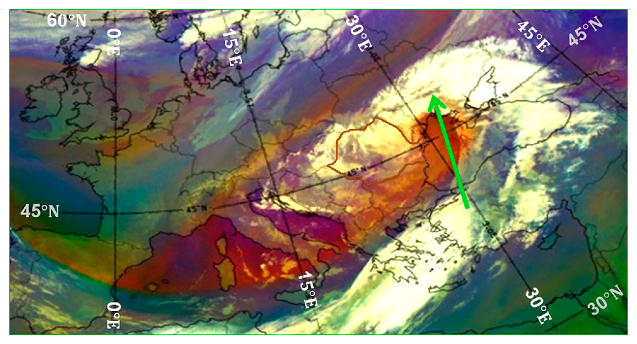
3.1. Observed Synoptic Context
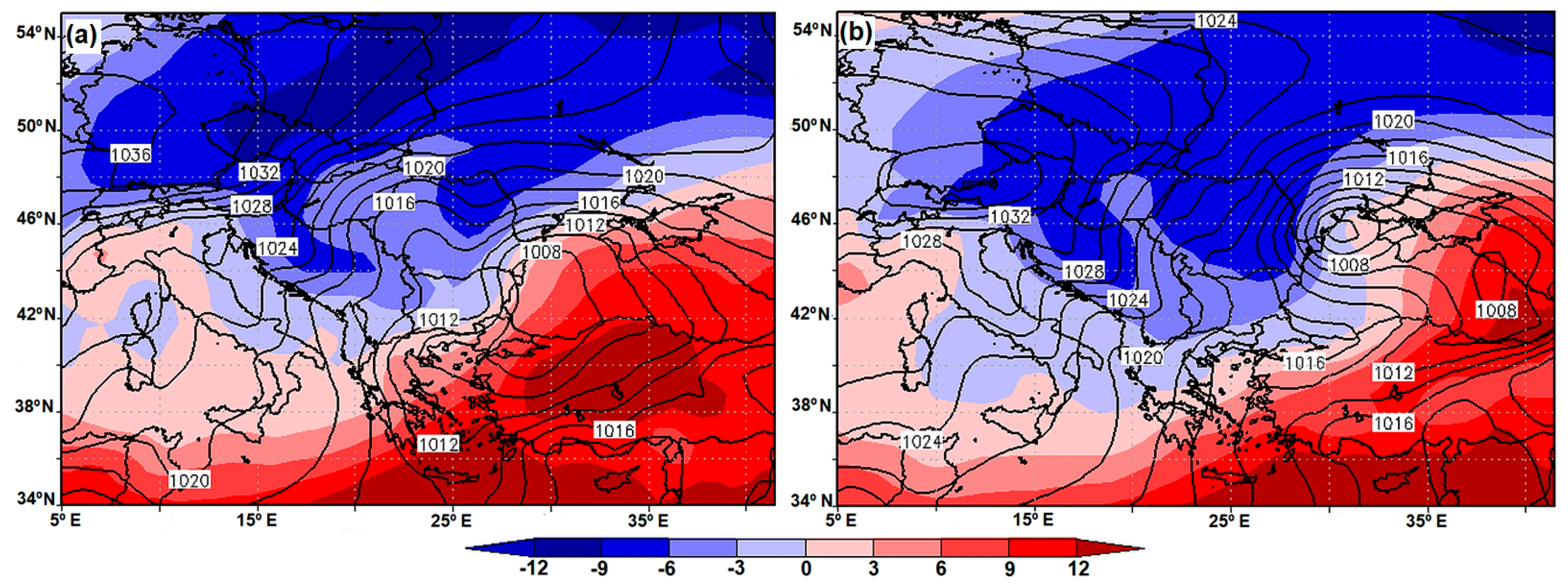
3.2. Numerical Simulations
3.2.1. Large-Scale Forcing
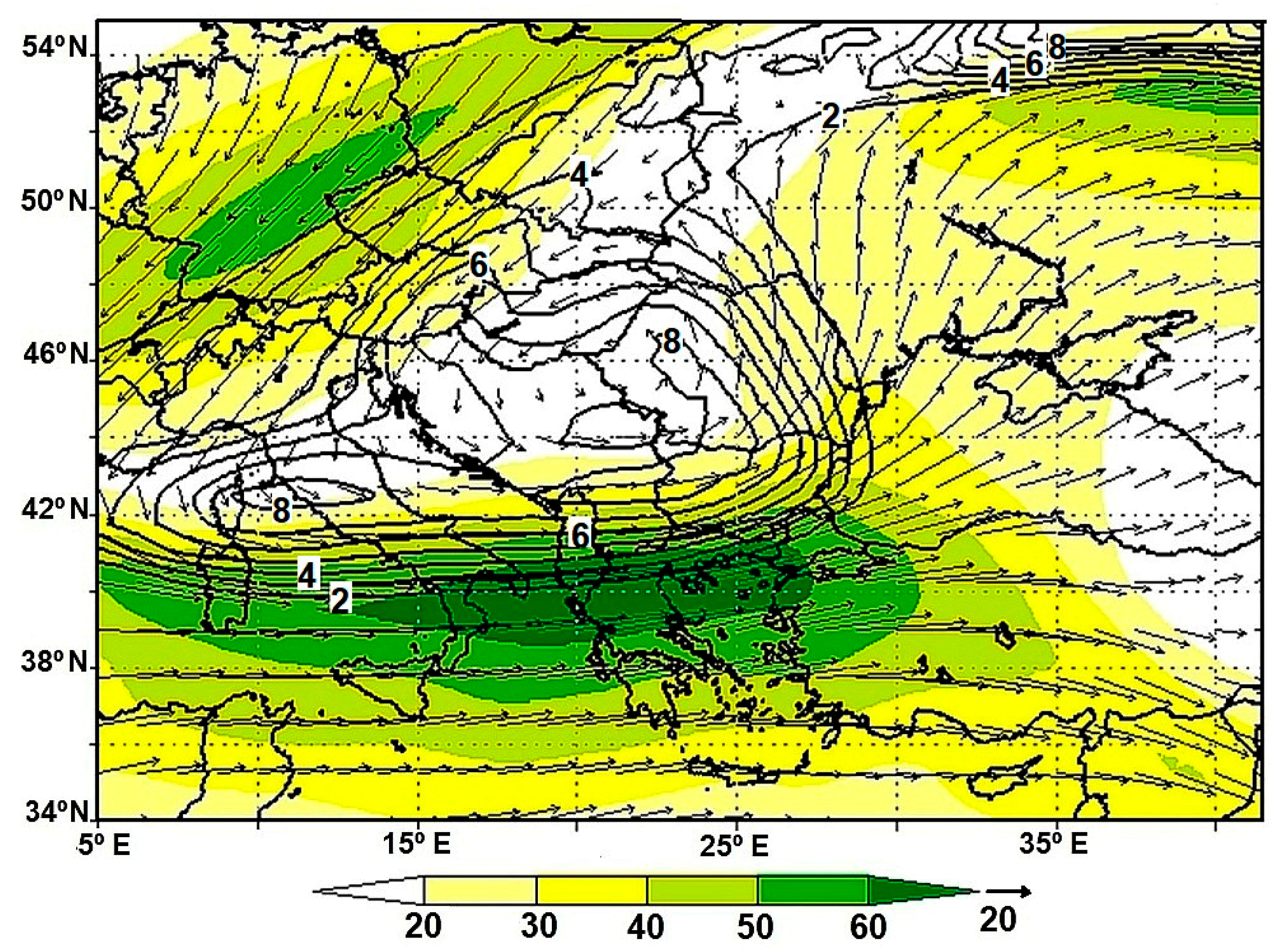
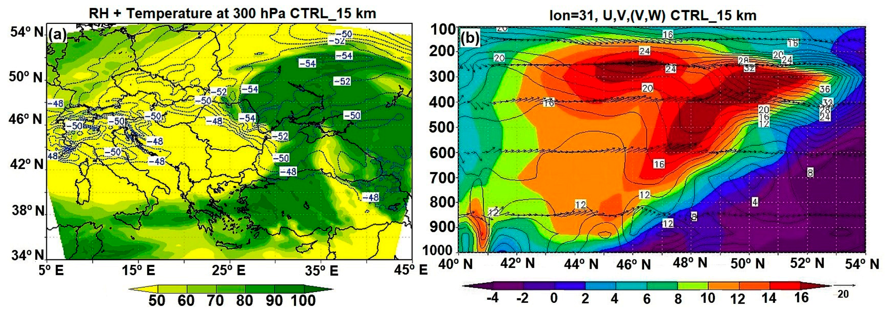
The Upper-Level Jet (ULJ)
Large-Scale Humidity–Temperature Advection from the Mediterranean Sea
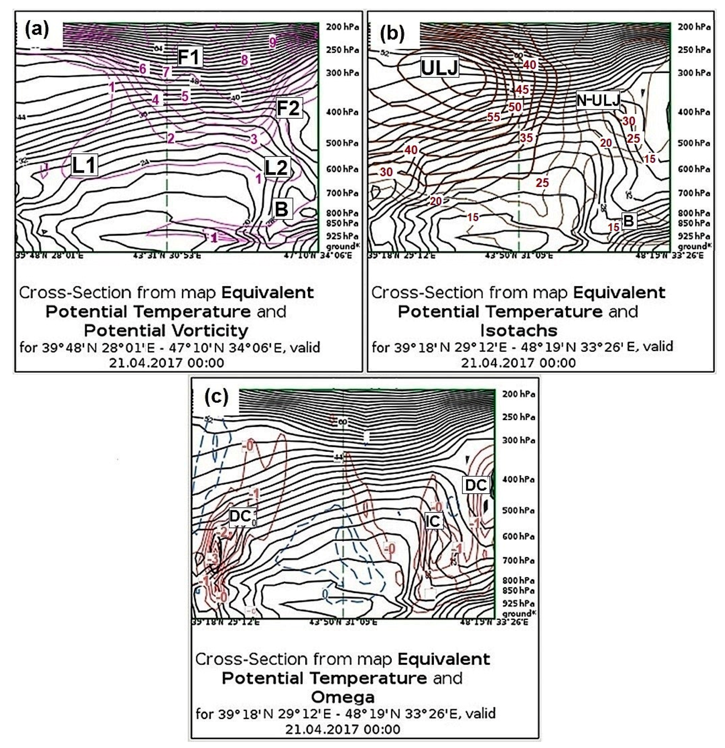
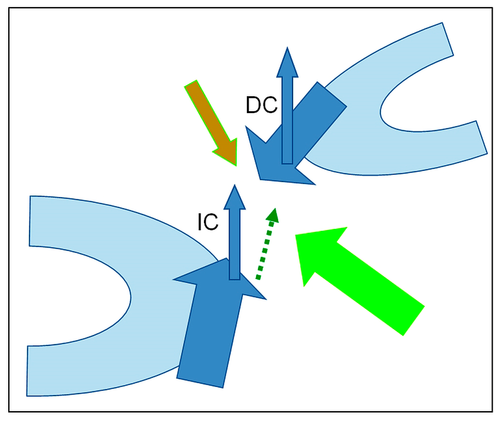
3.2.2. Large–Regional Scale Interaction: An Enhancing Mechanism
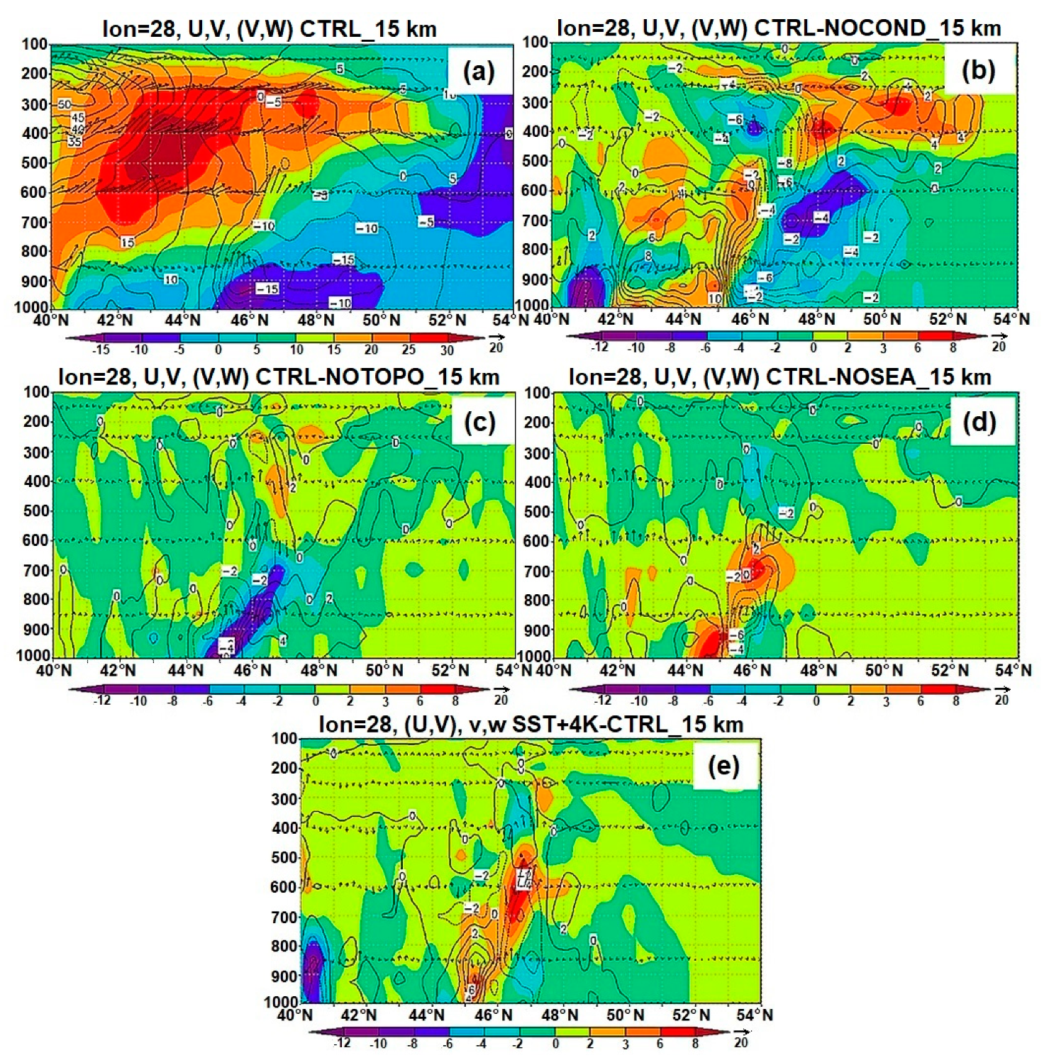
LLJs (Low-Level Jets)
Baroclinicity and Ageostrophic Circulations
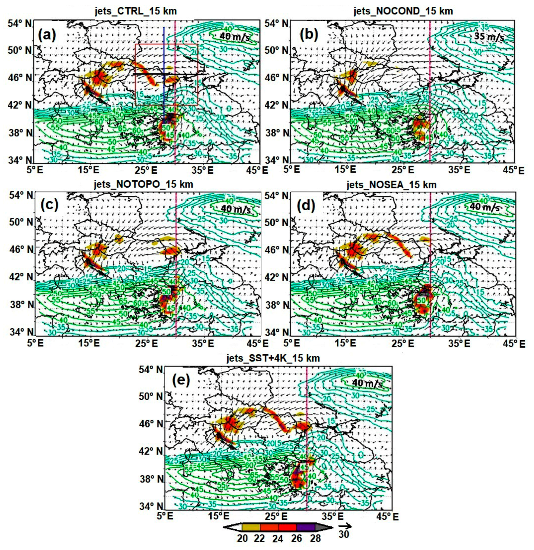
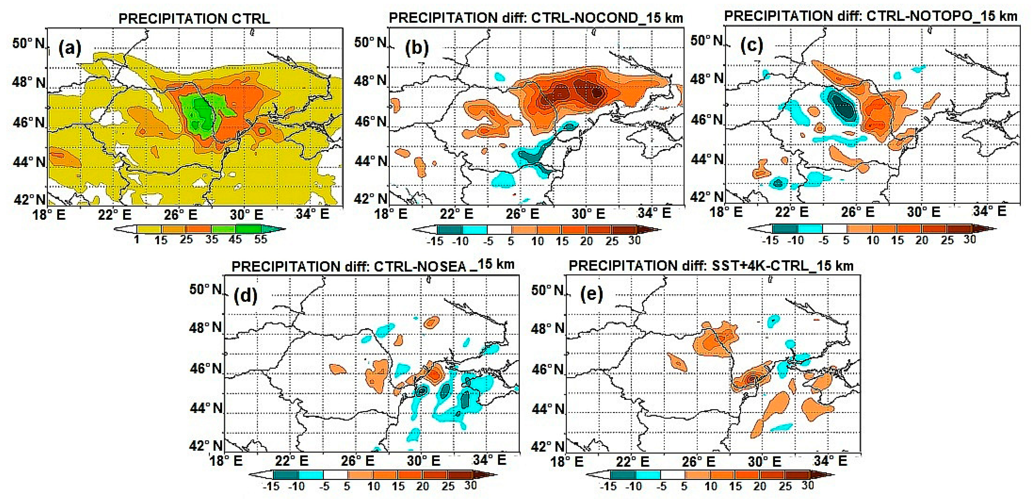
3.2.3. Regional Forcings: Role on Localization and Development of the Event
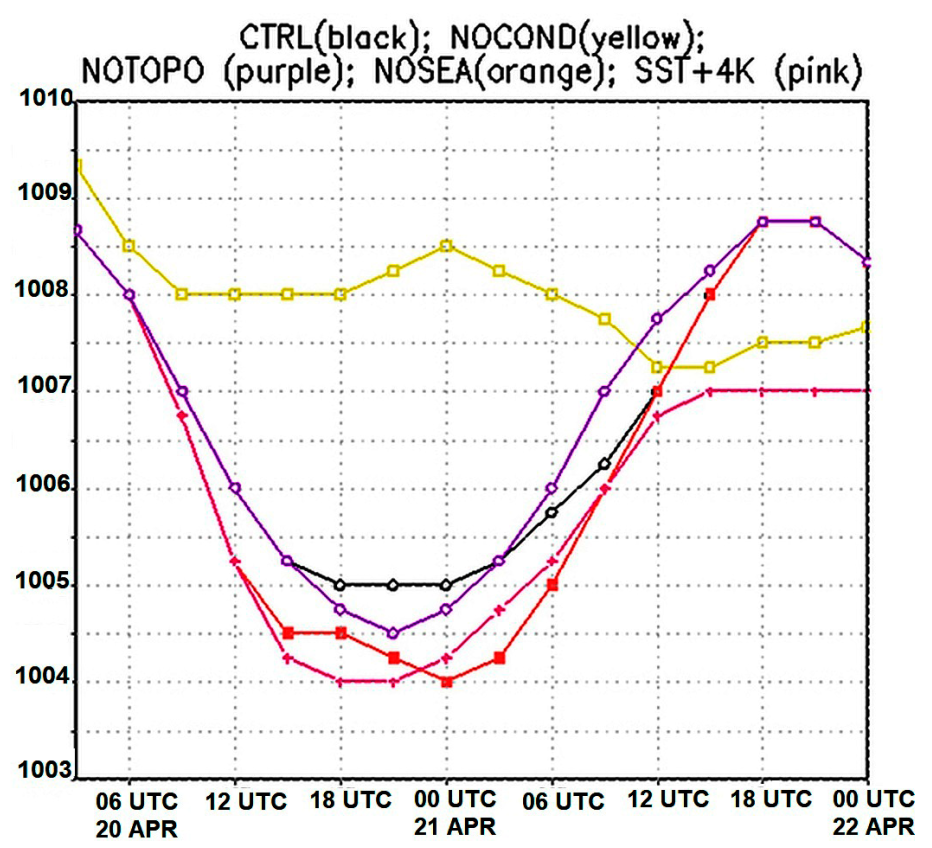
Deepening
Persistence
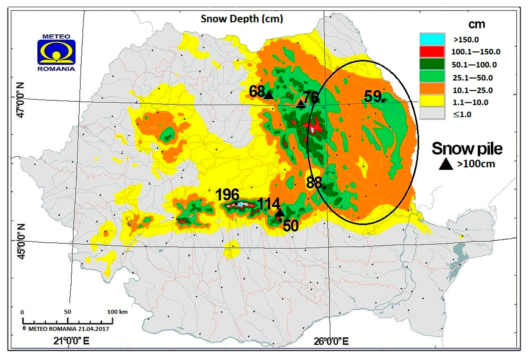
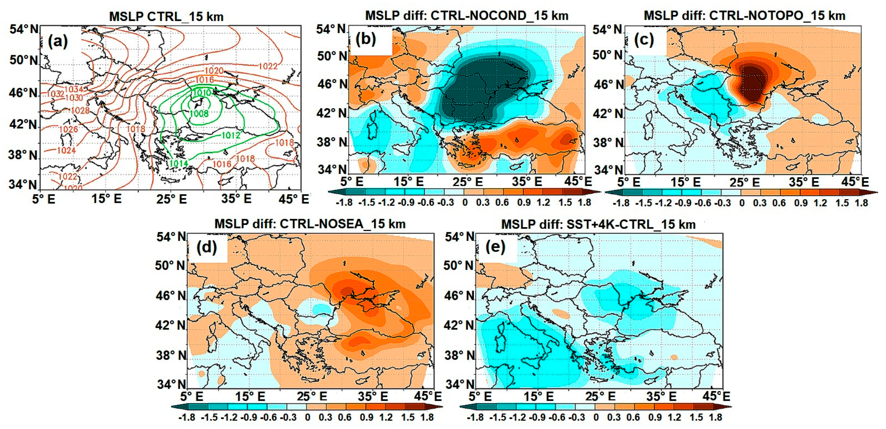
Location and Extent
Sea and SST
Condensation and Surface Fluxes
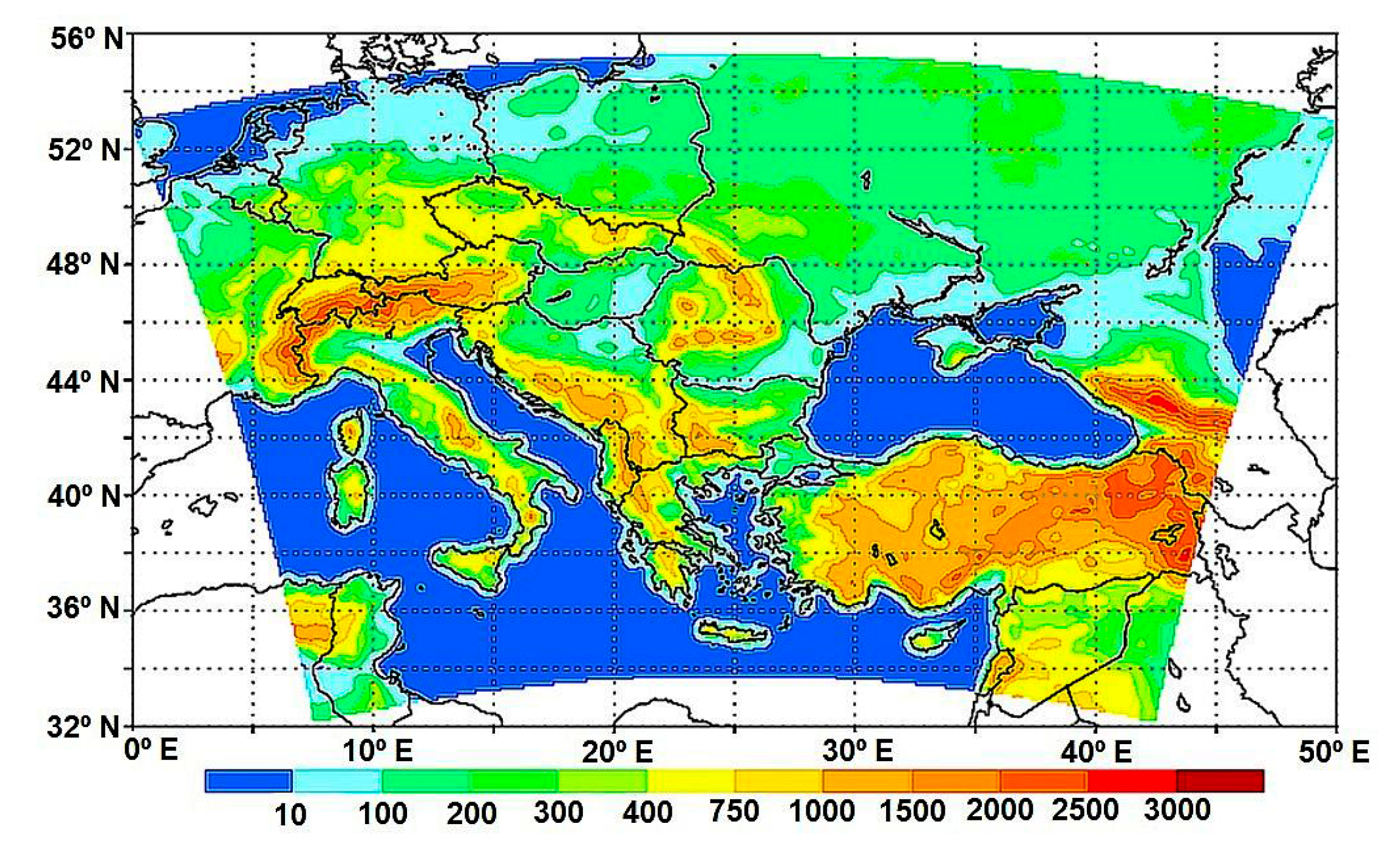
Topography
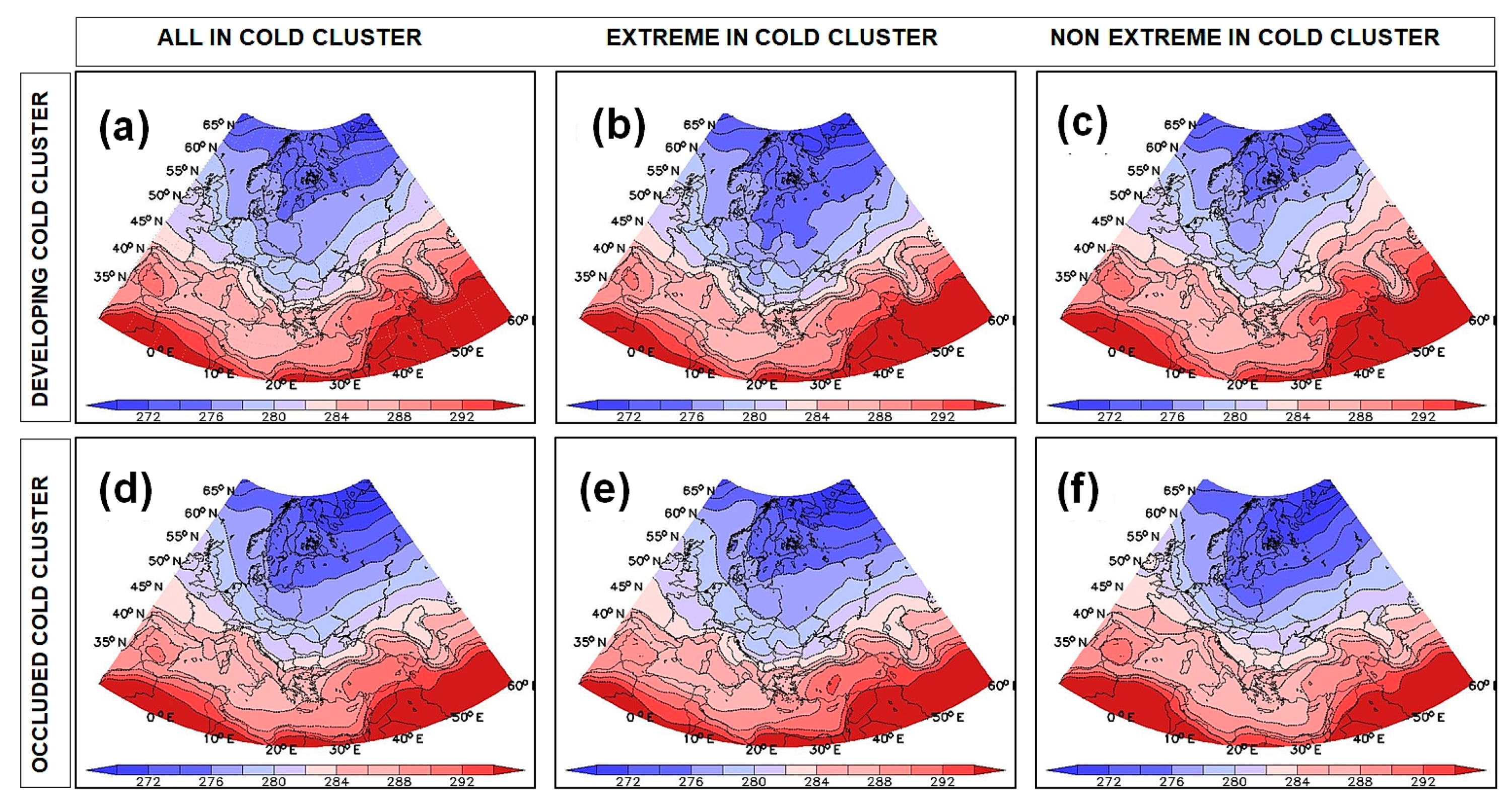
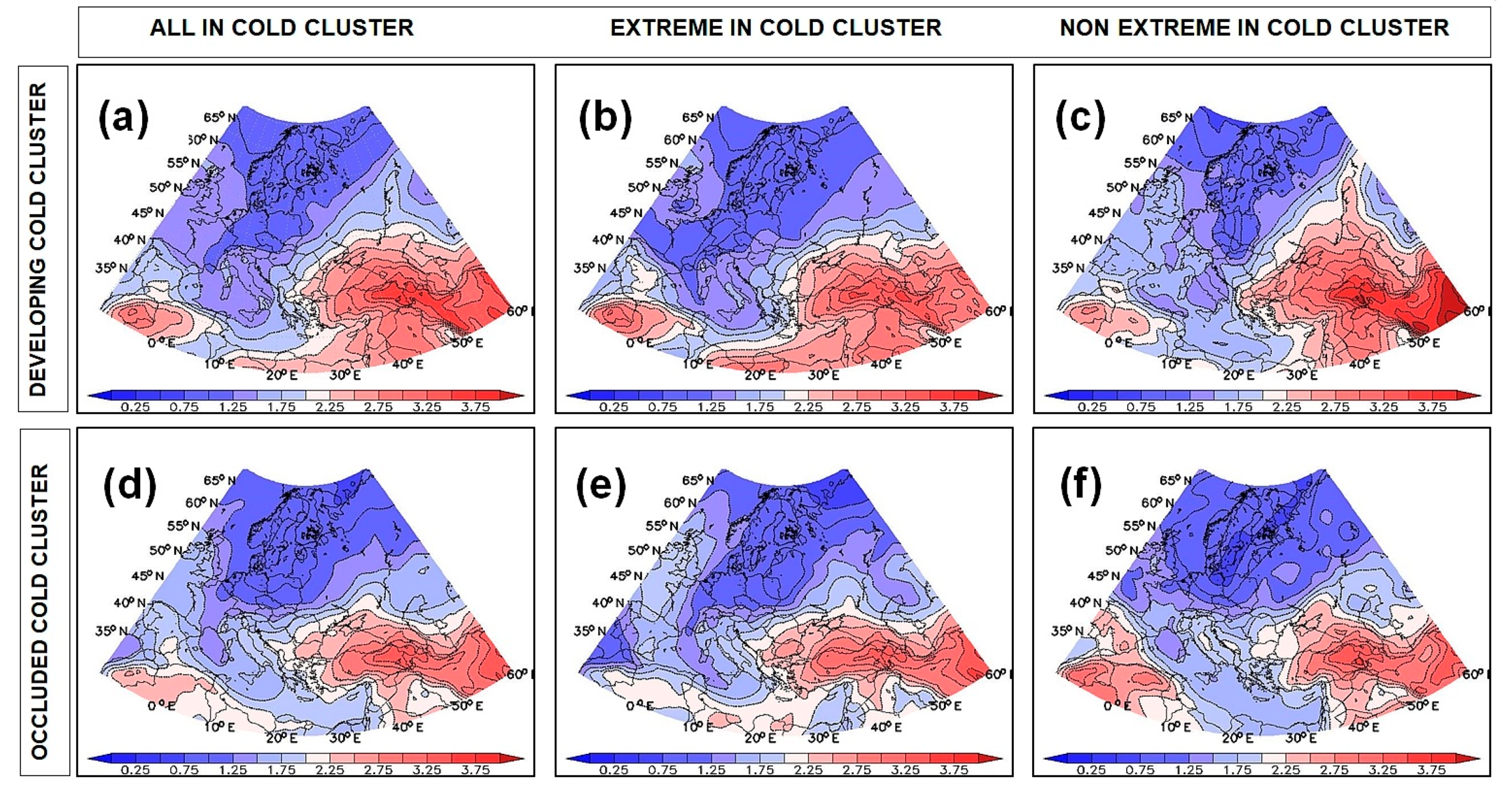
4. Event Climatology and Mechanism Validation over 40 Years
4.1. The Conceptual Model
4.2. The Mechanism Validation
5. Conclusions
Author Contributions
Funding
Acknowledgments
Conflicts of Interest
References
- Cazacioc, L. Spatial and Temporal Variability of Extreme Daily Precipitation Amounts in Romania. Rom. J. Meteorol. 2007, 9, 34–46. [Google Scholar]
- Apostol, L. The Mediterranean Cyclones–the Role in Ensuring Water Resources and Their Potential of Climatic Risk, in the East of Romania. Present Environ. Sustain. Dev. 2008, 2, 143–163. [Google Scholar]
- Vespremeanu-Stroe, A.; Cheval, S.; Tatui, F. The Wind Regime of Romania-Characteristics, Trends and North Atlantic Oscillation Influences/Regimul Vânturilor Din România-Caracteristici, Tendinte Si Influentele Oscilatiilor Nord-Atlantice. In Forum Geografic: Studii si Cercetari de Geografie si Protectia Mediului; University of Craiova, Department of Geography: Craiova, Romania, 2012; Volume 11, pp. 116–118. [Google Scholar]
- Stefanescu, V.; Stefan, S.; Georgescu, F. Spatial Distribution of Heavy Precipitation Events in Romania between 1980 and 2009. Meteorol. Appl. 2014, 21, 684–694. [Google Scholar] [CrossRef]
- Hustiu, M.C. The Risk of Blizzard Appearing in Barlad Plateau during 1981–2010. Revista Riscuri Si Catastrofe 2017, 20. [Google Scholar] [CrossRef]
- Brâncuş, M.; Schultz, D.M.; Antonescu, B.; Dearden, C.; Ştefan, S. Origin of Strong Winds in an Explosive Mediterranean Extratropical Cyclone. Mon. Weather Rev. 2019, 147, 3649–3671. [Google Scholar] [CrossRef]
- Trigo, I.F.; Bigg, G.R.; Davies, T.D. Climatology of Cyclogenesis Mechanisms in the Mediterranean. Mon. Weather Rev. 2002, 130, 549–569. [Google Scholar] [CrossRef]
- Ion-Bordei, N.; Ion-Bordei, E. Fenomene Meteoclimatice Induse de Configuraţia Carpaţilor în Câmpia Română; Editura Academiei Române: Bucharest, Romania, 2008. [Google Scholar]
- Georgescu, F.; Stefan, S. Cyclonic Activity over Romania in Connection with the Air Circulation Types. Rom. Rep. Phys. 2010, 62, 878–886. [Google Scholar]
- Surkova, G.; Arkhipkin, V.; Kislov, A. Atmospheric Circulation and Storm Events in the Black Sea and Caspian Sea. Open Geosci. 2013, 5, 548–559. [Google Scholar] [CrossRef]
- Georgescu, F.; Tascu, S.; Caian, M.; Banciu, D. A Severe Blizzard Event in Romania–A Case Study. Nat. Hazards Earth Syst. Sci. 2009, 9, 623–634. [Google Scholar] [CrossRef] [Green Version]
- Ion-Bordei, E. Rolul Lanţului Alpino-Carpatic În Evoluţia Ciclonilor Mediteraneeni; Editura Printech: Bucharest, Romania, 2009. [Google Scholar]
- Drăghici, I. Dinamica Atmosferei; Editura Tehnică: Bucharest, Romania, 1988. [Google Scholar]
- Popa, F.; Soci, C. Méthode Classique et Actuelle d’analyse d’une Tempête de Neige. Revue Roumaine de Geographie 2002, 45, 77–186. [Google Scholar]
- Cordoneanu, E. Particularităţi Ale Dinamicii Aerului Deasupra României; Editura Fundaţiei “România de Mâine”: Bucharest, Romania, 2009. [Google Scholar]
- Georgescu, M. The First Severe Blizzard Episode of December 2009. Rom. J. Meteorol. 2010, 10, 13. [Google Scholar]
- Danciu-Ciurlãu, D. An Episode of Late Blizzard, 25-26 March 2013. Present Environ. Sustain. Dev. 2014, 8, 165–174. [Google Scholar] [CrossRef] [Green Version]
- Sandu, I.; Pescaru, V.; Poiana, I. Clima Romaniei; Editura Academiei Romane: Bucuresti, Romania, 2008. [Google Scholar]
- Bălescu, O.I.; Beşleagă, N.N. Viscolele În Republica Populară Română; Institutul Meteorlogic: Bucharest, Romania, 1962. [Google Scholar]
- Ciurlău, D. Climatological Landmarks of the Blizzard Phenomenon in the Bărăgan Plain Area. Aerul Si Apa Compon. Ale Mediu. 2014, 1, 461–468. [Google Scholar]
- Manta, R.; Sfîcă, L.; Tişcovschi, A.; Constantin, D.; Mănoiu, V.; Radu, C. Late Snowfall and Blizzards in Moldavia, April 2017. Summary, Case of Study. Aerul. Si Apa Compon. Ale Mediu. 2018, 61–68. [Google Scholar] [CrossRef]
- Bogdan, O.; Marinică, I. Hazarde Meteo-Climatice Din Zona Temperată: Factori Genetici şi Vulnerabilitate: Aplicaţii La România; Editura Universităţii “Lucian Blaga”: Sibiu, Romania, 2007. [Google Scholar]
- Bojan, D. The Blizzard in the Zarand Land. Analele Univ. Din Oradea Ser. Geogr. 2008, 18, 81–85. [Google Scholar]
- Costache, R.; Fontanine, I. The Snow Drift Potential in the Plain Area of Buzău County. Analele Univ. Din Oradea Ser. Geogr. 2013, 23, 245–254. [Google Scholar]
- Manta, D.; Hustiu, M.; Sipos, Z. Agravating Factors in the Blizzard Situations in the South-East of Romania. Aerul Si Apa Compon. Ale Mediu. 2015, 446. [Google Scholar] [CrossRef]
- Uccellini, L.W.; Kocin, P.J. The Interaction of Jet Streak Circulations during Heavy Snow Events along the East Coast of the United States. Weather 1987, 2, 289–308. [Google Scholar] [CrossRef] [Green Version]
- Kumar, A.; Zhang, L.; Wang, W. Sea Surface Temperature–Precipitation Relationship in Different Reanalyses. Mon. Weather Rev. 2013, 141, 1118–1123. [Google Scholar] [CrossRef] [Green Version]
- Dado, J.M.B.; Takahashi, H.G. Potential Impact of Sea Surface Temperature on Rainfall over the Western Philippines. Prog. Earth Planet. Sci. 2017, 4, 23. [Google Scholar] [CrossRef] [Green Version]
- Llasat, M.-C.; Rigo, T.; Montes, J.-M. Orographic Role in the Temporal and Spatial Distribution of Precipitation. The Case of the Internal Basins of Catalonia (Spain). In Proceedings of the EGS Plinius Conference, Maratea, Italy, 14–16 October 1999; pp. 41–55. [Google Scholar]
- Muhammad Tahir, K.; Yin, Y.; Wang, Y.; Babar, Z.A.; Yan, D. Impact Assessment of Orography on the Extreme Precipitation Event of July 2010 over Pakistan: A Numerical Study. Adv. Meteorol. 2015, 2015. [Google Scholar] [CrossRef]
- Twardosz, R.; Cebulska, M.; Walanus, A. Anomalously Heavy Monthly and Seasonal Precipitation in the Polish Carpathian Mountains and Their Foreland during the Years 1881–2010. Appl. Clim. 2016, 126, 323–337. [Google Scholar] [CrossRef] [Green Version]
- Dee, D.P.; Uppala, S.; Simmons, A.; Berrisford, P.; Poli, P.; Kobayashi, S.; Andrae, U.; Balmaseda, M.; Balsamo, G.; Bauer, D.P. The ERA-Interim Reanalysis: Configuration and Performance of the Data Assimilation System. Q. J. R. Meteorol. Soc. 2011, 137, 553–597. [Google Scholar] [CrossRef]
- Giorgi, F.; Anyah, R. The Road towards RegCM4. Clim. Res. 2012, 52, 3–6. [Google Scholar] [CrossRef] [Green Version]
- Elguindi, N.; Bi, X.; Giorgi, F.; Nagarajan, B.; Pal, J.; Solmon, F.; Rauscher, S.; Zakey, A.; O’Brien, T.; Nogherotto, R. Regional Climate Model RegCM: Reference Manual Version 4.5; Abdus Salam ICTP Trieste: Trieste, Italy, 2014. [Google Scholar]
- Stoelinga, M.T. A Potential Vorticity-Based Study of the Role of Diabatic Heating and Friction in a Numerically Simulated Baroclinic Cyclone. Mon. Weather Rev. 1996, 124, 849–874. [Google Scholar] [CrossRef] [Green Version]
- Romero, R.; Ramis, C.; Alonso, S. Numerical Simulation of an Extreme Rainfall Event in Catalonia: Role of Orography and Evaporation from the Sea. Q. J. R. Meteorol. Soc. 1997, 123, 537–559. [Google Scholar] [CrossRef]
- Ahmadi-Givi, F.; Graig, G.; Plant, R. The Dynamics of a Midlatitude Cyclone with Very Strong Latent-heat Release. Q. J. R. Meteorol. Soc. 2004, 130, 295–323. [Google Scholar] [CrossRef] [Green Version]
- Horvath, K.; Fita, L.; Romero, R.; Ivancan-Picek, B. A Numerical Study of the First Phase of a Deep Mediterranean Cyclone: Cyclogenesis in the Lee of the Atlas Mountains. Meteorol. Z. 2006, 15, 133–146. [Google Scholar] [CrossRef] [Green Version]
- Persson, P.O.G.; Hare, J.; Nance, L.; Walter, B. Impact of Air-Sea Interaction on Extra-Tropical Cyclones. In Proceedings of the ECMWF Workshop on Ocean-Atmosphere Interactions, Berkshire, UK, 10–12 November 2008; pp. 123–146. [Google Scholar]
- Pastor, F.; Gómez, I.; Estrela, M. Numerical Study of the October 2007 Flash Flood in the Valencia Region (Eastern Spain): The Role of Orography. Nat. Hazards Earth Syst. Sci. 2010, 10, 1331. [Google Scholar] [CrossRef] [Green Version]
- Messmer, M.; Gómez-Navarro, J.; Raible, C. Sensitivity Experiments on the Response of Vb Cyclones to Sea Surface Temperature and Soil Moisture Changes. Earth Syst. Dyn. 2017, 8, 477–493. [Google Scholar] [CrossRef] [Green Version]
- Kim, K.-Y.; Lee, S.; Kim, M.-K.; Cho, C.-H. Long-Term Variability of Cold Surges in Korea. Asia-Pac. J. Atmos. Sci. 2014, 50, 519–529. [Google Scholar] [CrossRef]
- Park, T.-W.; Ho, C.-H.; Jeong, J.-H.; Heo, J.-W.; Deng, Y. A New Dynamical Index for Classification of Cold Surge Types over East Asia. Clim. Dyn. 2015, 45, 2469–2484. [Google Scholar] [CrossRef]
- Lensky, I.; Rosenfeld, D. Clouds-Aerosols-Precipitation Satellite Analysis Tool (CAPSAT). Atmos. Chem. Phys. 2008, 8, 6739–6753. [Google Scholar] [CrossRef] [Green Version]
- Hoskins, B.J.; McIntyre, M.E.; Robertson, A.W. On the Use and Significance of Isentropic Potential Vorticity Maps. Q. J. R. Meteorol. Soc. 1985, 111, 877–946. [Google Scholar] [CrossRef]
- Lackmann, G. Midlatitude Synoptic Meteorology, Cdr Edition; American Meteorological Society: Boston, MA, USA, 2011. [Google Scholar]
- Martin, J.E. Mid-Latitude Atmospheric Dynamics: A First Course; John Wiley & Sons: Hoboken, NJ, USA, 2013. [Google Scholar]
- Vaughan, G.; Antonescu, B.; Schultz, D.M.; Dearden, C. Invigoration and Capping of a Convective Rainband Ahead of a Potential Vorticity Anomaly. Mon. Weather Rev. 2017, 145, 2093–2117. [Google Scholar] [CrossRef]
- Henri, C. Device for Deflecting a Stream of Elastic Fluid Projected into an Elastic Fluid. U.S. Patent No. 2,052,869, 1 September 1936. [Google Scholar]
- Munson, B.R.; Young, D.F.; Okiishi, T.H. Instructor’s Manual to Accompany Fundamentals of Fluid Mechanics; Wiley: Hoboken, NJ, USA, 1990. [Google Scholar]
- Georgiev, C.G.; Santurette, P. Mid-Level Jet in Intense Convective Environment as Seen in the 7.3 m Satellite Imagery. Atmos. Res. 2009, 93, 277–285. [Google Scholar] [CrossRef]
- Wernli, H.; Dirren, S.; Liniger, M.A.; Zillig, M. Dynamical Aspects of the Life Cycle of the Winter Storm ‘Lothar’ (24–26 December 1999). Q. J. R. Meteorol. Soc. 2002, 128, 405–429. [Google Scholar] [CrossRef]
- Agustí-Panareda, A.; Thorncroft, C.; Craig, G.; Gray, S. The Extratropical Transition of Hurricane Irene: A Potential-vorticity Perspective. Q. J. R. Meteorol. Soc. 2004, 130, 1047–1074. [Google Scholar] [CrossRef]
- Flocas, H.A.; Simmonds, I.; Kouroutzoglou, J.; Keay, K.; Hatzaki, M.; Bricolas, V.; Asimakopoulos, D. On Cyclonic Tracks over the Eastern Mediterranean. J. Clim. 2010, 23, 5243–5257. [Google Scholar] [CrossRef]


| Scale | Triggers | |
|---|---|---|
| Large Scale | * upper-level jet (ULJ) | |
| * moisture advection (q adv) | ||
| Large–Regional Scale Interactions | * low-level jets (LLJs): southerly (linked to indirect ageostrophic circulation (IC) and q adv); northerly (linked to direct ageostrophic circulation (DC) and topography) * baroclinicity * ageostrophic circulations | |
| Regional Scale | Regional Triggers | Sensitivity Numerical Experiment |
| * Black Sea | experiment: NOSEA | |
| * sea surface temperature (SST) anomaly | experiment: SST + 4 k | |
| * topography | experiment: NOTOPO | |
| * condensation | experiment: NOCOND | |
| Cyclone Type | Impact Type | ||
|---|---|---|---|
| Cold (32) | Developing (17) | Extreme (9) | Non-extreme (8) |
| Occluding (15) | Extreme (8) | Non-extreme (7) | |
| Warm (48) | Unstratified | ||
© 2019 by the authors. Licensee MDPI, Basel, Switzerland. This article is an open access article distributed under the terms and conditions of the Creative Commons Attribution (CC BY) license (http://creativecommons.org/licenses/by/4.0/).
Share and Cite
Caian, M.; Andrei, M.D. Late-Spring Severe Blizzard Events over Eastern Romania: A Conceptual Model of Development. Atmosphere 2019, 10, 770. https://doi.org/10.3390/atmos10120770
Caian M, Andrei MD. Late-Spring Severe Blizzard Events over Eastern Romania: A Conceptual Model of Development. Atmosphere. 2019; 10(12):770. https://doi.org/10.3390/atmos10120770
Chicago/Turabian StyleCaian, Mihaela, and Meda Daniela Andrei. 2019. "Late-Spring Severe Blizzard Events over Eastern Romania: A Conceptual Model of Development" Atmosphere 10, no. 12: 770. https://doi.org/10.3390/atmos10120770