Unprecedented Rainfall and Moisture Patterns during El Niño 2016 in the Eastern Pacific and Tropical Andes: Northern Perú and Ecuador


Abstract
:1. Introduction
2. Data and Methodology
2.1. Precipitation
2.2. Moisture Transport
2.3. EOF/PC Analysis on C and E Indices
3. Results
3.1. The EOF Modes of , its Convergence (), and Rainfall Variability
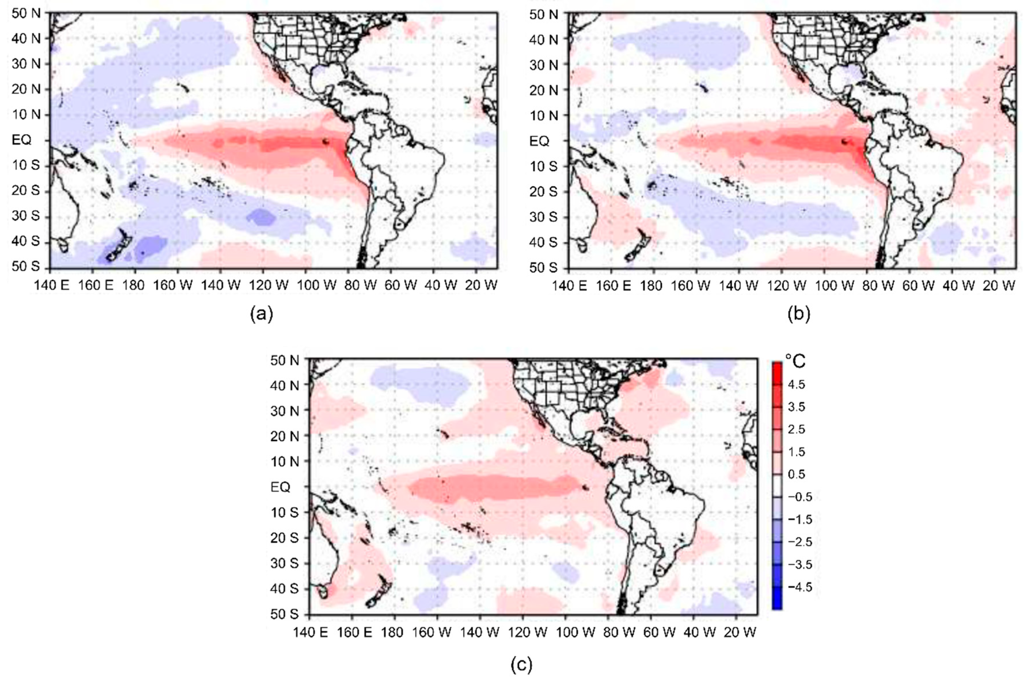
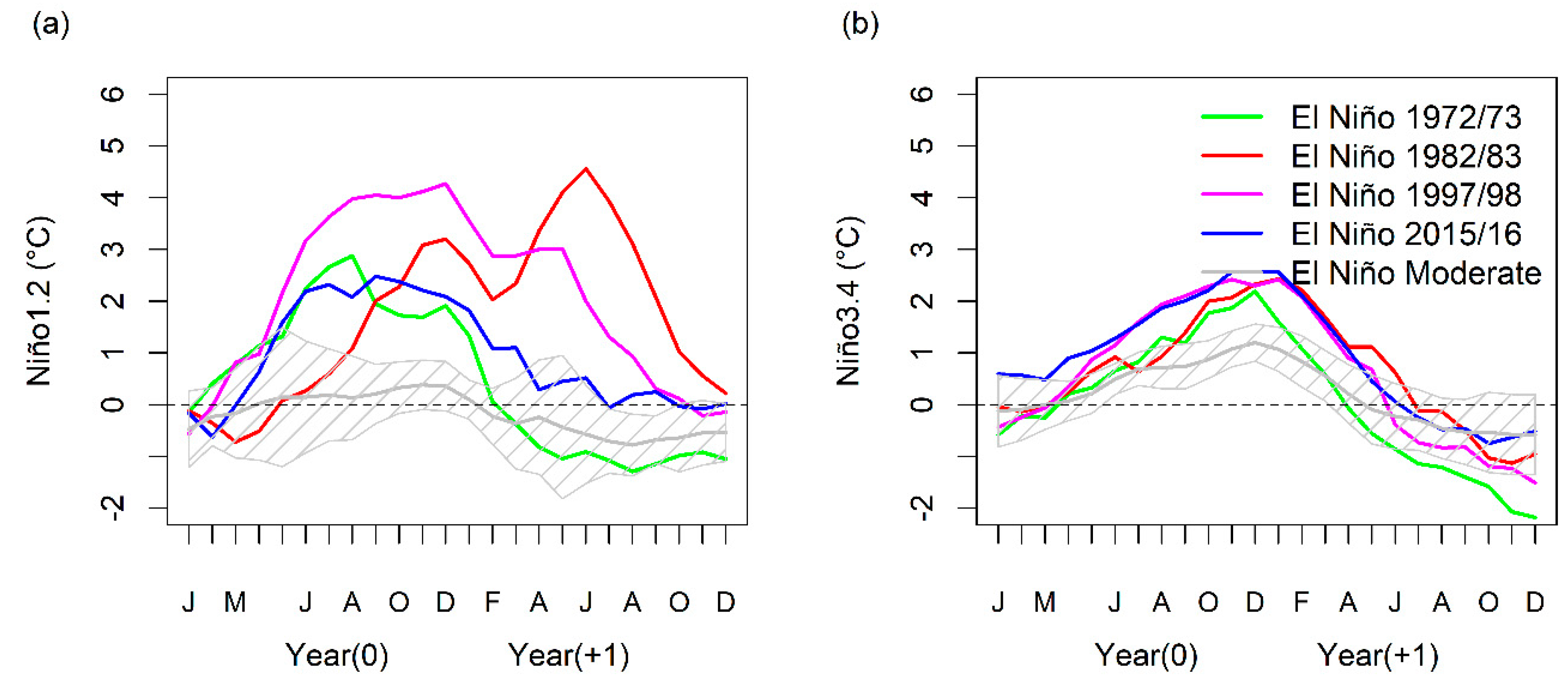
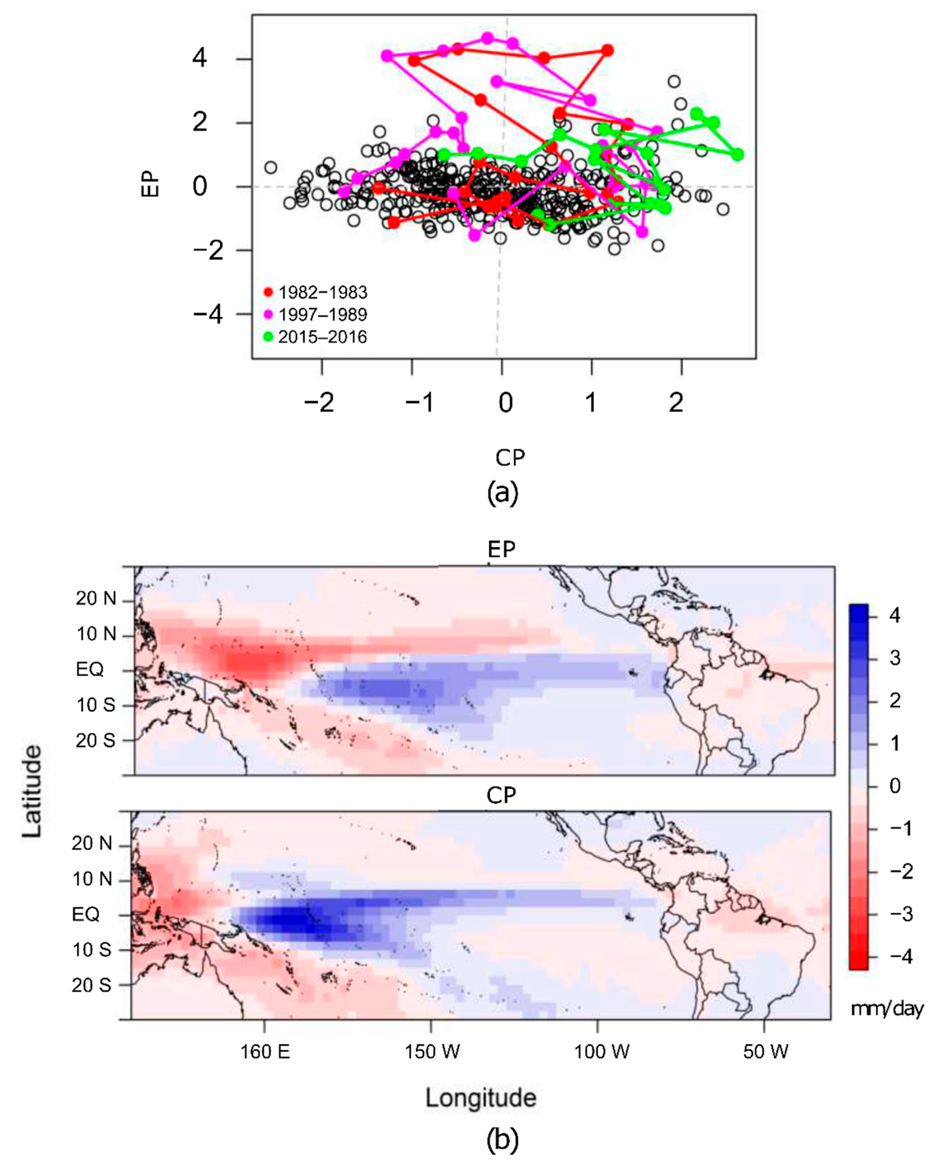
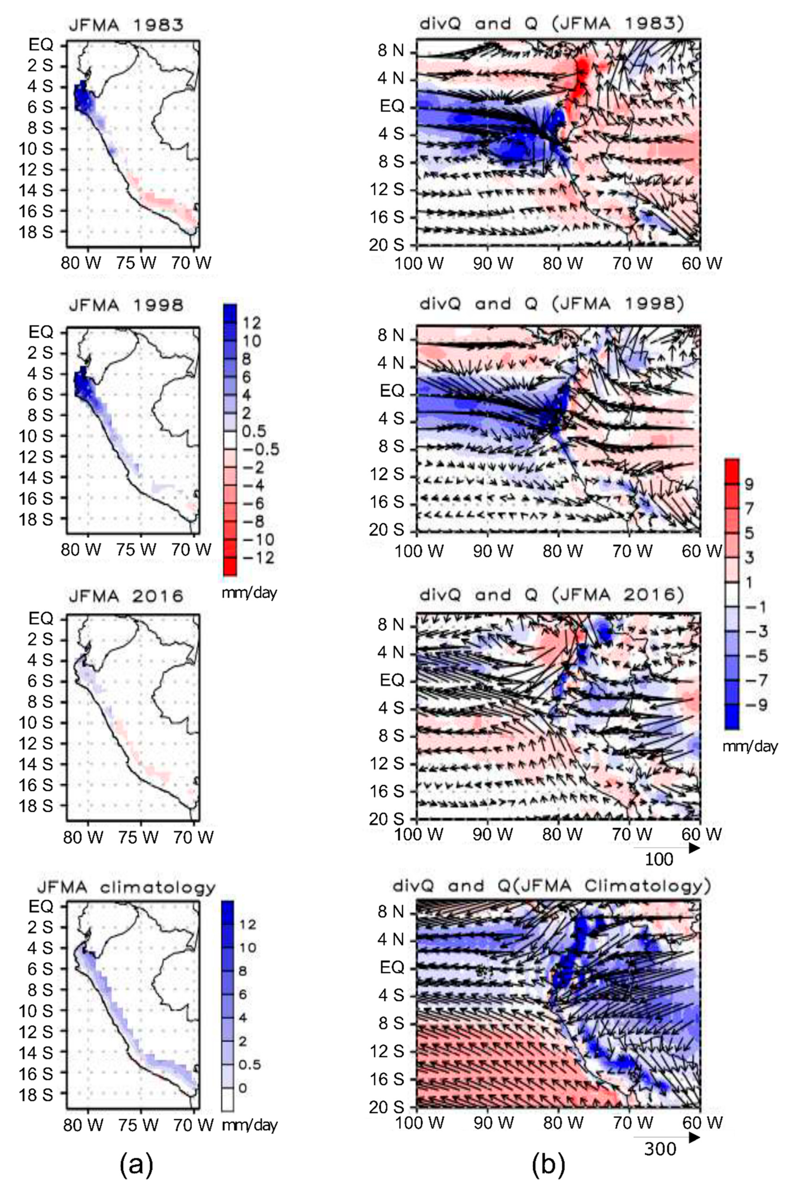
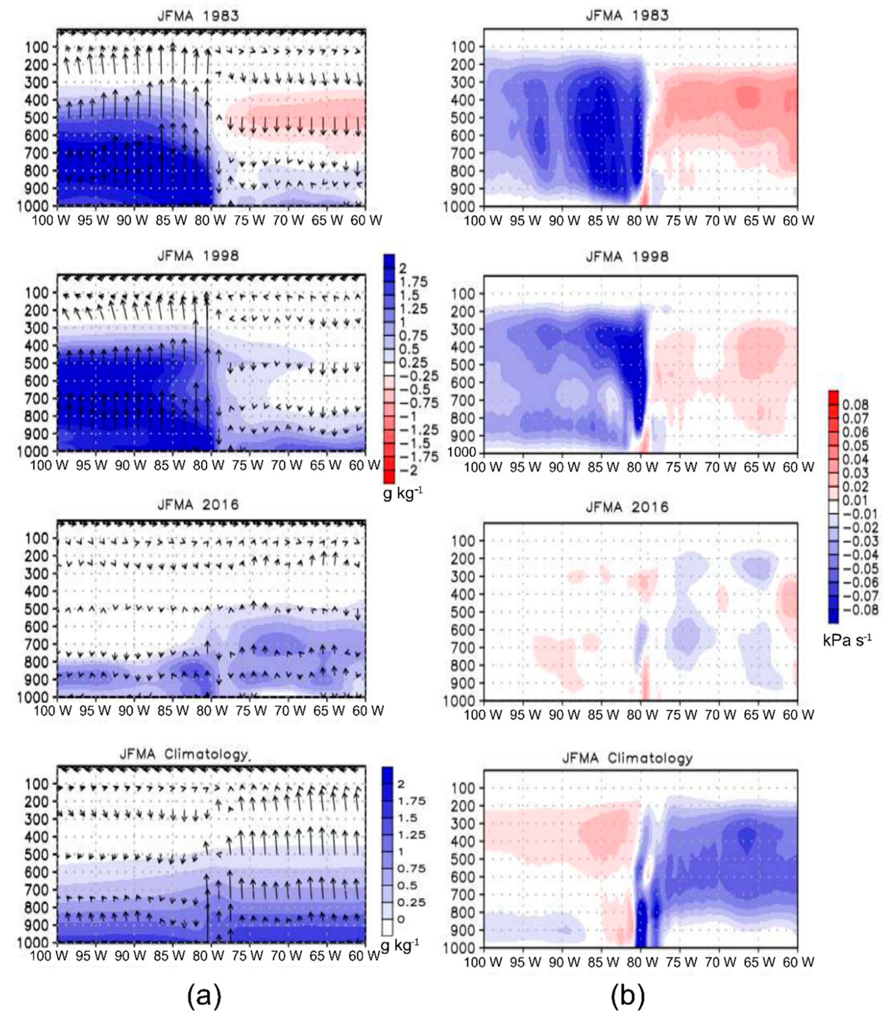
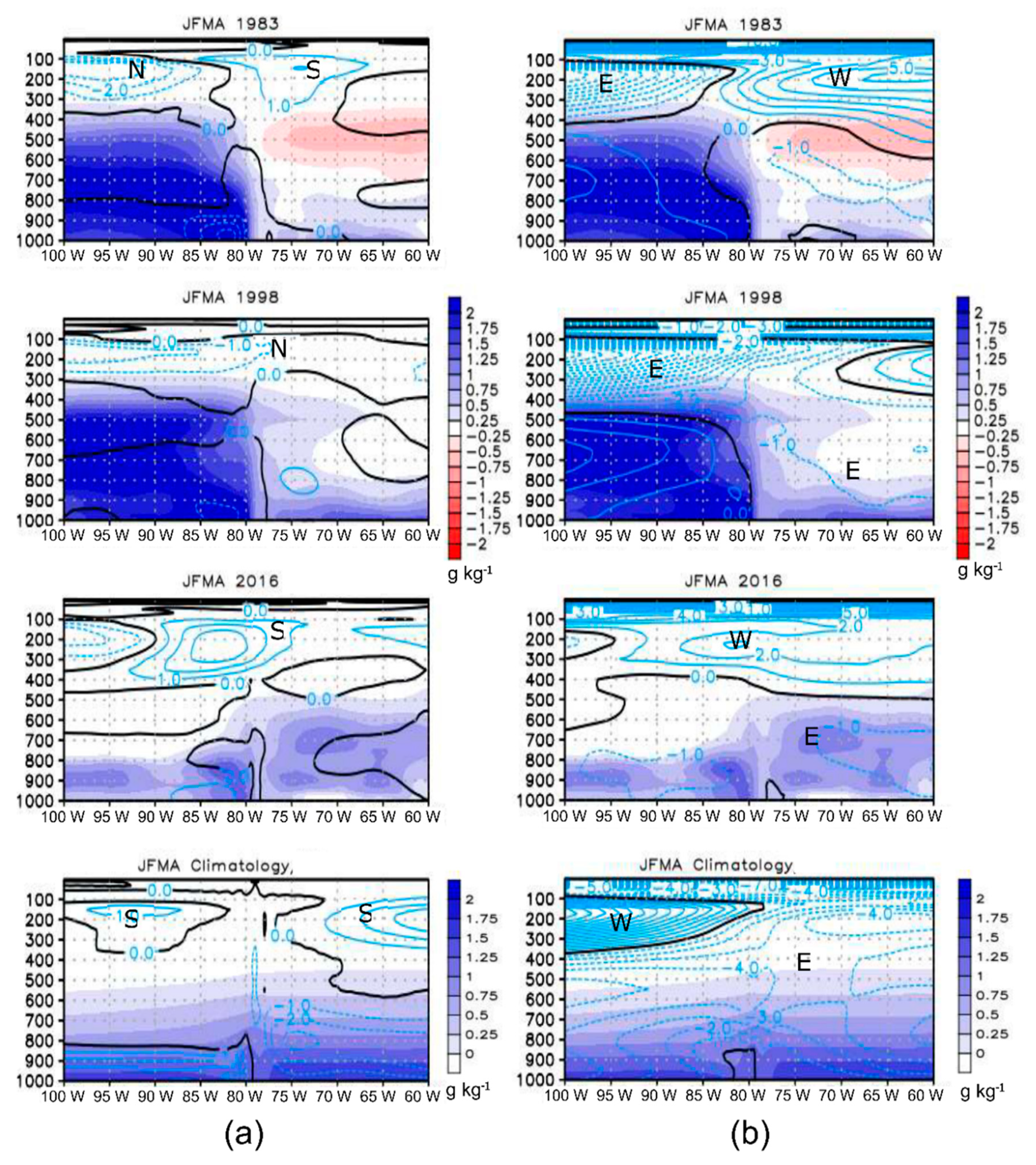
3.2. Observed Rainfall, , and during Strong El Niño Events
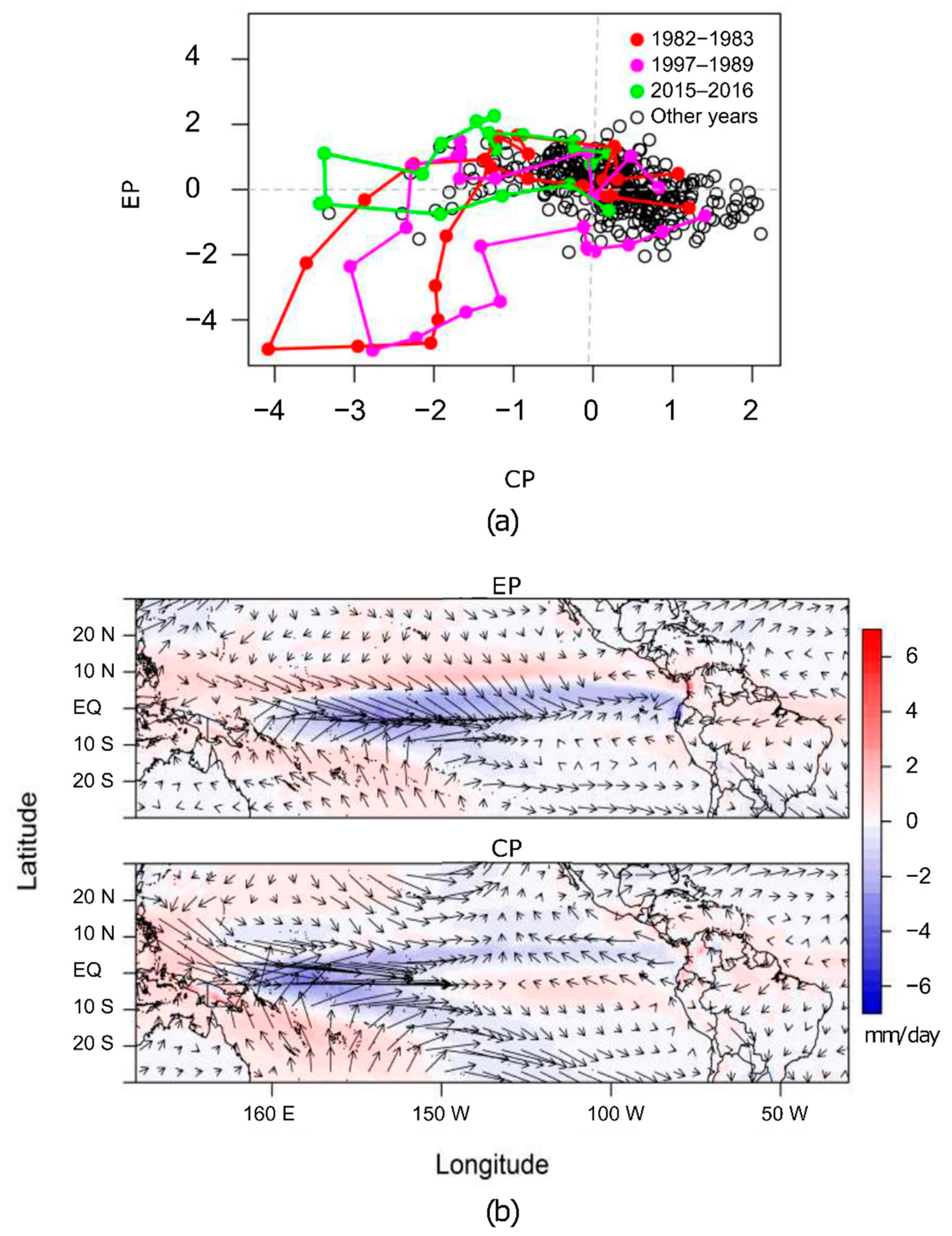
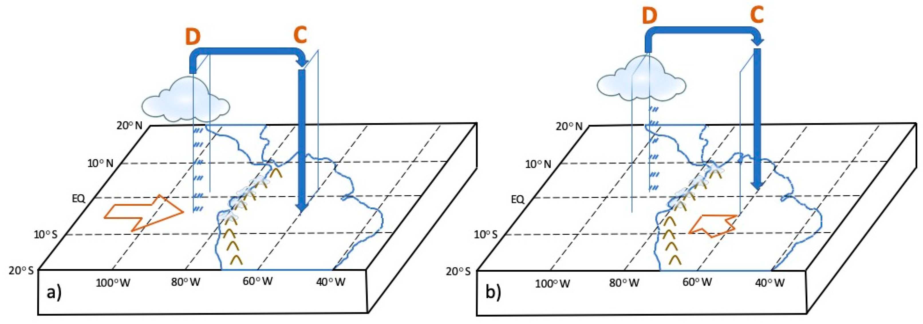
3.3. Global and Regional Driving Mechanisms
4. Conclusions
Supplementary Materials
Author Contributions
Funding
Acknowledgments
Conflicts of Interest
References
- Bjerknes, J. Atmospheric teleconnections from the equatorial Pacific. Mon. Weather Rev. 1969, 97, 163–172. [Google Scholar] [CrossRef]
- Rasmusson, E.M.; Carpenter, T.H. Variations in tropical sea surface temperature and surface wind fields associated with the Southern Oscillation/El Niño. Mon. Weather Rev. 1982, 110, 354–384. [Google Scholar] [CrossRef]
- Deser, C.; Wallace, J.M. El Niño events and their relation to the Southern Oscillation: 1925–1986. J. Geophys. Res. 1987, 92, 14189–14196. [Google Scholar] [CrossRef]
- Davey, M.K.; Brookshaw, A.; Ineson, S. The probability of the impact of ENSO on precipitation and near-surface temperature. Clim. Risk Manag. 2014, 1, 5–24. [Google Scholar] [CrossRef] [Green Version]
- McPhaden, M.J.; Zebiak, S.E.; Glantz, M.H. ENSO as an integrating concept in Earth science. Science 2006, 314, 1740–1745. [Google Scholar] [CrossRef] [PubMed] [Green Version]
- Ropelewski, C.H.; Halpert, S. Global and regional scale precipitation patterns associated with the El Nin˜o/Southern Os- cillation. Mon. Weather Rev. 1987, 115, 1606–1626. [Google Scholar] [CrossRef] [Green Version]
- Quiroz, R.S. The climate of the “El Niño” winter of 1982-83—A season of extraordinary climatic anomalies. Mon. Weather Rev. 1983, 111, 1685–1706. [Google Scholar] [CrossRef] [Green Version]
- Barnett, T.P. Interaction of the monsoon and Pacific trade wind system at interannual time scales. Part III: A partial anatomy of the Sourthen Oscillation. Mon. Weather Rev. 1984, 112, 2388–2400. [Google Scholar] [CrossRef] [Green Version]
- Horel, J.D.; Cornejo-Garrido, A.G. Convection along the coast of northern Peru during 1983: Special and temporal variation of clouds and rainfall. Mon. Weather Rev. 1986, 114, 2091–2105. [Google Scholar] [CrossRef] [Green Version]
- Goldberg, R.A.; Tisnado, G.M.; Scofield, R.A. Characteristics of extreme rainfall events in northwestern Peru during the 1982–1983 El Nino period. Geophys. Res. Lett. 1987, 92, 14225–14241. [Google Scholar] [CrossRef]
- Takahashi, K. The atmospheric circulation associated with extreme rainfall events in Piura, Peru, during the 1997–1998 and 2002 El Niño events. Ann. Geophys. 2004, 22, 3917–3926. [Google Scholar] [CrossRef] [Green Version]
- Bourrel, L.; Rau, P.; Dewitte, B.; Labat, D.; Lavado, W.; Coutaud, A.; Vera, A.; Alvarado, A.; Ordoñez, J. Low-frequency modulation and trend of the relationship between ENSO and precipitation along the northern to centre Peruvian Pacific coast. Hydrol. Process. 2016, 29, 1252–1266. [Google Scholar] [CrossRef]
- Sanabria, J.; Bourrel, L.; Dewitte, B.; Frappart, F.; Rau, P.; Soils, O.; David, L. Rainfall along the coast of Peru during strong El Niño events. Int. J. Climatol. 2018, 38. [Google Scholar] [CrossRef]
- Sulca, J.; Takahashi, K.; Espinoza, J.; Vuille, M.; Lavado, W. Impacts of ENSO flavors and tropical Pacific convection variability (ITCZ, SPCZ) on austral summer rainfall in South America focused on Peru. Int. J. Clim. 2017. [Google Scholar] [CrossRef]
- Morata, C.R.; Ballesteros, J.A.; Rohrer, M.; Stoffel, M. The anomalous 2017 coastal El Niño event in Peru. Clim. Dyn. 2018. [Google Scholar] [CrossRef]
- Garreaud, R.D. Short Communication A plausible atmospheric trigger for the 2017 coastal El Niño. Int. J. Climatol. 2018, 38, e1296–e1302. [Google Scholar] [CrossRef]
- Garreaud, R.D. Intraseasonal variability of moisture and rainfall over the South American Altiplano. Mon. Weather Rev. 2000, 128, 3337–3346. [Google Scholar] [CrossRef] [Green Version]
- Eichler, T.P.; Londoño, A.C. South American climatology and impacts of El Niño in NCEP’s CFSR data. Adv. Meteorol. 2013, 2013. [Google Scholar] [CrossRef]
- Pineda, L.; Ntegeka, V.; Willems, P. Rainfall variability related to sea surface temperature anomalies in a Pacific-Andean basin into Ecuador and Peru. Adv. Geosci. 2013, 33, 53–62. [Google Scholar] [CrossRef] [Green Version]
- Gimeno, L.; Dominguez, F.; Nieto, R.; Trigo, R.; Drumond, A.; Reason, C.J.C.; Kumar, R.; Marengo, J. Major Mechanisms of Atmospheric Moisture Transport and their Role in Extreme Precipitation Events. Annu. Rev. Environ. Resour. 2016, 41, 117–141. [Google Scholar] [CrossRef] [Green Version]
- Garreaud, R.D. The Andes climate and weather. Adv. Geosci. 2009, 7, 1–9. [Google Scholar] [CrossRef] [Green Version]
- Kao, H.Y.; Yu, J.Y. Contrasting Eastern-Pacific and Central-Pacific types of ENSO. J. Clim. 2009, 22, 615–632. [Google Scholar] [CrossRef]
- Takahashi, K.; Montecinos, A.; Goubanova, K.; Dewitte, B. ENSO regimes: Reinterpreting the canonical and Modoki El Nio. Geophys. Res. Lett. 2011. [Google Scholar] [CrossRef] [Green Version]
- Capotondi, A.; Wittenberg, A.T.; Newman, M.; Di Lorenzo, E.; Yu, J.-Y.; Braconnot, P.; Cole, J.; Dewitte, B.; Giese, B.; Guilyardi, E.; et al. Understanding ENSO diversity. Bull. Am. Meteorol. Soc. 2015, 96, 921–938. [Google Scholar] [CrossRef]
- Vecchi, G.A. The termination of the 1997-98 El Niño. Part II: Mechanisms of atmospheric change. J. Clim. 2006, 19, 2647–2664. [Google Scholar] [CrossRef] [Green Version]
- Takahashi, K.; Battisti, D.S. Processes controlling the mean tropical Pacific precipitation pattern. Part II: The SPCZ and the Southeast Pacific dry zone. J. Clim. 2007, 20, 5696–5706. [Google Scholar] [CrossRef]
- Tedeschi, R.G.; Cavalcanti, I.F.A.; Grimm, A.M. Influences of two types of ENSO on South American precipitation. Int. J. Climatol. 2013, 33, 1382–1400. [Google Scholar] [CrossRef]
- Waliser, D.E.; Gautier, C. A satellite-derived climatology of the ITCZ. J. Clim. 1993, 6, 2162–2174. [Google Scholar] [CrossRef]
- L’Heureux, M.L.; Takahashi, K.; Watkins, A.B.; Barnston, A.G.; Becker, E.J.; Di Liberto, T.E.; Gamble, F.; Gottschalck, J.; Halpert, M.S.; Huang, B.; et al. Observing and Predicting the 2015-16 El Niño. Bull. Amer. Meteorol. Soc. 2016. [Google Scholar] [CrossRef]
- Levine, A.F.Z.; McPhaden, M.J. How the July 2014 easterly wind burst gave the 2015-2016 El Niño a head start. Geophys. Res. Lett. 2016, 43, 6503–6651. [Google Scholar] [CrossRef]
- Paek, H.Y.; Qian, J.-Y.C. Why were the 2015/16 and 1997/98 Extreme El Niños different? Geophys. Res. Lett. 2017, 44, 1848–1856. [Google Scholar] [CrossRef]
- Hu, S.; Fedorov, A.V. The extreme El Niño of 2015–2016: The role of westerly and easterly wind bursts, and preconditioning by the failed 2014 event. Clim. Dyn. 2017, 1–19. [Google Scholar] [CrossRef]
- Paixao Veiga, J.A.; Rao, V.B.; Franchito, S.H. Heat and moisture budgets of the walker circulation and associated rainfall anomalies during El Niño events. Int. J. Climatol. 2005, 25, 193–213. [Google Scholar] [CrossRef]
- Rau, P.; Bourrel, L.; Labat, D.; Melo, P.; Dewitte, B.; Frappart, F.; Lavado, W.; Felipe, O. Regionalization of rainfall over the Peruvian Pacific slope and coast. Int. J. Climatol. 2017, 37, 143–158. [Google Scholar] [CrossRef]
- Simmons, A.; Uppala, S.; Dee, D.; Kobayashi, S. ERA-Interim: New ECMWF Reanalysis Products from 1989 Onwards. ECMWF Newsl. 2006, 110, 25–35. Available online: www.ecmwf.int/publications/ newsletters (accessed on 3 November 2019).
- Dee, D.P.; Uppala, S.M.; Simmons, A.J.; Berrisford, P.; Poli, P.; Kobayashi, S.; Andrae, U.; Balmaseda, M.A.; Balsamo, G.; Bauer, P.; et al. The ERA-Interim reanalysis: Configuration and performance of the data assimilation system. Q.J. R. Meteorol. Soc. 2011, 137, 553–597. [Google Scholar] [CrossRef]
- Lorenz, C.; Kunstmann, H. The hydrological cycle in three state-of-the-art reanalyses: Intercomparison and performance analysis. J. Hydrometeorol. 2012, 13, 1397–1420. [Google Scholar] [CrossRef] [Green Version]
- Solman, S.A.; Sanchez, E.; Samuelsson, P.; da Rocha, R.P.; Li, L.; Marengo, J.; Pessacg, N.L.; Remedio, A.R.C.; Chou, S.C.; Berbery, H.; et al. Evaluation of an ensemble of regional climate model simulations over South America driven by the ERA-Interim reanalysis: Model performance and uncertainties. Clim. Dyn. 2013, 41, 1139–1157. [Google Scholar] [CrossRef]
- Knippertz, P.; Wernli, H.; Gläser, G. A global climatology of tropical moisture exports. J. Clim. 2013, 26, 3031–3045. [Google Scholar] [CrossRef]
- Drumond, A.; Marengo, J.; Ambrizzi, T.; Nieto, R.; Moreira, L.; Gimeno, L. The role of the Amazon Basin moisture in the atmospheric branch of the hydrological cycle: A Lagrangian analysis. Hydrol. Earth Syst. Sci. 2014, 18, 2577–2598. [Google Scholar] [CrossRef] [Green Version]
- Trenberth, K.E.; Fasullo, J.T.; Mackaro, J. Atmospheric moisture transports from ocean to land and global energy flows in reanalyses. J. Clim. 2011, 24, 4907–4924. [Google Scholar] [CrossRef]
- Sohn, B.-J.; Smith, E.A.; Robertson, F.R.; Park, S.-C. Derived over-ocean water vapor transports from satellite-retrieved E–P data-sets. J. Clim. 2004, 17, 1352–1365. [Google Scholar] [CrossRef]
- Mo, R.; Straus, D. Statistical–Dynamical Seasonal Prediction Based on Principal Component Regression of GCM Ensemble Integrations. Mon. Weather Rev. 2002, 130, 2167–2187. [Google Scholar] [CrossRef]
- Peixoto, J.P.; Oort, A.H. Physics of Climate. In American Institute of Physics; MIT press: San Diego, CA, USA, 1992; p. 520. [Google Scholar]
- Dacre, H.F.; Clark, P.A.; Martinez-Alvarado, O.; Stringer, M.A.; Lavers, D.A. How do atmospheric rivers form? Bull. Am. Meteorol. Soc. 2015, 96, 1243–1255. [Google Scholar] [CrossRef]
- Allan, R.P.; Lavers, D.A.; Champion, A.J. Diagnosing links between atmospheric moisture and extreme daily precipitation over the UK. Int. J. Climatol. 2016, 36, 3191–3206. [Google Scholar] [CrossRef] [Green Version]
- Ramage, C.S.; Hori, A.M. Meteorological aspects of El Niño. Mon. Weather Rev. 1981, 109, 1827–1835. [Google Scholar] [CrossRef] [Green Version]
- Douglas, M.W.; Mejia, J.; Ordinola, N.; Boustead, J. Synoptic Variability of Rainfall and Cloudiness along the Coasts of Northern Peru and Ecuador during the 1997/98 El Niño Event. Mon. Weather Rev. 2009, 137, 116–136. [Google Scholar] [CrossRef]
- Ambrizzi, T.E.; De Souza, B.; Pulwarty, S.R. The Hadley and Walker regional circulations and associated ENSO impacts on South American seasonal rainfall. In Hadley Circulation: Present, Past and Future; Advances in Global Change Research; Diaz, H.F., Bradley, R.S., Eds.; Springer: Dordrecht, The Netherlands, 2004; Volume 21, pp. 203–235. [Google Scholar] [CrossRef]
- Shimizu, M.H.; Ambrizzi, T.; Liebmann, B. Extreme precipitation events and their relationship with ENSO and MJO phases over northern South America. Int. J. Climatol. 2016. [Google Scholar] [CrossRef]
- Hu, S.; Fedorov, A.V. The extreme El Niño of 2015–2016 and the end of global warming hiatus. Geophys. Res. Lett. 2017, 44. [Google Scholar] [CrossRef]
- Power, S.; Delage, F.; Chung, C.; Kociuba, G.; Keay, K. Robust twenty-first-century projections of El Niño and related precipitation variability. Nature 2013, 502, 541–545. [Google Scholar] [CrossRef]
- Santoso, A.; McGregor, S.; Jin, F.F.; Cai, W.; England, M.H.; An, S.I.; McPhaden, M.J.; Guilyardi, E. Late-twentieth-century emergence of the El Niño propagation asymmetry and future projections. Nature 2013, 504, 126–130. [Google Scholar] [CrossRef] [PubMed] [Green Version]
- Cai, W.; Borlace, S.; Lengaigne, M.; van Rensch, P.; Collins, M.; Vecchi, G.; Timmermann, A.; Santoso, A.; McPhaden, M.J.; Wu, L.; et al. Increasing frequency of extreme El Niño events due to greenhouse warming. Nat. Clim. Chang. 2014, 4, 111–116. [Google Scholar] [CrossRef] [Green Version]
- Medhaug, I.; Stolpe, M.B.; Fischer, E.M.; Knutti, R. Reconciling controversies about the global warming hiatus’. Nature 2017, 545, 41–47. [Google Scholar] [CrossRef] [PubMed]
- Bendix, J. Precipitation dynamics in Ecuador and northern Peru during the 1991/92 El Niño: A remote sensing perspective. Int. J. Remote Sens. 2000, 21, 533–548. [Google Scholar] [CrossRef]
- Di Liberto, T. Heavy Summer Rains Flood Peru. NOAA, 2017. Available online: https://www.climate.gov/news-features/event-tracker/heavy-summer-rains-flood-peru (accessed on 3 November 2019).
- Ramırez, I.; Briones, F. Understanding the El Niño Costero of 2017: The Definition Problem and Challenges of Climate Forecasting and Disaster Responses. Int. J. Disaster Risk Sci. 2017, 8, 489–492. [Google Scholar] [CrossRef] [Green Version]


© 2019 by the authors. Licensee MDPI, Basel, Switzerland. This article is an open access article distributed under the terms and conditions of the Creative Commons Attribution (CC BY) license (http://creativecommons.org/licenses/by/4.0/).
Share and Cite
Sanabria, J.; Carrillo, C.M.; Labat, D. Unprecedented Rainfall and Moisture Patterns during El Niño 2016 in the Eastern Pacific and Tropical Andes: Northern Perú and Ecuador. Atmosphere 2019, 10, 768. https://doi.org/10.3390/atmos10120768
Sanabria J, Carrillo CM, Labat D. Unprecedented Rainfall and Moisture Patterns during El Niño 2016 in the Eastern Pacific and Tropical Andes: Northern Perú and Ecuador. Atmosphere. 2019; 10(12):768. https://doi.org/10.3390/atmos10120768
Chicago/Turabian StyleSanabria, Janeet, Carlos M. Carrillo, and David Labat. 2019. "Unprecedented Rainfall and Moisture Patterns during El Niño 2016 in the Eastern Pacific and Tropical Andes: Northern Perú and Ecuador" Atmosphere 10, no. 12: 768. https://doi.org/10.3390/atmos10120768