Spatial Asymmetric Tilt of the NAO Dipole Mode and Its Variability


Key Laboratory of Regional Climate-Environment for Temperate East Asia, Institute of Atmospheric Physics, Chinese Academy of Sciences, Beijing 100029, China
Atmosphere 2019, 10(12), 781; https://doi.org/10.3390/atmos10120781
Submission received: 29 October 2019
/
Revised: 27 November 2019
/
Accepted: 1 December 2019
/
Published: 5 December 2019
(This article belongs to the Special Issue 10th Anniversary of Atmosphere: Climatology and Meteorology)
Abstract
:The dipole structure of the North Atlantic Oscillation (NAO) is examined in this study by defining the tilt of the NAO dipole centers on synoptic time scales. All the positive NAO phase (NAO+) and negative NAO phase (NAO−) events are divided into three tilting types according to their definition; namely, northeast–southwest (NE–SW), north–south symmetric (N–S, not tilted), and northwest–southeast (NW–SE) tilting NAO events. Then, the associated surface air temperature (SAT), geopotential height, zonal wind, and SST (surface sea temperature) anomalies of each type are examined. It is found that, for different asymmetric NAO tilt types, the local SATs exhibit significantly different distributions. The zonal wind has a good match with the NAO dipole tilt, which also includes the positive feedback of the NAO circulation. The basic zonal flow that removes the NAO days also exhibits a clear tilt structure that favors the tilt of the NAO dipole. Moreover, it is found that the Atlantic Multidecadal Oscillation (AMO) may be an important factor affecting the tilt of the NAO dipole. The AMO index has a significant 15-year lead for the NAO index and basic zonal flow index, with a high correlation coefficient, which might be seen as a precondition that indicates the tilt of the NAO events, especially on decadal or multidecadal time scales. However, the physical mechanisms and processes are still not fully understood.
1. Introduction
The North Atlantic Oscillation (NAO) is the most dominant low-frequency mode in the Northern Hemisphere in winter [1,2,3] and has a significant impact on regional or even hemispheric-scale weather and climate [4,5,6,7,8]. The dynamic mechanism of the NAO process is nonlinear and complicated, and thus attracts a great deal of focus [2,9,10]. Over the North Atlantic region, the NAO and atmospheric blocking have a nonlinear, multiscale spatiotemporal interaction and significantly regulate local weather—especially extreme weather [4,11,12].
The NAO index exhibits a significant multidecadal trend from 1960 to 2010, as indicated in previous studies [13,14,15]. Previous studies have suggested that the NAO trend is related to global warming [16] and Atlantic storm track interannual variability [17]. The NAO pattern also undergoes zonal shifts due to anthropogenic greenhouse gas forcing and other factors [16] For the NAO, the north–south dipole mode is a classic structure that can be observed in the geopotential height anomaly. Also, the dipole mode is a very important physical characteristic that affects weather. Recently, some studies have found that the dipole structure of the NAO and blocking is very important for midlatitude extreme cold weather, storms and rainfall, especially on synoptic time scales [5,18,19,20]. It has been found that the tilt direction of the blocking dipole centers is a key factor for the occurrence of extreme weather. A specific tilt direction can open up a critical path for the transport of water vapor and cold advection, as indicated by Yao et al. [5]. In their studies, the blocking events are classified into several categories based on the definition of the Europe blocking dipole tilting direction. However, they did not examine the titling characteristic of the NAO dipole pattern. As the most important large-scale circulation, it is necessary to systematically examine the tilting characteristics of the NAO dipole and its possible physical mechanism, especially on synoptic time scales. In the present study, all NAO events during the winters of 1950–2011 are examined and defined based on their tilting direction and weather impact, and their physical mechanisms are investigated.
The remainder of the paper is organized as follows: Section 2 describes the data and method used in the analysis. Section 3 depicts the climatology of the NAO and its basic dipole pattern, and then divides the NAO events into different tilting types based upon the tilting definition. In Section 4, a composite analysis is carried out according to the NAO classification, and the differences in the geopotential height and surface air temperature (SAT) anomaly patterns between the different NAO tilting types are examined. A possible physical mechanism is proposed in Section 5 based on the basic zonal wind and the SST interdecadal and decadal variability. Finally, the main conclusions and some further discussion are presented in Section 6.
2. Data and Method
2.1. Data
NCEP/NCAR reanalysis daily data (resolution: 2.5°) were used for the geopotential height, zonal wind, and SAT [21]. The daily NAO index was taken from the Climate Prediction Center (ftp://ftp.cpc.ncep.noaa.gov/cwlinks/), which is based on a rotated principal component analysis over the Northern Hemisphere [22]. The Atlantic Multidecadal Oscillation (AMO) index [23] was taken from the Earth System Research Laboratory, Physical Science division (https://www.esrl.noaa.gov/psd/data/timeseries/AMO/). Here, winter is defined as the period from November to March (NDJFM), in order to maximize the number of NAO events that can be identified. The analysis period for this study covers the winters from 1950 to 2011.
2.2. Definition of NAO Events
As Yao and Luo [4] defined, if the normalized daily NAO index is greater (less) than 1.0 (−1.0) standard deviation for at least three consecutive days, it can be called an NAO+ (NAO−) event. The life cycle of an NAO+ event begins when the NAO index rises from zero to its peak value, then decreases and ends when the index reduces to zero. The day with the peak value (maximum amplitude) during the NAO+ lifecycle is defined as lag 0 day. The definition of an NAO− event is similar, where lag 0 day represents the day with valley value. During the NAO life cycle, lag −n (lag +n) day refers to the nth day before (after) lag 0 day.
3. Spatial Pattern of the NAO Dipole
3.1. NAO Dipole Mode and NAO Index
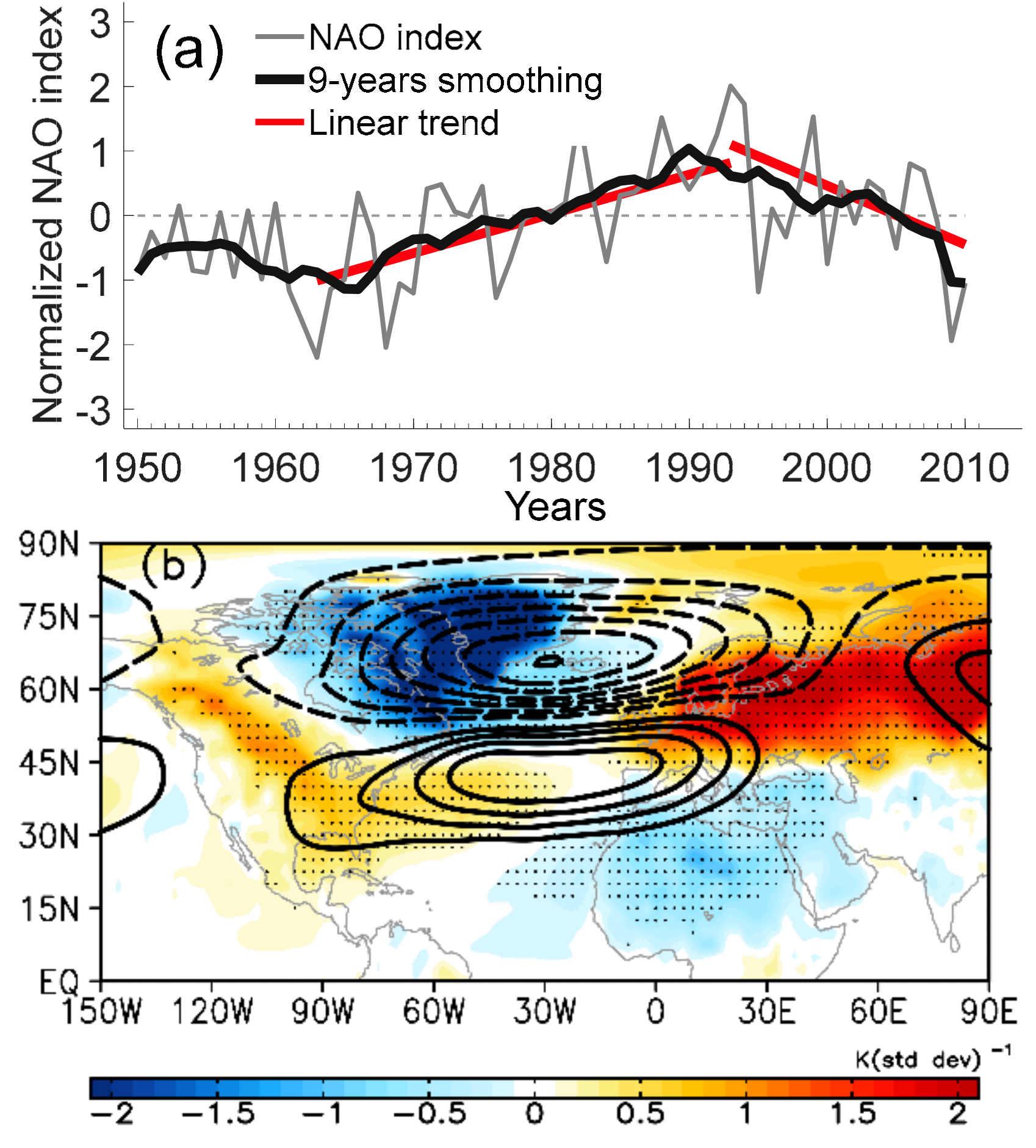
The winter mean NAO index from 1950 to 2010 is shown in Figure 1a. It is clear to see that the NAO index exhibits significant decadal and mutidecadal variabilities. The NAO index is mainly negative during 1950–1980, and then turns positive during 1980–2010. Specifically, the winter NAO index undergoes a linear upward trend from 1963 to 1993, followed by a downward trend from 1994 to 2010, as indicated in Figure 1a, which was investigated by Luo et al. [24,25,26,27]. The regression pattern of the NAO is shown in Figure 1b, from which we can see the classical meridional dipole mode. The dipole centers are basically north–south symmetrical (at the same longitude) and the north center has a greater amplitude and range than the south center [3,9]. The SAT anomaly on the continent exhibits a quadrupole mode, with a significant positive (negative) SAT over Europe and America (Canada and north Africa). The two SAT anomaly centers over the north have a stronger amplitude than the SAT anomaly centers over the south. This is due to the physical process by which the NAO circulation affects the SAT, which was investigated by Yao and Luo [4]. Since this study’s focus is on the tilt of the NAO dipole mode, further analysis in this respect is not be applied.
3.2. Composites of NAO+ and NAO− Events
As shown in Figure 1b, the dipole mode is the most important feature of the NAO pattern. However, for each NAO case and different phases, the dipole mode has its own characteristics, including strength, position [28,29], and many other aspects such as zonal shifting [30,31]. The NAO events are further divided into NAO+ and NAO− events to reveal their dipole characteristics.
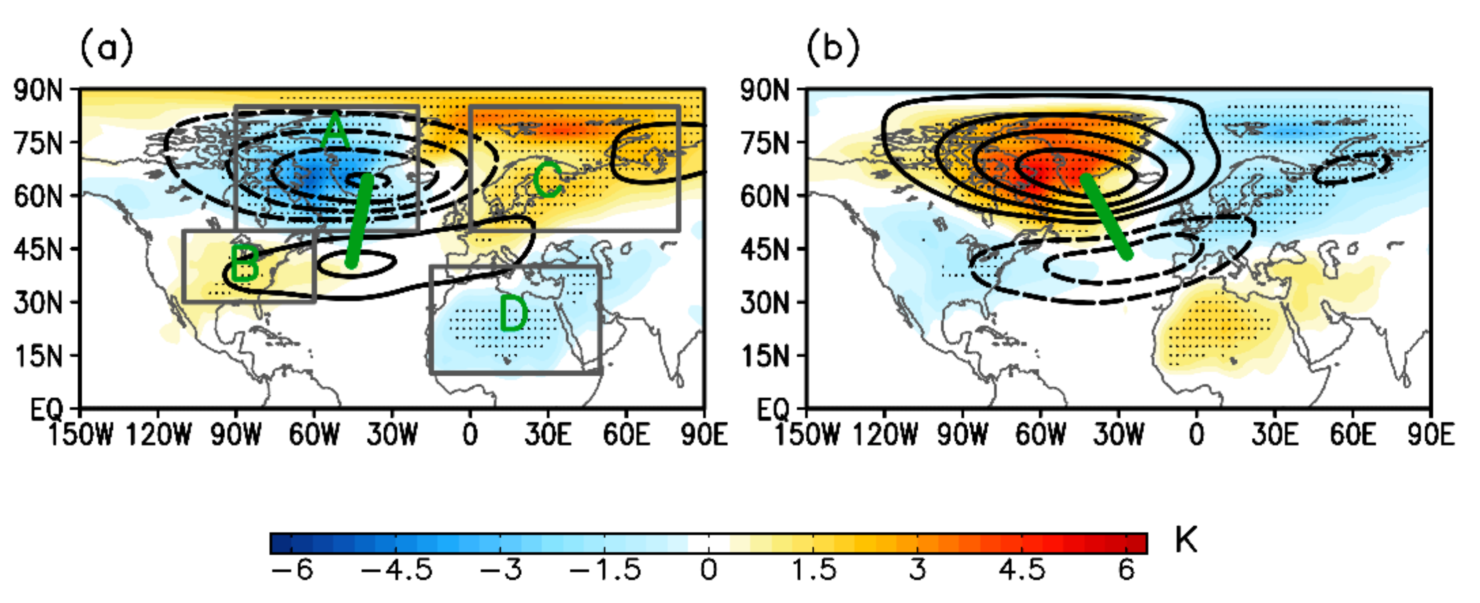
Based on the winter daily NAO index and the definition of NAO events, 152 NAO+ events and 161 NAO− events are identified. The composites of geopotential height and SAT anomaly from lag −5 to lag 5 days of the NAO events during the winter period from 1950 to 2011 are shown in Figure 2. It can be seen that the NAO+ event exhibits a north-over-south dipole mode with a negative center at higher latitude and a positive center at lower latitude. In addition, it is found that the straight line (green line in Figure 2a) between the negative and positive anomaly centers has a slight tilt angle along the northeast–southwest (NE–SW) direction. Meanwhile, for NAO− (Figure 2b), it is clear that a positive-over-negative dipole mode exists in the North Atlantic region. Interestingly, the straight line (green line in Figure 2b) between the dipole centers exhibits a visible northwest–southeast (NW–SE) tilting, which is opposite to the tilting direction of the NAO+ dipole shown in Figure 2a. Figure 2 also displays the composite SAT anomalies for NAO+ and NAO− events, from which it is clear that the SAT pattern for both NAO+ and NAO− features a spatial asymmetric quadrupole mode, but with opposite phases. In Figure 2a, a spatial asymmetric dipole SAT anomaly pattern is apparent over the North American continent, with a wide and strong negative anomaly center over Greenland and a slight positive anomaly center over the eastern United States. Moreover, a positive SAT anomaly center exists over north Europe and the Greenland Basin, and a negative SAT anomaly center exists over north Africa and the Middle East (Figure 2a). An opposite spatial asymmetric SAT quadrupole mode phase can be seen in Figure 2b.
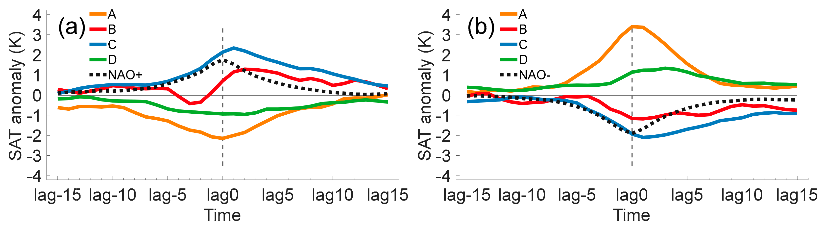
To further examine the regional variability of the SAT within the NAO life cycle, four sub-regions (A: 90°–20° W, 50°–85° N; B: 100°–60° W, 30°–50° N; C: 0°–80° E, 50°–85° N; D: 15° W–50° E, 10°–40° N) are defined based on the SAT quadrupole pattern, as shown in Figure 2 (grey boxes). Figure 3 shows the SAT series by averaging over the four sub-regions from lag −15 to lag 15 of the NAO+ (Figure 3a) and NAO− (Figure 3b) life cycles. The black dotted line represents the composite NAO index, and the orange, red, blue and green lines represent the SAT series for regions A, B, C and D, respectively. It is clear that the SAT in region C (blue line) exhibits a 1 day lag with the NAO index (Figure 2). The SAT in B and D lag the NAO index by about 2 to 3 days. The variation of SAT in A is basically synchronous with the NAO index. Moreover, it is found that the SAT anomaly in region A (orange lines) has the largest contrast in amplitude with other regions during the NAO life cycle. This may be due to the fact that region A is located almost at the center of the NAO northern anomaly center, where the SAT is most affected by the NAO circulation. That is why the SAT in region A is almost in sync with the NAO’s development. The remaining regions (B, C and D) are located south and downstream of the north center of the NAO dipole, and the SAT changes in these regions will lag behind the NAO’s development due to the delayed evolution of physical processes such as the temperature advection. Actually, the lead-lag relationship between SAT and NAO is also affected by the choice of metrics and regions.
The tilt of the dipole mode for large-scale circulation is an important structural feature according to previous studies that have focused on blocking dipole patterns [5,19]. Due to the different physical mechanisms involved, the tilt of the dipole pattern can be a significant determinant of the pathway of cold air invasion, leading to the occurrence of extreme weather [5]. This serves as a motivation to further examine the tilt pattern of the NAO dipole and its different climate impacts. As shown in Figure 2, the mean dipole pattern of NAO+ (NAO−) events exhibits an NE–SW (NW–SE) tilting direction. This may indicate that most of the NAO+ (NAO−) cases possibly exhibit NE–SW (NW–SE) tilting. However, the frequency and variability of the NAO dipole tilt is still not clear. In the following, by examining each NAO case, the tilting direction and further SAT impacts are examined.
3.3. Definition of NAO Dipole Tilt
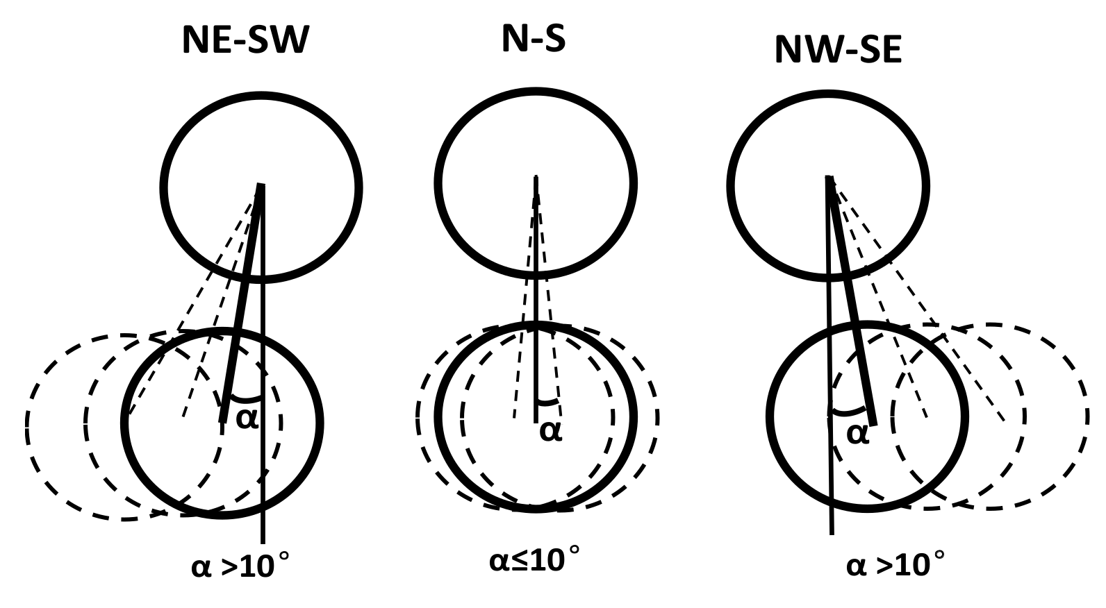
In this part, the tilting feature of the NAO dipole pattern for each single event is identified by examining the daily geopotential height anomaly. Figure 4 is a schematic diagram of the NAO dipole and its tilting characteristic. By using the geopotential height anomaly pattern during the strong stage (lag 0 or average of lag −1 to 1) of each NAO event, the tilt angle (α, as indicated in Figure 4) of the line between positive and negative geopotential height anomaly centers is examined. For the NAO dipole centers, if the intersection angle (α) between the core line (point-to-point line between dipole centers, as indicated in Figure 4) and meridian direction is not 0°, the NAO dipole will exhibit a tilting feature. In order to pick out notable tilted NAO events, here, an NAO dipole pattern is called a tilted NAO dipole pattern if the intersection angle (α) between the core line and meridian direction exceeds 10° (as shown in Figure 4); otherwise, it has no tilting characteristic. According to this definition, the tilting types of the NAO dipole can be divided into NE–SW tilting, north–south symmetric (N–S, not tilted), and NW–SE tilting, as indicated in Figure 4.
3.4. Frequency and Variability of the NAO Dipole Tilting
Based upon the tilting definition, by examining the geopotential height anomaly of the NAO peak stage (mean of lag −1 to lag 1) for each NAO event, all NAO events are classified into N–S, NE–SW and NW–SE tilting types. Table 1 shows the event numbers of different tilting types for NAO+ and NAO− events. It is found that, in total, there are 152 NAO+ and 161 NAO− events during the winters of 1950–2011. For the 152 NAO+ events, 23 (15.1%) are N–S type, 64 (42.1%) are NE–SW tilting type, and 65 (42.8%) are NW–SE tilting type. Of the 161 NAO− events, 28 (17.4%) are N–S type, 41 (25.5%) are NE–SW tilting type, and 92 (57.1%) are NW–SE tilting type. Note that identification using the lag 0 of each NAO event was also applied, and the results were qualitatively consistent. However, the average of peak stage (lag −1 to lag 1) days is more representative and stable than that of lag 0 day. In order to avoid the noise of mesoscale systems and obtain more stable NAO tilt cases, the NAO tilt events divided according to the peak stage (mean of lag −1 to lag 1) are used in the following analysis. It is clear that N–S is the type with the lowest proportion of all NAO events, which may suggest that the asymmetric pattern is the dominant feature for both NAO+ and NAO− events. For NAO+ events, the number of NE–SW and NW–SE tilting events is almost the same, possibly leading to slight NE–SW tilting or no tilting for the mean NAO+ dipole, as shown in Figure 2a. The number of NW–SE tilting NAO− events (92) accounts for 57.1% of all NAO− events, which is more than twice the number of NE–SW tilting NAO− events (41, accounting for 25%). Therefore, the mean pattern of the NAO− dipole mode exhibits a visible NW–SE tilting characteristic, as shown in Figure 2b.
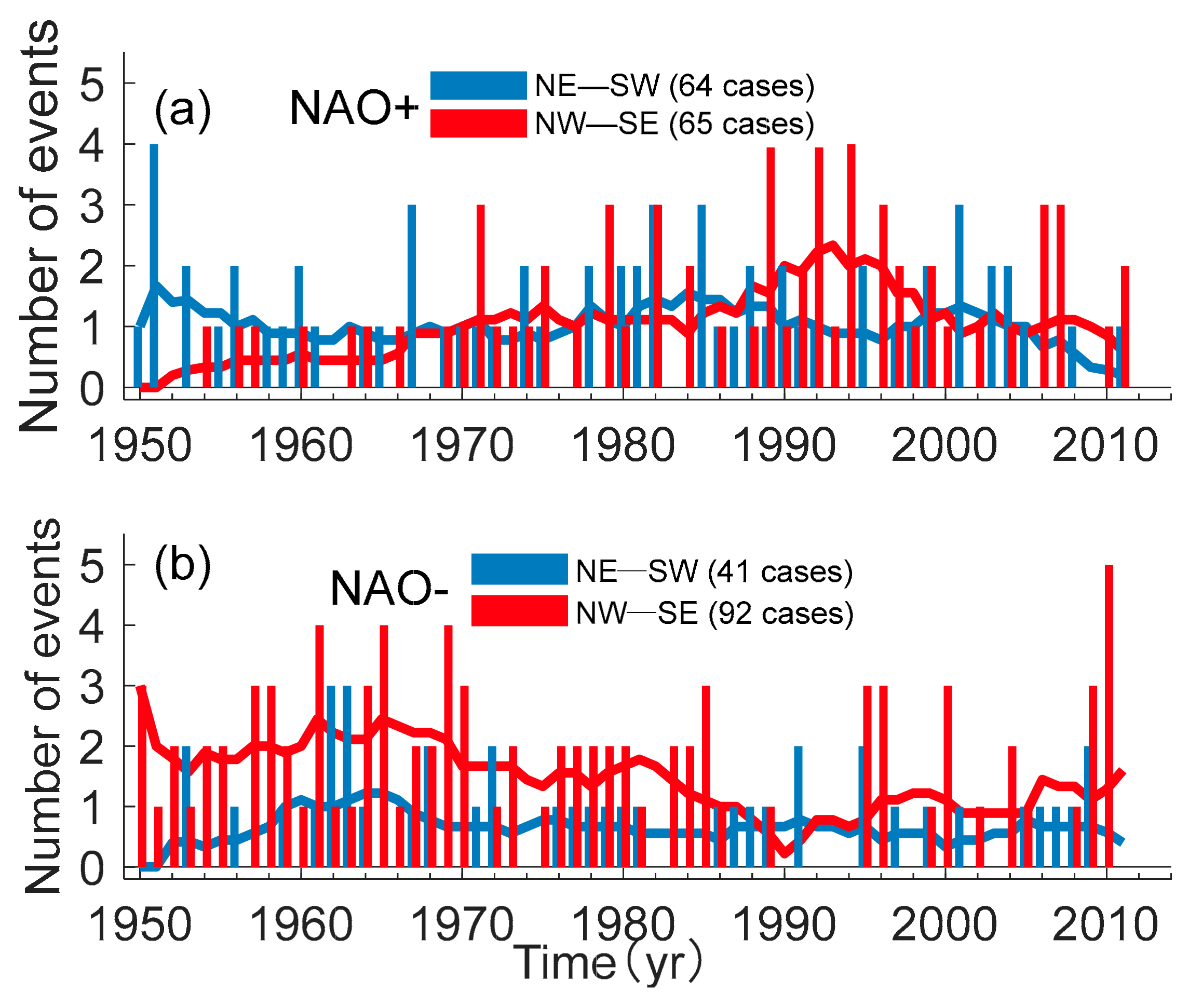
Figure 5 displays the time series of the frequency of the NAO+ and NAO− tilting events from 1950 to 2010. It is found that, for NAO+ events, the frequency of NW–SE tilting events exhibits a decadal variability, from a lower frequency during 1950–1970 to a dominant frequency during 1970–2010 (Figure 5a). In addition, the decadal variation of NW–SE tilting NAO− events changes from a dominant frequency during 1950–1987 to a lower frequency during 1988–2010, as can be seen in Figure 5b. However, regarding the frequency of NE–SW tilting NAO events, the decadal variation is not significant. It is further found that the variation of the number of NW–SE NAO+ (NAO−) events has a significant positive (negative) correlation coefficient of 0.51 (−0.65) with the NAO index, both of which are significant above the 99% confidence level. This indicates that the variations of NW–SE NAO events usually have a trend that is closely related with the NAO index. Given that the frequency of N–S NAO events is small and the asymmetric feature is weak, the time series of its frequency is not shown in Figure 5. Also, the analysis of N–S NAO events is not shown in the following section. To further examine the characteristics of different NAO tilting types, the results from composite analysis are presented in the following section.
4. Composite Analysis of NAO Tilting Classification
4.1. Structure and SAT Impacts of Different NAO Tilts
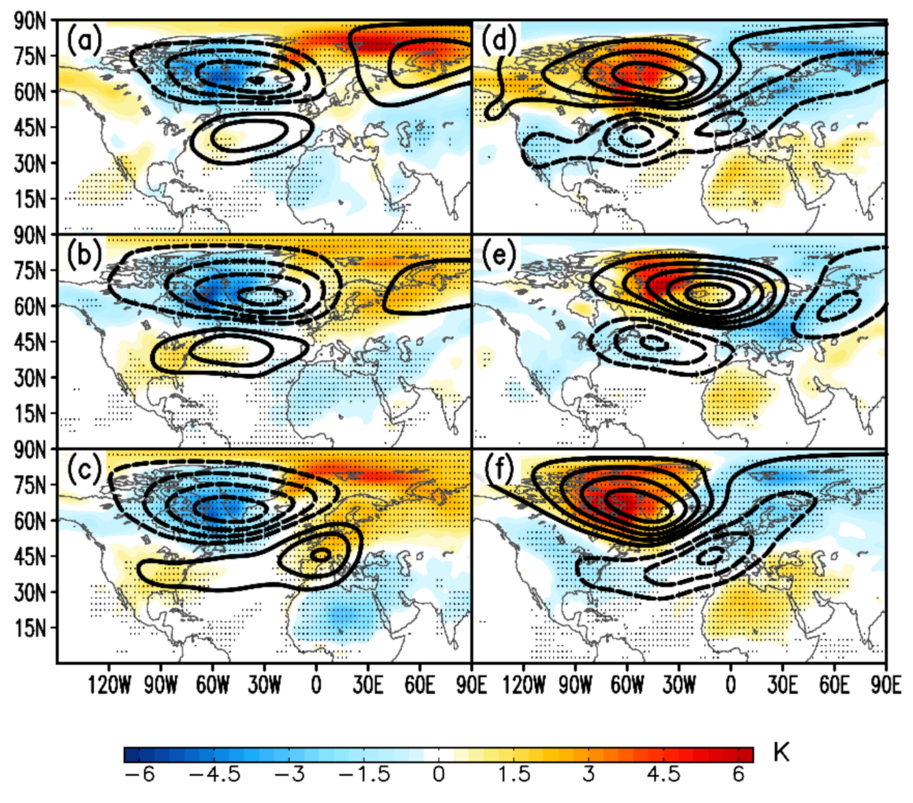
Based on the classification of the types of NAO dipole tilting, composites of geopotential height and SAT anomalies are shown in Figure 6. It is found that the quadrupole mode of the geopotential height and SAT anomalies can be seen in all types of NAO tilting events. However, for different tilting NAO events, they are different from each other in position, strength, extent, and many other aspects. Figure 6a–c show the composites for N–S, NE–SW and NW–SE tilting NAO+ events (Figure 6d–f show the composites for N–S, NE–SW and NW–SE tilting NAO−), respectively. It can be seen that the core line direction between the dipole centers of N–S NAO events is almost parallel to the meridian direction in Figure 6a,d. As shown in Figure 6b,e, NE–SW (Figure 6c,f NW–SE) tilting NAO+ and NAO− events both exhibit a notable NE–SW (NW–SE) dipole tilting structure. For NW–SE tilting NAO+ events (Figure 6c), the negative SAT anomaly over north Africa and the Middle East is much stronger and wider than for NE–SW and N–S NAO+ events. Meanwhile, the NW–SE tilting NAO+ events (Figure 6c) can lead to a marked positive SAT anomaly over western and northern Europe compared with N–S and NE–SW tilting NAO+ events. It is clear that the positive geopotential height anomaly center for NW–SE NAO+ events (Figure 6c) is located more eastward (even extending to west Europe) than for N–S NAO+ and NE–SW NAO+ events. Moreover, the negative geopotential height anomaly center for NW–SE NAO+ events (Figure 6c) is located more westward than for N–S NAO+ (Figure 6a) and NE–SW NAO+ events (Figure 6b). Thus, the dipole anomaly centers for NW–SE NAO+ events inevitably exhibit a NE–SW tilting structure. The tilting structure for NW–SE NAO− events in Figure 6f is similar to that of NW–SE NAO+ events in Figure 6c. The SAT pattern for NW–SE NAO− events is almost equivalent to the pattern for NW–SE NAO+ events multiplied by −1. The negative SAT anomalies are located over north Europe for N–S and NW–SE NAO− events, while the negative SAT anomaly is mainly located over south Europe for NE–SW NAO− events. The results suggest that the SAT anomaly pattern for NAO events is dominated by the dipole structure of the NAO, especially the tilt direction. Notable asymmetric spatial patterns of geopotential height and SAT can be observed during the NAO life cycle.
4.2. Temporal Variations of SAT Anomaly during the NAO Life Cycle
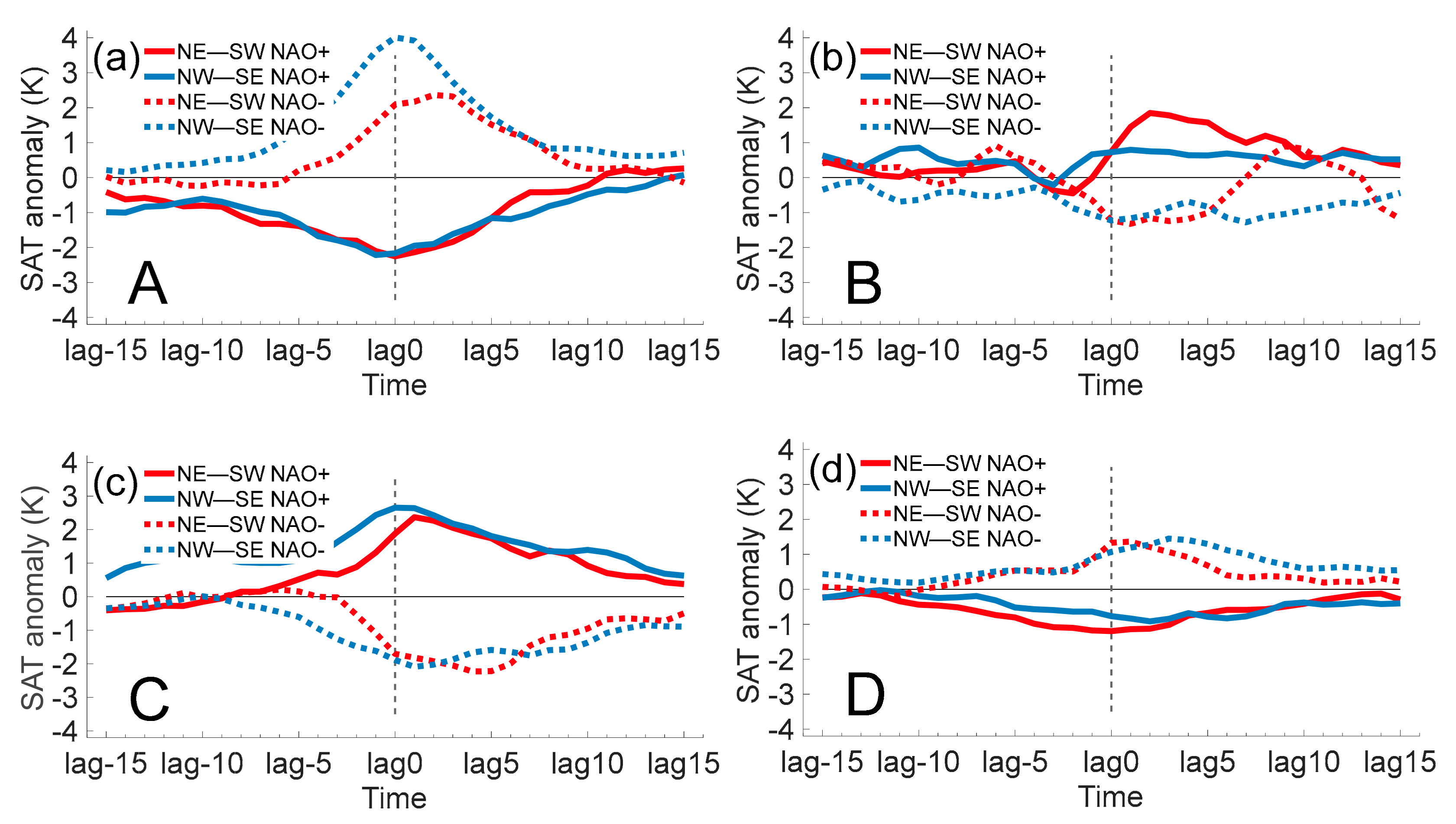
Figure 7 shows the time series of the regional mean SAT anomaly for regions A–D during the life cycle of different tilting NAO events. It can be seen in Figure 7a that the SAT anomalies for region A exhibit a significantly synchronous change with NE–SW NAO+, NW–SE NAO+, and NW–SE NAO− evolution. However, for NE–SW NAO− events, the SAT anomaly in region A exhibits a slight lag relationship (1 day) with the NAO’s evolution. This might be due to the NE–SW tilting of the NAO dipole, as shown in Figure 6e. The north center (anticyclone) of the dipole mode is located more northeasterly and farther away form region A compared with the other tilting NAO events. Thus, the SAT changes for region A may lag behind the evolution of NE–SW NAO− due to the delayed transfer of the warm advection. Although NE–SW NAO+ exhibits a northeast–southwest tilting pattern (Figure 6b), its tilt angle is far smaller than that of the NE–SW NAO− dipole (Figure 6e). Therefore, the SAT anomaly change in region A shows no lag relationship with NE–SW NAO+ events (Figure 7a). The positive SAT anomaly in region A for NW–SE NAO− events has a stronger amplitude compared with other events (Figure 7a). This might be due to the distribution of the positive SAT anomaly, as shown in Figure 6f, which covers most of region A’s extent and thus has a higher averaging value. Region A is the area that is closest to the NAO’s north center and most affected by the NAO’s circulation. This can also be seen in Figure 6 in that the SAT anomaly in region A has the maximum amplitude compared with other regions.
For region B, the change in SAT anomalies during the NAO’s life cycle can be seen in Figure 7b. It is clear that the change in the SAT anomalies lags the NAO’s evolution by about 1–2 days. Also, the SAT anomalies in region B have weaker amplitudes compared with region A. For regions C and D (Figure 7c,d), the SAT anomalies also exhibit a significant lag relationship (about 1–4 days) with the NAO’s evolution. Because regions C and D are located downstream of the NAO dipole mode, the associated SAT change will lag behind the NAO’s circulation due to the delayed change in related temperature advection.
5. Physical Mechanism of the NAO Dipole Tilt
5.1. Zonal Jet Distributions of Different NAO+ Tilting Events
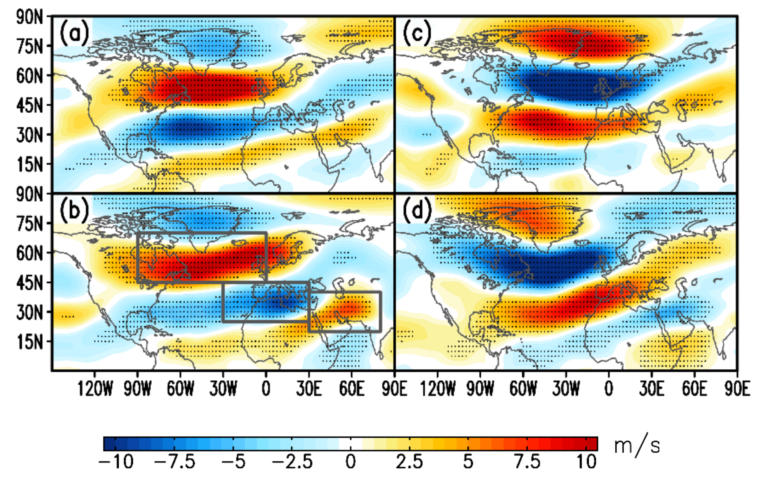
Regarding the tilt of the NAO dipole, some studies have proposed that the self-advection by stronger or weaker winds may lead to a SW–NE tilt of the NAO+ [30], while the tropics anomaly may force an NW–SE tilt NAO pattern remotely through a poleward Rossby wave [32]. According to previous studies [2,3,4,17], the zonal jet has a key dynamic impact on the evolution of the NAO’s circulation, such as its position, strength, and life cycle. In order to examine the physical mechanism behind the NAO dipole tilt, the 300 hPa zonal wind anomaly during the life cycles of different tilting NAO events is shown in Figure 8. For NAO+ events (Figure 8a,b), it can be seen that the 300 hPa zonal wind anomaly centers exhibit a negative–positive–negative–positive distribution from north to south. Also, a positive–negative–positive–negative distribution from north to south can be seen for NAO− events in Figure 8c,d, which shows opposite distribution phases to the NAO+ events. However, for different tilting NAO events, there are significant differences in the distribution of zonal wind anomalies. For NE–SW NAO+ and NW–SE NAO+ events, although quadrupole centers from north to south can be observed in Figure 8a,b, there are clear differences in location and strength. Specifically, for NW–SE NAO+ events (Figure 8b), the negative anomaly center over 30°N is located at about 0°–30°E. Meanwhile, the negative anomaly center over 30°N for NE–SW NAO+ events is located near 60°W (Figure 8a), which is more westward than for NW–SE NAO+ events. Moreover, the southernmost positive anomaly center for NW–SE NAO+ events is located more eastward than that for NE–SW NAO+ events. Also, the maximum core of this positive anomaly center is more northeast (the easternmost black frame in Figure 8b) than in Figure 8a.
For NAO− events, as shown in Figure 8c,d, significant differences can also be found. The quadrupole centers from north to south exhibit a NE–SW tilt distribution (Figure 8c), which is consistent with the NE–SW NAO dipole tilt direction. Meanwhile, as shown in Figure 8d, the quadrupole centers from north to south exhibit a NW–SE tilt characteristic, which does match with the tilt direction of the NW–SE NAO dipole. This can be explained by the positive feedback mechanism between the NAO’s circulation and the zonal wind jet. According to previous studies [4,33,34], complicated feedback and a self-mechanism exists between the NAO and westerly wind. Generally, the variation of the zonal wind over the North Atlantic region and the evolution of the NAO’s circulation are accompanying processes. The development of NAO events will adjust the zonal wind distribution due to the evolution of the anticyclone and cyclone of the NAO dipole mode. Specifically, NAO+ will lead to a strengthening of the zonal jet axis at middle and high latitudes, showing a strong jet, while NAO− will divide the jet stream into two branches—one at high latitudes and the other at middle and low latitudes. This can also be clearly seen in Figure 8. However, the NAO’s circulation is not the only factor affecting the zonal wind distribution. The SST distribution over the Atlantic, topographic action, and other factors can also make important contributions to the zonal wind variations. If the zonal wind anomaly distribution exhibits a tilting characteristic before the beginning of the NAO, then it can be regarded as an initial disturbance field before the NAO’s development. Also, the evolution of the NAO’s circulation will further affect the zonal wind distribution, which can be referred to as a feedback mechanism.
Therefore, due to the drive of the zonal jet distribution, the NAO dipole mode may show different tilt characteristics. The zonal wind spatial distribution over the North Atlantic prior to the NAO’s onset can significantly affect the NAO’s evolution, especially the NAO dipole mode. However, the zonal wind spatial distribution over the North Atlantic is significantly affected by the Atlantic SST distribution. Thus, in the following section, we examine the associated SST distribution.
5.2. SST Anomaly Pattern of Different NAO+ Tilting Events
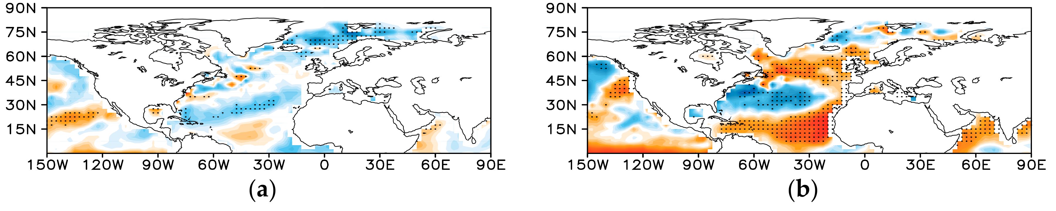
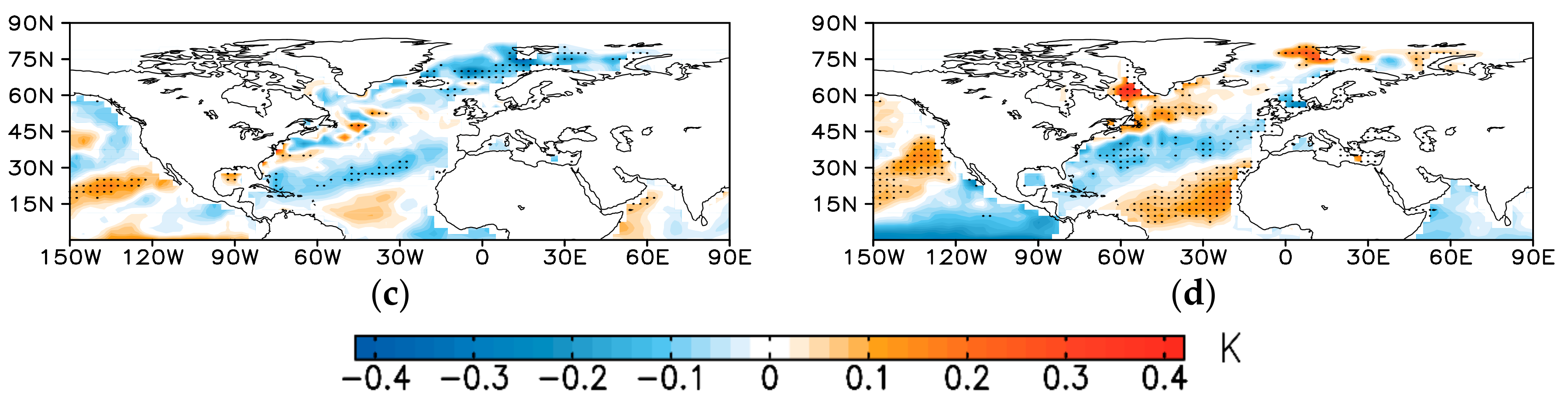
Figure 9 shows the composite SST anomalies over the Atlantic from lag −5 to lag 5 of the NAO life cycle. For NAO+ events (Figure 9a,b), the SST anomalies over the Atlantic exhibit a positive tripole mode, with one positive anomaly center at midlatitudes and two negative anomaly centers at low and mid–high latitudes. This is the classic positive tripole SST mode that is associated with NAO+ events, as indicated in previous studies [10,35,36]. However, the SST tripole patterns between NE–SW (Figure 9a) and NW–SE (Figure 9b) NAO+ events have some differences. The midlatitude positive SST anomaly center for NE–SW NAO+ events presents a distinct distribution and is located northward compared with NW–SE NAO+ events. Also, another positive anomaly center can be observed at low latitudes south of 15°N. In addition, a significant positive center can be seen at high latitudes (near the Greenland and Barents seas) for NW–SE NAO+ events. Although this positive center is not in the range of the tripole SST mode, the difference in the SST anomaly distribution between NE–SW and NW–SE NAO+ events is significant. The clear positive SST anomaly center over the polar region might be related to the positive SAT anomaly center that is associated with the NW–SE NAO+ events, as shown in Figure 6c. However, the causality between SAT and SST is a nonlinear and complicated process beyond the scope of the present study. For NE–SW (Figure 9c) and NW–SE (Figure 9d) NAO− events, an opposite SST tripole pattern compared with NAO+ events can be seen over the Atlantic. Notably, the SST anomaly for NE–SW NAO− events in Figure 9c is greater than for the other three NAO types, possibly because of the lack of balance in the numbers of events, with NE–SW NAO− events having the smallest number (41) of cases. The amplitude of the anomalies is lower on average compared with the other three types of events. Moreover, the northern positive center of the SST tripole in Figure 9c is located more eastward than that of Figure 9d; plus, the central negative center of the SST tripole in Figure 9d has a wider and more eastward distribution compared with that in Figure 9c. This means that the SST tripole anomalies for NE–SW NAO+ events are more inclined to exhibit an NE–SW tilt, which might stimulate the initiation and growth of the NAO pattern to exhibit an NE–SW tilt. The change in the SST tripole anomaly is a slow process relative to atmospheric circulation such as the NAO. Therefore, to some extent, the SST tripole anomaly provides a background state for the development of the NAO dipole tilting direction. Also, the development of the NAO and its tilting characteristic might feedback positively to the maintenance of the SST tripole anomaly. The SST tripole anomaly affects the NAO dipole tilt mainly through regulating the distribution of the zonal wind, from the low-level wind to the upper jet axis. Many other studies have also examined the relationship between NAO and SST using model experiments, which suggested that the SST forcing has important impact on the NAO development [37,38]. Furthermore, the SST patterns in the Pacific also show differences, which may affect the upstream zonal wind that influences the downstream atmospheric circulation, which needs to be examined in the future. The interaction between the zonal jet and the NAO’s circulation is a complicated self-maintaining mechanism and nonlinear process, as indicated in Yao and Luo [4], which is not discussed in detail in this study.
5.3. Decadal Variability and Its Possible Causal Relationships
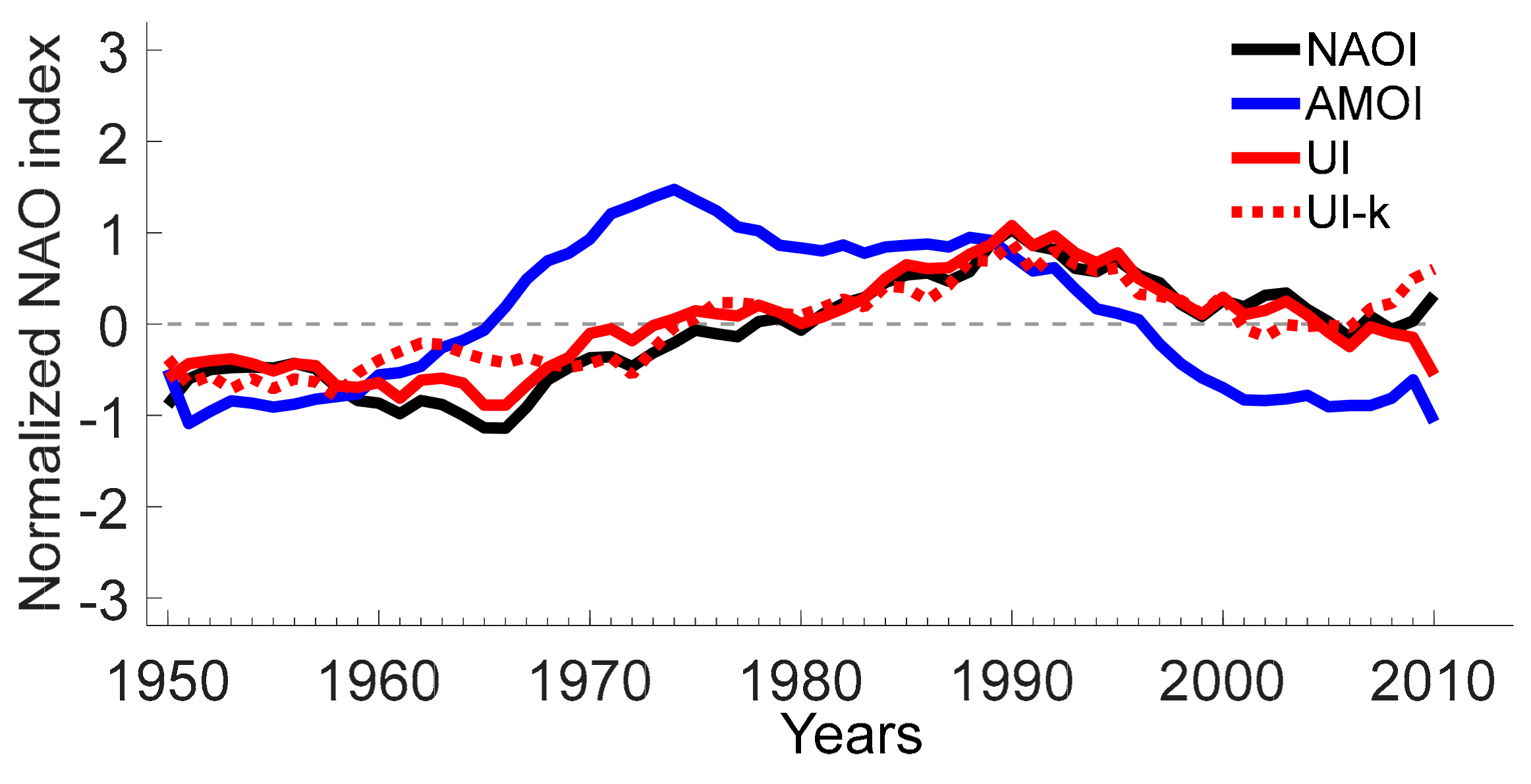
As indicated in Figure 5, the time series of the number of NAO events exhibit significant interdecadal and decadal variability, especially for NAO+ NW–SE and NAO− NW–SE events. In order to examine the possible physical processes that cause the interdecadal and decadal variation, Figure 10 shows the AMO and self-constructed U index series. It is found that the AMO index (multiplied by −1.0) exhibits clear interdecadal and decadal variations, showing a peak phase from 1970 to 1990. Meanwhile, to reflect the dynamic characteristic of the NAO index, a zonal wind index is constructed based on the dipole pattern of the NAO and wind distribution in Figure 8. As shown in Figure 8b, the three boxes (boxes A, B and C from high to low latitudes) represent three zonal wind anomaly centers, and a wind index based is constructed based on the regional mean wind anomaly of the three regions (, and ) according to the formula . The index () can represent the change of the westerly jet and the degree of difference of the westerly at different latitudes. Specifically, the three regions are arranged from west to east and from high to low latitudes. Therefore, UI can also represent the tilting characteristics of the maximum westerly core at different latitudes to some extent. Moreover, UIK is defined, which is an extended index based on . Before calculating , all the NAO individual life cycle days are removed from the zonal wind anomaly fields . Then, is calculated using the formula , based on the zonal wind anomaly fields without NAO days. Thus, represents an index that removes the effect of the NAO positive feedback to the zonal wind and may represent the basic field that affects the regional circulation, such as the NAO.
It can be seen from Figure 10 that the NAO exhibits a clear multidecadal variability from a dominant negative-phase epoch (1950–1980) to a dominant positive-phase epoch (1980–2010). The physical mechanism of the NAO interdecadal, decadal and multidecadal variability has been examined previously with both observational data and theoretical tools [24,39]. In addition, it is found that exhibits very similar interdecadal and decadal variations to those of the NAO index. The background zonal wind with NAO days removed () also exhibits interdecadal and decadal variability that is highly relevant to that of the NAO index. Although represents the zonal wind with the NAO days removed, the interdecadal and decadal variabilities of and are very consistent, with a high correlation coefficient of 0.64 (0.83 for nine-point smoothed indices, as seen in Table 2). This indicates that the regional background zonal wind has an important impact on the local atmospheric circulation, such as the NAO. Furthermore, the development of the local atmospheric circulation has an important feedback mechanism to the basic stream (background zonal wind), which includes a complicated nonlinear and self-maintaining mechanism between the NAO and basic stream, as proposed by Luo et al. [34]. The atmospheric basic zonal wind in the Atlantic region can be affected by the variation of the Atlantic SST, according to previous studies [10,36]. Therefore, if a dominant SST signal can be found, it will be meaningful for understanding the change in the tilt of the NAO dipole, especially in terms of the decadal or multidecadal variability. As the most dominant oceanic signal in the Atlantic, the AMO has a significant influence on local weather and atmospheric circulation. It can be found that the AMO may have a lead–lag relationship with the NAO index, as shown in Figure 10. Through calculation, it can be seen that the AMO might lead the NAO index by approximately 15 years and has a correlation coefficient of 0.47 (0.84 for smoothed indices). However, the lead–lag relationship between NAO and SST has been examined in many previous studies [40,41], indicating that the NAO leads the SST. Actually, for different time scales, the lead–lag relationship between NAO and SST may be different. The atmospheric variation is a fast process, while the ocean change is a slow process. The change of the NAO may affect (lead) the regional SST on a synoptic time scale while the SST background (slow change) may also affect the NAO variation on a synoptic time scale [42,43].
Table 2 shows the correlation coefficients between associated indices. It is found that the AMO index (multiplied by −1.0) has a significant 15-year lead relationship with the NAO index, and , especially on interdecadal and decadal scales. All the correlation coefficients between nine-point smoothed indices are above the 99% confidence level based on a hypothesis test. This suggests that the AMO can significantly affect and then regulate and the NAO circulation with a 15-year lead. It is further found that , and the AMO index also have a good correlation relationship with the frequencies of NW–SE NAO+ and NW–SE NAO−. Although the numbers of NW–SE NAO+ and NE–SW NAO+ events are almost the same (64 and 65 cases), the frequency of NW–SE NAO+ has a clearer positive correlation relationship with the NAO index, and . This means that the NAO index may well indicate the interdecadal and decadal variability of NW–SE NAO+ events. Moreover, the AMO index may indicate the interdecadal and decadal variability of NW–SE NAO+ events 15 years ahead. NW–SE NAO+, as an important NAO type, has a significant effect on Eurasian extreme cold weather, as revealed in previous studies [5,19]. The results presented here may have some reference value for the statistical prediction of Eurasian extreme cold weather on interdecadal and decadal time scales. In addition, the frequency of NW–SE NAO− also has a significant relationship with the AMO index, NAO index, and . This is of great significance in terms of understanding the change in the frequency of different NAO tilting types.
6. Conclusions and Discussion
In this study, according to the climatic characteristics of the NAO dipole mode and the tilt characteristics of the dipole centers, NAO events are divided into NE–SW, N–S and NW–SE tilting NAO events. The spatial asymmetric quadrupole structure of the SAT anomaly can be observed during the NAO life cycle. Due to the different distributions of the dipole centers between different NAO tilt events, the SAT quadrupole structure also shows significant differences. In addition, the temporal evolution of the quadrupole SAT anomaly also shows lead–lag differences between difference NAO tilt events. This is mainly due to the difference in the cold and warm advection paths caused by the different positions of cyclones and anticyclones. It is suggested that the tilt of the NAO dipole is crucial for the SAT change locally. The frequency of NW–SE NAO+ (−) events exhibits similar (opposite) interdecadal and decadal change to the NAO index and . This means that the basic zonal flow can be seen as a background that affects the regional atmospheric circulation, subsequently causing the NAO dipole to tilt, and generating a specific tilt feature under a specific westerly background configuration. It is found that , which is defined based on three key regional mean zonal winds, can be seen as an index that reflects the frequency of NW–SE NAO+ (or −) events.
The physical mechanism by which the SST drives the change in NAO tilting by affecting the basic zonal flow is also examined. It is indicated that, for NE–SW, N–S and NW–SE tilting NAO events, the Atlantic SST anomaly patterns show clear differences during the NAO life cycle (synoptic time scale).
It is found that the AMO is a very clear signal that leads the change of by about 15 years on interdecadal and decadal time scales. The SST anomaly pattern during the NAO life cycle is a slower process of change compared with that of the NAO itself, even though the SST is affected by feedback from the NAO’s circulation. Excluding the interaction between the SST and NAO, there must be a stronger signal providing the long-term climatic basic state of the SST change. As the most dominant SST anomaly pattern in the North Atlantic, the AMO can provide a strong background SST state on interdecadal to multidecadal time scales. It can be seen that the negative SST anomaly center in Figure 9b at around 60°N is at a very similar location to the strongest AMO positive anomaly center. This means that the AMO may provide a stable, long-term climatic basic SST state on decadal or even multidecadal time scales in this region. Through long-term and slow physical processes, such as oceanic circulation, the “memory” of ocean heat capacity, etc., it changes the distribution of SST, subsequently affecting the change in the atmospheric basic zonal flow and then leading to the change in the NAO dipole tilt on synoptic time scales. This could perhaps be referred to as a “temporal downscaling” process. In the present study, the AMO index is multiplied by −1.0, and thus the negative AMO index may promote (inhibit) the appearance of NW–SE tilting NAO+ (−) events. It is worth mentioning that this promotion or inhibition effect operates about 15 years ahead of the change in the NAO. Therefore, to some extent, this study might be helpful for the long-term prediction of the NAO dipole tilt pattern, as well as some disastrous weather processes, such as blizzards, that might be caused by NW–SE tilting NAO+ events.
Funding
This research was funded by the Chinese Academy of Sciences Strategic Priority Research Program (Grant XDA19070403) and the National Natural Science Foundation of China (Grants 41975068 and 41790473).
Conflicts of Interest
The authors declare no conflict of interest.
References
- Hurrell, J.W. Decadal Trends in the North-Atlantic Oscillation—Regional Temperatures and Precipitation. Science 1995, 269, 676–679. [Google Scholar] [CrossRef] [PubMed] [Green Version]
- Feldstein, S.B. The dynamics of NAO teleconnection pattern growth and decay. Q. J. R. Meteorol. Soc. 2003, 129, 901–924. [Google Scholar] [CrossRef]
- Benedict, J.J.; Lee, S.; Feldstein, S.B. Synoptic view of the North Atlantic Oscillation. J. Atmos. Sci. 2004, 61, 121–144. [Google Scholar] [CrossRef] [Green Version]
- Yao, Y.; Luo, D.H. An Asymmetric Spatiotemporal Connection between the Euro-Atlantic Blocking within the NAO Life Cycle and European Climates. Adv. Atmos. Sci. 2018, 35, 796–812. [Google Scholar] [CrossRef]
- Yao, Y.; Luo, D.H.; Dai, A.G.; Feldstein, S.B. The Positive North Atlantic Oscillation with Downstream Blocking and Middle East Snowstorms: Impacts of the North Atlantic Jet. J. Clim. 2016, 29, 1853–1876. [Google Scholar] [CrossRef]
- Iles, C.; Hegerl, G. Role of the North Atlantic Oscillation in decadal temperature trends. Environ. Res. Lett. 2017, 12, 114010. [Google Scholar] [CrossRef]
- Moore, G.W.K.; Renfrew, I.A. Cold European winters: Interplay between the NAO and the East Atlantic mode. Atmos. Sci. Lett. 2012, 13, 1–8. [Google Scholar] [CrossRef]
- Yu, B.; Lupo, A.R. Large-Scale Atmospheric Circulation Variability and Its Climate Impacts. Atmosphere 2019, 10, 329. [Google Scholar] [CrossRef] [Green Version]
- Luo, D.H. A barotropic envelope Rossby soliton model for block-eddy interaction. Part I: Effect of topography. J. Atmos. Sci. 2005, 62, 5–21. [Google Scholar] [CrossRef]
- Peng, S.L.; Robinson, W.A.; Li, S.L. Mechanisms for the NAO responses to the North Atlantic SST tripole. J. Clim. 2003, 16, 1987–2004. [Google Scholar] [CrossRef]
- Lupo, A.R.; Jensen, A.D.; Mokhov, I.I.; Timazhev, A.V.; Eichler, T.; Efe, B. Changes in Global Blocking Character in Recent Decades. Atmosphere 2019, 10, 92. [Google Scholar] [CrossRef] [Green Version]
- Yao, Y.; Luo, D.H. Do European Blocking Events Precede North Atlantic Oscillation Events? Adv. Atmos. Sci. 2015, 32, 1106–1118. [Google Scholar] [CrossRef]
- Cohen, J.; Barlow, M. The NAO, the AO, and global warming: How closely related? J. Clim. 2005, 18, 4498–4513. [Google Scholar] [CrossRef]
- Feldstein, S.B. The recent trend and variance increase of the annular mode. J. Clim. 2002, 15, 88–94. [Google Scholar] [CrossRef]
- Hanna, E.; Cropper, T.E.; Hall, R.J.; Cappelen, J. Greenland Blocking Index 1851–2015: A regional climate change signal. Int. J. Climatol. 2016, 36, 4847–4861. [Google Scholar] [CrossRef] [Green Version]
- Ulbrich, U.; Christoph, M. A shift of the NAO and increasing storm track activity over Europe due to anthropogenic greenhouse gas forcing. Clim. Dyn. 1999, 15, 551–559. [Google Scholar] [CrossRef]
- Luo, D.H.; Diao, Y.N.; Feldstein, S.B. The Variability of the Atlantic Storm Track and the North Atlantic Oscillation: A Link between Intraseasonal and Interannual Variability. J. Atmos. Sci. 2011, 68, 577–601. [Google Scholar] [CrossRef]
- Luo, D.H.; Chen, Y.N.; Dai, A.G.; Mu, M.; Zhang, R.H.; Simmonds, I. Winter Eurasian cooling linked with the Atlantic Multidecadal Oscillation. Environ. Res. Lett. 2017, 12, 125002. [Google Scholar] [CrossRef] [Green Version]
- Luo, D.H.; Yao, Y.; Dai, A.G.; Feldstein, S.B. The Positive North Atlantic Oscillation with Downstream Blocking and Middle East Snowstorms: The Large-Scale Environment. J. Clim. 2015, 28, 6398–6418. [Google Scholar] [CrossRef]
- Knight, J.R.; Maidens, A.; Watson, P.A.G.; Andrews, M.; Belcher, S.; Brunet, G.; Fereday, D.; Folland, C.K.; Scaife, A.A.; Slingo, J. Global meteorological influences on the record UK rainfall of winter 2013–2014. Environ. Res. Lett. 2017, 12, 074001. [Google Scholar] [CrossRef] [Green Version]
- Kalnay, E.; Kanamitsu, M.; Kistler, R.; Collins, W.; Deaven, D.; Gandin, L.; Iredell, M.; Saha, S.; White, G.; Woollen, J.; et al. The NCEP/NCAR 40-year reanalysis project. Bull. Am. Meteorol. Soc. 1996, 77, 437–471. [Google Scholar] [CrossRef] [Green Version]
- Barnston, A.G.; Livezey, R.E. Classification, Seasonality and Persistence of Low-Frequency Atmospheric Circulation Patterns. Mon. Weather. Rev. 1987, 115, 1083–1126. [Google Scholar] [CrossRef]
- Enfield, D.B.; Mestas-Nunez, A.M.; Trimble, P.J. The Atlantic multidecadal oscillation and its relation to rainfall and river flows in the continental US. Geophys. Res. Lett. 2001, 28, 2077–2080. [Google Scholar] [CrossRef] [Green Version]
- Luo, D.H.; Yao, Y.; Dai, A.G. Decadal Relationship between European Blocking and the North Atlantic Oscillation during 1978–2011. Part I: Atlantic Conditions. J. Atmos. Sci. 2015, 72, 1152–1173. [Google Scholar] [CrossRef]
- Bracegirdle, T.J.; Lu, H.; Eade, R.; Woollings, T. Do CMIP5 Models Reproduce Observed Low-Frequency North Atlantic Jet Variability? Geophys. Res. Lett. 2018, 45, 7204–7212. [Google Scholar] [CrossRef]
- Scaife, A.A.; Knight, J.R.; Vallis, G.K.; Folland, C.K. A stratospheric influence on the winter NAO and North Atlantic surface climate. Geophys. Res. Lett. 2005, 32, L18715. [Google Scholar] [CrossRef] [Green Version]
- Shindell, D.T.; Schmidt, G.A.; Miller, R.L.; Rind, D. Northern Hemisphere winter climate response to greenhouse gas, ozone, solar, and volcanic forcing. J. Geophys. Res. Atmos. 2001, 106, 7193–7210. [Google Scholar] [CrossRef] [Green Version]
- Luo, D.H.; Yao, Y.; Feldstein, S.B. Regime Transition of the North Atlantic Oscillation and the Extreme Cold Event over Europe in January–February 2012. Mon. Weather. Rev. 2014, 142, 4735–4757. [Google Scholar] [CrossRef] [Green Version]
- Yao, Y.; Luo, D.H. Relationship between zonal position of the North Atlantic Oscillation and Euro-Atlantic blocking events and its possible effect on the weather over Europe. Sci. China Earth Sci. 2014, 57, 2628–2636. [Google Scholar] [CrossRef]
- Peterson, K.A.; Lu, J.; Greatbatch, R.J. Evidence of nonlinear dynamics in the eastward shift of the NAO. Geophys. Res. Lett. 2003, 30, 1030. [Google Scholar] [CrossRef]
- Zuo, J.Q.; Ren, H.L.; Li, W.J.; Wang, L. Interdecadal Variations in the Relationship between the Winter North Atlantic Oscillation and Temperature in South-Central China. J. Clim. 2016, 29, 7477–7493. [Google Scholar] [CrossRef]
- Scaife, A.A.; Comer, R.E.; Dunstone, N.J.; Knight, J.R.; Smith, D.M.; MacLachlan, C.; Martin, N.; Peterson, K.A.; Rowlands, D.; Carroll, E.B.; et al. Tropical rainfall, Rossby waves and regional winter climate predictions. Q. J. R. Meteorol. Soc. 2017, 143, 1–11. [Google Scholar] [CrossRef]
- Luo, D.H.; Gong, T.T.; Lupo, A.R. Dynamics of eddy-driven low-frequency dipole modes. Part II: Free mode characteristics of NAO and diagnostic study. J. Atmos. Sci. 2007, 64, 29–51. [Google Scholar] [CrossRef] [Green Version]
- Luo, D.H.; Lupo, A.R.; Wan, H. Dynamics of eddy-driven low-frequency dipole modes. Part I: A simple model of North Atlantic oscillations. J. Atmos. Sci. 2007, 64, 3–28. [Google Scholar] [CrossRef]
- Frankignoul, C.; Kestenare, E. Observed Atlantic SST anomaly impact on the NAO: An update. J. Clim. 2005, 18, 4089–4094. [Google Scholar] [CrossRef]
- Pan, L.L. Observed positive feedback between the NAO and the North Atlantic SSTA tripole. Geophys. Res. Lett. 2005, 32, L06707. [Google Scholar] [CrossRef]
- Maidens, A.; Arribas, A.; Scaife, A.A.; MacLachlan, C.; Peterson, D.; Knight, J. The Influence of Surface Forcings on Prediction of the North Atlantic Oscillation Regime of Winter 2010/11. Mon. Weather Rev. 2013, 141, 3801–3813. [Google Scholar] [CrossRef]
- Nie, Y.; Ren, H.L.; Zhang, Y. The Role of Extratropical Air-Sea Interaction in the Autumn Subseasonal Variability of the North Atlantic Oscillation. J. Clim. 2019, 32, 7697–7712. [Google Scholar] [CrossRef]
- Luo, D.H.; Yao, Y.; Dai, A.G. Decadal Relationship between European Blocking and the North Atlantic Oscillation during 1978–2011. Part II: A Theoretical Model Study. J. Atmos. Sci. 2015, 72, 1174–1199. [Google Scholar] [CrossRef] [Green Version]
- Eden, C.; Willebrand, J. Mechanism of interannual to decadal variability of the North Atlantic circulation. J. Clim. 2001, 14, 2266–2280. [Google Scholar] [CrossRef]
- Li, J.P.; Wang, J.L.X.L. A modified zonal index and its physical sense. Geophys. Res. Lett. 2003, 30, 1632. [Google Scholar] [CrossRef]
- Hermanson, L.; Eade, R.; Robinson, N.H.; Dunstone, N.J.; Andrews, M.B.; Knight, J.R.; Scaife, A.A.; Smith, D.M. Forecast cooling of the Atlantic subpolar gyre and associated impacts. Geophys. Res. Lett. 2014, 41, 5167–5174. [Google Scholar] [CrossRef] [PubMed] [Green Version]
- Robson, J.; Sutton, R.; Smith, D. Predictable Climate Impacts of the Decadal Changes in the Ocean in the 1990s. J. Clim. 2013, 26, 6329–6339. [Google Scholar] [CrossRef]
Figure 1.
(a) Time series of the North Atlantic Oscillation (NAO) index in winter (NDJFM) from 1950 to 2010. The grey line represents the winter yearly NAO index, the thick black line is the 9-year smoothed index, and the red lines are the linear trends for 1963–1993 and 1993–2010. (b) Linear regression of DJF-mean 500-hPa height [contour interval = 10; units: gpm (std dev)−1] and surface air temperature (SAT) (color shading) anomaly fields projected onto the NAO index in (a), in which the dotted areas represent SAT values that are above the 99% confidence level based on a two-sided Student’s t-test.

Figure 2.
Composites of the 500 hPa geopotential height anomaly (contours with 30 gpm intervals) and SAT anomaly (°C, shaded) from lag −5 to lag 5 days for (a) NAO+ and (b) NAO− events identified by the winter (NDJFM) daily NAO index from 1950 to 2010. The dotted areas represent SAT values that are above the 99% confidence level based on a two-sided Student’s t-test. The contour interval is 30 gpm. The regions with black boxes are four sub-regions (A: 90°–20° W, 50°–85° N; B: 110°–60° W, 30°–50° N; C: 0°–80° E, 50°–85° N; D: 15° W–50° E, 10°–40° N).

Figure 3.
Regional mean of the composite SAT anomaly (°C, shaded) from lag −15 to lag 15 days for (a) NAO+ and (b) NAO− events in four sub-regions (A–D; see Figure 2). Lag 0 represents the peak day of the NAO life cycle.
Figure 3.
Regional mean of the composite SAT anomaly (°C, shaded) from lag −15 to lag 15 days for (a) NAO+ and (b) NAO− events in four sub-regions (A–D; see Figure 2). Lag 0 represents the peak day of the NAO life cycle.

Figure 4.
Schematic diagram of the NAO tilting dipole centers: NE–SW NAO (left); N–S NAO (middle); and NW–SE NAO (right). The critical angle (α) is 10°.
Figure 4.
Schematic diagram of the NAO tilting dipole centers: NE–SW NAO (left); N–S NAO (middle); and NW–SE NAO (right). The critical angle (α) is 10°.

Figure 5.
Event frequency series of (a) NAO+ and (b) NAO− events (light grey bars represent N–S NAO events; blue bars represent NE–SW events; red bars represent NW–SE NAO events).
Figure 5.
Event frequency series of (a) NAO+ and (b) NAO− events (light grey bars represent N–S NAO events; blue bars represent NE–SW events; red bars represent NW–SE NAO events).

Figure 6.
Composites of the geopotential height anomaly (contours with 30 gpm intervals) and SAT anomaly (°C, shaded) from lag −5 to lag 5 days for (a–c) NAO+ and (d–f) NAO− events: (a,d) N–S NAO; (b,e) NE–SW NAO; (c,f) NW–SE NAO. Dotted areas represent SAT values that are above the 99% confidence level based on a two-sided Student’s t-test. Lag 0 represents the peak day of the NAO life cycle.

Figure 7.
Regional mean of the composite SAT anomaly (°C, shaded) from lag −15 to lag 15 days for (a) region A, (b) region B, (c) region C, and (d) region D (see Figure 2), as indicated in the bottom-left of each panel. Lag 0 represents the peak day of the NAO life cycle. Solid (dashed) lines represent NAO+ (NAO−) events. Red (blue) lines represent SAT indices of NE–SW (NW–SE) events.

Figure 8.
Composites of the 300 hPa zonal wind anomaly (units: m/s; dotted areas are regions above the 99% confidence level for a two-sided Student’s t-test) from lag −5 to lag 5 days for (a) NE–SW NAO+, (b) NW–SE NAO+, (c) NE–SW NAO−, and (d) NW–SE NAO− events.
Figure 8.
Composites of the 300 hPa zonal wind anomaly (units: m/s; dotted areas are regions above the 99% confidence level for a two-sided Student’s t-test) from lag −5 to lag 5 days for (a) NE–SW NAO+, (b) NW–SE NAO+, (c) NE–SW NAO−, and (d) NW–SE NAO− events.

Figure 9.
Composites of the SST anomaly (units: K; dotted areas are regions above the 99% confidence level for a two-sided Student’s t-test) from lag −5 to lag 5 days for (a) NE–SW NAO+, (b) NW–SE NAO+, (c) NE–SW NAO−, and (d) NW–SE NAO− events.
Figure 9.
Composites of the SST anomaly (units: K; dotted areas are regions above the 99% confidence level for a two-sided Student’s t-test) from lag −5 to lag 5 days for (a) NE–SW NAO+, (b) NW–SE NAO+, (c) NE–SW NAO−, and (d) NW–SE NAO− events.


Figure 10.
Time series of the Atlantic Multidecadal Oscillation (AMO) index (blue line; multiplied by −1.0), NAO index (black line), U index (red solid line) and U index with NAO events removed (red dashed line) in winter from 1950 to 2010.
Figure 10.
Time series of the Atlantic Multidecadal Oscillation (AMO) index (blue line; multiplied by −1.0), NAO index (black line), U index (red solid line) and U index with NAO events removed (red dashed line) in winter from 1950 to 2010.


Table 1.
Numbers of NAO (North Atlantic Oscillation) events classified by tilting type in winter during 1950–2011.
Table 1.
Numbers of NAO (North Atlantic Oscillation) events classified by tilting type in winter during 1950–2011.
| Regime | NAO+ | NAO− | ||||
|---|---|---|---|---|---|---|
| Total Number | 152 | 161 | ||||
| Tilting Type | N–S | NE–SW | NW–SE | N–S | NE–SW | NW–SE |
| Number of Events | 23 | 64 | 65 | 28 | 41 | 92 |
Table 2.
Associated indices and their correlation coefficients, including the original correlation coefficient and the correlation coefficient after nine-point smoothing. Values to the right of the slash are the smoothed correlation coefficients. AMOI15 indicates that the correlation coefficient between the AMO (Atlantic Multidecadal Oscillation) index and the other indices is a 15-year lead relationship.
| Indices | NAOI | NW–SE NAO+ | NW–SE NAO− | ||
|---|---|---|---|---|---|
| NAOI | - | 0.89/0.95 | 0.49/0.86 | 0.51/0.81 | −0.65/−0.91 |
| - | - | 0.64/0.83 | 0.61/0.75 | −0.66/−0.79 | |
| - | - | - | 0.45/0.68 | −0.28/−0.67 | |
| AMOI15 | 0.47/0.84 | 0.30/0.65 | 0.20/0.60 | 0.26/0.56 | −0.32/−0.75 |
© 2019 by the author. Licensee MDPI, Basel, Switzerland. This article is an open access article distributed under the terms and conditions of the Creative Commons Attribution (CC BY) license (http://creativecommons.org/licenses/by/4.0/).
Share and Cite
MDPI and ACS Style
Yao, Y. Spatial Asymmetric Tilt of the NAO Dipole Mode and Its Variability. Atmosphere 2019, 10, 781. https://doi.org/10.3390/atmos10120781
AMA Style
Yao Y. Spatial Asymmetric Tilt of the NAO Dipole Mode and Its Variability. Atmosphere. 2019; 10(12):781. https://doi.org/10.3390/atmos10120781
Chicago/Turabian StyleYao, Yao. 2019. "Spatial Asymmetric Tilt of the NAO Dipole Mode and Its Variability" Atmosphere 10, no. 12: 781. https://doi.org/10.3390/atmos10120781
Note that from the first issue of 2016, this journal uses article numbers instead of page numbers. See further details here.