Author Contributions
Conceptualization, A.R. and F.R.; Data curation, F.R. and E.L.; Formal analysis, A.R., H.U.R.S., and E.L.; Funding acquisition, I.d.l.T.D.; Investigation, B.G.-Z.; Methodology, F.R. and H.U.R.S.; Project administration, I.d.l.T.D.; Resources, I.d.l.T.D.; Software, B.G.-Z. and E.L.; Supervision, H.U.R.S. and I.A.; Validation, I.A.; Visualization, B.G.-Z.; Writing—original draft, A.R. and F.R.; Writing—review and editing, I.A. All authors have read and agreed to the published version of the manuscript.
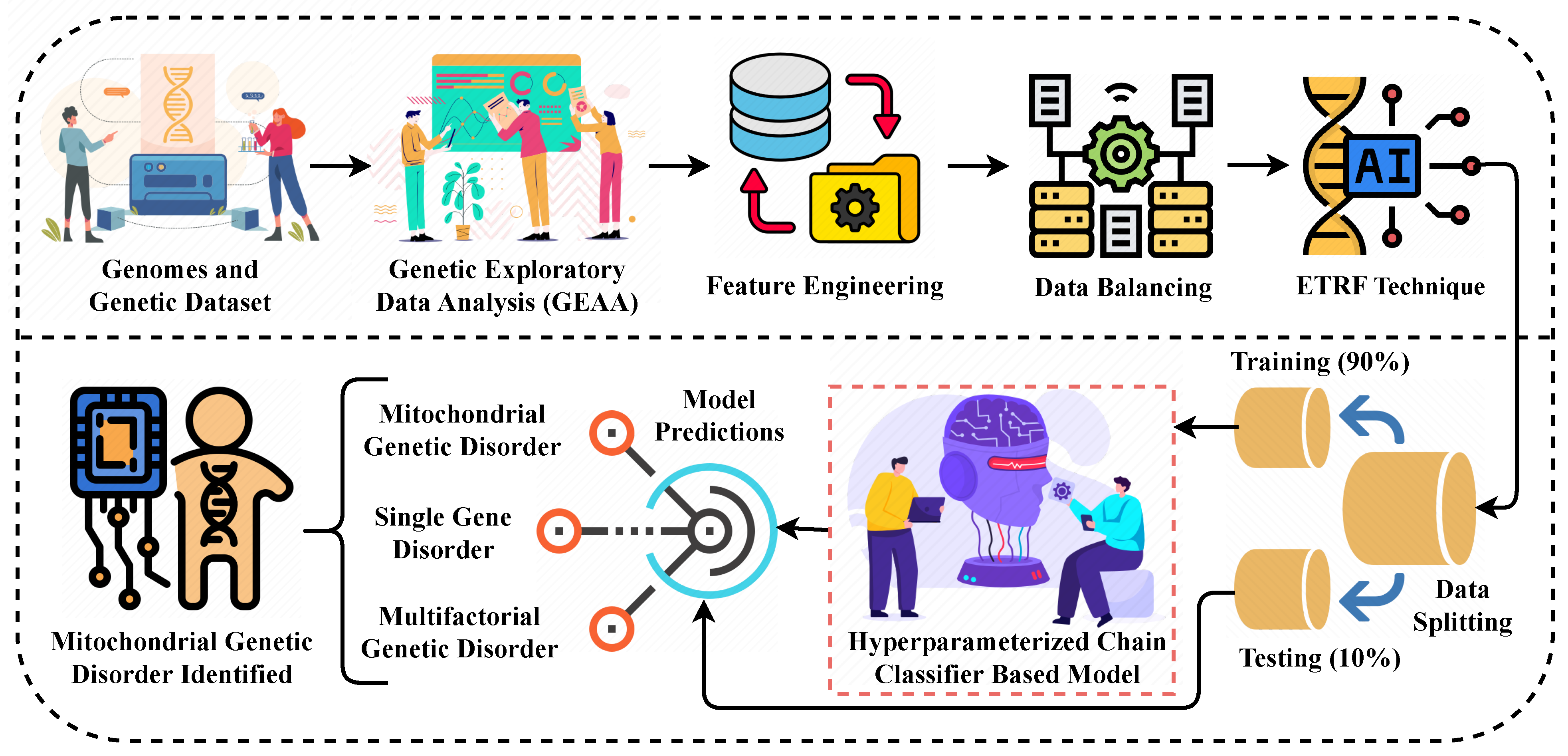
Figure 1.
The methodological analysis of our proposed research approach for predicting the genetic disorder and types of disorder.
Figure 1.
The methodological analysis of our proposed research approach for predicting the genetic disorder and types of disorder.
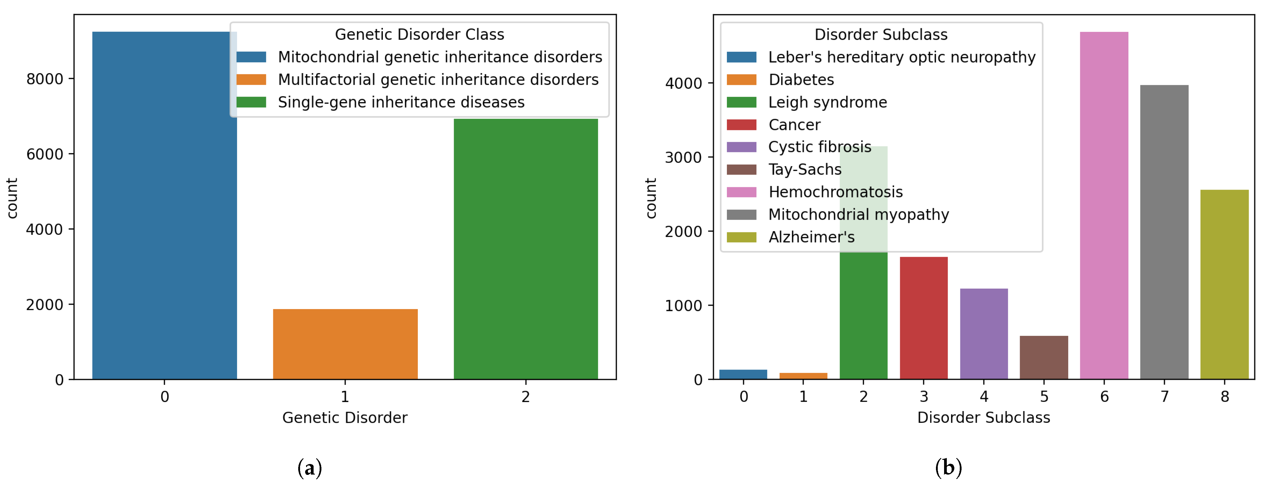
Figure 2.
Distributions of samples for different classes in the dataset, (a) genetic disorders’ main classes, and (b) genetic disorder subclasses.
Figure 2.
Distributions of samples for different classes in the dataset, (a) genetic disorders’ main classes, and (b) genetic disorder subclasses.
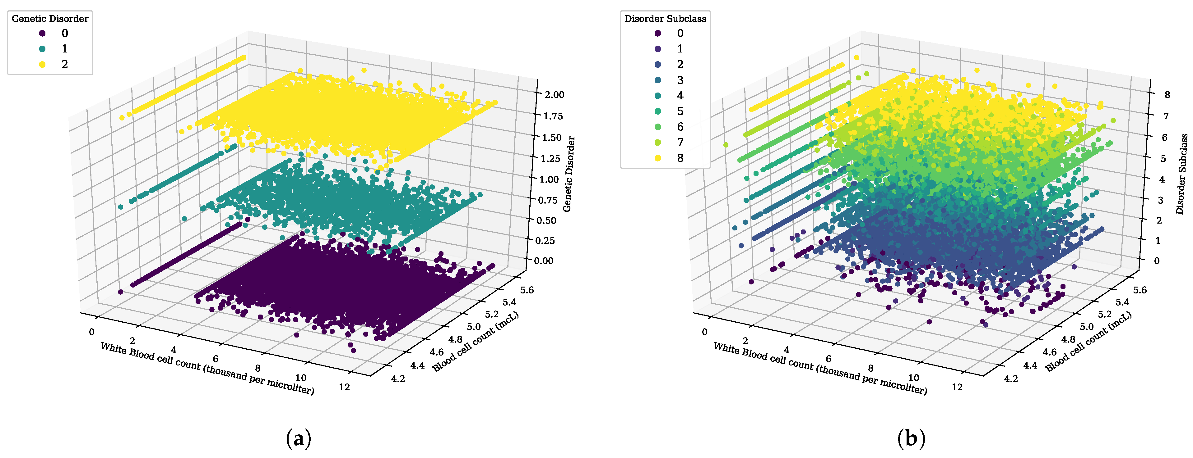
Figure 3.
The 3D scatter analysis for white blood cell count (thousand per microliter) and blood cell count (mcL), (a) genetic disorder category, and (b) genetic disorder sub-category.
Figure 3.
The 3D scatter analysis for white blood cell count (thousand per microliter) and blood cell count (mcL), (a) genetic disorder category, and (b) genetic disorder sub-category.
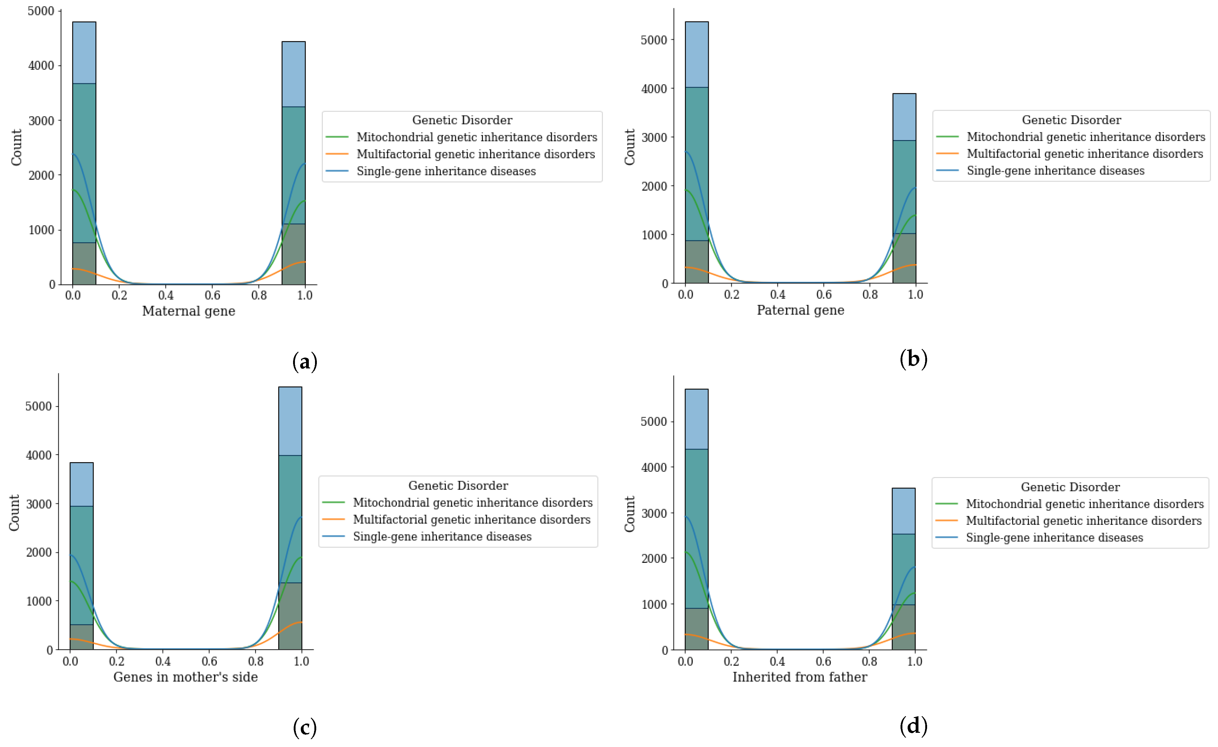
Figure 4.
Genomes data distribution by genetic disorder category, (a) maternal gene, (b) paternal gene, (c) genes from mother side, and (d) inherited from father.
Figure 4.
Genomes data distribution by genetic disorder category, (a) maternal gene, (b) paternal gene, (c) genes from mother side, and (d) inherited from father.
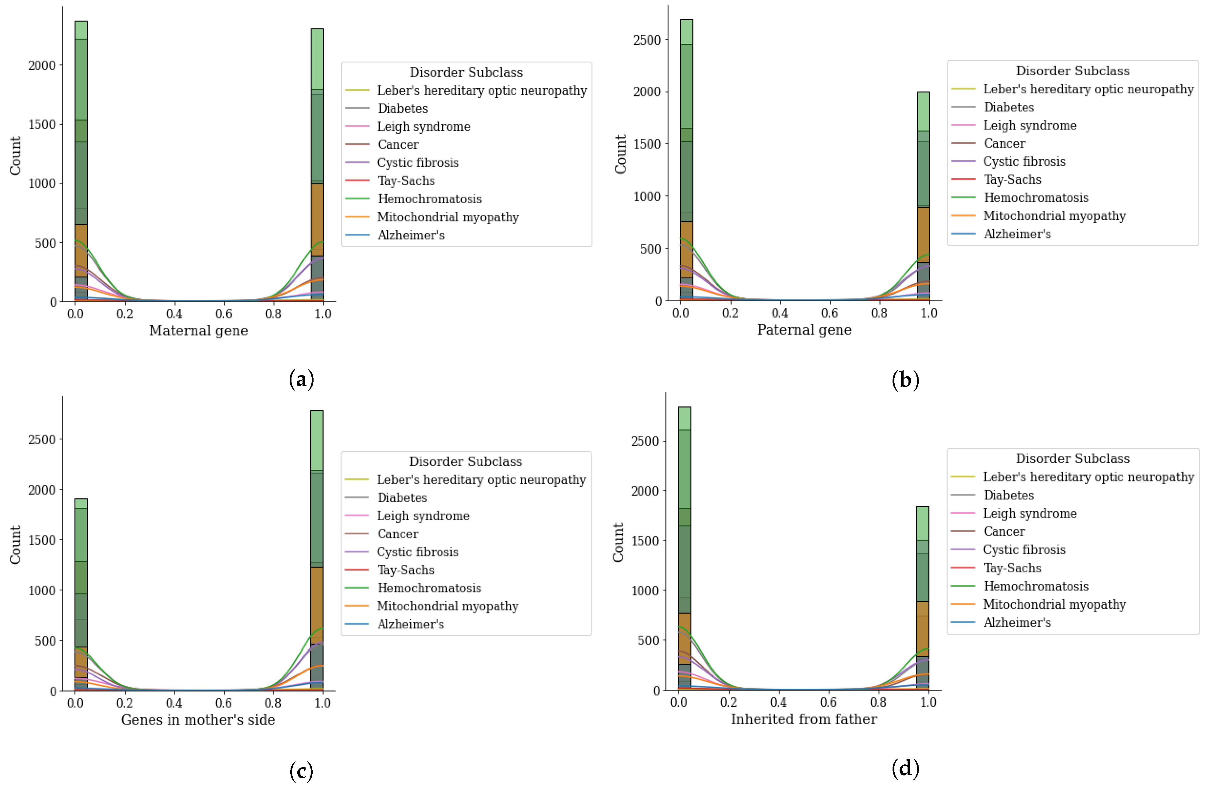
Figure 5.
Genomes data distribution by genetic disorder sub-category, (a) maternal gene, (b) paternal gene, (c) genes from mother side, and (d) inherited from father.
Figure 5.
Genomes data distribution by genetic disorder sub-category, (a) maternal gene, (b) paternal gene, (c) genes from mother side, and (d) inherited from father.
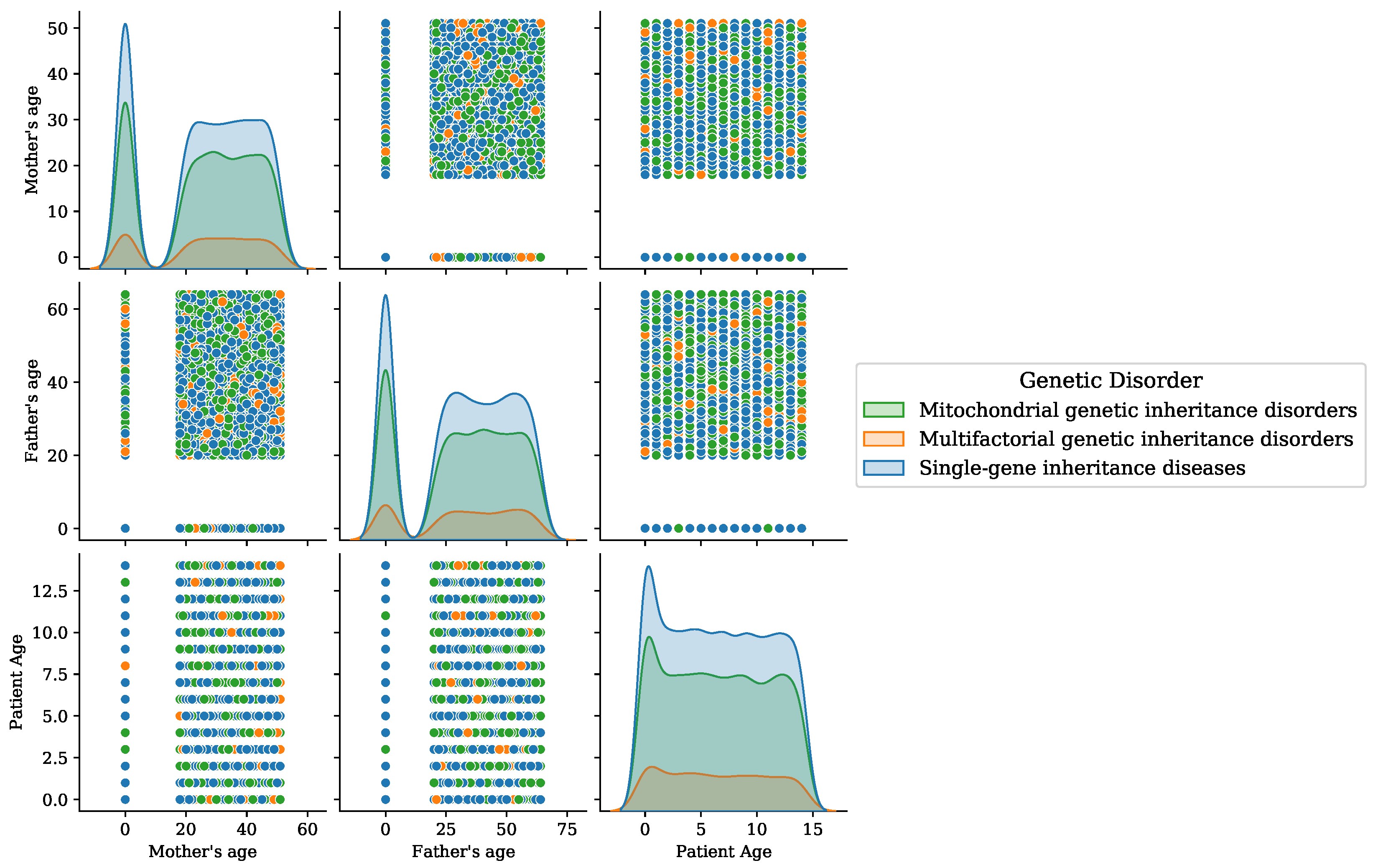
Figure 6.
Age analysis of patients for the disorder category.
Figure 6.
Age analysis of patients for the disorder category.
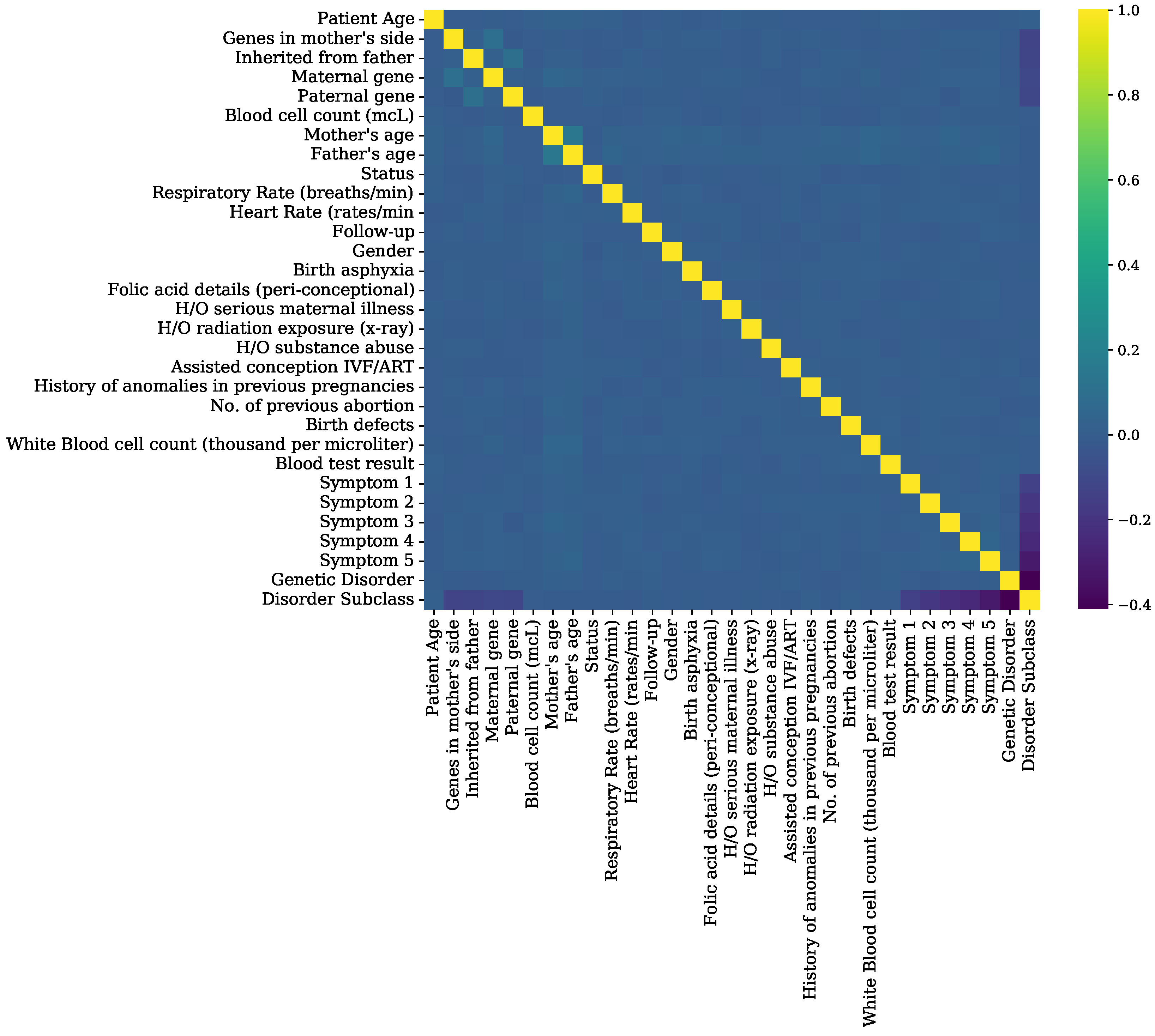
Figure 7.
Feature correlation analysis graphs of genomes data.
Figure 7.
Feature correlation analysis graphs of genomes data.
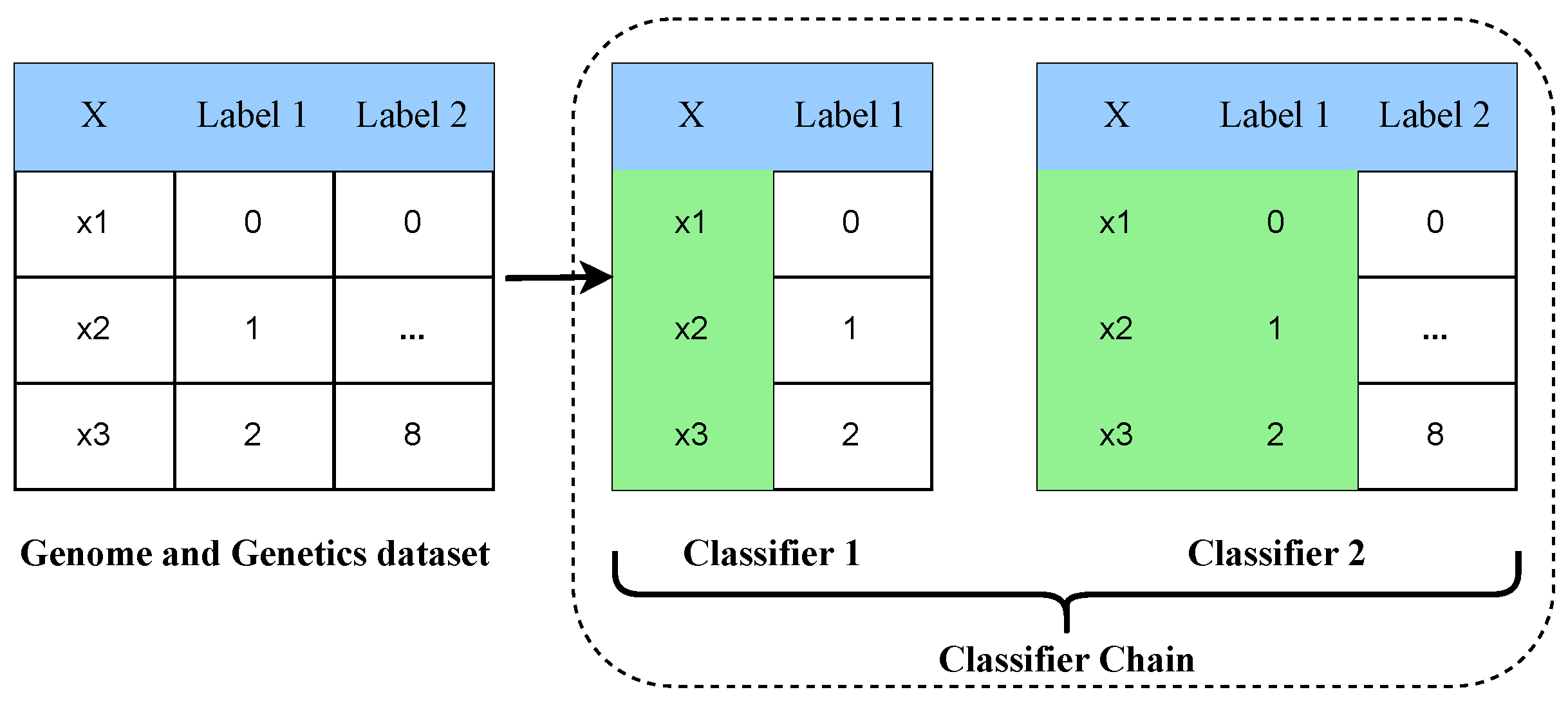
Figure 8.
The architectural analysis of the multi-label multi-class classifier chain approach.
Figure 8.
The architectural analysis of the multi-label multi-class classifier chain approach.
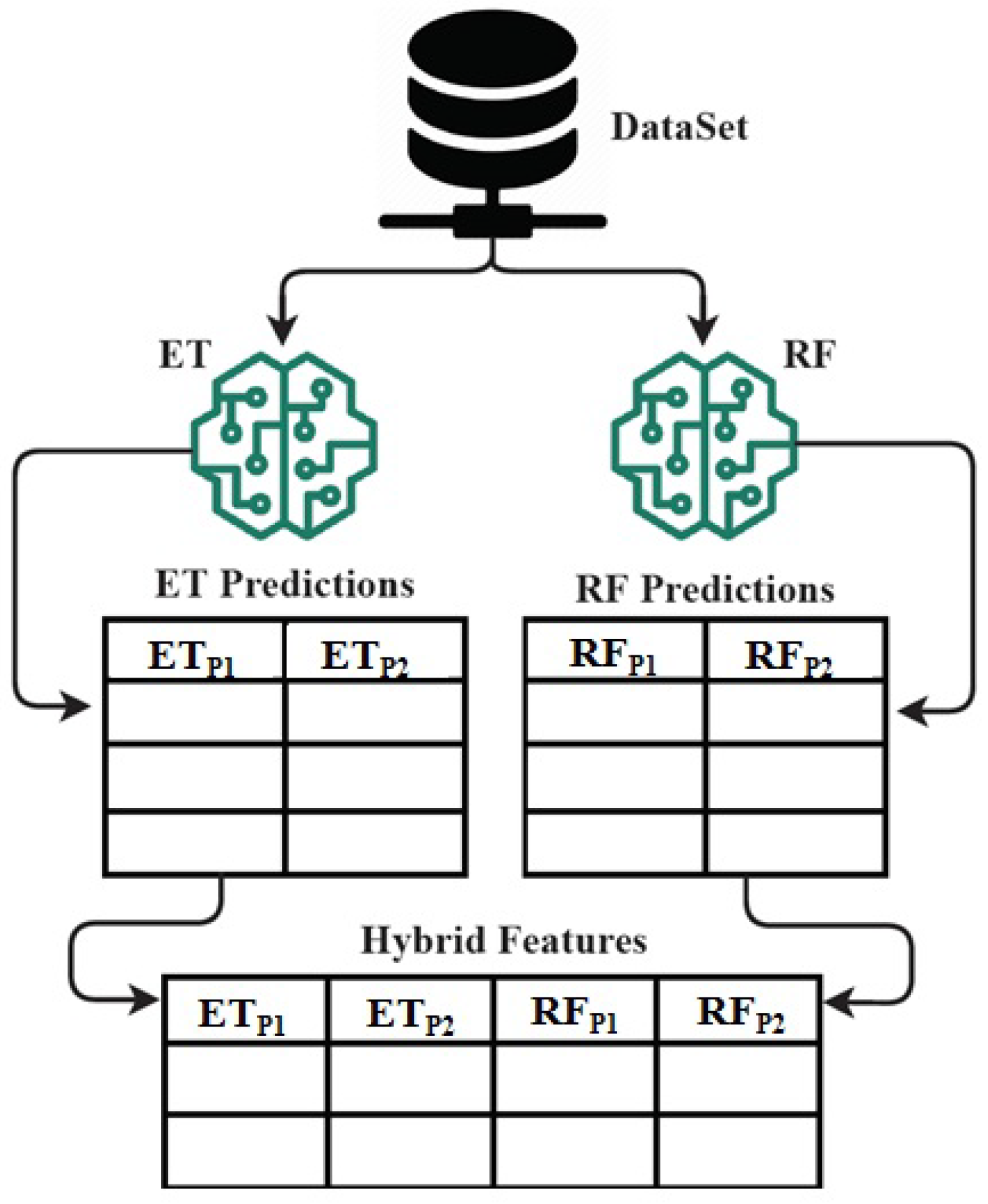
Figure 9.
The architecture analysis of proposed ETRF technique for hybrid feature set formation mechanism.
Figure 9.
The architecture analysis of proposed ETRF technique for hybrid feature set formation mechanism.
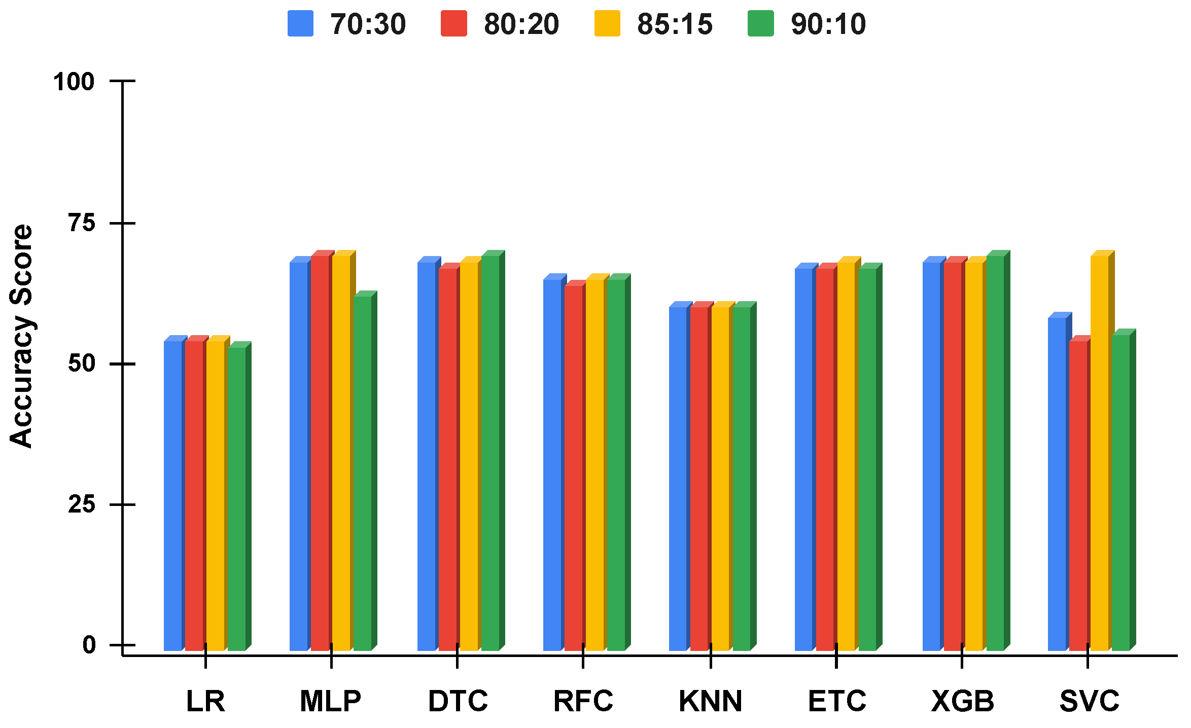
Figure 10.
The applied techniques performance comparative analysis of different data split ratios without proposed technique using imbalanced data.
Figure 10.
The applied techniques performance comparative analysis of different data split ratios without proposed technique using imbalanced data.
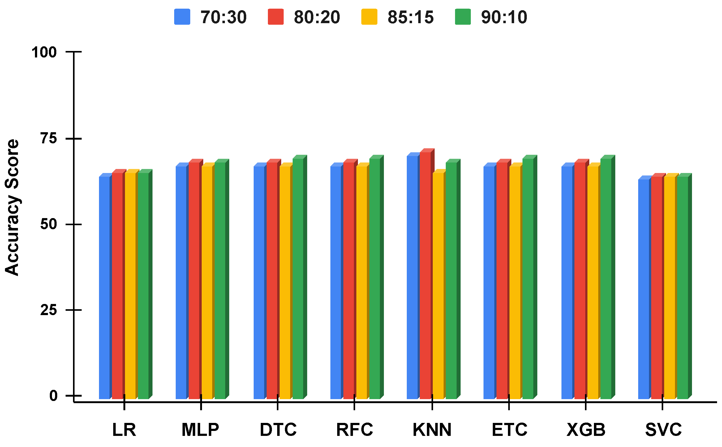
Figure 11.
The applied techniques performance comparative analysis of different data split ratios with proposed technique using imbalanced data.
Figure 11.
The applied techniques performance comparative analysis of different data split ratios with proposed technique using imbalanced data.
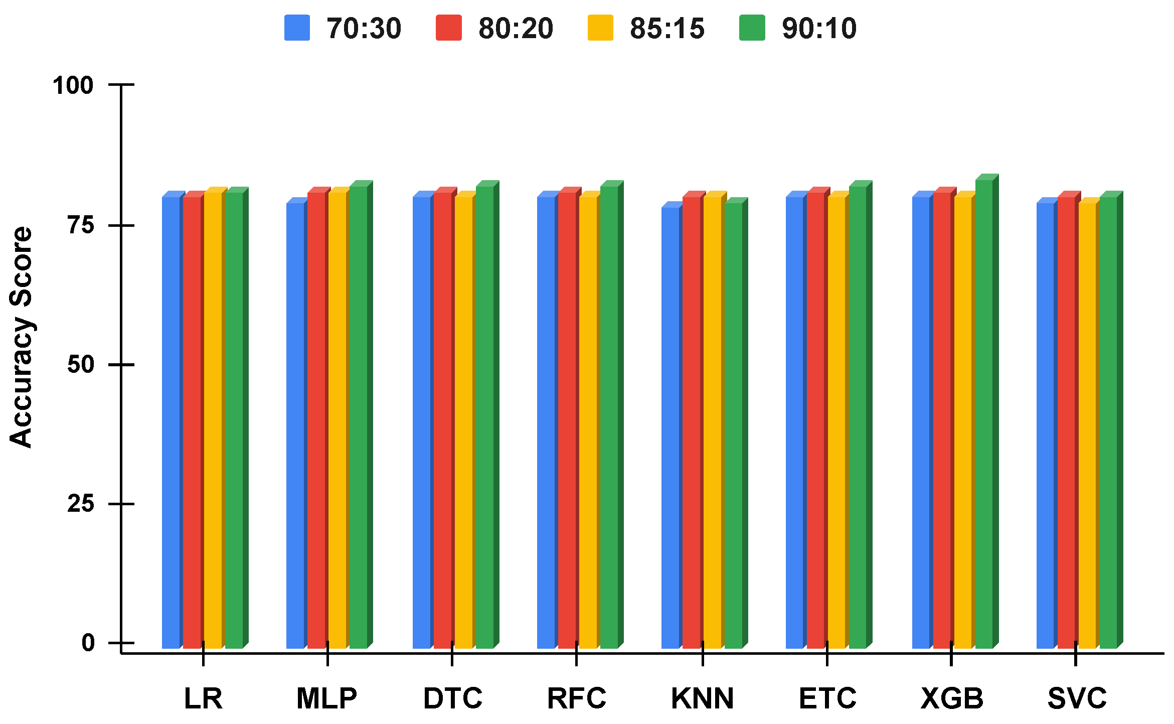
Figure 12.
The applied techniques performance comparative analysis of different data split ratios with proposed technique using balanced data.
Figure 12.
The applied techniques performance comparative analysis of different data split ratios with proposed technique using balanced data.
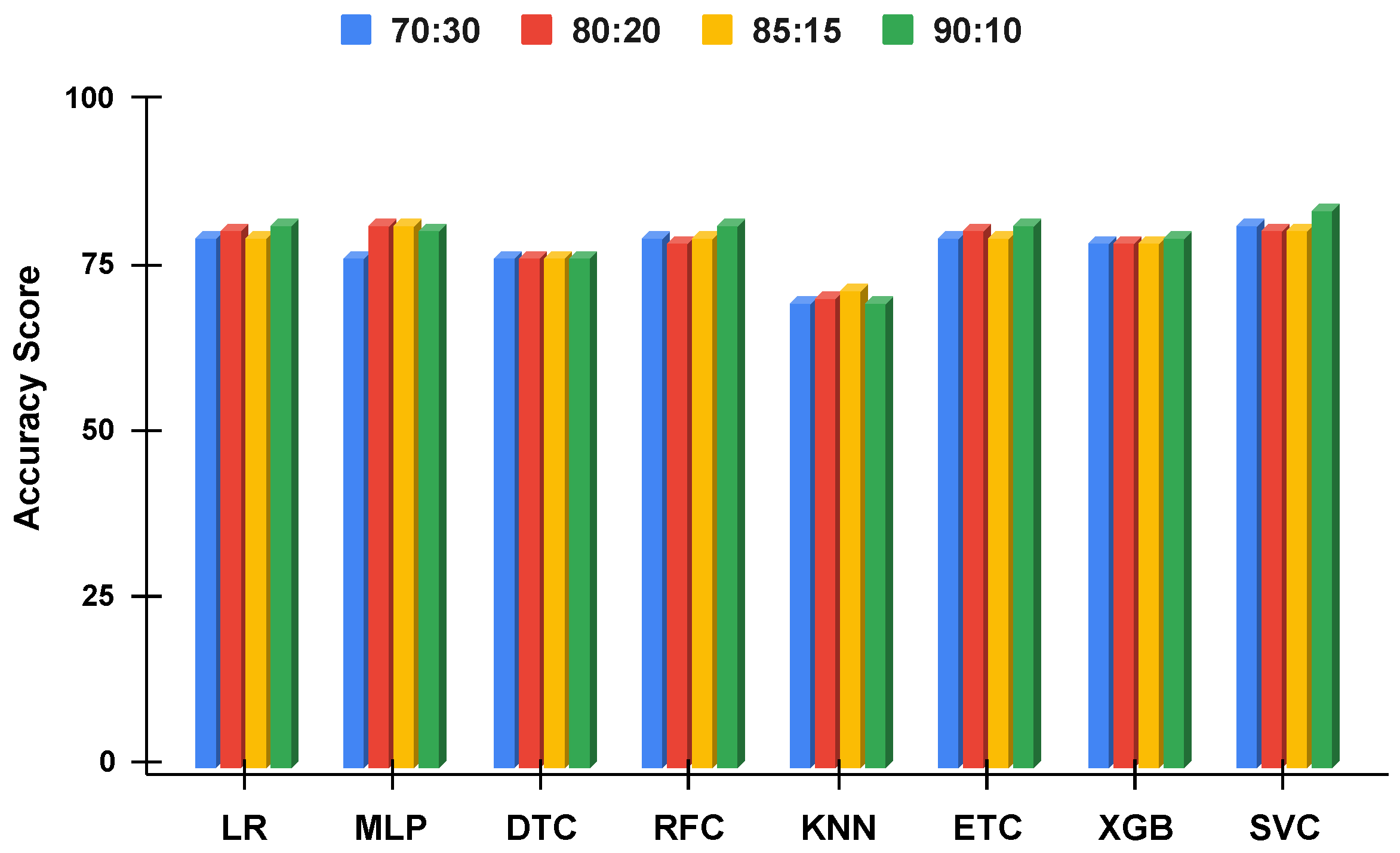
Figure 13.
The applied techniques performance comparative analysis of different data split ratios without proposed technique using balanced data.
Figure 13.
The applied techniques performance comparative analysis of different data split ratios without proposed technique using balanced data.
Table 1.
Summary of genetic disorder-related literature.
Table 1.
Summary of genetic disorder-related literature.
| Ref. | Year | Approach | Dataset | Accuracy (%) | Aim |
|---|
| [21] | 2021 | Stacked ML Model | AD genetic data of neuroimaging project (ADNI-1) | 93 | Classify Alzheimer’s disease type of brain disorders using ML. |
| [25] | 2021 | Genetic Disease Analyzer (GDA) | GEO dataset | 98 | Prediction of complex genes and identify genetic classifications that cause complex diseases. |
| [34] | 2021 | XGBoost | Alzheimer’s Disease Neuroimaging Initiatives (ADNI) | 64 | Alzheimer’s Disease Classification Using Genetic Data |
| [33] | 2020 | Machine Learning-based model | Genes data | - | Disease gene prediction using machine learning |
| [35] | 2020 | Machine Learning-based model | Microarray gene expression dataset of autism spectrum disorder (ASD) | 97 | Predicting autism spectrum disorder from associative genetic markers of phenotypic groups. |
| [36] | 2020 | Random forest classifier | GWAS and GTEx Portals data | 81 | Machine Learning-based Model for predicting the effect of the deleterious and neutral variant for Alzheimer’s disease. |
| [37] | 2021 | Support vector machine | Molecular-based network and brain connectome data | 72 | Propose a framework for integrating brain connectome data and molecular-based gene association networks to predict brain disease genes. |
| [27] | 2022 | Support vector machine | Multifactorial Genetic Inheritance Disorder multiclass dataset | 92 | Machine learning approaches were used to predict dementia, cancer, and diabetes. |
| [28] | 2021 | Random forest classifier | Metagenomic dataset-based on inflammatory bowel disease multi-omics | 90 | Inflammatory bowel disease prediction using machine learning techniques. |
| [29] | 2020 | Random forest classifier | Genetic SNP mutation dataset | 92 | Machine learning techniques were utilized to predict the COVID-19 infection and related diseases. |
| [30] | 2020 | Gradient boosting classifier | Virtual genetic, clinical test data | 83 | Prediction of familial hypercholesterolemia genetic disorder using the machine learning techniques. |
| [31] | 2017 | DOMINO | Genomic dataset | 92 | Machine learning-based DOMINO was used to Predict dominant mutations in Genes for Mendelian disorders. |
Table 2.
The genomes dataset features descriptive analysis.
Table 2.
The genomes dataset features descriptive analysis.
| Sr No. | Feature | Count | Data Type | Sr No. | Feature | Count | Data Type |
|---|
| 1 | Patient Id | 31,548 | object | 23 | Follow-up | 29,382 | object |
| 2 | Patient Age | 30,121 | float64 | 24 | Gender | 29,375 | object |
| 3 | Genes in mother’s side | 31,548 | object | 25 | Birth asphyxia | 29,409 | object |
| 4 | Inherited from father | 30,691 | object | 26 | Autopsy shows birth defect (if applicable) | 30,522 | object |
| 5 | Maternal gene | 25,015 | object | 27 | Place of birth | 29,424 | object |
| 6 | Paternal gene | 31,548 | object | 28 | Folic acid details (peri-conceptional) | 29,431 | object |
| 7 | Blood cell count (mcL) | 31,548 | float64 | 29 | H/O serious maternal illness | 29,396 | object |
| 8 | Patient First Name | 31,548 | object | 30 | H/O radiation exposure (X-ray) | 29,395 | object |
| 9 | Family Name | 12,540 | object | 31 | H/O substance abuse | 29,353 | object |
| 10 | Father’s name | 31,548 | object | 32 | Assisted conception IVF/ART | 29,426 | object |
| 11 | Mother’s age | 25,512 | float64 | 33 | History of anomalies in previous pregnancies | 29,376 | object |
| 12 | Father’s age | 25,562 | float64 | 34 | No. of previous abortion | 29,386 | float64 |
| 13 | Institute Name | 24,406 | object | 35 | Birth defects | 29,394 | object |
| 14 | Location of Institute | 31,548 | object | 36 | White Blood cell count (thousand per microliter) | 29,400 | float64 |
| 15 | Status | 31,548 | object | 37 | Blood test result | 29,403 | object |
| 16 | Respiratory Rate (breaths/min) | 26,513 | object | 38 | Symptom 1 | 29,393 | object |
| 17 | Heart Rate (rates/min | 26,535 | object | 39 | Symptom 2 | 29,326 | object |
| 18 | Test 1 | 29,421 | float64 | 40 | Symptom 3 | 29,447 | object |
| 19 | Test 2 | 29,396 | float64 | 41 | Symptom 4 | 29,435 | object |
| 20 | Test 3 | 29,401 | float64 | 42 | Symptom 5 | 29,395 | object |
| 21 | Test 4 | 29,408 | float64 | 43 | Genetic Disorder | 19,937 | object |
| 22 | Test 5 | 29,378 | float64 | 44 | Disorder Subclass | 19,915 | object |
Table 3.
Configuration of hyperparameters for employed machine learning models.
Table 3.
Configuration of hyperparameters for employed machine learning models.
| Technique | Hyperparameters |
|---|
| ETC | n_estimators = 300, random_state = 5, max_depth = 300, criterion = “gini”, max_features = “sqrt”, bootstrap = False, oob_score = False, ccp_alpha = 0.0 |
| SVC | penalty = ‘l2’, loss = ‘squared_hinge’, tol = 1 × 10⁻⁴, C = 1.0, multi_class = ‘ovr’, fit_intercept = True, max_iter = 1000 |
| LR | penalty =‘l2’, tol = 1 × 10⁻⁴, C = 1.0, fit_intercept = True, solver = ‘lbfgs’, random_state = None, max_iter = 100, multi_class = ‘auto’ |
| DTC | max_depth = 300, criterion = “gini”, splitter = “best”, ccp_alpha = 0.0, random_state = None |
| RFC | max_depth = 300, n_estimatorsint = 100, criterion = “gini”, max_features = “sqrt”, random_state = None, bootstrap = True, ccp_alpha = 0.0 |
| XGB | use_label_encoder = False, eval_metric = ‘mlogloss’, max_depth = 300, objective = ‘multi:softprob’ |
| KNN | n_neighbors = 5, weights = ‘uniform’, leaf_size = 30, metric = ‘minkowski’, algorithm = ‘auto’, p = 2 |
| MLP | hidden_layer_sizes = 100, max_iter = 300, activation = ‘relu’, solver = ‘adam’, alpha = 0.0001, learning_rate = ‘constant’, tol = 1 × 10⁻⁴, epsilon = 1 × 10⁻⁸, max_fun = 15000 |
Table 4.
Comparative analysis of machine learning models using an unbalanced dataset with a data split of 70:30.
Table 4.
Comparative analysis of machine learning models using an unbalanced dataset with a data split of 70:30.
| Technique | Label 1 | Label 2 |
|---|
| Results without Proposed Technique |
|---|
| Accuracy (%) | Precision (%) | Recall (%) | F1 Score (%) | Accuracy (%) | Precision (%) | Recall (%) | F1 Score (%) |
|---|
| LR | 53 | 51 | 42 | 36 | 33 | 19 | 17 | 14 |
| MLP | 58 | 52 | 51 | 50 | 35 | 26 | 25 | 24 |
| DTC | 50 | 44 | 44 | 44 | 29 | 23 | 24 | 24 |
| RFC | 58 | 54 | 46 | 46 | 37 | 28 | 22 | 23 |
| KNN | 46 | 36 | 34 | 33 | 21 | 13 | 12 | 12 |
| ETC | 59 | 54 | 48 | 49 | 37 | 40 | 24 | 26 |
| XGB | 57 | 51 | 49 | 49 | 36 | 30 | 25 | 26 |
| SVC | 49 | 48 | 35 | 34 | 27 | 20 | 14 | 12 |
| | Results with Proposed Technique |
| LR | 64 | 73 | 69 | 66 | 43 | 39 | 38 | 36 |
| MLP | 66 | 74 | 72 | 71 | 45 | 58 | 41 | 40 |
| DTC | 66 | 74 | 72 | 71 | 44 | 51 | 41 | 41 |
| RFC | 66 | 74 | 72 | 71 | 44 | 51 | 41 | 41 |
| KNN | 53 | 67 | 67 | 65 | 35 | 38 | 40 | 37 |
| ETC | 66 | 74 | 72 | 71 | 44 | 51 | 41 | 41 |
| XGB | 66 | 74 | 72 | 71 | 44 | 51 | 41 | 41 |
| SVC | 64 | 73 | 69 | 65 | 42 | 35 | 38 | 36 |
Table 5.
The multi-label multi-class performance comparative analysis with an imbalanced dataset using a data split of 70:30.
Table 5.
The multi-label multi-class performance comparative analysis with an imbalanced dataset using a data split of 70:30.
| Technique | Training Time (s) | Macro Accuracy (%) | Hamming Loss | α-Evaluation Score |
|---|
| Results without the proposed technique |
| LR | 3.20 | 55 | 0.22 | 90 |
| MLP | 75.34 | 69 | 0.18 | 88 |
| DTC | 0.25 | 69 | 0.21 | 83 |
| RFC | 4.04 | 66 | 0.18 | 89 |
| KNN | 0.05 | 61 | 0.25 | 84 |
| ETC | 02.39 | 68 | 0.17 | 89 |
| XGB | 75.94 | 69 | 0.18 | 87 |
| SVC | 12.06 | 59 | 0.24 | 86 |
| Results with the proposed technique |
| LR | 2.05 | 65 | 0.18 | 91 |
| MLP | 13.17 | 68 | 0.18 | 90 |
| DTC | 0.01 | 68 | 0.17 | 90 |
| RFC | 0.79 | 68 | 0.17 | 90 |
| KNN | 0.02 | 71 | 0.23 | 78 |
| ETC | 2.18 | 68 | 0.17 | 90 |
| XGB | 7.49 | 68 | 0.17 | 90 |
| SVC | 0.28 | 64 | 0.18 | 91 |
Table 6.
Performance analysis of machine learning models using an imbalanced dataset with a data split of 80:20.
Table 6.
Performance analysis of machine learning models using an imbalanced dataset with a data split of 80:20.
| Technique | Label 1 | Label 2 |
|---|
| Results without Proposed Technique |
|---|
| Accuracy (%) | Precision (%) | Recall (%) | F1 Score (%) | Accuracy (%) | Precision (%) | Recall (%) | F1 Score (%) |
|---|
| LR | 53 | 52 | 42 | 37 | 33 | 19 | 17 | 14 |
| MLP | 60 | 54 | 50 | 51 | 37 | 27 | 24 | 25 |
| DTC | 49 | 43 | 43 | 43 | 29 | 21 | 21 | 21 |
| RFC | 58 | 54 | 45 | 45 | 36 | 27 | 21 | 22 |
| KNN | 47 | 36 | 34 | 34 | 22 | 12 | 12 | 12 |
| ETC | 59 | 55 | 48 | 49 | 37 | 34 | 23 | 25 |
| XGB | 57 | 52 | 48 | 49 | 36 | 32 | 26 | 28 |
| SVC | 50 | 45 | 35 | 32 | 19 | 17 | 16 | 12 |
| | Results with Proposed Technique |
| LR | 65 | 75 | 71 | 68 | 43 | 39 | 39 | 37 |
| MLP | 67 | 75 | 73 | 72 | 45 | 48 | 40 | 39 |
| DTC | 67 | 75 | 73 | 72 | 45 | 55 | 41 | 41 |
| RFC | 67 | 75 | 73 | 72 | 45 | 54 | 41 | 40 |
| KNN | 55 | 69 | 69 | 66 | 37 | 43 | 42 | 40 |
| ETC | 67 | 75 | 73 | 72 | 45 | 55 | 41 | 41 |
| XGB | 67 | 75 | 73 | 72 | 45 | 55 | 41 | 41 |
| SVC | 65 | 75 | 70 | 67 | 43 | 40 | 38 | 36 |
Table 7.
The multi-label multi-class performance comparative analysis with an imbalanced dataset using a data split of 80:20.
Table 7.
The multi-label multi-class performance comparative analysis with an imbalanced dataset using a data split of 80:20.
| Technique | Training Time (s) | Macro Accuracy (%) | Hamming Loss | α-Evaluation Score |
|---|
| Results without the proposed technique |
| LR | 3.47 | 55 | 0.22 | 90 |
| MLP | 69.57 | 70 | 0.17 | 89 |
| DTC | 0.29 | 68 | 0.22 | 83 |
| RFC | 4.74 | 65 | 0.19 | 89 |
| KNN | 0.03 | 61 | 0.24 | 84 |
| ETC | 14.45 | 68 | 0.18 | 89 |
| XGB | 91.50 | 69 | 0.18 | 87 |
| SVC | 14.04 | 55 | 0.24 | 88 |
| Results with the proposed technique |
| LR | 2.16 | 66 | 0.17 | 91 |
| MLP | 10.95 | 69 | 0.16 | 90 |
| DTC | 0.01 | 69 | 0.16 | 90 |
| RFC | 0.88 | 69 | 0.16 | 90 |
| KNN | 0.03 | 72 | 0.26 | 79 |
| ETC | 2.44 | 69 | 0.16 | 90 |
| XGB | 9.13 | 69 | 0.16 | 90 |
| SVC | 0.34 | 65 | 0.17 | 92 |
Table 8.
Performance comparative analysis of models using an imbalanced dataset and 85:15 split.
Table 8.
Performance comparative analysis of models using an imbalanced dataset and 85:15 split.
| Technique | Label 1 | Label 2 |
|---|
| Results without Proposed Technique |
|---|
| Accuracy (%) | Precision (%) | Recall (%) | F1 Score (%) | Accuracy (%) | Precision (%) | Recall (%) | F1 Score (%) |
|---|
| LR | 54 | 52 | 42 | 37 | 32 | 15 | 16 | 13 |
| MLP | 61 | 55 | 53 | 53 | 38 | 30 | 29 | 29 |
| DTC | 51 | 44 | 44 | 44 | 30 | 24 | 25 | 24 |
| RFC | 58 | 54 | 46 | 46 | 36 | 27 | 21 | 22 |
| KNN | 47 | 33 | 33 | 32 | 22 | 13 | 13 | 12 |
| ETC | 59 | 54 | 47 | 48 | 37 | 33 | 23 | 25 |
| XGB | 57 | 51 | 48 | 49 | 35 | 27 | 23 | 24 |
| SVC | 41 | 44 | 34 | 29 | 25 | 20 | 20 | 14 |
| | Results with Proposed Technique |
| LR | 65 | 75 | 70 | 67 | 42 | 40 | 38 | 36 |
| MLP | 66 | 74 | 72 | 71 | 43 | 45 | 40 | 39 |
| DTC | 66 | 74 | 72 | 70 | 42 | 47 | 40 | 40 |
| RFC | 66 | 74 | 72 | 71 | 43 | 48 | 40 | 40 |
| KNN | 65 | 74 | 70 | 68 | 39 | 44 | 38 | 38 |
| ETC | 66 | 74 | 72 | 70 | 42 | 47 | 40 | 40 |
| XGB | 66 | 74 | 72 | 71 | 42 | 45 | 39 | 39 |
| SVC | 64 | 74 | 70 | 66 | 41 | 35 | 38 | 35 |
Table 9.
The multi-label multi-class performance comparative analysis with an imbalanced dataset using a data split of 85:15.
Table 9.
The multi-label multi-class performance comparative analysis with an imbalanced dataset using a data split of 85:15.
| Technique | Training Time (s) | Macro Accuracy (%) | Hamming Loss | α-Evaluation Score |
|---|
| Results without the proposed technique |
| LR | 4.08 | 55 | 0.22 | 91 |
| MLP | 104.1 | 70 | 0.16 | 89 |
| DTC | 0.31 | 69 | 0.21 | 84 |
| RFC | 5.42 | 66 | 0.18 | 89 |
| KNN | 0.04 | 61 | 0.25 | 84 |
| ETC | 16.8 | 69 | 0.18 | 89 |
| XGB | 99.37 | 69 | 0.18 | 87 |
| SVC | 16.4 | 70 | 0.25 | 77 |
| Results with the proposed technique |
| LR | 2.49 | 66 | 0.17 | 92 |
| MLP | 13.58 | 68 | 0.17 | 90 |
| DTC | 0.01 | 68 | 0.17 | 90 |
| RFC | 0.95 | 68 | 0.17 | 90 |
| KNN | 0.03 | 66 | 0.17 | 91 |
| ETC | 2.55 | 68 | 0.17 | 90 |
| XGB | 9.40 | 68 | 0.17 | 90 |
| SVC | 0.38 | 65 | 0.18 | 92 |
Table 10.
Performance comparative analysis using an imbalanced dataset with a data split of 90:10.
Table 10.
Performance comparative analysis using an imbalanced dataset with a data split of 90:10.
| Technique | Label 1 | Label 2 |
|---|
| Results without Proposed Technique |
|---|
| Accuracy (%) | Precision (%) | Recall (%) | F1 Score (%) | Accuracy (%) | Precision (%) | Recall (%) | F1 Score (%) |
|---|
| LR | 53 | 57 | 42 | 37 | 34 | 24 | 17 | 14 |
| MLP | 57 | 56 | 49 | 48 | 36 | 31 | 24 | 24 |
| DTC | 50 | 44 | 45 | 44 | 30 | 23 | 24 | 24 |
| RFC | 58 | 56 | 46 | 47 | 38 | 39 | 23 | 25 |
| KNN | 46 | 34 | 33 | 32 | 22 | 13 | 12 | 12 |
| ETC | 59 | 56 | 48 | 49 | 38 | 40 | 26 | 28 |
| XGB | 57 | 52 | 49 | 50 | 36 | 33 | 26 | 28 |
| SVC | 51 | 40 | 41 | 35 | 31 | 15 | 19 | 15 |
| | Results with Proposed Technique |
| LR | 66 | 77 | 71 | 68 | 43 | 40 | 38 | 37 |
| MLP | 67 | 76 | 73 | 71 | 45 | 45 | 40 | 40 |
| DTC | 67 | 76 | 73 | 72 | 45 | 50 | 41 | 41 |
| RFC | 67 | 76 | 73 | 73 | 45 | 51 | 41 | 41 |
| KNN | 62 | 71 | 71 | 70 | 41 | 50 | 42 | 42 |
| ETC | 67 | 76 | 73 | 72 | 45 | 50 | 41 | 41 |
| XGB | 67 | 76 | 73 | 72 | 45 | 50 | 42 | 42 |
| SVC | 65 | 76 | 70 | 66 | 43 | 41 | 38 | 36 |
Table 11.
The multi-label multi-class performance comparative analysis using a data split of 90:10.
Table 11.
The multi-label multi-class performance comparative analysis using a data split of 90:10.
| Technique | Training Time (s) | Macro Accuracy (%) | Hamming Loss | α-Evaluation Score |
|---|
| Results without the proposed technique |
| LR | 5.23 | 54 | 0.22 | 91 |
| MLP | 40.5 | 63 | 0.19 | 90 |
| DTC | 0.33 | 70 | 0.20 | 84 |
| RFC | 5.70 | 66 | 0.18 | 90 |
| KNN | 0.04 | 61 | 0.25 | 84 |
| ETC | 17.62 | 68 | 0.18 | 89 |
| XGB | 106.58 | 70 | 0.18 | 88 |
| SVC | 19.0 | 56 | 0.23 | 90 |
| Results with the proposed technique |
| LR | 2.76 | 66 | 0.17 | 92 |
| MLP | 17.6 | 69 | 0.16 | 91 |
| DTC | 0.01 | 70 | 0.16 | 90 |
| RFC | 1.02 | 70 | 0.16 | 90 |
| KNN | 0.03 | 69 | 0.19 | 87 |
| ETC | 2.82 | 70 | 0.16 | 90 |
| XGB | 15.7 | 70 | 0.16 | 90 |
| SVC | 0.37 | 65 | 0.17 | 92 |
Table 12.
Comparative analysis of applied machine learning models using a balanced dataset with a data split of 80:20.
Table 12.
Comparative analysis of applied machine learning models using a balanced dataset with a data split of 80:20.
| Technique | Label 1 | Label 2 |
|---|
| Results without Proposed Technique |
|---|
| Accuracy (%) | Precision (%) | Recall (%) | F1 Score (%) | Accuracy (%) | Precision (%) | Recall (%) | F1 Score (%) |
|---|
| LR | 55 | 54 | 56 | 54 | 41 | 18 | 22 | 19 |
| MLP | 58 | 57 | 58 | 57 | 41 | 26 | 24 | 24 |
| DTC | 47 | 47 | 47 | 47 | 32 | 24 | 26 | 25 |
| RFC | 57 | 56 | 57 | 55 | 42 | 23 | 23 | 21 |
| KNN | 37 | 37 | 37 | 36 | 25 | 14 | 14 | 14 |
| ETC | 58 | 57 | 58 | 57 | 43 | 47 | 26 | 26 |
| XGB | 54 | 53 | 54 | 53 | 39 | 41 | 26 | 27 |
| SVC | 37 | 44 | 37 | 027 | 25 | 20 | 20 | 15 |
| | Results with Proposed Technique |
| LR | 72 | 73 | 73 | 72 | 57 | 38 | 41 | 39 |
| MLP | 74 | 74 | 74 | 73 | 51 | 59 | 42 | 41 |
| DTC | 73 | 73 | 73 | 73 | 59 | 50 | 45 | 44 |
| RFC | 73 | 73 | 73 | 73 | 59 | 50 | 44 | 44 |
| KNN | 71 | 71 | 71 | 71 | 56 | 44 | 44 | 44 |
| ETC | 73 | 73 | 73 | 73 | 59 | 50 | 44 | 44 |
| XGB | 73 | 73 | 73 | 73 | 59 | 49 | 44 | 44 |
| SVC | 72 | 73 | 73 | 72 | 38 | 58 | 41 | 39 |
Table 13.
The multi-label multi-class performance comparative analysis using balanced data with 80:20 split.
Table 13.
The multi-label multi-class performance comparative analysis using balanced data with 80:20 split.
| Technique | Training Time (s) | Macro Accuracy (%) | Hamming Loss | α-Evaluation Score |
|---|
| Results without the proposed technique |
| LR | 0.99 | 81 | 0.16 | 87 |
| MLP | 17.21 | 82 | 0.14 | 89 |
| DTC | 0.08 | 77 | 0.19 | 87 |
| RFC | 1.63 | 79 | 0.16 | 89 |
| KNN | 0.01 | 71 | 0.24 | 85 |
| ETC | 4.54 | 81 | 0.14 | 90 |
| XGB | 19.98 | 79 | 0.17 | 88 |
| SVC | 3.41 | 81 | 0.17 | 82 |
| Results with the proposed technique |
| LR | 0.50 | 81 | 0.14 | 91 |
| MLP | 6.81 | 82 | 0.14 | 91 |
| DTC | 0.01 | 82 | 0.14 | 89 |
| RFC | 0.54 | 82 | 0.14 | 89 |
| KNN | 0.01 | 81 | 0.15 | 88 |
| ETC | 1.32 | 82 | 0.14 | 89 |
| XGB | 3.32 | 82 | 0.14 | 89 |
| SVC | 0.09 | 81 | 0.14 | 91 |
Table 14.
Results for the proposed XGB as classification model for multi-omics and high dimensional real genomic dataset.
Table 14.
Results for the proposed XGB as classification model for multi-omics and high dimensional real genomic dataset.
| Category | Precision | Recall | F1 Score |
|---|
| 0 | 1.00 | 1.00 | 1.00 |
| 1 | 1.00 | 1.00 | 1.00 |
| 2 | 1.00 | 1.00 | 1.00 |
| 3 | 1.00 | 1.00 | 1.00 |
| 4 | 1.00 | 1.00 | 1.00 |
| Average | 1.00 | 1.00 | 1.00 |
| Accuracy | 1.00 |
Table 15.
Comparative analysis of proposed approach with state-of-the-art approaches.
Table 15.
Comparative analysis of proposed approach with state-of-the-art approaches.
| Reference | Year | Technique | Training Time (s) | Macro Accuracy (%) | Hamming Loss | -Evaluation Score (%) |
|---|
| [63] | 2020 | SVM | 7.10 | 73 | 0.22 | 88 |
| [64] | 2020 | KNN | 0.01 | 70 | 0.25 | 86 |
| [65] | 2020 | KNN | 0.01 | 70 | 0.25 | 86 |
| [66] | 2020 | RF | 2.48 | 82 | 0.14 | 90 |
| [67] | 2021 | KNN | 0.01 | 70 | 0.25 | 86 |
| Proposed | 2022 | ETRF + XGB | 3.59 | 84 | 0.12 | 92 |


 ,
, 


