Assessment of the Standardized Precipitation and Evaporation Index (SPEI) as a Potential Management Tool for Grasslands

Abstract

Early warning of detrimental weather and climate (particularly drought) on forage production would allow for tactical decision-making for the management of pastures, supplemental feed/forage resources, and livestock. The standardized precipitation and evaporation index (SPEI) has been shown to be correlated with production of various cereal and vegetable crops, and with above-ground tree mass. Its correlation with above-ground grassland or forage mass (AGFM) is less clear. To investigate the utility of SPEI for assessing future biomass status, we used biomass data from a site on the Konza Prairie (KP; for years 1984–1991) and from a site at the United States Department of Agriculture-Agricultural Research Service’s (USDA-ARS) Grazinglands Research Laboratory (GRL; for years 2009–2015), and a publicly-available SPEI product. Using discriminant analysis and artificial neural networks (ANN), we analyzed the monthly timescale SPEI to categorize AGFM into above average, average, and below average conditions for selected months in the grazing season. Assessment of the confusion matrices from the analyses suggested that the ANN better predicted class membership from the SPEI than did the discriminant analysis. Within-site cross validation of the ANNs revealed classification errors ranging from 0 to 50%, depending upon month of class prediction and study site. Across-site ANN validation indicated that the GRL ANN algorithm better predicted KP AGFM class membership than did the KP ANN prediction of GRL AGFM class membership; however, misclassification rates were ≥25% in all months. The ANN developed from the combined datasets exhibited cross-validation misclassification rates of ≤20% for three of the five months being predicted, with the remaining two months having misclassification rates of 33%. Redefinition of the AGFM classes to identify truly adequate AGFM (i.e., average to above average forage availability) improved prediction accuracy. In this regard, results suggest that the SPEI has potential for use as a predictive tool for classifying AGFM, and, thus, for grassland and livestock management. However, a more comprehensive investigation that includes a larger dataset, or combinations of datasets representing other areas, and inclusion of a bi-weekly SPEI may provide additional insights into the usefulness of the SPEI as an indicator for biomass production.

1. Introduction

Forage-based agricultural systems in the US Southern Plains (SP) states of Kansas, Oklahoma, and Texas are vulnerable to climate extremes, especially drought [1]. According to References [2,3,4], the beef cattle industry in these states accounted for ~$26 billion US in total agricultural sales in 2012. With respect to US cattle production, Texas, Kansas, and Oklahoma ranked 1, 3, and 5, respectively, in production of all cattle in 2017 [5]. Combined, these states accounted for 21.3 million head of cattle and contained 55 million ha of grass and range lands in 2012 [2,3,4]. As with most other agricultural systems, extremes in weather conditions can adversely impact production. For example, the drought of 2011 caused ~$7.6 US billion in agricultural losses in Texas alone [6]. Early warning of potential detrimental effects of weather and climate (particularly drought) on forage production would allow for tactical decision-making for the management of pastures and/or livestock (e.g., timely implementation of pasture rotations, adjustment of stocking density, advanced notice of possible needs of earlier supplemental feeding, or acquisition of additional forage resources).

Precipitation, soil water content, and evapotranspiration (ET) are key variables affecting crop yield and biomass production. The amount and timing of rainfall in relation to plant development clearly has an impact on crop yields and biomass production [7,8,9]. However, not all precipitation successfully infiltrates the soil, and that which does may percolate to depths beyond the reach of plant root systems. Many investigators have also shown that the amount of soil water greatly affects crop yield [10,11,12] and other grain crops and grasslands [13], but such measurements are not routinely collected and recorded at most locations.

Over the last several decades, numerous indices and indicators of drought have been developed to assess the onset/end, extent, and severity of drought. These indices or indicators may be classified as meteorological (e.g., the Palmer Drought Severity Index [14] and the Standardized Precipitation Index (SPI) [15]); may be designed to reflect soil moisture conditions (e.g., Soil Moisture Anomaly [16]) or the status of surface hydrology (e.g., the Standardized Streamflow Index [17]); or may be based on remotely sensed data (e.g., the Evaporative Stress Index [18]). A more complete listing of indicators may be found in References [19]. The standardized precipitation and evaporation index (SPEI, [20]), which builds upon the methodology used to develop the SPI, is a water-balance drought index based on the difference between precipitation (water supply) and potential evapotranspiration (ETp, water demand). It has been suggested that the SPEI may be functional for assessment of agricultural drought and, hence, biomass production [21,22]. Values of the SPEI may be positive (wet conditions) or negative (dry conditions), and are interpreted as the number of standard deviations away from the mean conditions. The SPEI is scalable over time periods of 1 to 48 months (or longer). For example, a 3 month SPEI value calculated for June (i.e., 3SPEI6) would represent the number of standard deviations (+/−) from the mean for the April–June time period. This scalability allows assessment of the cumulative effects of local weather/climate for time periods of various lengths.

The 1 month SPEI has been shown to closely follow the decline in soil water content, gross primary productivity, and ET measured for maize grown near Mead, NE, USA [23], and 1, 3, and 6 month timescale SPEIs were found to correlate well with biomass production for several different climate/vegetation regimes [24]. Several drought indices were evaluated by Reference [25], and the revised SPEI with crop-specific potential ET was found to follow the trends and magnitudes of water demand for several irrigated summer crops grown in the Texas High Plains in the USA. A linear regression model, based on a time-series of SPEI (April through September) values, accounted for ≈59% of the variability in yield for several vegetable crops for a study site in the Czech Republic [26]. This study was followed by another assessment [27], and it was shown that the SPEI, computed at various time scales, was correlated with productivity for 11 different crops grown in the Czech Republic. These investigators [27] found that the correlations between the SPEI and crop productivity were different for each crop and for different SPEI timescales, with the greatest correlation (r) achieved for cereal crops (r = 0.52–0.60; for a monthly timescale SPEI for the months May and June). Above-ground deciduous tree biomass for Mediterranean forests correlated significantly (r = 0.55 and 0.67, respectively) with the September and December SPEI [28] for Mediterranean forests, and it was shown that the interannual variability of above-ground tree (evergreen) mass in the Swiss Alps was also correlated with SPEI [29]. In terms of grassland above-ground mass, correlation has been reported between the 3, 6, 12, and 24 month timescale SPEI and grassland production in China [30], and it was shown that the monthly scale SPEI for July through September was better related to biomass production for grasslands and shrublands than SPEIs at other timescales [31]. However, Reference [32] assessed the SPEI’s sensitivity to drought for six grasslands in the central US, and found no statistically significant relationships. These investigators also indicated that legacy effects of the previous (calendar) year’s rainfall contributed little to biomass production in the following year. This lack of impact of the previous year’s rainfall on the following year’s biomass production was also noted for grasslands in central Oklahoma, USA [33,34].

Given the inconsistent results noted in the literature, and the probability of non-significant legacy effects of the previous calendar year’s rainfall on grassland biomass production, we further examined the relationship of SPEI with grassland production in the Southern Plains of the US. More specifically, our objectives were: (1) to determine if the monthly-scale SPEIs obtained in the early part of the calendar year can be used to classify above-ground forage biomass (AGFM) into above average, below average, and average conditions for months later in the grazing season, and (2) to determine if successful assessment at one location can be directly applied to another location with similar forage and climatic conditions. If successful, application of the SPEI in this way could provide an early warning of probable shortfalls in forage production for grassland and livestock managers, and may be useful as a grassland management tool.

2. Materials and Methods

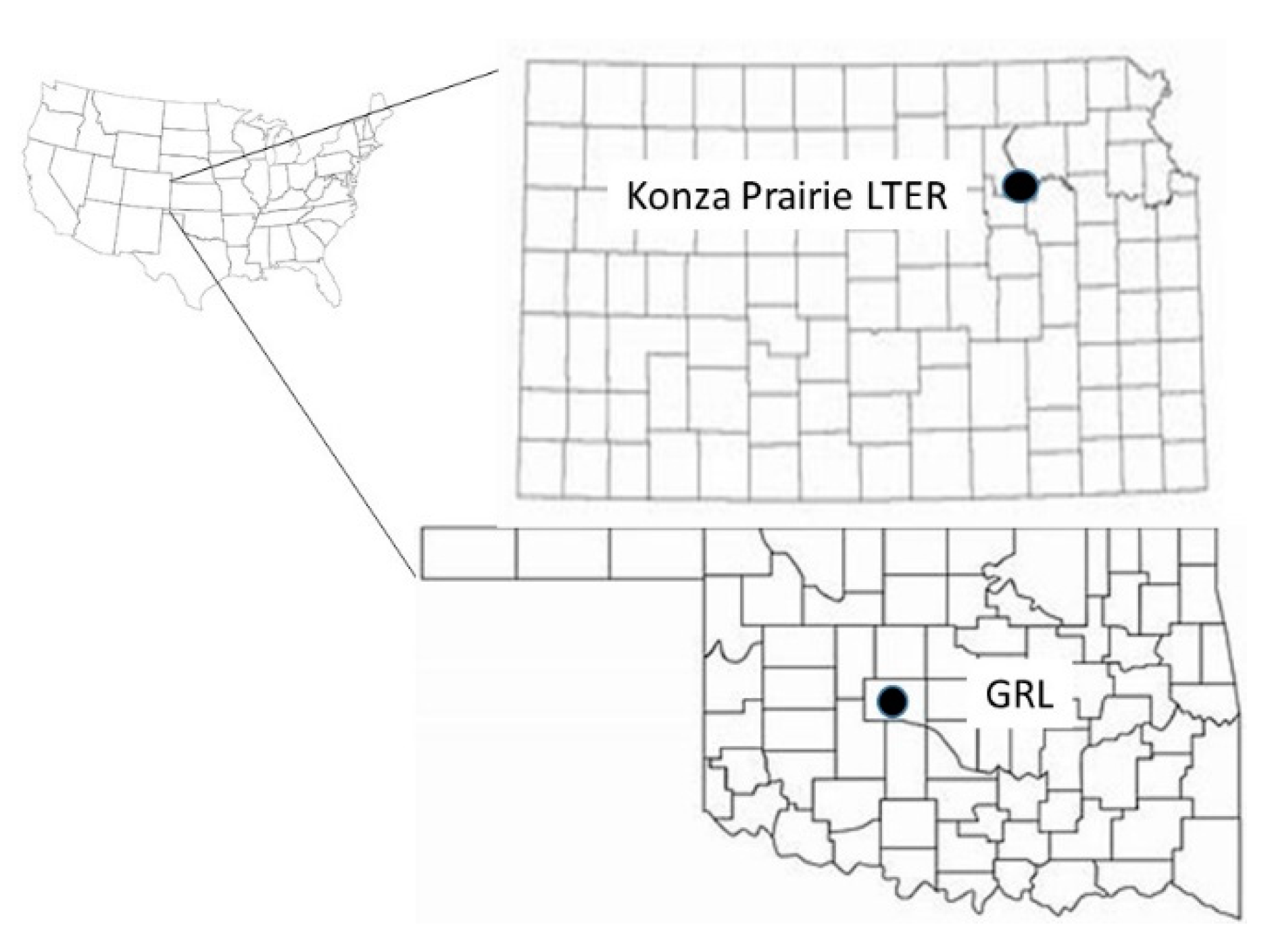
2.1. Study Sites

The study was conducted using data collected at Konza Prairie (KP) Long-Term Ecological Research site near Manhattan, Kansas, USA (39°06′0.38″ N, 96°36′29.5″ W), and at the US Department of Agriculture’s Agricultural Research Service Grazinglands Research Laboratory (GRL), located in El Reno, Oklahoma, USA (35°33′29″ N, 98°01′50″ W) (Figure 1). The two sites are similar in that they both belong to the Level 1 (Great Plains) and Level 2 (South Central Semi-Arid Prairie) ecoregions, as defined by the US Environmental Protection Agency (https://www.epa.gov/eco-research/ecoregions-north-america). Additionally, both sites fall within the Koeppen–Geiger (http://koeppen-geiger.vu-wien.ac.at/usa.htm) Cfa climate classification (warm temperate, fully humid, hot summer). The 30 year (1981–2010) annual average (“normal”) rainfall at the KP is ~904 mm, and ~913 mm at the GRL. The normal maximum air temperatures at the KP and GRL in January and July are 5 and 33.3, and 9.0 and 34.1 °C, respectively (data available at https://www. ncdc.novv.gov/normalsPDFaccess/). Warm season perennial grasses dominate both sites, with the most abundant being big bluestem (Andropogon gerardii Vtiman), little bluestem (Schizacyrium scoparium, (Michx.) Nash), Indiangrass (Sorghastrum nutans (L.) Nash), and switchgrass (Pancium virgatum, L.). The terrain at the KP is hilly, but is gently rolling at the GRL.

Established as a research site in 1971, the KP is 3487 ha in size and is the largest area of unplowed prairie in North America. The KP has been divided into numerous watershed units which receive various management treatments (e.g., grazed vs. ungrazed; prescribed burn frequency, patch burning), and provides a rich data source (including AGFM) related to tallgrass prairies. (See http://lter.konza.ksu.edu/ for a more complete site description and for data access and collection protocols.)

The AGFM data from the GRL was collected during a grazing study initiated in 2009 on 346 ha of native tallgrass prairie grasses, divided into two control paddocks of ~63 ha each and two rotational units of ~83 ha each. The control paddocks were assigned to continuous year-round stocking. The rotational units were divided into 10 approximately equally-sized sub-paddocks. The cattle in these sub-units were moved on a weekly basis. (For specifics on experimental design, stocking rates, etc. see Reference [34].) From 1949 to 2008, the site was primarily subjected to year-round continuous stocking by beef cattle.

2.2. Above-Ground Forage Mass

For the purposes of this study, and to minimize the confounding effects of grazing on AGFM classification, the AGFM data used herein reflect ungrazed conditions.

The AGFM data for the KP were acquired from their website (http://lter.konza.ksu.edu/data) from the dataset labeled PAB02 [35]. The AGFM data selected from PAB02 were collected on watershed 000a (KP000a), and represent bi-weekly harvests for the years 1984–1991 and for the months May through September. The samples were collected from five 0.1 m² areas (clipped to ground level) spaced 10 m apart along four transects (n = 20 per watershed per sampling date) and reflect ungrazed and unburned conditions. To ensure that areas were not re-sampled, subsequent sampling occurred “one step” away from and parallel to the previously sampled transect. The AGFM data used from the KP were provided on a g m⁻² on a dry weight basis. The bi-weekly samples (n = 40) for a given month and year were averaged and converted to kg ha⁻¹ to represent the AGFM for that month within that year (one value for each month for each year), yielding eight biomass observations per month.

The AGFM data for the GRL were collected from 2009 through 2015. Within the continuously stocked pastures, biomass samples were collected semi-monthly (May through September) at four random locations in areas visually identified as not having been grazed within the May through September timeframe of the current calendar year. Within the rotational units, biomass was collected (May through September) at two random locations within and prior to (or at the time of) the introduction of the cattle into the sub-units. All biomass samples were collected within a sampling area measuring 0.5 m² and were harvested to within 1 cm of the soil surface. The samples were weighed fresh, then dried in a forced-air oven at 65 °C for 48 h, then weighed dry to determine dry AGFM. The biomass measurements for a given month and year from both the continuously stocked and rotational sub-units were averaged to provide a monthly value for each year of study. This averaging resulted in seven biomass observations per month (one observation for each month for each of the seven years of study).

The monthly AGFM data from KP000a and GRL were tested for normality using the Shapiro–Wilk’s W-test [36] (α = 0.05). Those data not meeting the normality test were further examined for outliers using box plots, and, if found, were removed from the dataset and re-analyzed for normality. Any remaining non-normal AGFM distributions were transformed using a Johnson Sb transformation [37]. Normally distributed monthly biomass values were assigned to the appropriate AGFM class based on the upper and lower 95% confidence intervals of the respective monthly means. Non-normally distributed monthly biomass values were first transformed using the Johnson Sb transformation, and then assigned to the appropriate AGFM class based on the upper and lower 95% confidence intervals of the mean of the transformed data. In all cases, the monthly values above the upper 95% confidence interval were designated as “above average” (abv), those biomass values below the lower 95% confidence interval were designated “below average” (blw), and all other values were designated “average” (avg).

Assuming that the month of September represents peak biomass, within-site annual variability in peak biomass was examined via plots of biomass and Tukey’s Honestly Significant Difference (HSD, α = 0.05) [38] means test. Monthly variation in biomass values is depicted using box plots.

2.3. Standardized Precipitation and Evaporation Index (SPEI)

The SPEI was developed by Reference [20], and is a standardized value of the difference (D_i) of precipitation (P_i) and potential evapotranspiration (ETp_i) for month i:

$$D_i=P_i-ET{p}_i$$

(1)

The D_i values can be aggregated over different timescales, however the D_i are first standardized from a three-parameter log–logistic distribution:

$$f\left(x\right)= \frac{\beta }{\alpha }{\left(\frac{x-\gamma }{\alpha }\right)}^{\beta -1}\left(1+{\left(\frac{x-\gamma }{\alpha }\right)}^{\beta }\right)$$

(2)

The parameters α, β, and γ are calculated from probability-weighted moments (PWM) and used to determine the log–logistic distribution, which is applied to the D_i dataset. The SPEI is then calculated as the probability of exceeding a given value of D_i (W = −2 × ln(P)):

$$SPEI=W- \frac{C0+C1W+C2W^2}{1+d1W+d2W^2+d3W^3}$$

(3)

where C0, C1, C2, d1, d2, and d3 are constants. See References [19,35] for details.

For our study locations, we used the 0.5 degree gridded SPEI product, which was obtained from the Global SPEI database (https://climatedataguide.ucar.edu/climate-data/standardized-precipitation-evapotranspiration-index-spei). Latitude and longitude of the approximate centroid of each site were entered into the user interface, which returns the SPEI values for the grid point nearest to the input coordinates. In this dataset, SPEI is calculated using monthly precipitation and ET_p data provided by the Climatic Research Unit of the University of East Anglia, East Anglia, UK. For this product, ET_p is based on the FAO-56 Penman–Monteith equation [39] (http://spei.csic.es/database.html). Although the delivered product provides grid-specific SPEIs at timescales between 1 and 48 months, we only used the 1 month timescale.

Rather than calculate the SPEIs for each site, we chose to use this readily-available product for our study. A publicly-available SPEI represents the type of product that could be easily accessible and implemented for forecasting AGFM.

2.4. Statistical Analysis

We analyzed the ability of the 1 month SPEIs to be used as predictors for classifying AGFM into the abv, avg, and blw categories using discriminant analysis and artificial neural networks (ANN). Discriminant analysis is a multi-variate linear technique which seeks to separate observations into distinct classes based on a set of predictor variables (in this case, the SPEI values), and to assign new observations into previously defined groups [40]. All SPEI values for the months January through September, inclusive, were used to determine which months, if any, were most advantageous for AGFM classification. The objective functions used to evaluate the discriminant results included the overall misclassification rates and the confusion matrices. We used discriminant analysis and ANN in four ways: (1) we evaluated each site separately, by month, using the complete data; (2) we then separated the data for each site into calibration and validation datasets to test the calibrated discriminant function on data not used in the calibration phase; (3) we applied the site-specific discriminant and ANN functions developed for a given site in (1) to the other site to examine the transferability of the discriminant and ANN classification algorithm across sites; and (4) we combined the two datasets, from which we created calibration and validation datasets to determine if the accuracy of the resulting prediction algorithms increased. In (2) and (4), the validation datasets were based upon a random selection of the dataset that was first stratified according to the AGFM classes. This approach yielded 75% of the observations assigned to the calibration datasets, and the remaining 25% were assigned to the validation datasets. Misclassification rates for a given month were calculated by dividing the number of misclassified observations by the total number of observations for that month.

Artificial neural networks are non-linear, non-statistical mathematical models that mimic the learning process of the human brain [41]. The ANN does not assume normality of the data, nor is a minimum amount of data specified to develop a predictive algorithm. However, the number of hidden nodes, which provides the mathematical connection between the input neurons (in this case the monthly SPEI values) and the output neurons (one neuron in this case, the AGFM class), is constrained either as a function of the number of records in the dataset, or the number of input and output neurons, or a combination of these. For this study, the number of input neurons equaled four and the number of output neurons equaled one for both datasets. The number of records per month varied from six to eight, depending upon site and month. We set the number of hidden neurons to two (half of the sum of number of inputs and outputs), in accordance with Reference [41]. The ANN predictive algorithm is developed through weighting the neurons in the hidden layer, which is located between the input neurons and the output neurons. At the outset of running the ANN, every input neuron is connected to every hidden neuron, and every hidden neuron is connected to every output neuron. As the data records are read and evaluated by the ANN, the weights of the hidden neurons are adjusted so that inputs are associated as strongly as possible with the intended output neuron. The reading and evaluating of the dataset is done iteratively until the prediction ability of the ANN is maximized. The ANN used in this study is described as a fully connected multi-layer perceptron. We used the hyperbolic tangent transformation function between the input neurons and the hidden neurons. All analyses were performed in JMP 14 Pro (SAS Institute, Cary, NC, USA).

3. Results

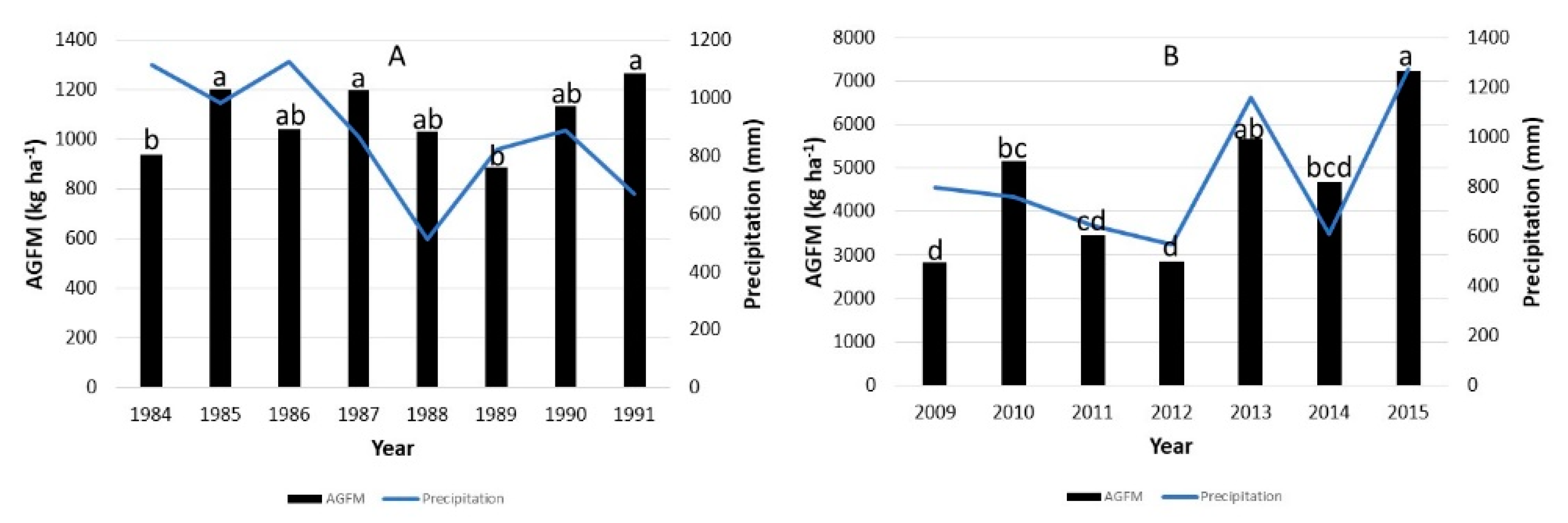
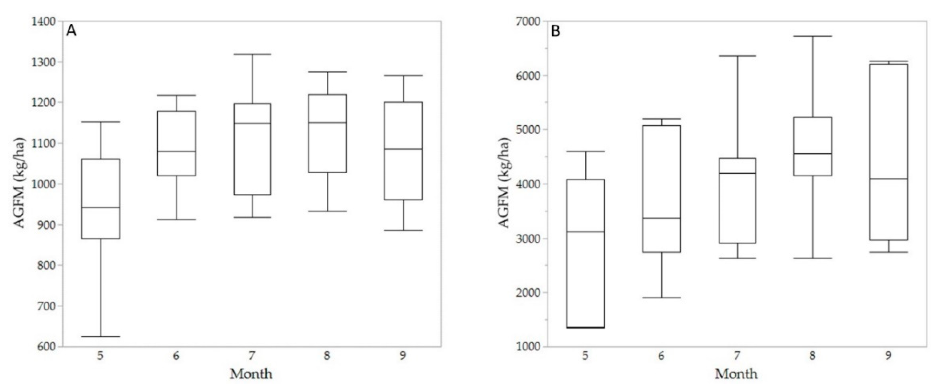
3.1. Above-Ground Forage Mass

No outliers were observed in the AGFM datasets. The Shapiro–Wilks W-test indicated that monthly biomass was normally distributed at KP000a; thus, the biomass data needed no transformation before assigning the AGFM values to the appropriate AGFM classes. However, the Shaprio–Wilks W-test indicated that the GRL biomass data for all months was not normally distributed. Therefore, these data were transformed before assignment to the appropriate AGFM class.

Assuming that September approximates peak biomass, it was observed (Figure 1) that AGFM varied by ~388 kg ha⁻¹ at KP000a, which is about 11 times smaller than the range in values observed at GRL. The AGFM values at KP000a were low compared to what has been reported (1500 to 5000 kg ha⁻¹) for other locations on the KP [42]. The cause of this low biomass production is not precisely known, but may relate to its not having been burned or grazed for many years, thus reducing the nutrient cycling necessary for plant growth. At KP000a, the highest observed AGFM occurred in 1991 (1265 kg ha⁻¹) and the lowest in 1989 (886 kg ha⁻¹). At GRL, the AGFM was 7230 kg ha⁻¹ in 2015 (Figure 2), which was statistically higher than all other years. The years 2009 and 2012 exhibited the lowest peak AGFM (~2800 kg ha⁻¹). It was also observed that considerable variation occurred in May at KP000a, while the variability was comparatively low and similar for the remaining months (Figure 3). AGFM at GRL was highly variable for all months.

3.2. Discriminant Analysis

Analysis of the entire site-specific datasets revealed that the 1 month timescale SPEIs representing months January through April (i.e., 1SPEI1–1SPEI4) were useful in differentiating AGFM classes at both sites (

Table 1. Misclassification rate results from the site-specific discriminant analysis of the 1 month time scale standardized precipitation and evaporation indices (SPEIs) and AGFM classifications for the Konza Prairie (KP000a) and GRL research sites. AGFM classifications are: abv = above average, avg = average, and blw = below average.

KP000a		Misclassification Rate 1			GRL		Misclassification Rate
SPEI Months	AGFM Month	abv	avg	blw	SPEI Months	AGFM Month	abv	avg	blw
1−4	May	0	17	0	1−4	May	0	0	0
	Jun	0	0	0		Jun	0	0	0
	Jul	0	0	0		Jul	0	-	0
	Aug	0	0	0		Aug	0	0	0
	Sep	0	0	0		Sep	33	0	0
1−5	Jun	0	0	0	1−5	Jun	0	0	0
	Jul	0	0	0		Jul	0	-	0
	Aug	0	0	0		Aug	33	0	0
	Sep	0	0	0		Sep	33	0	33
1−6	Jul	0	0	0	1−6	Jul	33	-	0
	Aug	0	0	0		Aug	33	50	0
	Sep	0	0	0		Sep	33	0	0
1−7	Aug	0	0	0	1−7	Aug	33	50	50
	Sep	0	0	0		Sep	33	0	0
1−8	Sep	0	25	0	1−8	Sep	66	0	0

¹ Percentage (%).

) for the May through September time periods. For this time period, only the avg class exhibited any misclassification error (17%) for the KP000a site, whereas only the abv category exhibited misclassification errors (33%) at the GRL site. Overall, adding SPEI values for months occurring after April did not substantially change the misclassification rate for site KP000a, but it did increase the misclassification rate at the GRL site, where the abv AGFM category was impacted more than the others. In Table 1, note that we are using the 1 month scale SPEIs up to, but not including, the month for which we are trying to predict AGFM classes. Thus, sequentially adding SPEI values for the months following April (i.e., 1SPEI4), produces a commensurate decrease in the number of months than can be evaluated. Given the results noted immediately above, we used only the 1SPEI1–1SPEI4 values in the following analysis to build and evaluate both the discriminant and ANN models.

At KP000a, it was observed (

Table 2. Discriminant analysis within-site validation confusion matrices showing actual and predicted class membership for the months May through September for both sites. AGFM classes are above average (abv), average (avg), and below average (blw) above-ground forage biomass. The total misclassification rate (TMR) for each month is also shown, and is calculated as the number of misclassifications divided by the total number of observations.

		May			June			July			August			September
	Actual	abv	avg	blw	abv	avg	blw	abv	avg	blw	abv	avg	blw	abv	avg	blw
Site = KP000a	abv	0	0	0	0	1	1	0	0	0	0	0	0	0	0	0
	avg	0	0	1	0	0	0	1	0	1	0	0	1	0	1	0
	blw	0	0	0	0	0	0	0	0	0	0	1	1	0	0	0
	TMR 1	100			50			100			66			0
Site = GRL	abv	0	1	1	0	0	0	0	0	0	0	1	1	3	0	0
	avg	0	0	0	1	0	0	0	0	0	0	0	0	0	1	0
	blw	0	0	0	0	0	1	1	0	1	0	0	0	0	0	3
	TMR	50			50			50			50			0

¹ Percentage (%).

) that misclassifications ≥ 50% occurred for all months except September (0%). At the GRL site, the misclassification rates were 50% (Table 2) for all months except September, which exhibited no misclassifications. Application of the GRL discriminant function to KP000a resulted in misclassification errors ≥75% for all months (

Table 3. Discriminant analysis confusion matrices from cross-site prediction showing actual and predicted class membership for the months May through September for both sites. AGFM classes are above average (abv), average (avg), and below average (blw) above-ground forage biomass. The total misclassification rate (TMR) for each month is also shown, and is calculated as the number of misclassifications divided by the total number of observations. Site KP000a class membership predicted from GRL discriminant analysis algorithm, GRL class membership predicted from site KP000a discriminant analysis algorithm.

		May			June			July			August			September
	Actual	abv	avg	blw	abv	avg	blw	abv	avg	blw	abv	avg	blw	abv	avg	blw
Site KP000a Predicted by GRL	abv	0	1	0	0	0	2	0	1	0	1	1	1	0	0	1
	avg	3	0	3	1	1	3	3	2	0	0	1	2	3	0	1
	blw	0	0	1	0	1	0	1	1	0	2	0	0	0	0	1
	TMR 1	88			88			75			75			83
Site GRL Predicted by KP000a	abv	1	1	1	1	1	1	1	2	1	2	0	1	0	3	0
	avg	0	1	0	0	0	1	0	0	0	1	1	0	0	0	1
	blw	0	2	0	1	2	1	2	1	0	0	1	1	0	1	2
	TMR	67			75			86			43			71

¹ Percentage (%).

). Similarly, application of the KP000a discriminant function to the GRL site resulted in classification errors ranging from 43% in August to 86% in July. Results from combining the KP000a and GRL datasets led to calibration misclassification rates of 0% for May and June, and from 30 to 36% for the remaining months. The misclassification rates for the validation dataset ranged from 40 to 100% for all months except September, which had a 0% misclassification rate.

3.3. Neural Networks

The KP000a ANN calibrated well for all months except September (

Table 4. Confusion matrices from artificial neural network (ANN) calibration and cross-validation, showing actual and predicted class membership for the months May through September for site KP000a. AGFM classes are above average (abv), average (avg), and below average (blw) above-ground forage biomass. The total misclassification rate (TMR) for each month is also shown, and is calculated as the number of misclassifications divided by the total number of observations.

		May			June			July			August			September
	Actual	abv	avg	blw	abv	avg	blw	abv	avg	blw	abv	avg	blw	abv	avg	blw
ANN Calibration for Site = KP000a	abv	1	0	0	1	0	0	1	0	0	1	0	0	0	1	0
	avg	0	5	0	0	3	0	0	5	0	0	3	0	0	2	1
	blw	0	0	1	0	0	1	0	0	1	0	0	2	0	0	0
	TMR 1	0			0			0			0			50
Cross-Validation for Site = KP000a	abv	0	0	0	0	1	0	0	0	0	1	0	0	0	0	0
	avg	0	1	0	0	2	0	0	0	0	0	1	0	0	1	0
	blw	0	0	0	0	0	0	0	0	1	0	0	0	0	1	0
	TMR	0			33			0			0			50

¹ Percentage (%).

). Within-site cross-validation resulted in a 0% misclassification rate for May, July, and August, but a 33 and 50% misclassification rate for June and September, respectively (Table 4). The GRL ANN calibrated well for the months May, June, and August, but exhibited a 40 and 67% misclassification rate for July and September (

Table 5. Confusion matrices from ANN calibration and cross-validation, showing actual and predicted class membership for the months May through September for the GRL site. AGFM classes are above average (abv), average (avg), and below average (blw) above-ground forage biomass. The total misclassification rate (TMR) for each month is also shown, and is calculated as the number of misclassifications divided by the total number of observations.

		May			June			July			August			September
	Actual	abv	avg	blw	abv	avg	blw	abv	avg	blw	abv	avg	blw	abv	avg	blw
ANN Calibration for Site = GRL	abv	2	0	0	2	1	0	3	--	0	2	0	0	2	1	0
	avg	0	1	0	0	1	0	--	--	--	0	2	0	0	0	0
	blw	0	0	1	0	0	2	2	0	0	0	0	2	0	3	0
	TMR 1	0			17			40			0			67
Cross-Validation for Site = GRL	abv	2	0	0	0	0	0	0	--	1	1	0	0	0	0	0
	avg	0	0	0	0	0	0	--	--	--	0	0	0	0	1	0
	blw	1	0	0	0	0	1	0	0	1	0	0	0	0	0	0
	TMR	33			0			50			0			0

¹ Percentage (%).

). The GRL ANN cross-validation indicated a 33 and 50% misclassification rate for May and June, respectively, and 0% misclassification rates for the remaining months. Application of GRL’s ANN algorithm to site KP000a resulted in misclassification rates ranging from 25% for May to 38% for June through August (

Table 6. Confusion matrices from ANN calibration at one site applied to the other site, showing actual and predicted class membership for the months May through September for the GRL site. AGFM classes are above average (abv), average (avg), and below average (blw) above-ground forage biomass. The total misclassification rate (TMR) for each month is also shown, and is calculated as the number of misclassifications divided by the total number of observations.

		May			June			July			August			September
	Actual	abv	avg	blw	abv	avg	blw	abv	avg	blw	abv	avg	blw	abv	avg	blw
GRL ANN Prediction of Site KP000a	abv	1	0	0	2	0	0	1	0	1	1	1	0	0	1	0
	avg	1	5	0	2	3	0	1	4	0	0	4	0	0	4	0
	blw	1	0	0	0	1	0	1	1	0	0	2	0	0	1	0
	TMR 1	25			38			38			38			33
Site KP000a ANN Prediction of GRL	abv	3	0	0	3	0	0	4	0	0	3	0	0	2	1	0
	avg	0	1	0	1	0	0	0	0	0	1	1	0	0	0	1
	blw	1	1	0	2	1	0	3	0	0	1	1	0	1	0	2
	TMR	33			57			43			43			43

¹ Percentage (%).

). Application of KP000a’s ANN algorithm to the GRL site produced misclassification rates ranging from 33% in May to 57% in June. The monthly average misclassification rate for GRL prediction of KP000a was ~34%, compared to ~44% where the KP000a ANN algorithm was applied to GRL. Results from combining the KP000a and GRL datasets led to calibration misclassification rates of 31% for July to 89% for June (

Table 7. Confusion matrices from ANN calibration and cross-validation, showing actual and predicted class membership for the months May through September for the GRL site. AGFM classes are above average (abv), average (avg), and below average (blw) above-ground forage biomass. The total misclassification rate (TMR) for each month is also shown, and is calculated as the number of misclassifications divided by the total number of observations.

		May			June			July			August			September
	Actual	abv	avg	blw	abv	avg	blw	abv	avg	blw	abv	avg	blw	abv	avg	blw
ANN Calibration for Combined Site Datasets	abv	1	1	1	1	1	1	2	0	2	1	0	3	1	1	1
	avg	1	3	0	3	0	0	1	4	0	0	4	1	1	3	1
	blw	0	2	0	2	1	0	1	0	3	1	1	1	0	0	3
	TMR 1	56			89			31			50			36
ANN Cross-Validation for Combined Site Datasets	abv	1	0	0	2	0	0	1	0	0	0	1	0	1	0	0
	avg	0	3	0	0	2	1	0	0	0	0	1	0	0	0	0
	blw	0	1	0	1	0	1	0	0	1	0	0	1	0	0	1
	TMR	20			33			0			33			0

¹ Percentage (%).

). Although the ANN calibrated poorly, the validation misclassification rates were 0% for July and September, 20% for May, and 33% both June and August (Table 7).

The SPEIs with the highest absolute weightings on the two hidden neurons (Hn1, Hn2) during calibration were tabulated (Table S1) with respect to the scenarios presented in Table 4, Table 5, Table 6 and Table 7. Overall, and for Hn1, 1SPEI1 and 1SPEI3 each accounted for 36% of the highest weightings, followed by 1SPEI2 (16%), and 1SPEI4 (12%). For Hn2, SPEI3 accounted for 56% of the highest weightings, followed by 1SPEI2 (32%), 1SPEI4 (8%), and 1SPEI1 (4%). On a month-by-month basis for Hn1, 1SPEI2 accounted for 60% of the highest weightings in May. For July and September, 1SPEI3 accounted for 60 and 80% of the highest weightings, whereas 1SPEI1 accounted for 60% of the highest weightings in August. In June, both 1SPEI1 and 1SPEI4 accounted for 40% of the hieghest weightings. For Hn2, 1SPEI3 accounted for 60% of the highest weightings in June through and August, whereas 1SPEI2 accounted for 60% of the highest weightings in September. 1SPEI3 and 1SPEI4 each accounted for 40% of the highest weightings in May.

4. Discussion

4.1. Study Context

Estimating forage mass or amount of standing forage in pastures and grasslands is important to allow decisions for agronomic management and limitations to livestock stocking to be made. The determination/measurement of forage mass reflects the existing growing conditions. Reference [43] reported that scaling of spring precipitation from the long-term average precipitation provided useful information for predicting peak standing crop for destocking decisions. They also reported that grazing did not affect the relationship between peak standing crop prediction of mixed-grass prairie and precipitation. Reference [44] used soil water content at the beginning of the growing season to improve predictions of peak standing crop from the Great Plains Framework for Agricultural Resource Management Range model in a mixed prairie. Reference [45] used annual precipitation and soil moisture to evaluate short- and long-term influences on above-ground biomass production in native grasslands, and Reference [46] used mean annual precipitation and drought to forecast reductions in above-ground biomass production. Reference [47] combined drought indices (1 and 3 month SPI) and remote sensing to estimate production of wheat and barley production in a semi-arid region of Spain. Prevailing patterns of biomass production in a tall-grass prairie site in the US Great Plains have also been estimated using the normalized difference vegetation index (NDVI) and integrated over time [47,48]. In the current study, the 1 month scale SPEI (a water-balance drought index) was assessed, via discriminant analysis and ANN, as a predictive tool for classes of AGFM in native grasslands of the southern Great Plains of the US.

4.2. Discriminant Analysis

The results in Table 1 suggest that when all the data for a given site were used, that the 1 month time scale SPEIs for the months January through April (i.e., 1SPEI1–1SPEI4) were useful in assigning AGFM classifications for the months of May through September. However, when the discriminant analysis was forced to cross-validate within site (Table 2), misclassification rates of 50% or more were observed for most months at both sites. Cross-site validation (i.e., the application of one site’s predictive discriminant function using the other site’s SPEI data) led to misclassification rates of ≥40% (Table 3). In both of these latter instances, these misclassification rates may be inflated, given the small n-size available at each site for cross-validation.

In discriminant analyses, classification can be problematic, since variance can cause classification groups to overlap [39]. Discriminant analysis is most effective when observations contain more variable information within the tails of the cumulative distribution function of the population, rather than within the upper and lower 95% confidence intervals of the mean. One potential driver of misclassification could be the effect of amount and timing of precipitation received during the growing season. There is variation in the timing and amount of precipitation from year to year, which has the capacity to affect the amount of biomass produced. Such issues are of particular relevance when considered in relation to amount and timing of growth by plant communities of native grasslands. One experiment near the GRL study site noted completely different rates of accumulation of above-ground biomass during two years that related to variance in precipitation received [34]. In that study, there was a shift in the rate of biomass accumulation beginning in early May, caused by drier conditions during late May through August of one year. This drought-affected period received one third less total accumulated precipitation during March through August of the growing season, compared to the second year, though amounts received in January through April were similar during both years. The result of this difference in accumulation of precipitation was a roughly 50% reduction in total biomass by the end of the more drought-affected growing season.

4.3. Artificial Neural Network

According to Reference [40], it is better for an ANN to validate and perform well than to calibrate well. For within-site cross-validation, the ANN for the KP000a site (Table 4) both calibrated and validated well. The GRL ANN site validated better than it calibrated (Table 5). Within the context of cross-site validation (Table 6) it was observed that the GRL ANN performed better when applied to site KP000a than when the site KP000a ANN was applied to the GRL site. Given that the sites are similar in terms of general climate characteristics, and that both are native warm-season tallgrass prairies (and dominated by the same species of grass), this may indicate that the relationship between SPEI and AGFM categories is different at the two sites. (This would also impact discriminant analysis.)

Comparison of the maximum and minimum values of 1SPEI1–1SPEI4 for both sites reveals significant differences between the two sites (

Table 8. Maximum, minimum, and range of 1 month timescale SPEI values 1SPEI1 through 1SPEI4 for sites KP000a and GRL.

Statistic	1SPEI1	1SPEI2	1SPEI3	1SPEI4
	Site = KP000a
Maximum	1.85	1.14	0.99	1.95
Minimum	−0.89	−1.69	−1.66	−1.20
Range	2.74	2.83	2.65	3.15
	Site = GRL
Maximum	0.80	1.09	1.3	1.49
Minimum	−1.37	−0.75	−1.42	−1.35
Range	2.17	1.84	2.72	2.84

Examination of the importance (via the weightings) of the SPEIs on the hidden nodes of the ANNs revealed that, overall, 1SPEI1 and 1SPEI3 played leading roles in the development of the ANN predictive algorithms, whereas 1SPEI4 was of much less importance.

). For example, at site KP000a, the maximum value of 1SPEI1 was 1.85, compared to a value of 0.80 at GRL. However, for this same SPEI variable site KP000a experienced a minimum value of −0.89, which is 35% larger than that observed at GRL. The minimum 1SPEI2 value at site KP000a indicates much drier conditions than were experienced at GRL, but the maximum values are similar. The 1SPEI3 and 1SPEI4 values are somewhat similar for the two sites. These findings suggest it may be possible to develop a more accurate ANN prediction algorithm by combining datasets from similar climatic and forage types that represent a wider range of conditions.

4.4. AGFM and AGFM Classes

The two study sites are similar in terms of climate and vegetation. However, despite the large differences in biomass production observed at the two sites (Figure 1), the seasonal evolution of this production is similar—increases steadily from May to about August/September (Figure 3). Variability in AGFM is more pronounced at the GRL site, but sufficient variability existed at both sites to assign AGFM values to AGFM classes. The tacit assumption in this approach is that, although biomass production may vary between two sites in absolute terms, both sites should trend similarly in response to precipitation and evapotranspiration (ET). That is, a given value of AGFM at a site will represent average, above average, or below average conditions in response to the variation in precipitation and ET, as represented by the SPEI. Given that the two sites are similar in terms of climate and vegetation, the application of the discriminant analysis and ANN predictive algorithms of AGFM class developed from the GRL data to the KP000a site, and vice versa, is appropriate.

As noted above, the discriminant analysis approach did not perform well. In some cases it may also be difficult for ANN algorithms to differentiate between categories that closely overlap. Assuming that the abv and avg categories indicate adequate forage availability, then “true adequate,” “false adequate,” “false below adequate,” and “true inadequate” forage availability categories can be constructed from confusion matrices. False adequate conditions represent predictions of adequate forage, when in reality a below adequate forage availability condition occurred, and false below adequate would represent predictions of below average forage availability, but average or better conditions actually occurred. Using the results in Table 6 and the validation portion of Table 7, it can be seen that the GRL ANN prediction algorithm applied to site KP000a correctly predicted adequate forage for 79% of the cases (over all months), incorrectly classified 8% of the cases as having adequate forage (i.e., false adequate forage condition), while 13% of the cases were incorrectly classified as having below adequate forage (i.e., false inadequate condition). (True inadequate conditions did not occur for this scenario.) When the KP000a ANN algorithm was applied to the GRL dataset, it correctly predicted true adequate forage conditions for 59% of the cases, 3% of the cases fell within the false inadequate condition, 32% of the cases fell within the false adequate condition, and 3% of the cases were correctly placed in the true inadequate category. The ANN developed from the combined datasets correctly predicted true adequate conditions for 67% of the cases, 6% of the cases fell within the false inadequate category, 11% of the cases fell within the false adequate category, and true inadequate conditions were correctly predicted for 22% of the cases. This approach might be useful for a grassland or livestock manager who requires only a basic forecast of forage conditions.

4.5. SPEI

In this study, a gridded SPEI product was used which represented a 50 km × 50 km area, which may not be representative of the conditions experienced at the study sites. A SPEI calculated using local meteorological data, such as was done by Reference [25], might improve correlation with biomass production. Based on References [32,33], we assumed that previous calendar year precipitation had little to no effect on current year biomass production. The results reported in Table 1, and the ANN k-fold validation statistics reported in Table 4 and Table 5 tend to support this assertion. However, as noted above, timing and amount of precipitation during the growing season can have a profound impact on biomass production. We speculate that a bi-weekly SPEI may provide the temporal resolution needed to improve prediction of AGFM. Moreover, relationships between SPEI and biomass production for the climatic area represented in this study will likely be different for areas having markedly different climate and forage (e.g., cool-season grasses) conditions.

5. Conclusions

This study investigated the potential use of early in the calendar year, 1 month scale SPEIs for the prediction of AGFM for the grazing months May through September of tallgrass prairies in the Southern Plains of the US. Initial results from the within-site discriminant analysis and ANN indicated that the January through April monthly timescale SPEIs could be used to predict AGFM class for the months May through September. However, within-site validation indicated that discriminant analysis led to high misclassification rates, whereas the ANN approach exhibited much lower misclassification rates. The predictive discriminant and ANN functions developed for one study site were not transferable to the other study site. This is likely due to two factors: (1) Neither site fully captured the variability in SPEI experienced by the other, and (2) The monthly timescale SPEI does not capture the timing of precipitation, which can have a profound impact on biomass production. A bi-weekly SPEI may capture this important aspect of biomass production. At present, the results presented herein suggest that the SPEI may be useful for predicting adequate AGFM (i.e., average to above average forage availability) conditions, but false positives are to be expected. A more comprehensive investigation that includes a longer time period of study, an increased number of study sites, and a bi-weekly SPEI would provide additional insight into the usefulness of the SPEI as an indicator for biomass production. If AGFM prediction can be based on the SPEI, then a prediction tool can be developed that could provide an early warning of probable shortfalls in forage production for grassland and livestock managers, and may be useful for improved grassland management.

References

1. Steiner, J.L.; Schneider, J.M.; Pope, C.; Pope, S.; Ford, P.; Steele, R.F. Southern Plains Assessment of Vulnerability and Preliminary Adaptation and Mitigation Strategies for Farmers, Ranchers, and Forest Land Owners; Anderson, T., Ed.; United States Department of Agriculture: Washington, DC, USA, 2017; 61p.
2. National Agricultural Statistics Service. 2012 Census of Agriculture, Texas State and County Data; Geographic Area Series; Part 43A, AC-12-A-43A; United States Department of Agriculture, National Agricultural Statistics Service: Washington, DC, USA, 2014; Volume 1.
3. National Agricultural Statistics Service. 2012 Census of Agriculture, Oklahoma State and County Data; Geographic Area Series; Part 36, AC-12-A-36; United States Department of Agriculture, National Agricultural Statistics Service: Washington, DC, USA, 2014; Volume 1.
4. National Agricultural Statistics Service. 2012 Census of Agriculture, Oklahoma State and County Data; Geographic Area Series; Part 16, AC-12-A-16; United States Department of Agriculture, National Agricultural Statistics Service: Washington, DC, USA, 2014; Volume 1.
5. Guerrero, B. The Impact of Agricultural Drought Losses on the Texas Economy. 2011. Available online: https://agecoext.tamu.edu/wp-content/uploads/2013/07/BriefingPaper09-01-11.pdf (accessed on 6 May 2019).
6. Ranking of States with The Most Cattle. Available online: http://beef2live.com/story-ranking-states-cattle-0-108182 (accessed on 6 April 2019).
7. Kunkel, K.E.; Stevens, L.E.; Stevens, S.E.; Sun, L.; Janssen, E.; Wuebbles, D.; Kruk, M.C.; Thomas, D.P.; Shulski, M.; Umphlett, N.; et al. Regional Climate Trends and Scenarios for the U.S. National Climate Assessment Part 4. Climate of the U.S. Great Plains; NOAA Technical Report; NESDIS: Washington, DC, USA, 2013; pp. 142–144.
8. Dukes, J.S.; Chiariello, N.R.; Cleland, E.E.; Moore, L.A.; Shaw, M.R.; Thayer, S.; Tobeck, T.; Mooney, H.A.; Field, C.B. Responses of Grassland Production to Single and Multiple Global Environmental Changes. PLoS Biol. 2005, 3, e319. [Google Scholar] [CrossRef] [PubMed]
9. Fay, P.A.; Carlisle, J.D.; Knapp, A.K.; Blair, J.M.; Collins, S.L. Productivity responses to altered rainfall patterns in a C4-dominated grassland. Oecologia 2003, 37, 245–251. [Google Scholar] [CrossRef]
10. Knapp, A.K.; Smith, M.D. Variation among biomes in temporal dynamics of aboveground primary production. Science 2001, 291, 481–484. [Google Scholar] [CrossRef] [PubMed]
11. Dale, R.F.; Shaw, R.H. Effect on corn yields of moisture stress and stand at two different fertility levels. Agron. J. 1965, 57, 475–479. [Google Scholar] [CrossRef]
12. Boonjung, H.; Fukai, S. Effects of soil water deficit at different growth stages on rice growth and yield under upland conditions. 2. Phenology, biomass production and yield. Field Crops Res. 1996, 48, 47–55. [Google Scholar] [CrossRef]
13. Earl, H.J.; Davis, R.F. Effect of drought stress on leaf and whole canopy maize radiation use efficiency and yield of maize. Agron. J. 2003, 95, 688–696. [Google Scholar] [CrossRef]
14. Flanagan, L.B.; Johnson, B.G. Interacting effects of temperature, soil moisture, and plant biomass production on ecosystem respiration in a northern temperate grassland. Agric. For. Meteor. 2005, 130, 237–253. [Google Scholar] [CrossRef]
15. Palmer, W.C. Meteorological Drought; Research Paper 45; US Weather Bureau, US Department of Commerce: Silver Spring, MD, USA, 1965; 58p.
16. McKee, T.B.; Doesken, N.J.; Kleist, J. The Relationship of Drought Frequency and Duration to Time Scales. In Proceedings of the 8th Conference on Applied Climatology, Anaheim, CA, USA, 17–22 January 1993; American Meteorological Society: Boston, MA, USA, 1993. [Google Scholar]
17. Bergman, K.H.; Sabol, P.; Miskus, D. Experimental indices for monitoring global drought conditions. In Proceedings of the 13th Annual Climate Diagnostics Workshop, Cambridge, MA, USA, 31 October–4 November 1988; US Department of Commerce: Washington, DC, USA. [Google Scholar]
18. Modares, R. Streamflow drought time series forecasting. Stoch. Environ. Res. Risk Assess. 2007, 21, 223–233. [Google Scholar] [CrossRef]
19. Anderson, M.C.; Hain, C.; Wardlow, B.; Pimstein, A.; Mecikalski, J.R.; Kustas, W.P. Evaluation of drought indices based on thermal remote sensing of evapotranspiration over the continental United States. J. Clim. 2011, 24, 2025–2044. [Google Scholar] [CrossRef]
20. Svoboda, M.; Fuchs, B.A. Handbook of Drought Indicators and Indices, Integrated Drought Management Programme (IDMP), Integrated Drought Management Tools and Guidelines Series 2; WMO-No. 2273; World Meteorological Organization (WMO): Geneva, Switzerland, 2016; 45p. [Google Scholar]
21. Vicente-Serrano, S.M.; Begueria, S.; Lopez-Moreno, J.I. A multi-scalar drought index sensitive to global warming: The standardized precipitation evapotranspiration index–SPEI. J. Clim. 2010, 23, 1696–1718. [Google Scholar] [CrossRef]
22. Wilhite, D.; Glantz, M. Understanding the drought phenomenon: The role of definitions. Water Int. 1985, 10, 111–120. [Google Scholar] [CrossRef]
23. Sivakumar, M.V.K.; Motha, R.P.; Wilhite, D.A.; Wood, D.A. Agricultural drought indices. In Proceedings of the A WMO/UNISDR Expert Group Meeting on Agricultural Drought Indices, Murcia, Spain, 1–4 June 2010. (AGM-11, WMO/TD No. 1572; WAOB-2011). [Google Scholar]
24. Hunt, E.D.; Svoboda, M.; Wardlow, B.; Hubbard, K.; Hayes, M.; Arkebauer, T. Monitoring the effects of rapid onset of drought on non-irrigated maize with agronomic data and climate-based drought indices. Agric. For. Meteor. 2014, 191, 1–11. [Google Scholar] [CrossRef]
25. Chen, T.; van der Werf, G.R.; de Ju, R.A.M.; Wang, G.; Dolman, A.J. A global analysis of the impact of drought on net primary productivity. Hydrol. Earth Syst. Sci. 2013, 17, 3885–3894. [Google Scholar] [CrossRef] [Green Version]
26. Moorehead, J.E.; Gowda, P.H.; Singh, V.P.; Porter, D.O.; Marek, T.H.; Howell, T.A.; Stewar, B.A. Identifying and evaluating a suitable index for agricultural drought monitoring in the Texas High Plains. J. Am. Water Resour. Assoc. 2015, 51, 807–820. [Google Scholar] [CrossRef]
27. Potop, V.; Mozny, M.; Soukup, J. Drought evolution at various time scales in the lowland regions and their impact on vegetable crops in the Czech Repubic. Agric. For. Meteor. 2012, 156, 121–133. [Google Scholar] [CrossRef]
28. Potopova, V.; Stepanek, P.; Mozny, M.; Turkott, L.; Soukup, J. Performance of the standardised precipitation evapotranspiration index at various lags for agricultural drought risk assessment in the Czech Republic. Agric. For. Meteor. 2015, 202, 26–38. [Google Scholar] [CrossRef]
29. Ogaya, R.; Barbeta, A.; Basnou, C.; Penuelas, J. Satellite data as indicators of tree biomass growth and forest dieback in a Mediterranean holm oak forest. Ann. For. Sci. 2015, 72, 135–144. [Google Scholar] [CrossRef]
30. Klesse, S.; Ettold, S.; Frank, D. Integrating tree-ring and inventory-based measurements of aboveground biomass growth: Research opportunities and carbon cycle consequences from a large snow breakage event in the Swiss Alps. Eur. J. For. Res. 2016, 135, 297–311. [Google Scholar] [CrossRef]
31. Liu, S.; Zhang, Y.; Cheng, F.; Hou, X.; Zhao, S. Response of grassland degradation to drought at different time-scales in Qinghai Province: Spatio-temporal characteristics, correlation, and implications. Rem. Sen. 2017, 9, 1329. [Google Scholar] [CrossRef]
32. Barnes, M.L.; Moran, M.S.; Scott, R.L.; Kolb, T.E.; Ponce-Campos, G.E.; Moore, D.J.P.; Ross, M.A.; Mitra, B.; Dore, S. Vegetation productivity responds to sub-annual climate conditions across semiarid biomes. Ecosphere 2016, 7, e0.119. [Google Scholar] [CrossRef]
33. Knapp, A.K.; Carroll, C.J.W.; Denton, E.M.; La Pierre, K.J.; Collins, S.L.; Smith, M.D. Differential sensitivity to regional-scale drought in six central US grasslands. Oecologia 2015, 177, 949–957. [Google Scholar] [CrossRef] [PubMed]
34. Northup, B.K.; Daniel, J.A. Impact of climate and management on species composition of southern tallgrass prairie in Oklahoma. In Proceedings of the 1st National Conference on Grazing Lands, Las Vega, NV, USA, 5–8 December 2000. [Google Scholar]
35. Norhtup, B.K.; Schneider, J.M.; Daniel, J.A. The effects of management and precipitation on forage composition of a southern tallgrass prairie. In Proceedings of the 15th Conference on Biometeorology and Aerobiology, Kansas City, MO, USA, 27 October–1 November 2002. [Google Scholar]
36. Knapp, A. PAB02 Biweekly Measurement of Aboveground Net Primary Productivity on an Unburned and Annually Burned Watershed. Environ. Data Initiat. 2018. Available online: http://129.130.186.12/content/pab02-biweekly-measurement-aboveground-net-primary-productivity-unburned-and-annually-burned (accessed on 17 April 2019).
37. Shapiro, S.S.; Wilk, M.B. An analysis of variance test for normality (complete samples). Biometrika 1965, 52, 591–611. [Google Scholar] [CrossRef]
38. Slifker, J.F.; Shapiro, S.S. The Johnson system: Selection and parameter estimation. Technometrics 1980, 22, 239–246. [Google Scholar] [CrossRef]
39. Tukey, J.W. The Problem of Multiple Comparisons. In Multiple Comparisons, 1948–1983; Volume 8 of The Collected Works of John W. Tukey. Unpublished manuscript; Braun, H.I., Ed.; Chapman & Hall: London, UK, 1994; pp. 1–300. [Google Scholar]
40. Allen, R.G.; Pereira, L.S.; Raes, D.; Smith, M. Crop Evapotranspiration–Guidelines for Computing Crop Water Requirements; FAO Irrigation and Drainage Paper 56; Food and Agriculture Organization: Rome, Italy, 1998. [Google Scholar]
41. Johnson, R.A.; Wichern, D.W. Applied Multivariate Statistical Analysis, 2nd ed.; Prentice-Hall Inc.: Englewood Cliffs, NJ, USA, 1988. [Google Scholar]
42. Lawrence, J. Introduction to Neural Networks: Design, Theory, and Applications, 6th ed.; California Scientific Software: Nevada City, CA, USA, 1994. [Google Scholar]
43. Abrams, M.D.; Knapp, A.K.; Hulbert, L.C. A ten-year record of aboveground biomass in a Kansas tallgrass prairie: Effects of fire and topographic position. Am. J. Bot. 1986, 73, 1509–1515. [Google Scholar] [CrossRef]
44. Wiles, L.J.; Dunn, G.; Printz, J.; Patton, B.; Nyren, A. Spring precipitation as a predictor for peak standing crop of mixed-grass prairie. Rangel. Ecol. Manag. 2011, 64, 215–222. [Google Scholar] [CrossRef]
45. Andales, A.A.; Derner, J.D.; Ahuja, L.R.; Hart, R.H. Strategic and tactical prediction of forage production in northern mixed-grass prairie. Rangel. Ecol. Manag. 2006, 59, 576–584. [Google Scholar] [CrossRef]
46. Nippert, J.B.; Knapp, A.K.; Briggs, J.M. Intra-annual rainfall variability and grassland productivity: Can the past predict the future? Plant Ecol. 2006, 184, 65–74. [Google Scholar] [CrossRef]
47. Vincente-Serrano, S.M.; Cuadrat-Prats, J.M.; Romo, A. Early prediction of crop production using drough indices at different time-scales and remote sensing data: Application in the Ebro Valley (north-east Spain). Int. J. Remote Sens. 2006, 27, 511–518. [Google Scholar] [CrossRef]
48. Wang, J.; Rich, P.M.; Price, K.P.; Kettle, W.D. Relations between NDVI, grassland production, and crop yield in the central Great Plains. Geocarto Int. 2005, 20, 5–11. [Google Scholar] [CrossRef]
Figure 1. Study sites located at the Konza Prairie Long-Term Ecological Research (LTER) site near Manhattan, Kansas, and the United States Department of Agriculture-Agricultural Research Service’s Grazinglands Research Laboratory (GRL) in El Reno, Oklahoma, USA.
Agronomy 09 00235 g001
Figure 2. September (peak) above-ground forage mass by year for sites KP000a (A) and GRL (B). Above-ground grassland or forage mass (AGFM) levels within sites not connected by the same letter are statistically different. Annual rainfall is shown as the blue line.
Agronomy 09 00235 g002
Figure 3. Box plots of AGFM for month of year for KP000a (A) and GRL (B). The number of years represented in the KP000a and GRL datasets is eight and seven, respectively.
Agronomy 09 00235 g003