Article

Climate Effects on Tallgrass Prairie Responses to Continuous and Rotational Grazing

1
Department of Plant and Soil Sciences, Oklahoma State University, Stillwater, OK 74078, USA
2
USDA-ARS Grazinglands Research Laboratory, El Reno, OK 73036, USA
3
State Key Laboratory of Remote Sensing Science, Institute of Remote Sensing and Digital Earth, Chinese Academy of Sciences, Beijing 100101, China
4
University of Chinese Academy of Sciences, Beijing 100049, China
*
Author to whom correspondence should be addressed.
Agronomy 2019, 9(5), 219; https://doi.org/10.3390/agronomy9050219
Submission received: 31 March 2019 / Revised: 26 April 2019 / Accepted: 28 April 2019 / Published: 30 April 2019
(This article belongs to the Special Issue Grassland Management for Sustainable Agroecosystems)

Abstract

:
Cattle grazing is an important economic activity in the tallgrass prairie systems in the Great Plains of the United States. Tallgrass prairie may respond differently to grazing management (e.g., high and low grazing intensity) under variable climate conditions. This study investigated the responses of two replicated (rep a and rep b) tallgrass prairie systems to continuous (C) and rotational (R) grazing under different climate conditions over a decade (2008–2017). The enhanced vegetation index (EVI) and gross primary productivity (GPP) were compared between grazing systems (C vs. R), while EVI was compared among paddocks under rotational grazing to show the impacts of time since grazing. The average EVI in rep a was usually higher than that in rep b which could be explained by different land characteristics (e.g., soil types) associated with different landscape positions. Similar to EVI, GPP was usually higher in rep a than rep b. The average growing season EVI and GPP were higher in rotational grazing than continuous grazing in rep b but not in rep a. The average EVI of paddocks in rotational grazing systems only converged in the growing season-long drought year (2011). In other years, EVI values varied from year to year and no paddock consistently outperformed others. The variations in EVI among rotational grazing paddocks in both reps were relatively small, indicating that rotational grazing generated an even grazing pressure on vegetation at annual scale. Overall, climate and inherent pasture conditions were the major drivers of plant productivity. However, the stocking rate in continuous grazing systems were reduced over years because of deteriorating pasture conditions. Thus, the results indirectly indicate that rotational grazing improved grassland productivity and had higher stocking capacity than continuous grazing systems under variable climate conditions. Adaptive grazing management (adjustment in stocking rates and season of use to adapt to changing climatic conditions) instead of a fixed management system might be better for farmers to cooperate with changing climatic conditions.

1. Introduction

Tallgrass prairie systems are important forage sources for beef cattle in the Great Plains of the United States [1] where cattle production is a major revenue for farmers in the region [2]. Cattle grazing also acts as an effective way to maintain the prairie landscape [3,4]. There are two main grazing management systems nowadays: continuous grazing and rotational grazing. The cattle herd remains in the same pasture in continuous grazing management, while the herd is alternately moved to different paddocks in rotational grazing management. In contrast to year-long (or growing season) continuous grazing, rotational grazing has been recommended as an effective tool to maximize livestock production and maintain sustainability of the operations since the mid-20th century [5,6,7,8,9]. However, there has been a long history of debate over continuous versus rotational grazing by both rangeland managers and research scientists across the world that is yet not resolved [10,11,12,13,14,15,16,17,18,19,20,21,22,23].
The overall assumption behind multi-paddock rotational grazing is that it can reduce selective grazing (spatially uneven distribution of livestock grazing) [24] and allow rest to vegetation in the paddocks, during different periods of the year, to help improve species composition and/or productivity [12,21,25]. The disadvantages of the rotational grazing system include trampling damage in high intensity grazing paddocks and waste of feed values in the rested pastures because forage quality decreases after plant maturity [12,26,27]. In comparison, continuous grazing has lower stocking rate and can promote biodiversity for conservation goals [28]. However, selective grazing and underutilization of forage production in the peak growing season can occur in continuous grazing [18,25]. The long-lasting grazing management debate indicates the complexity of direct comparison between continuous and rotational grazing. A wide range of variation exists in vegetation structure, composition, productivity, prior condition, and climate. Climate interacts with multiple objectives (e.g., production, wildlife, soil, and water conservation) and capabilities among ranchers to make responses of grassland to grazing management variable in time and space. Studies that compare continuous and rotational grazing in the Great Plains have not generated consistent conclusions due to varied landscape types, experimental settings, and rancher objectives. Several of them found no statistically significant differences in vegetation responses to continuous and rotational grazing [7,8,15,29,30,31], while some studies favored rotational grazing [25,32]. Thus, it is still not clear how vegetation will respond to different grazing management strategies in the tallgrass prairie systems of the Great Plains over years under variable climate conditions.
The responses of vegetation to continuous and rotational grazing are usually examined from the perspectives of vegetation canopy structure, species composition, primary productivity, and forage quality using field survey data [14,15,16,18,23,29,30,32,33,34]. Field data collection is time-consuming and labor intensive. Little work has been done using periodic and long-term satellite remote sensing data to examine the responses of vegetation to different grazing management systems [35,36]. The major difficulty of utilizing satellite remote sensing in grazing studies lies in the relatively coarse spatial resolution satellite data compared to the size of paddocks. For example, the widely used Moderate Resolution Imaging Spectroradiometer (MODIS) surface reflectance product has a spatial resolution of ~500 m, which might be larger than a single paddock in a rotational grazing system. Landsat has a spatial resolution of 30 m in visible and near infrared (NIR) bands, which makes it more suitable to study the impacts of different grazing management on vegetation phenology. However, Landsat has a longer revisit time than MODIS (eight-day vs. daily) which makes it challenging for studying vegetation productivity. Thus, the combination of MODIS and Landsat data might be a better option to examine the responses of grassland phenology and productivity to varied grazing management under variable climate conditions.
In order to study the impacts of different grazing management under variable climate conditions, this study examined the vegetation phenology and productivity of tallgrass prairies in two pairs of continuous (C) and rotational (R) grazing systems during a span of ten years (2008–2017). All paddocks in the experiment were located in the same area and thus exposed to the same climatic conditions (e.g., air temperature and precipitation). There were large annual and seasonal variations in air temperature and precipitation during the study period, which provide the opportunity to investigate the interactions of climate and grazing management on vegetation phenology and productivity. This paper focuses on the responses of vegetation phenology and productivity to climate and grazing management systems. Other aspects of these systems are discussed in Steiner et al., 2019; Starks et al., 2019; Ma et al., etc [37,38,39].

2. Materials and Methods

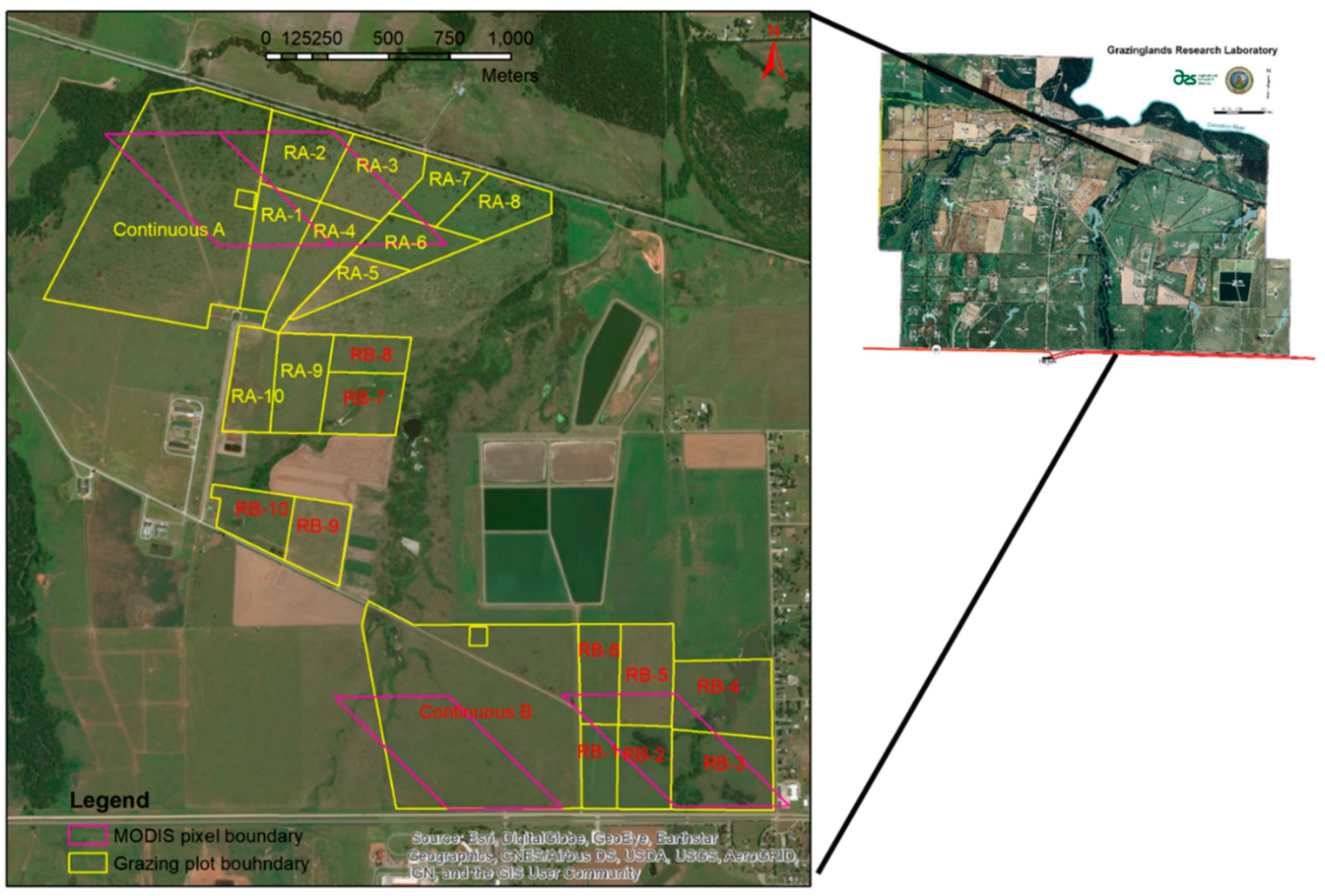
2.1. Study Area and Experiment Design
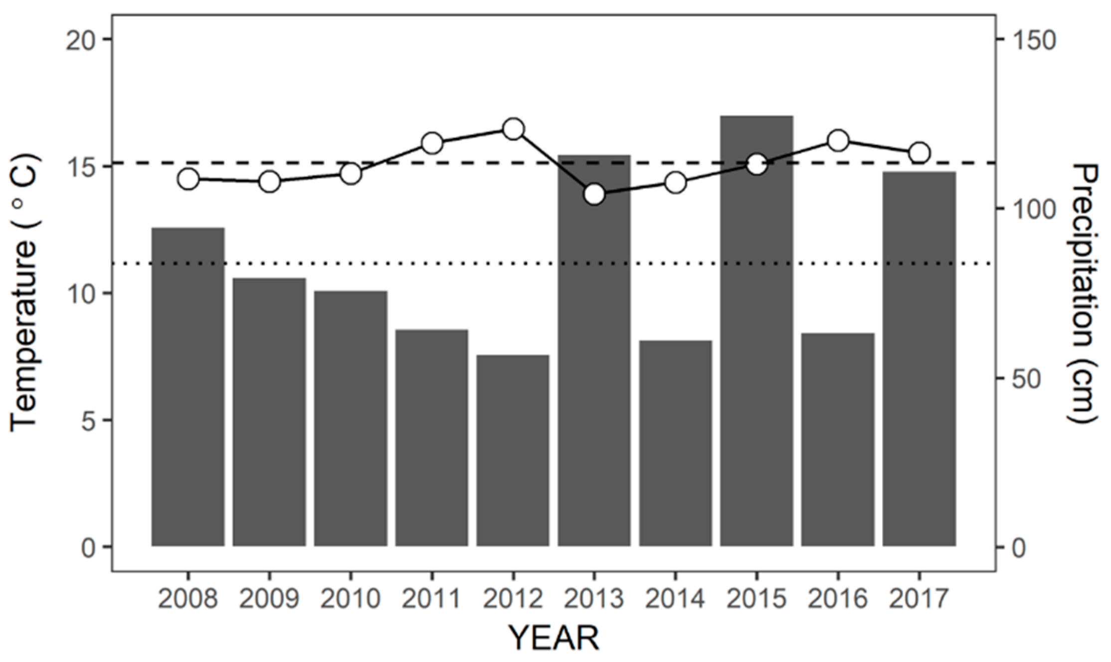
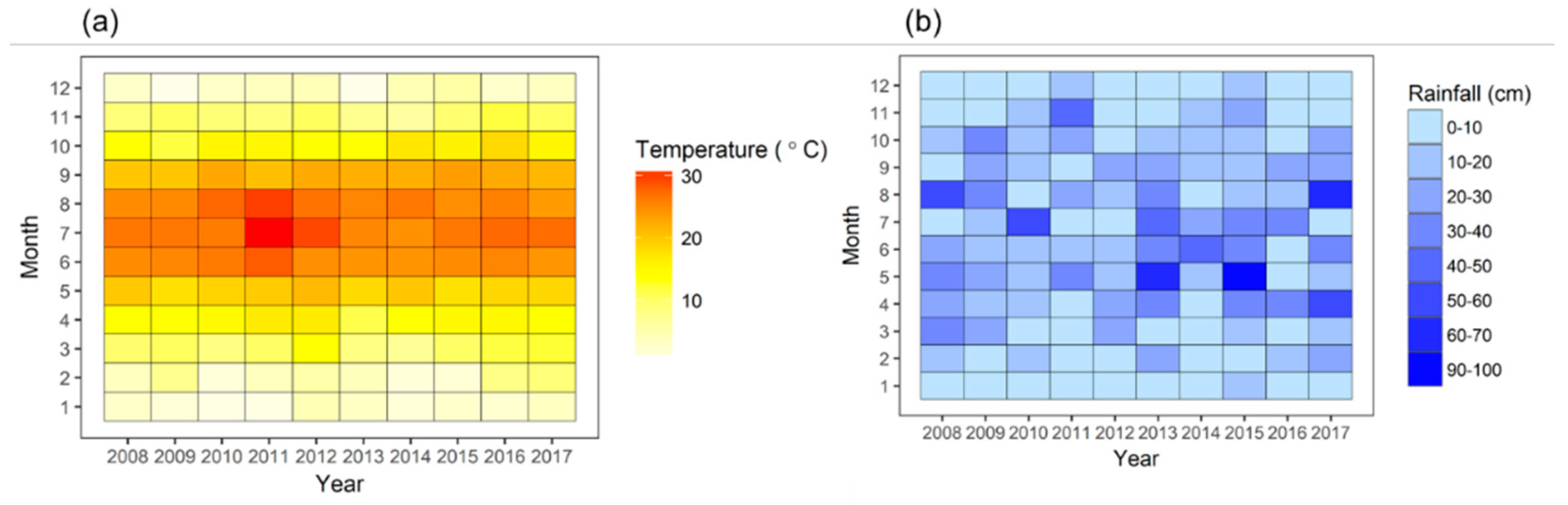
The study was conducted (Figure 1) at the United States Department of Agriculture–Agricultural Research Service (USDA–ARS), Grazinglands Research Laboratory (GRL) in El Reno, Oklahoma. It consists of two replicates (rep a and rep b) of continuous (Ca and Cb) versus rotational grazing (Ra and Rb) systems. The experiment was initiated in 2009. There were about 20 cow–calf pairs within each of the continuous grazing pastures (Ca and Cb) year-round. In comparison, around 27 cow–calf pairs were allocated in 10 paddocks of the rotational grazing systems (Ra and Rb) following the same routine each year. Cow–calf pairs in the rotational grazing systems grazed paddocks in 7 to 10 day grazing bouts depending on the vegetation conditions. The herd sizes in the continuous and rotational grazing systems were 18(±3.4) and 26(±2.5) heard year−1, respectively. The average stocking rates for Ca, Cb, and paddocks in Ra and Ra were 0.26, 0.25, 3.36, and 3.07 heard ha−1, respectively. Though the stocking rate was adjusted in continuous grazing paddocks considering pasture conditions (details about the experiment can be found in Steiner et al., 2019 in the same issue). The size of each paddock is presented in Table 1.
In the study region, the long term (1981–2010) annual average air temperature (Ta) is 15.14 °C and average annual precipitation (P) is 91.3 cm. According to data from the Soil Survey Geographic Database (https://websoilsurvey.sc.egov.usda.gov/App/HomePage.htm), multiple soil types exist in the study area (Figure S1). Most of the paddocks were typical tallgrass prairies with big bluestem (Andropogon gerardii Vitman) and Indian grass (Sorghastrum nutans Nash) as dominant species. However, there were some trees and brushy vegetation which were not edible for cattle (mainly buckbrush, Ceanothus cuneatus Nutt.), especially in Ca (Figure S2). Large proportions of Rb-4 and Rb-7 were usually covered by ponds (Figure 1).

2.2. Climate Data

The daily average Ta and total P were collected from the Oklahoma Mesonet El Reno site (35°32′54″ N, 98°2′11″ W) (http://mesonet.org/), which is located two km away from the study area. The daily Ta and P data were aggregated to monthly average Ta and sum P for 2008–2017 to show the seasonality. The annual average Ta and total P for the study period were calculated to indicate the dynamics of climate at the annual scale.

2.3. Landsat Images and the Enhanced Vegetation Index (EVI)

As Landsat 8 data (started from 2013) does not cover the whole study period (2008–2017), we also used the Landsat 7 data, which has been operating without the scan line corrector (SLC) since 2003. Fortunately, our study area is located within the central part of the image tile (Path28/Row35) and is not affected by the strips in Landsat 7 imagery caused by SLC-off. Landsat 7 and Landsat 8 surface reflectance products (Tier 2) covering the study area were downloaded from the USGS EarthExplorer (http://earthexplorer.usgs.gov) to provide an 8-day temporal resolution and 30 m spatial resolution.
False color composite images around early May and late August were used to represent the vegetation conditions in late spring and late summer of each year, depending on the data availability and its quality (Landsat 7 or Landsat 8). A commonly used vegetation index, the enhanced vegetation index (EVI) [40], was calculated using the Landsat images following the equation below (Equation (1)). EVI is linearly correlated with the green leaf area index (LAI) in crop fields [41] and it remains sensitive to canopy variations in high chlorophyll content [40]. Only clear pixels were included in analysis based on the quality assessment band.
EVI =   2.5 × ρ n i r   ρ r e d ρ n i r   +   6.0 ×   ρ r e d     7.5   ×   ρ b l u e   +   1
where ρblue, ρred, and ρnir represent surface reflectance from blue, red, and near infrared bands (841–876 nm), respectively.

2.4. Gross Primary Production (GPP) from the Vegetation Photosynthesis Model

The vegetation photosynthesis model (VPM) [42] was used to calculate the annual gross primary production (GPP) from 2008 to 2017. The VPM is a light use efficiency model which estimates GPP as a product of actual light use efficiency ( ε g ) and absorbed photosynthetically active radiation (APAR) by chlorophyll ( A P A R c h l ) .
G P P V P M =   ε g × A P A R c h l
A P A R c h l = f P A R c h l   × P A R
where f P A R c h l is set equal to EVI. The ε g is derived by down-regulating the theoretical maximum light use efficiency ( ε 0 ) with scalars of temperature (Tscalar) and water (Wscalar) stresses [42,43,44].
εg = ε0 × Tscalar × Wscalar
The VPM can be driven by either site level data [45,46,47] or remote sensing data [48]. The GPP data for the two pairs of MODIS pixels in two replicates (Figure 1) were collected from the global VPM-GPP (8-day and 500 m resolution) product [48] and the annual sums of GPP were calculated for each year.

2.5. Statistical Analysis

The statistical analysis included two parts: inter-treatment comparison (C versus R) and intra-treatment comparison (paddocks among R systems). For the inter-treatment comparison, we treated all the paddocks in the R system as a whole and compared the difference between C and R. For the intra-treatment comparison, we considered all paddocks in the R system as independent units and investigated the variations among them. The average, maximum, minimum, and standard deviation of EVI (σEVI) values were included in both inter-treatment and intra-treatment comparisons. The growing season was considered as May–September and all of the statistical values were derived for the growing season.

3. Results

3.1. Annual and Seasonal Variations of Ta and P

There were large variations in annual Ta and P during the study years (Figure 2). Compared to the long-term annual P, 2011, 2012, 2014, and 2016 were dry years, while 2013, 2015, and 2017 were wet years. Compared to the long-term annual average Ta, 2011, 2012, and 2016 were hot years, while 2013 and 2014 were cool years.
Figure 3 shows the monthly distributions of Ta and P to illustrate drought development. Summer was very hot in 2011 and 2012, especially in the month of July. In comparison, 2013 and 2015 had relatively cool summers (Figure 3a). Although the total P in 2011 was higher than in 2012, a large proportion of P (26.5%) occurred in November, a part of the non-growing season (Figure 3b), and the growing season was relatively dry and hot. Warmer spring and a good amount of P in March–April of 2012 facilitated vegetation growth in early spring. However, the peak growing months (May–August) were very dry. The dry and hot conditions made 2012 a severe summer drought year. Both 2014 and 2016 were moderate dry years, with the latter hotter than the former.

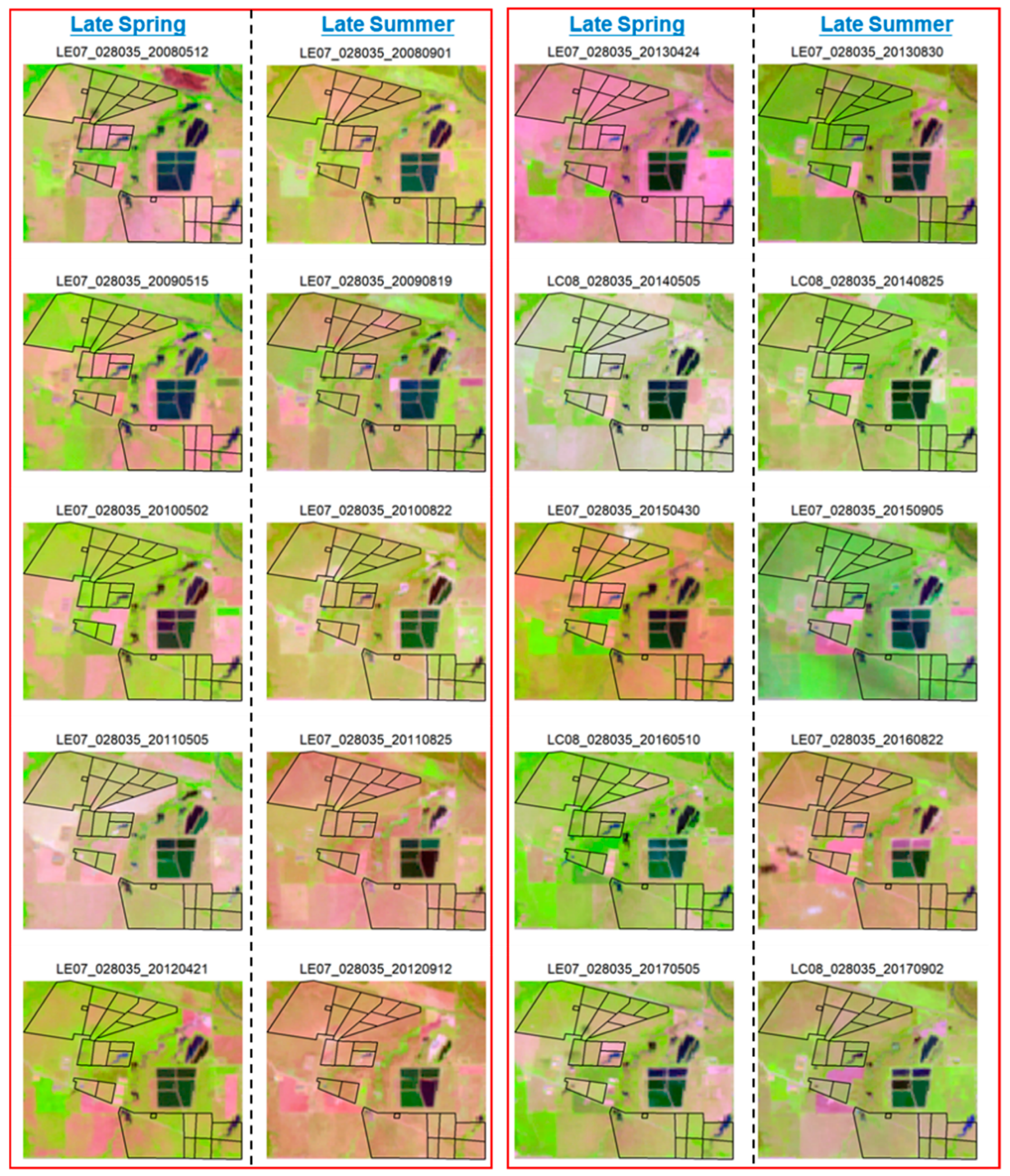
3.2. A glimpse of the Continuous and Rotational Grazing Paddocks in Late Spring and Late Summer

Figure 4 shows the false color composite images in late spring and late summer of 2008–2017. Before the experiment in 2008, the study area was heterogeneous. Ca was actually composed of two sub-paddocks. Areas that greened-up early (early May) usually entered senescence stage early (late August). Starting from 2009, most of the paddocks became synchronized in terms of greenness. The paddocks were generally green in early May and remained green until late August. However, the paddocks lost greenness relatively earlier in late August in 2011, 2012, and 2016 due to dry and hot conditions. The size of ponds in Rb-4 and Rb-7 also indicated severe droughts in 2011 and 2012 when they almost dried up.

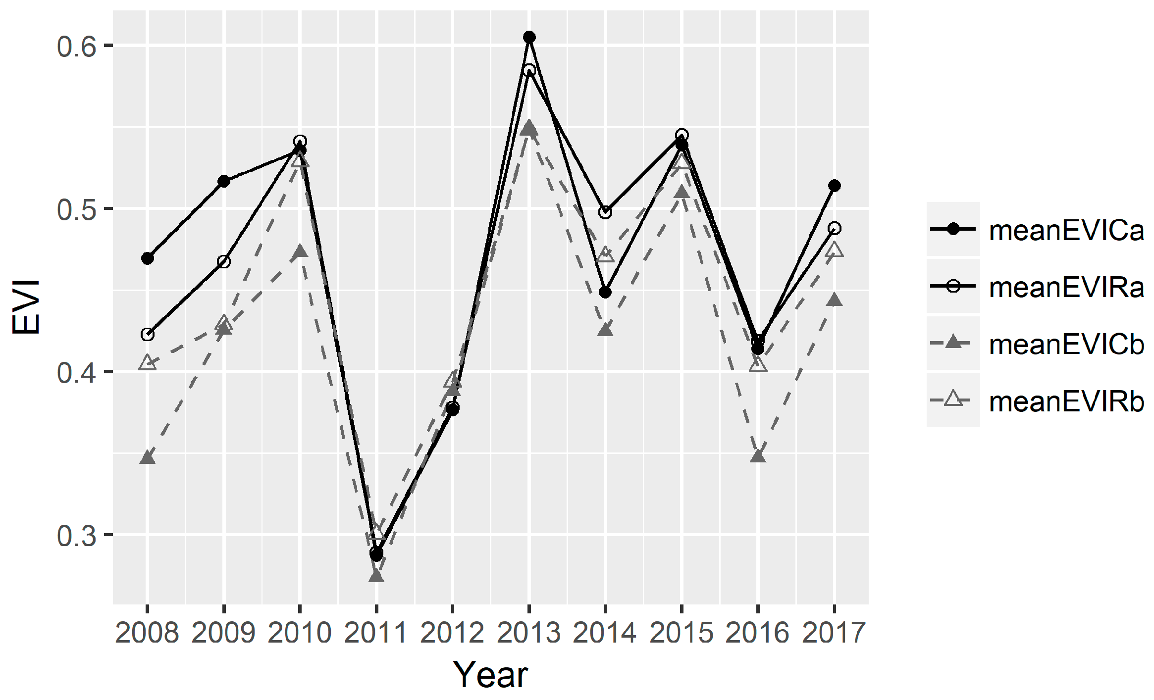
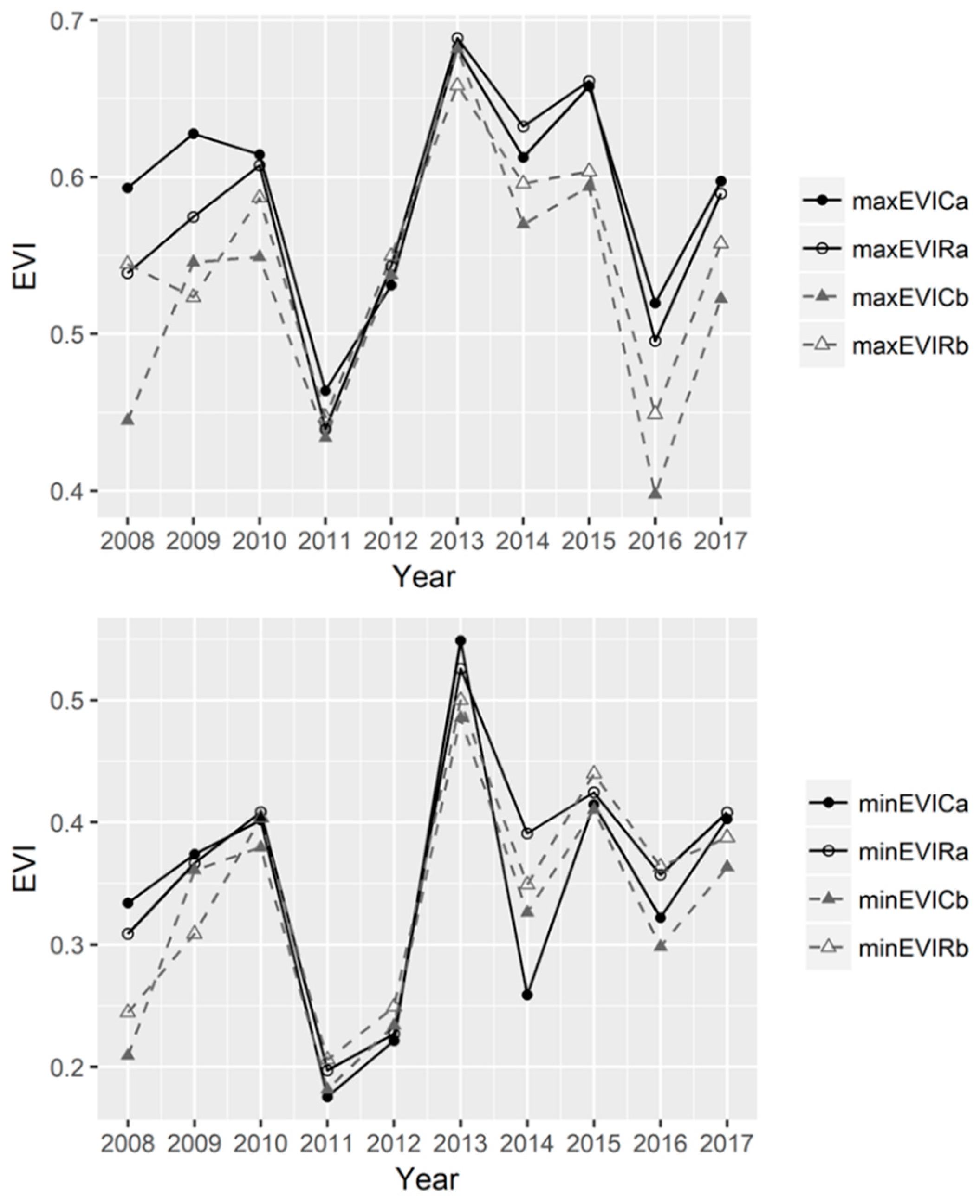
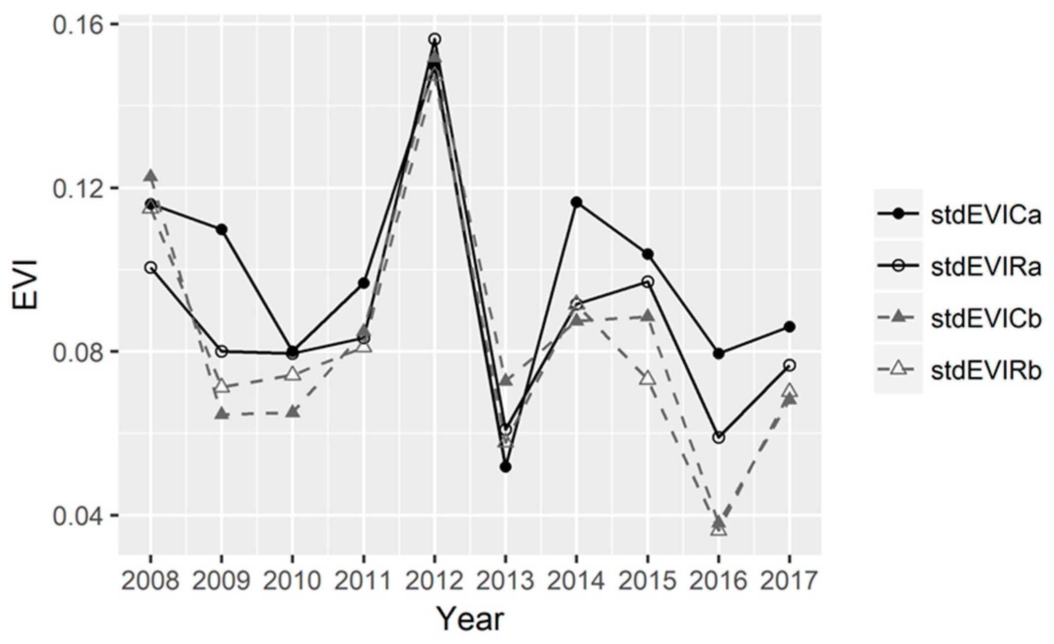
3.3. The Dynamics of EVI Values in the Continuous Versus Rotational Grazing Paddocks

The average growing season EVI is a good indicator of vegetation production during the growing season. The initial condition of average growing season EVI values (Figure 5) varied largely during the prior year (2008) and the first year of the experiment (2009). After that, climate was the major driver in affecting the average growing season EVI. The growing season average EVI values were larger than 0.5 in wet years (2013 and 2015). In severe drought years (2011 and 2012), all treatments had low average EVI values. Treatment differences were larger in moderate drought years (2014 and 2016). Even though 2012 was a drier and hotter year than 2016, the average EVI in 2012 and 2016 were comparable because of early greening up of vegetation and more growth by May in 2012 (Figure 2). The average growing season EVI in Rb was consistently larger than in Cb. However, the average growing season EVI in Ra could be similar to, higher, or lower than Ca in different years.
The maximum growing season EVI indicates the peak vegetation growth during the growing season. Rep a consistently had larger growing season maximum EVI values than rep b during the study period (Figure 6 top), indicating higher photosynthesis capability in rep a than rep b. Maximum EVIs were largest in wet years (2013 and 2015) and lowest in severe drought years (2011 and 2012), showing the significant control of climate conditions on maximum productivity in all treatments. The maximum EVI values in 2012 were higher than those in 2016 because peak EVI occurred before severe drought in 2012. The maximum EVI values only tended to converge in very wet or dry years, otherwise they had large ranges. The maximum EVI values in Rb were larger than in Cb in majority of cases. The differences in maximum EVI between Ra and Ca were smaller than between Rb and Cb.
The minimum growing season EVI can represent the low photosynthesis capability caused by climate or other stresses on vegetation. The growing season minimum EVI (Figure 6 bottom) converged more than maximum EVI, with larger differences in moderate drought years (2014 and 2016). In contrast to what it was observed in maximum EVI, the minimum EVI was much lower in 2012 than in 2016, suggesting a collapse of vegetation condition because of the severe summer drought. The minimum EVI values in both rotational grazing treatments were larger than their counterparts (Rb larger than Cb and Ra larger than Ca) in most years.
The growing season standard deviation of EVI (σEVI) shows the variation of vegetation production during the growing season. Rep a had larger growing season σEVI than rep b (Figure 7). Ca had larger σEVI than Ra in most years while the differences between Cb and Rb were small throughout the years. Ca usually had the largest σEVI because of its mixture of grass, brush, and trees, which had different seasonality.

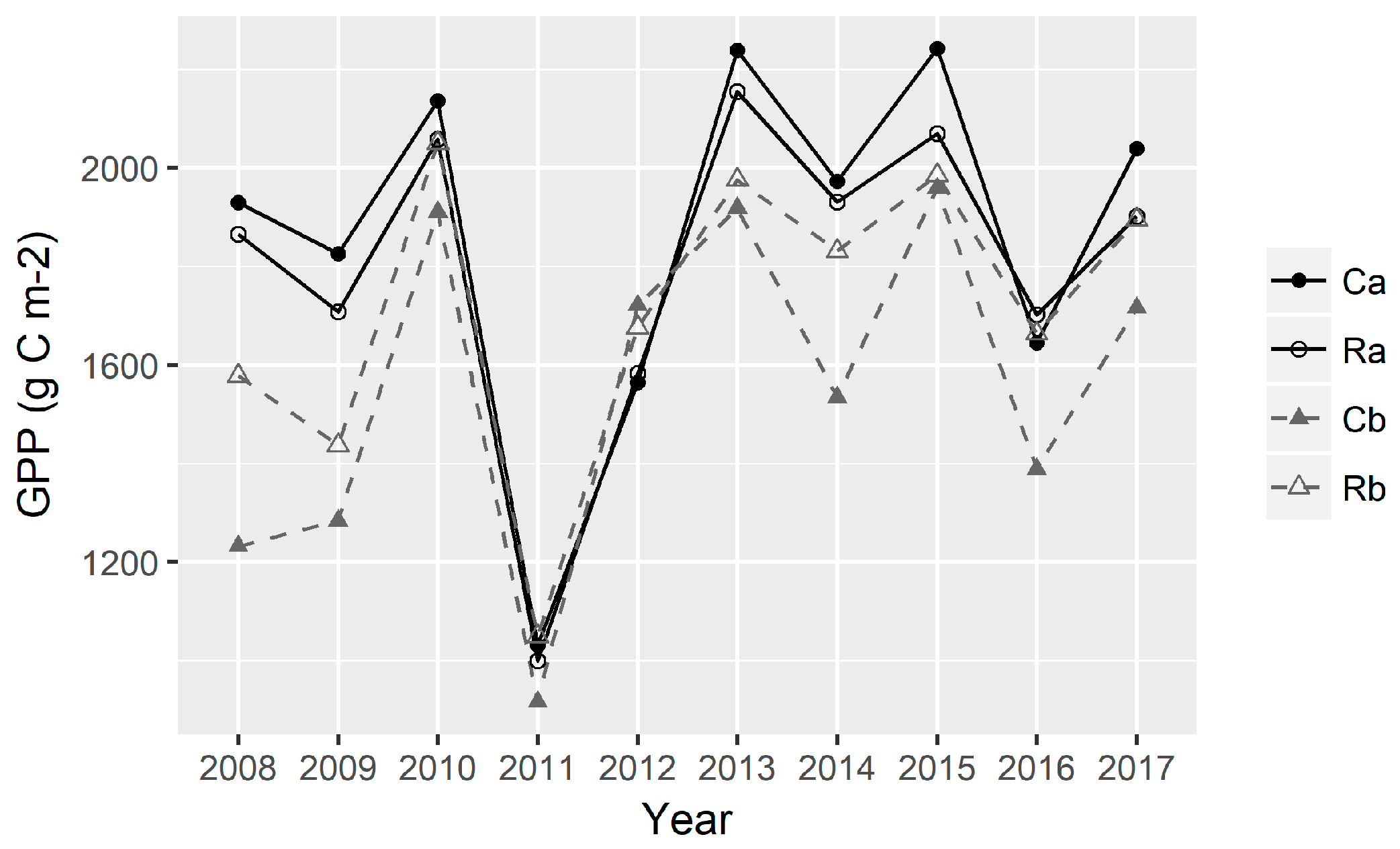
3.4. Dynamics of GPP in the Continuous Versus Rotational Grazing Paddocks

The dynamics of the annual sum of GPP (Figure 8) were similar to that of the average EVI (Figure 5) as EVI is a major input parameter in the calculation of GPP. Similar to average EVI, all treatments had the lowest GPP in 2011 due to the severe drought during the whole growing season. The GPP in 2012 and 2016 were comparable in spite of higher drought and heat stresses in the former because of early greening up of vegetation and more growth by May in 2012. The GPP in Rb was consistently larger than in Cb, especially while the GPP in Ra and Ca were similar.

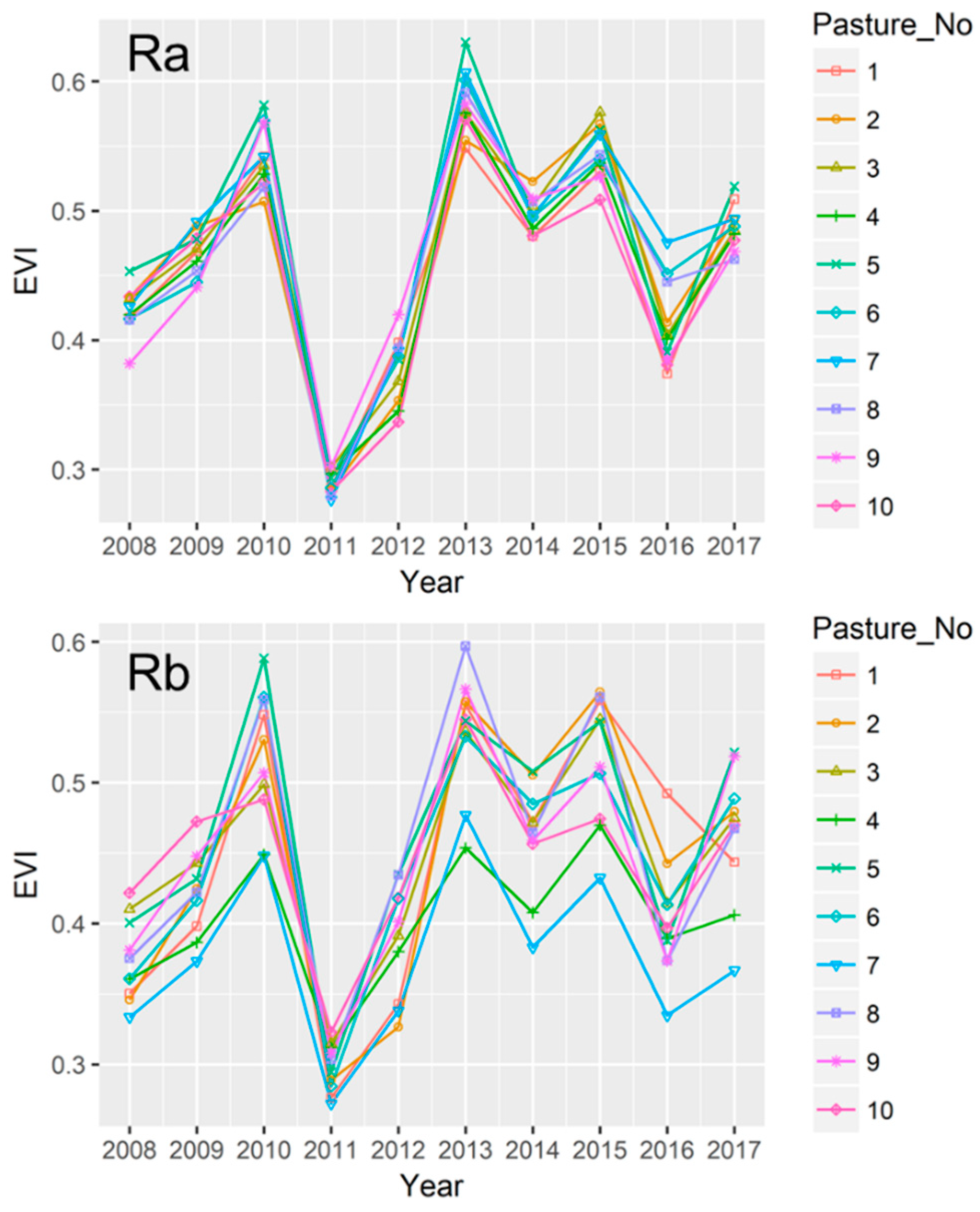
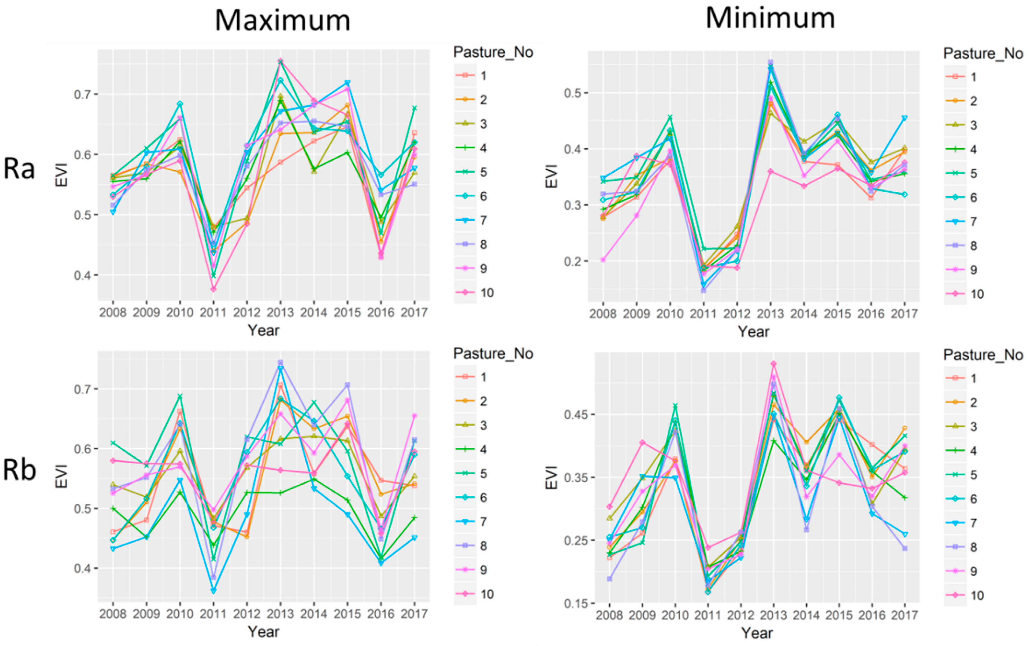
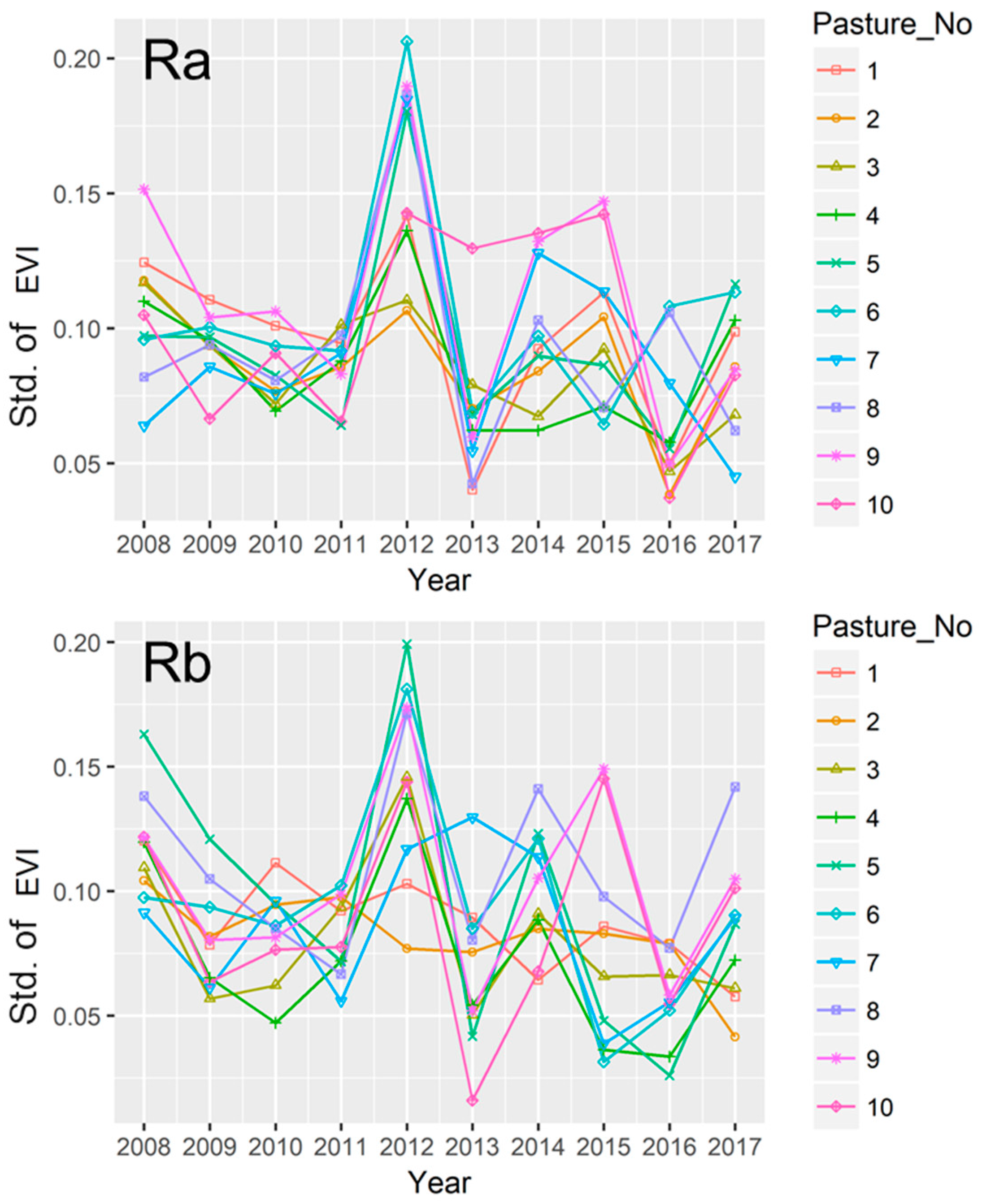
3.5. Variations in EVI among Paddocks in the Rotational Grazing Systems

Variations in EVI among paddocks in Ra and Rb were used to examine the impacts of time since grazing within an individual paddock. Overall, the variations in growing season average EVI for paddocks in both reps (Ra and Rb) were relatively small (Figure 9). Ra had lower variation in growing season average EVI than Rb, indicating the differences among pastures in rep a were smaller than in rep b. The average EVI converged only in a very dry year (2011). Rb-4 and Rb-7 usually had lower average EVI values than other paddocks because large proportions of them were covered by ponds (Figure 1) in non-drought years. The ranges of maximum EVI within a year were large and no paddocks consistently outperformed than others (Figure 10 left panels). Similarly, as found in inter-treatment comparison (Figure 6), minimum EVI among paddocks converged more than maximum EVI (Figure 10 right panels). The σEVI in Ra and Rb were the largest in 2012 (Figure 11) caused by the severe summer drought. In wet years (2013 and 2015) Ra had lower σEVI than Rb.

4. Discussion

This study provided a direct comparison of vegetation productivity in continuous and rotational grazing management systems in tallgrass prairies of the Southern Great Plains. The large climate variation during the study period allowed us to examine the differences in response to climate under continuous and rotational grazing management. Many studies indicated that multi-paddock rotational grazing can improve grassland productivity by allowing post-grazing recovery [25,32,49]. Our study found that the rotational grazing had higher vegetation production in rep b but not in rep a. Both average growing season EVI and GPP were higher in rep a than rep b probably caused by their inherent differences such as soil type. Additionally, our results indicated that productivity of tallgrass prairie was greatly controlled by climate, more specifically by the seasonality of air temperature and precipitation. This finding is also supported by other studies that compared the continuous and rotational grazing in the same experiment from perspectives of aboveground biomass (Starks et al. 2019) and landscape pattern (Ma et al. 2019), which were also presented in this issue.
The initial experiment design was to put around 25 cow–calf pairs in each of the treatments. However, the stocking rate in the continuous grazing system was adjusted according to the paddock conditions (considering woody encroachment, climate, species composition and desirable species, and grass growth). With reduced stocking rate in continuous grazing systems, the vegetation production was still similar with rotational grazing systems that had higher stocking rates. Thus, the concept of adaptive grazing management [19,21,23,50,51,52,53], adjusting grazing management depending on the vegetation and climate conditions, might be better to help ranchers to understand the necessity of adjusting their grazing routine to achieve sustainable and profitable usage of pastures.
Since little differences in vegetation growth were detected between Ca and Ra, it indirectly demonstrated that rotational grazing has higher grazing capacity, as Ca had a reduced stocking rate. Variations in EVI among paddocks in rotational grazing systems were small (Figure 11), indicating their similarity in vegetation growth. The relative small variations among paddocks in different years demonstrated that rotational grazing generated evenly distributed grazing pressure on tallgrass prairies in different climate conditions. Even with a higher stocking rate, the rotational grazing management generated similar vegetation responses with continuous grazing and an evenly grazed vegetation pattern. The results indicate the rotational grazing may support higher livestock production while maintaining sustainable usage of the tallgrass prairie pastures in the region.
The interaction of climate variability and grazing management makes the study complicated. There were very dry (2011 and 2012) and wet years (2013 and 2015) during the study period. Even the drought years had different characteristics. For example, 2011 was a growing season-long drought year and 2012 was a summer drought and hot year. The seasonal distribution of Ta and P generated different impacts on vegetation. Their dynamics combined with different grazing management controlled the grassland phenology and productivity. Thus, it is hard to conclude a general comparison between C and R for the entire study period. The average EVI only converged in very dry years (2011 and 2012) among treatments (Figure 5) and large variations exist in other years. Although 2012 was a drier and hotter year than 2016, they had comparable EVI. This difference was caused by the seasonal distribution of Ta and P. There was more precipitation in spring 2012 (March–April) than in 2016, which facilitated the vegetation growth in spring and early summer in 2012. It was hot and dry in summer 2012. Favorable vegetation growth in spring and a hot and dry summer induced a flash drought and quickly suppressed vegetation growth [45,54,55]. The largest σEVI in 2012 (Figure 7) was caused by good vegetation growth in spring and poor vegetation growth in summer. The larger average EVI in rep a than in rep b could be attributed to their original characteristics, such as soil types (Figure S1).
Besides comparing the difference between C and R, we also examined the differences among rotational grazing paddocks in both reps (Figure 9, Figure 10 and Figure 11). Except in severe drought years (2011 and 2012), large variations existed among individual paddocks in rotational grazing systems. Similar with the inter-treatment comparison, their EVI variations were mostly controlled by climate conditions. The variations in Ra were consistently smaller than in Rb, which supported the idea that the difference between rep a and rep b was caused by innate differences, such as soil type. This is also demonstrated by Ma et al. (2019) in the same issue from the shrub encroachment perspective.

5. Conclusions

Through examining the responses of vegetation to continuous and rotational grazing, this study demonstrated that vegetation growth in tallgrass prairies were mainly controlled by the seasonality of precipitation and temperature. The average EVI values only converged in a very dry year in inter- and intra-treatments comparisons. The vegetation growth was also highly related to the original pasture conditions (e.g., soil types), as rep a consistently had higher EVI values than rep b. The intra-treatment analysis showed that paddocks in rotational grazing systems had relatively small variations in different years, indicating that the rotational grazing created an even grazing pressure on grassland. The growing season average EVI and GPP were higher in Rb than in Cb. Although there were no significant differences in EVI and vegetation production between Ra and Ca, rotational grazing might increase vegetation productivity as the stocking rate in C had been reduced because of the deteriorating pasture conditions. The study suggests that an adaptive grazing management approach might better help farmers to adapt to ever-changing climatic conditions (e.g., annual and seasonal variations in air temperature and precipitation).

Supplementary Materials

The following are available online at https://www.mdpi.com/2073-4395/9/5/219/s1, Figure S1: Soil types in study area. Data is from the Soil Survey Geographic Database, Figure S2: Brush and tree in the continuous grazing pasture in rep a.

Author Contributions

Conceptualization, Y.Z. and P.H.G.; methodology, Y.Z., P.H.G., and P.W.; formal analysis Y.Z., S.M., and V.G.K.; investigation: Y.Z., S.M., and J.L.S.; data curation: J.P.S.N.; writing—original draft preparation: Y.Z., S.M., and V.G.K.; writing—review and editing: P.H.G., P.W., J.P.S.N., V.G.K., and J.L.S.; visualization: Y.Z., P.H.G., P.W., and S.M.; funding acquisition, V.G.K., P.H.G., and J.L.S.

Funding

This research was funded by USDA-NIFA’s Agriculture and Food Research Initiative (AFRI), grant number 2013-69002.

Conflicts of Interest

The authors declare no conflict of interest.

References

  1. Samson, F.B.; Knopf, F.L.; Ostlie, W.R. Great Plains ecosystems: Past, present, and future. Wildl. Soc. Bull. 2004, 32, 6–15. [Google Scholar] [CrossRef]
  2. Cunfer, G. On the Great Plains: Agriculture and Environment; Texas A&M University Press: College Station, TX, USA, 2005. [Google Scholar]
  3. Westoby, M.; Walker, B.; Noy-Meir, I. Opportunistic management for rangelands not at equilibrium. J. Range Manag. 1989, 42, 266–274. [Google Scholar] [CrossRef]
  4. Fuhlendorf, S.D.; Engle, D.M. Restoring Heterogeneity on Rangelands: Ecosystem Management Based on Evolutionary Grazing Patterns: We propose a paradigm that enhances heterogeneity instead of homogeneity to promote biological diversity and wildlife habitat on rangelands grazed by livestock. BioScience 2001, 51, 625–632. [Google Scholar]
  5. Hubbard, W.A. Rotational grazing studies in western Canada. J. Range Manag. 1951, 4, 25–29. [Google Scholar] [CrossRef]
  6. Hyder, D.N.; Sawyer, W. Rotation-deferred grazing as compared to season-long grazing on sagebrush-bunchgrass ranges in Oregon. J. Range Manag. 1951, 4, 30–34. [Google Scholar] [CrossRef]
  7. McIlvain, E.; Savage, D. Eight-year comparisons of continuous and rotational grazing on the Southern Plains Experimental Range. J. Range Manag. 1951, 4, 42–47. [Google Scholar] [CrossRef]
  8. Rogler, G.A. A twenty-five year comparison of continuous and rotation grazing in the Northern Plains. J. Range Manag. 1951, 4, 35–41. [Google Scholar] [CrossRef]
  9. Sampson, A.W. A Symposium on Rotation Grazing in North America. J. Range Manag. 1951, 4, 19–24. [Google Scholar] [CrossRef]
  10. Sampson, A.W. Range Improvement by Deferred and Rotation Grazing; Series: Bulletin of the U.S. Department of Agriculture No. 34; U.S. Department of Agriculture: Washington, DC, USA, 1913.
  11. Leo, B.M. A Variation of Deferred Rotation Grazing for Use under Southwest Range Conditions. J. Range Manag. 1954, 7, 152–154. [Google Scholar]
  12. Heady, H.F. Continuous vs. specialized grazing systems: A review and application to the California annual type. J. Range Manag. 1961, 14, 182–193. [Google Scholar] [CrossRef]
  13. Bryant, F.C.; Dahl, B.E.; Pettit, R.D.; Britton, C.M. Does short-duration grazing work in arid and semiarid regions? J. Soil Water Conserv. 1989, 44, 290–296. [Google Scholar]
  14. White, M.R.; Pieper, R.D.; Donart, G.B.; Trifaro, L.W. Vegetational response to short-duration and continuous grazing in southcentral New Mexico. J. Range Manag. 1991, 44, 399–403. [Google Scholar] [CrossRef]
  15. Gillen, R.L.; Gillen, R.L.; McCollum III, F.T.; Tate, K.W.; Hodges, M.E. Tallgrass prairie response to grazing system and stocking rate. J. Range Manag. 1998, 51, 139–146. [Google Scholar] [CrossRef]
  16. Jacobo, E.J.; Rodríguez, A.M.; Bartoloni, N.; Deregibus, V.A. Rotational Grazing Effects on Rangeland Vegetation at a Farm Scale. Rangel. Ecol. Manag. 2006, 59, 249–257. [Google Scholar] [CrossRef]
  17. Briske, D.D.; Derner, J.D.; Brown, J.R.; Fuhlendorf, S.D.; Teague, W.R.; Havstad, K.M.; Gillen, R.L.; Ash, A.J.; Willms, W.D. Benefits of rotational grazing on rangelands: An evaluation of the experimental evidence. Rangel. Ecol. Manag. 2008, 61, 3–17. [Google Scholar] [CrossRef]
  18. Briske, D.D.; Derner, J.D.; Brown, J.R.; Fuhlendorf, S.D.; Teague, W.R.; Havstad, K.M.; Gillen, R.L.; Ash, A.J.; Willms, W.D. Rotational Grazing on Rangelands: Reconciliation of Perception and Experimental Evidence. Rangel. Ecol. Manag. 2008, 61, 3–17. [Google Scholar] [CrossRef]
  19. Budd, B.; Thorpe, J. Benefits of Managed Grazing: A Manager’s Perspective. Rangelands 2009, 31, 11–14. [Google Scholar] [CrossRef]
  20. Briske, D.D.; Sayre, N.F.; Huntsinger, L.; Fernández-Giménez, M.; Budd, B.; Derner, J.D. Origin, Persistence, and Resolution of the Rotational Grazing Debate: Integrating Human Dimensions into Rangeland Research. Rangel. Ecol. Manag. 2011, 64, 325–334. [Google Scholar] [CrossRef]
  21. Teague, R.; Provenza, F.; Kreuter, U.; Steffens, T.; Barnes, M. Multi-paddock grazing on rangelands: Why the perceptual dichotomy between research results and rancher experience? J. Environ. Manag. 2013, 128, 699–717. [Google Scholar] [CrossRef] [PubMed]
  22. Wang, T.; Teague, W.R.; Park, S.C. Evaluation of Continuous and Multipaddock Grazing on Vegetation and Livestock Performance—A Modeling Approach. Rangel. Ecol. Manag. 2016, 69, 457–464. [Google Scholar] [CrossRef]
  23. Becker, W.; Kreuter, U.; Atkinson, S.; Teague, R. Whole-Ranch Unit Analysis of Multipaddock Grazing on Rangeland Sustainability in North Central Texas. Rangel. Ecol. Manag. 2017, 70, 448–455. [Google Scholar] [CrossRef]
  24. Norton, B.E.; Barnes, M.; Teague, R. Grazing Management Can Improve Livestock Distribution. Rangelands 2013, 35, 45–51. [Google Scholar] [CrossRef]
  25. Teague, W.; Dowhower, S.L.; Baker, S.A.; Haile, N.; DeLaune, P.B.; Conover, D.M. Grazing management impacts on vegetation, soil biota and soil chemical, physical and hydrological properties in tall grass prairie. Agric. Ecosyst. Environ. 2011, 141, 310–322. [Google Scholar] [CrossRef]
  26. Heitschmidt, R.; Dowhower, S.; Walker, J. Some effects of a rotational grazing treatment on quantity and quality of available forage and amount of ground litter. J. Range Manag. 1987, 40, 318–321. [Google Scholar] [CrossRef]
  27. Hart, R.H.; Samuel, M.J.; Test, P.S.; Smith, M.A. Cattle, vegetation, and economic responses to grazing systems and grazing pressure. J. Range Manag. 1988, 41, 282–286. [Google Scholar] [CrossRef]
  28. Hickman, K.R.; Hartnett, D.C.; Cochran, R.C.; Owensby, C.E. Grazing management effects on plant species diversity in tallgrass prairie. Rangel. Ecol. Manag. 2004, 57, 58–66. [Google Scholar] [CrossRef]
  29. Wood, M.K.; Blackburn, W.H. Vegetation and soil responses to cattle grazing systems in the Texas Rolling Plains. J. Range Manag. 1984, 37, 303–308. [Google Scholar] [CrossRef]
  30. Derner, J.D.; Hart, R.H. Grazing-induced modifications to peak standing crop in northern mixed-grass prairie. Rangel. Ecol. Manag. 2007, 60, 270–276. [Google Scholar]
  31. Derner, J.D.; Hart, R.H. Livestock and vegetation responses to rotational grazing in short-grass steppe. West. North Am. Nat. 2007, 67, 359–367. [Google Scholar] [CrossRef]
  32. Cassels, D.M.; Gillen, R.L.; Ted McCollum, F.; Tate, K.W.; Hodges, M.E. Effects of grazing management on standing crop dynamics in tallgrass prairie. J. Range Manag. 1995, 48, 81–84. [Google Scholar] [CrossRef]
  33. Martin, S.C.; Ward, D.E. Perennial grasses respond inconsistently to alternate year seasonal rest. Rangel. Ecol. Manag. J. Range Manag. Arch. 1976, 29, 346. [Google Scholar] [CrossRef]
  34. Reardon, P.O.; Merrill, L.B. Vegetative response under various grazing management systems in the Edwards Plateau of Texas. J. Range Manag. 1976, 29, 195–198. [Google Scholar] [CrossRef]
  35. Kawamura, K.; Akiyama, T.; Yokota, H.O.; Tsutsumi, M.; Yasuda, T.; Watanabe, O.; Wang, S. Quantifying grazing intensities using geographic information systems and satellite remote sensing in the Xilingol steppe region, Inner Mongolia, China. Agric. Ecosyst. Environ. 2005, 107, 83–93. [Google Scholar] [CrossRef]
  36. Numata, I.; Roberts, D.A.; Chadwick, O.A.; Schimel, J.; Sampaio, F.R.; Leonidas, F.C.; Soares, J.V. Characterization of pasture biophysical properties and the impact of grazing intensity using remotely sensed data. Remote Sens. Environ. 2007, 109, 314–327. [Google Scholar] [CrossRef]
  37. Ma, S.; Zhou, Y.; Gowda, P.; Chen, L.; Steiner, J.; Starks, P.; Neel, J. Evaluating the impacts of continuous and rotational grazing on tallgrass prairie landscape using high spatial resolution imagery. Agronomy 2019, in press. [Google Scholar]
  38. Starks, P.J.; Steiner, J.L.; Neel, J.P.S.; Turner, K.E.; Northup, B.K.; Brown, M.A.; Gowda, P.H. Assessment of the SPEI as a potential management tool for grasslands. Agronomy 2019, in press. [Google Scholar]
  39. Steiner, J.L.; Starks, P.J.; Neel, J.P.S.; Northup, B.K.; Gowda, P.H.; Brown, M.A.; Coleman, S. Managing Tallgrass Prairies for Productivity and Ecological Function: A Long Term Grazing Experiment in the Southern Great Plains, USA. Agronomy 2019, in press. [Google Scholar]
  40. Huete, A.; Didan, K.; Miura, T.; Rodriguez, E.P.; Gao, X.; Ferreira, L.G. Overview of the radiometric and biophysical performance of the MODIS vegetation indices. Remote Sens. Environ. 2002, 83, 195–213. [Google Scholar] [CrossRef]
  41. Boegh, E.; Søgaard, H.; Broge, N.; Hasager, C.B.; Jensen, N.O.; Schelde, K.; Thomsen, A. Airborne multispectral data for quantifying leaf area index, nitrogen concentration, and photosynthetic efficiency in agriculture. Remote Sens. Environ. 2002, 81, 179–193. [Google Scholar] [CrossRef]
  42. Xiao, X.; Hollinger, D.; Aber, J.; Goltz, M.; Davidson, E.A.; Zhang, Q.; Moore III, B. Satellite-based modeling of gross primary production in an evergreen needleleaf forest. Remote Sens. Environ. 2004, 89, 519–534. [Google Scholar] [CrossRef]
  43. Xiao, X.; Zhang, Q.; Braswell, B.; Urbanski, S.; Boles, S.; Wofsy, S.; Moore III, B.; Ojima, D. Modeling gross primary production of temperate deciduous broadleaf forest using satellite images and climate data. Remote Sens. Environ. 2004, 91, 256–270. [Google Scholar] [CrossRef]
  44. Wagle, P.; Xiao, X.; Torn, M.S.; Cook, D.R.; Matamala, R.; Fischer, M.L.; Jin, C.; Dong, J.; Biradar, C. Sensitivity of vegetation indices and gross primary production of tallgrass prairie to severe drought. Remote Sens. Environ. 2014, 152, 1–14. [Google Scholar] [CrossRef]
  45. Zhou, Y.; Xiao, X.; Wagle, P.; Bajgain, R.; Mahan, H.; Basara, J.B.; Dong, J.; Qin, Y.; Zhang, G.; Luo, Y. Examining the short-term impacts of diverse management practices on plant phenology and carbon fluxes of Old World bluestems pasture. Agric. For. Meteorol. 2017, 237–238, 60–70. [Google Scholar] [CrossRef]
  46. Bajgain, R.; Xiao, X.; Basara, J.; Wagle, P.; Zhou, Y.; Mahan, H.; Gowda, P.; McCarthy, H.R.; Northup, B.; Neel, L.; et al. Carbon dioxide and water vapor fluxes in winter wheat and tallgrass prairie in central Oklahoma. Sci. Total Environ. 2018, 644, 1511–1524. [Google Scholar] [CrossRef]
  47. Doughty, R.; Xiao, X.; Wu, X.; Zhang, Y.; Bajgain, R.; Zhou, Y.; Qin, Y.; Zou, Z.; McCarthy, H.R.; Friedman, J.; et al. Responses of gross primary production of grasslands and croplands under drought, pluvial, and irrigation conditions during 2010–2016, Oklahoma, USA. Agric. Water Manag. 2018, 204, 47–59. [Google Scholar] [CrossRef]
  48. Zhang, Y.; Xiao, X.; Wu, X.; Zhou, S.; Zhang, G.; Qin, Y.; Dong, J. A global moderate resolution dataset of gross primary production of vegetation for 2000–2016. Sci. Data 2017, 4, 170165. [Google Scholar] [CrossRef]
  49. Teague, W.; Dowhower, S.; Waggoner, J. Drought and grazing patch dynamics under different grazing management. J. Arid Environ. 2004, 58, 97–117. [Google Scholar] [CrossRef]
  50. Díaz-Solís, H.; Grant, W.E.; Kothmann, M.M.; Teague, W.R.; Díaz-García, J.A. Adaptive management of stocking rates to reduce effects of drought on cow–calf production systems in semi-arid rangelands. Agric. Syst. 2009, 100, 43–50. [Google Scholar] [CrossRef]
  51. Teague, W.R.; Provenza, F.; Norton, B.; Steffens, T.; Barnes, M.; Kothmann, M.; Roath, R. Benefits of multi-paddock grazing management on rangelands: Limitations of experimental grazing research and knowledge gaps. In Grasslands: Ecology, Management and Restoration; Schröder, H., Ed.; Nova Science Publishers: Hauppauge, NY, USA, 2009; pp. 41–80. [Google Scholar]
  52. Torell, L.A.; Murugan, S.; Ramirez, O.A. Economics of Flexible Versus Conservative Stocking Strategies to Manage Climate Variability Risk. Rangel. Ecol. Manag. 2010, 63, 415–425. [Google Scholar] [CrossRef]
  53. Roche, L.M.; Cutts, B.B.; Derner, J.D.; Lubell, M.N.; Tate, K.W. On-Ranch Grazing Strategies: Context for the Rotational Grazing Dilemma. Rangel. Ecol. Manag. 2015, 68, 248–256. [Google Scholar] [CrossRef]
  54. Otkin, J.A.; Anderson, M.C.; Hain, C.; Svoboda, M.; Johnson, D.; Mueller, R.; Tadesse, T.; Wardlow, B.; Brown, J. Assessing the evolution of soil moisture and vegetation conditions during the 2012 United States flash drought. Agric. For. Meteorol. 2016, 218, 230–242. [Google Scholar] [CrossRef] [Green Version]
  55. Zhou, Y.; Xiao, X.; Zhang, G.; Wagle, P.; Bajgain, R.; Dong, J.; Basara, J.; Jin, C.; Anderson, M.C.; Hain, C.; et al. Quantifying agricultural drought in tallgrass prairie region in the U.S. Southern Great Plains through analysis of a water-related vegetation index from MODIS images. Agric. For. Meteorol. 2017, 246 (Suppl. C), 111–122. [Google Scholar] [CrossRef]
Figure 1. Location of the study area overlapping with MODIS pixels. The right-hand panel shows the location of the study area within the United States Department of Agriculture-Agricultural Research Service (USDA-ARS), Grazinglands Research Laboratory (GRL).
Agronomy 09 00219 g001
Figure 2. Annual average air temperature (line with open circles) and total precipitation (vertical bars). Long dash line indicates long term annual average temperature while dot line is for long term annual total precipitation.
Agronomy 09 00219 g002
Figure 3. Seasonal distributions of air temperature (a) and precipitation (b).
Agronomy 09 00219 g003
Figure 4. False color composite images (shortwave infrared (SWIR-2), near infrared (NIR), and red bands as RGB) for continuous and rotational grazing paddocks around early May and late August. Green color represents green vegetation and pink or brown color represent dry grasses or soil. The title of each panel includes three parts separated by an underscore: the sensor (LE07 for Landsat 7 ETM+ and LC08 for Landsat 8 OLI/TIRS combined), the path/row number, and acquisition date of the image.
Agronomy 09 00219 g004
Figure 5. Growing season average EVI from Landsat 7 for different treatments in rep a and rep b. Solid lines are for rep a and dashed lines are for rep b. Solid and hollow shapes represent continuous grazing and rotational grazing.
Agronomy 09 00219 g005
Figure 6. Growing season maximum and minimum EVI from Landsat 7 for different treatments.
Agronomy 09 00219 g006
Figure 7. Growing season standard deviation of EVI from Landsat 7 for different treatments.
Agronomy 09 00219 g007
Figure 8. Annual sum of GPP in different treatments.
Agronomy 09 00219 g008
Figure 9. Growing season average EVI from Landsat 7 for paddocks in rotational grazing.
Agronomy 09 00219 g009
Figure 10. Growing season maximum and minimum EVI from Landsat 7 for paddocks in rotational grazing.
Agronomy 09 00219 g010
Figure 11. Growing season standard deviation EVI from Landsat 7 for paddocks in rotational grazing.
Agronomy 09 00219 g011
Table 1. The size of paddocks in the grazing experiment: replications a and b of continuous (Ca and Cb) and rotational (Ra and Rb) grazing.
Plot NameArea (ha)Plot NameArea (ha)
Ca58.6Cb62.7
Ra-19.3Rb-15.1
Ra-29.2Rb-27.5
Ra-39.5Rb-312.9
Ra-49.2Rb-412.2
Ra-54.4Rb-59.0
Ra-66.7Rb-66.7
Ra-77.6Rb-79.1
Ra-85.9Rb-86.6
Ra-98.7Rb-97.0
Ra-107.6Rb-106.7

