Evaluating the Impacts of Continuous and Rotational Grazing on Tallgrass Prairie Landscape Using High-Spatial-Resolution Imagery

Abstract

This study evaluated the impacts of different grazing treatments (continuous (C) and rotational (R) grazing) on tallgrass prairie landscape, using high-spatial-resolution aerial imagery (1-m at RGB and near-infrared bands) of experimental C and R pastures within two replicates (Rep A and Rep B) in the southern Great Plains (SGP) of the United States. The imagery was acquired by the National Agriculture Imagery Program (NAIP) during the agricultural growing season of selected years (2010, 2013, 2015, and 2017) in the continental United States. Land cover maps were generated by combining visual interpolation, a support vector machine, and a decision tree classifier. Landscape metrics (class area, patch number, percentage of landscape, and fragmentation indices) were calculated from the FRAGSTATS (a computer software program designed to compute a wide variety of landscape metrics for categorical map patterns) based on land cover results. Both the metrics and land cover results were used to analyze landscape dynamics in the experiment pastures. Results showed that both grass and shrubs of different pastures differed largely in the same year and had significant annual dynamics controlled by climate. High stocking intensity delayed grass growth. A large proportion of bare soil occurred in sub-paddocks of rotational grazing that were just grazed or under grazing. Rep A experienced rapid shrub encroachment, with a large proportion of shrub at the beginning of the experiment. Shrub may occupy 41% of C and 15% of R in Rep A by 2030, as revealed by the linear regression analysis of shrub encroachment. In contrast, shrub encroachment was not significant in Rep B, which only had a small number of shrub patches at the beginning of the experiment. This result indicates that the shrub encroachment is mainly controlled by the initial status of the pastures instead of grazing management. However, the low temporal resolution of the NAIP imagery (one snapshot in two or three years) limits our comparison of the continuous and rotational grazing at the annual scale. Future studies need to combine NAIP imagery with other higher temporal resolution imagery (e.g., WorldView), in order to better evaluate the interannual variabilities of grass productivity and shrub encroachment.

1. Introduction

Tallgrass prairie provides various ecological (e.g., carbon sequestration and biodiversity) and economic (e.g., forage) benefits for people in the Great Plains of the United States. However, the distribution and condition of the tallgrass prairie is threatened by agricultural land use (e.g., conversion to crops) and land management (e.g., different grazing management systems). The tallgrass prairie provides nutritious forage for cattle grazing [1] in the Great Plains, which is a major revenue stream for farmers in the region [2]. Cattle grazing is an important human disturbance to the tallgrass prairie landscape patterns (e.g., reducing landscape heterogeneity) and can affect its ecosystem productivity and health [3,4]. Continuous grazing with a moderate stocking rate (around six acres per animal unit for a tallgrass prairie, with an average production of 2,885 kg per acre in the region [5]) and rotational grazing with a relatively high stocking rate are two main grazing management systems nowadays. Rotational grazing has been recommended since the mid-20th century, as an effective way to maintain pasture productivity and sustainability [6,7,8,9,10]. Theoretically, multi-paddock rotational grazing has high stocking in each paddock, which may lead to more even spatial distribution of livestock grazing [11] and reduce bush encroachment [12]. Rotational grazing also allows for the rest of paddocks during different periods of the year, which may help improve landscape diversity or productivity [13,14,15]. In continuously grazed pastures, cattle may preferentially graze specific locations the majority of the time, which can cause landscape fragmentation and uneven grass coverage. However, there is still debate on whether rotational grazing clearly outperforms continuous grazing or not in terms of plant or livestock productivity [13,15,16,17,18,19,20,21,22,23,24,25,26,27].

As a landscape dominated by grasses, the grass coverage of pastures is an important indicator of grassland landscape and productivity in tallgrass prairie. The presence of shrubs in the tallgrass prairie as a result of invasion is becoming an important component in many of tallgrass prairie ecosystems. Woody shrub invasion in the Great Plains [28,29] can cause a decrease in species richness and diminish cattle grazing capacity [12]. Many researchers have found that shrub invasion may be mitigated by grazing [12,30]. Thus, investigating the impacts of grazing management on grass condition and shrub invasion is of great importance.

Since different grazing management systems could exert different impacts on tallgrass prairie landscape patterns. Evaluating the impacts and further identifying an efficient and sustainable grazing management system for the tallgrass pastures is essential to maintain the health of prairie ecosystem [31,32,33]. However, evaluation of the impacts of grazing on tallgrass prairie landscape is challenging, mostly due to the potential mismatch between pasture size and spatial resolution of free and commonly used satellite datasets (e.g., MODIS and Landsat, with spatial resolutions of 500 m and 30 m, respectively). The National Agriculture Imagery Program (NAIP) acquires high spatial resolution (1 m) multi-spectral (red, green, blue, and near-infrared) aerial imagery during the agricultural growing season in the continental United States [34]. The high spatial resolution of NAIP imagery provides us an opportunity to study landscape dynamics within paddocks not of sufficient size to be studied using medium- to low-spatial-resolution data sets.

To compare and contrast differences in continuously and rotationally grazed pastures with regard to variations in grass condition and woody shrub, experimental pastures composed of two treatments (continuous grazing (C) versus rotational grazing (R)), with two repetitions for each treatment (Rep A and Rep B) located in El Reno, Oklahoma, United States were used in this study. This study evaluated the impacts of different grazing treatments (continuous versus rotational grazing) on tallgrass prairie landscape, using NAIP imagery of the experimental pastures. Visual interpretation and two supervised classification methods were combined to get accurate classification results. Landscape metrics are used to quantitatively analyze the response of landscape patterns to continuous and rotational grazing. The findings of this study can help develop better grazing management systems for forage production and shrub encroachment control.

2. Materials and Methods

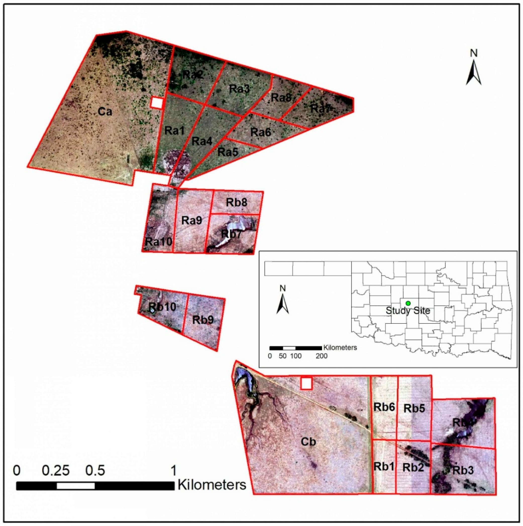
2.1. Study Area and Experiment Design

The study area is located at the United States Department of Agriculture Agricultural Research Service (USDA-ARS) Grazinglands Research Laboratory (GRL) in El Reno, OK, United States. The study area is typical tallgrass prairie in the Southern Great Plain (SGP). The main grass species in the study area are big bluestem (Andropogon gerardii Vitman), little bluestem (Schizachyrium scoparium (Michs.) Nash), indiangrass (Sorghastrum nutans (L.) Nash), and switchgrass (Panicum virgatum L.). The main woody shrub in the area is buckbrush (Symphoricarpos orbiculatus Moench), and is not edible by cattle. Photos of main grass and shrub species were shown in Figure S1. Long term annual average air temperature is 15.14 °C, and total precipitation is 91.3 cm. Dominant soils consist mainly of Norge silt loams (Fine–silty, mixed, active thermic Udic Paleustolls), Renfrow (fine, mixed super-active, thermic Udertic Paleustolls), and Kirkland silt loams (Fine–silty, mixed super-active, thermic Cumulic Hapulstolls) [35].

The study was comprised of two grazing treatments (continuous (C) and rotational (R)), with two replicates (Rep A and Rep B) for each treatment (Figure 1). The areas of the pastures were 58.6, 62.7, 78.6, and 82.7 ha for C in Rep A (Ca), C in Rep B (Cb), R in Rep A (Ra), and R in Rep B (Rb), respectively. The R pastures were further sub-divided into 10 approximately equally-sized cells. Grazing in Ca and Ra began in 2009, while Cb and Rb started grazing in 2011. The number of grazing cattle varied across years: 10 to 20 cow–calf pairs in the C treatments, and 20 to 27 cow–calf pairs in the R treatments. Cattle herds stayed in the C treatments year-round, while they rotated within the 10 cells in 7- to 10-day grazing bouts, depending on the vegetation conditions. More detail on the grazing experiment can be found in Steiner et al. [36].

2.2. National Agriculture Imagery Program Imagery and the Normalized Difference Vegetation Index

The NAIP acquires multi-spectral aerial imagery (natural color (red, green, and blue, or RGB) and near-infrared (NIR)) during the agricultural growing seasons. NAIP imagery is acquired at a one-meter ground sample distance, with a horizontal accuracy that matches within six meters of photo-identifiable ground control points that are used during image inspection. Every NAIP imagery has no more than 10% cloud cover, weather conditions permitting. Horizontal accuracy and tonal quality are inspected for all imagery. Thus, these images are analysis-ready. We downloaded the four-band (RGB and NIR) NAIP product of the experimental pastures for 5 May 2010, 2 June 2013, 6 June 2015, and 21 May 2017 using the Google Earth Engine. The Normalized Difference Vegetation Index (NDVI) was calculated from the red and near-infrared bands (Equation 1) [37], and the index was then used to estimate grass coverage.

$$NDVI=\frac{{\rho }_{nir}-{\rho }_{red}}{{\rho }_{nir}+{\rho }_{red}}$$

(1)

where ρ_red, and ρ_nir represent surface reflectance from red and near infrared band (841–876 nm), respectively.

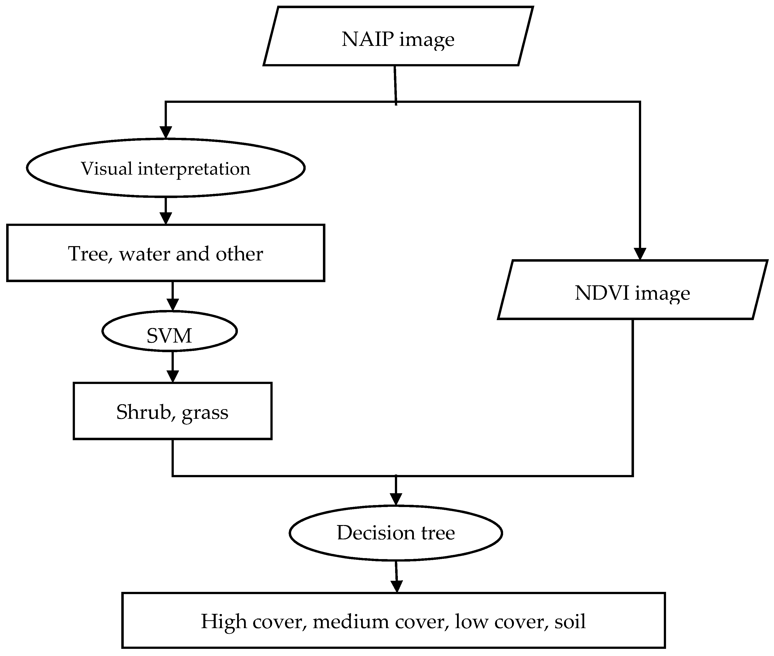
2.3. Image Classification

According to our field survey of land cover types, the main land cover classes in the study area are grass, shrub, tree, water body, and miscellaneous (e.g., paths and shades for cattle). The grass category can be further subdivided into four levels of coverage: high, medium, low cover, and bare soil. Bare soil is temporary in paddocks, especially in R pastures that are currently under grazing. Therefore, it is also included in the grass category. In order to achieve a high classification accuracy, we combined visual interpretation and two supervised classification methods (support vector machine (SVM) and a decision tree classifier). The work flow is shown in Figure 2.

2.3.1. Visual Interpretation

Visual interpretation is commonly used, when good prior knowledge of the study area exists, and one or more cover types are easily distinguished based on color, size, shape, and tonal qualities, especially for high spatial aerial imagery. In this study, trees, man-made features, and water bodies were easily identified, and were manually classified by this method. As trees occupied a small area and distributed in a fixed location, with different sizes in different years depending on growth conditions, it is easier to extract them by interpretation.

2.3.2. Support Vector Machine

Although shrub and grass have some overlapping spectral features, they have different visual textural features. We initially evaluated the performances of the support vector machine (SVM), maximum likelihood (ML), and artificial neural network (ANN) in identifying shrub and the various levels of grass cover after the manually-identified tree, water body, and man-made feature classes were masked from the images. Before the classification, a training dataset and validation dataset representative of shrub and grass were acquired by combining a field survey, Google Earth images, and the region of interest (ROI) tool of NAIP imagery. The initial analysis revealed that the SVM achieves a higher level of classification accuracy than the other two methods (

Table 1. Accuracy assessment of the support vector machine (SVM), maximum likelihood (ML), and artificial neural network (ANN).

Classifier	Overall Accuracy(%)	Kappa Coefficient
SVM	93.58	0.87
ANN	92.6	0.85
ML	87.15	0.75

); thus, SVM was adopted in classification throughout the study years.

The SVM classifier is based on statistical learning theory and was initially designed for two-class problems [38,39]. The SVM has been widely reported as an outstanding supervised classification method. With given training datasets, SVM outputs an optimal hyperplane that separates categorizes. Kernel function selection and its parameter (gamma, pyramid levels, etc.) determinations affect SVM classifier performance. SVM classification in this study was executed in radial basis function kernel types by using the default value. The default parameter value of gamma is 0.25, the penalty parameter is 100, the pyramid level is 0, and the classification probability threshold is 0.

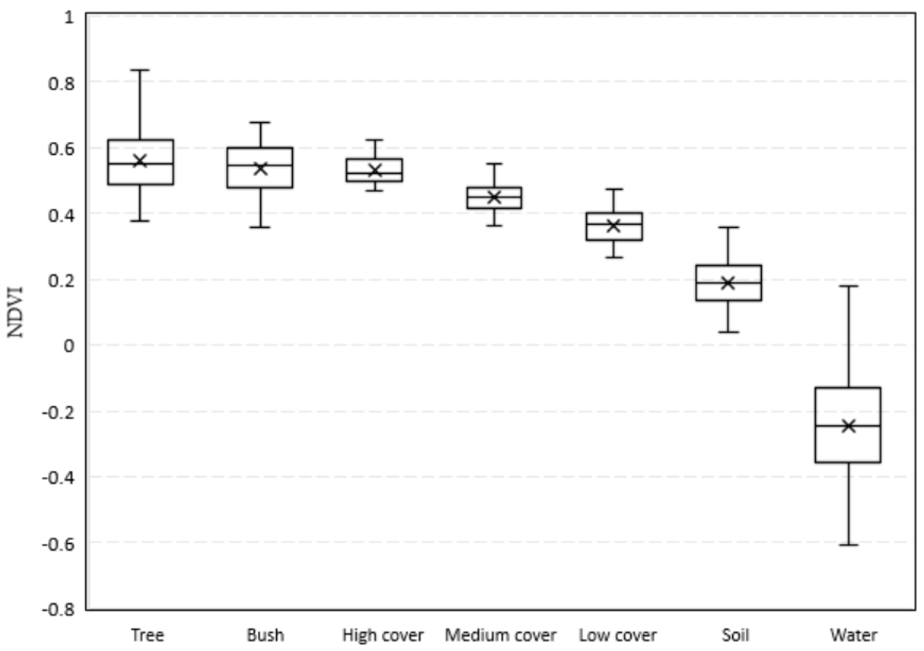
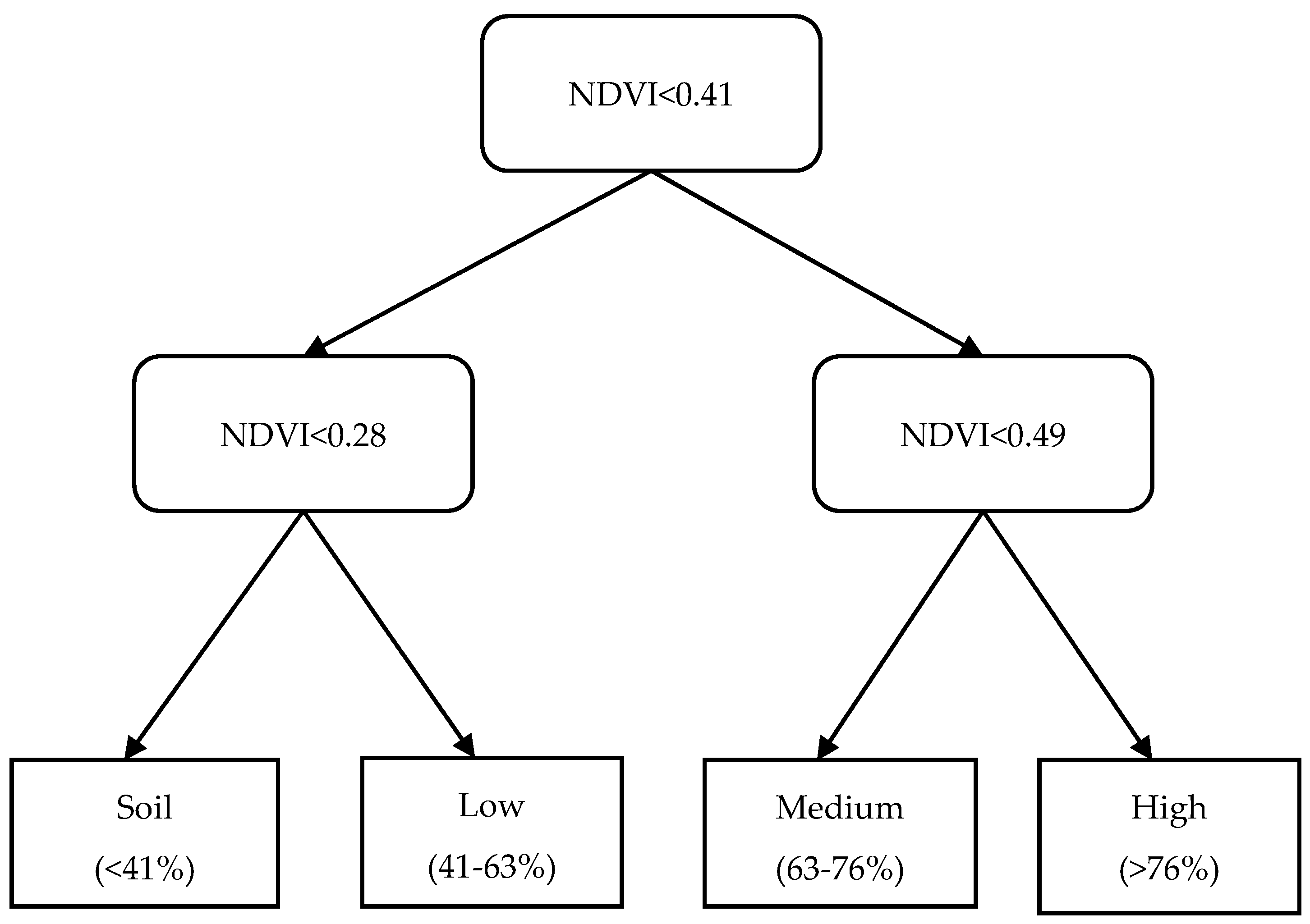
2.3.3. Decision Tree

It was noticed during the field survey that the grass coverage was not homogeneous. Thus, it is necessary to divide them into different categories to reflect the impacts of grazing management on grass coverage. The NDVI has been shown to have a good relationship with green vegetation coverage [40,41,42]. In order to distinguish different proportions of grass coverage, a decision tree based on the NDVI was used to categorize grass into high-, medium-, and low-cover, as well as bare soil. Using one of the most recognized algorithms [43], we have calculated the green vegetation fraction from the NDVI. The thresholds for low-, medium-, and high-coverage grass were 41%, 63%, and 76%, respectively.

To build the decision tree, about 6000 pixel samples of each class were selected in every pasture of different years via the region of interest (ROI) tool in ENVI. The samples were used to develop statistical relationships between the NDVI and different classes. Figure 3 shows that the potential of misclassifying the tree, shrub, and high-grass-cover categories due to overlap in the NDVI value range (Table S1); this demonstrates the necessity of classifying trees (through visual interpretation) and shrubs (through the SVM) separately before using the NDVI-based decision tree (Figure 2). From Figure 3, it is observed that the mean and range of the NDVI for the non-tree and non-shrub classes should be sufficient to distinguish high, medium, and low grass cover and soil with the NDVI-based decision tree. The average values of the NDVI increased from bare soil to high cover grass. NDVI cutoff values were the mean of the upper lower quartile of nearby two-class coverage. The decision tree used in this study is given in Figure 4.

2.4. Landscape Metrics and Statistical Analysis

Landscape metrics are a group of quantitative indices that can highly concentrate the information of landscape patterns and reflect the structural composition and spatial configuration of the landscape [44,45]. Landscape metrics can be used to show the status of classes in pastures, while interannual comparison of landscape metrics can show the changes caused by disturbances [46]. The land cover classification results were used to calculate the following landscape metrics for each year of NAIP data: class area (CA), number of patches (NP), class percentage of landscape area (PLAND), and fragmentation (FN) using the FRAGSTATS 4.2 [47]. The landscape metrics used in this study are shown in

Table 2. Landscape metrics used in this study. TA, CA, NP, PLAND, and FN represent total area, class area, number of patches, proportion of the landscape, and degree of fragmentation. The meaning of indices are as follows: i is class I, j is patch j in class I, m is the total class number, and n is the total patch number in class I.

Landscape index	Description	Formula
TA	Area of total landscape	$\mathit{T}\mathit{A}={\displaystyle \sum _{\mathit{i}=\mathbf{1}}^{\mathit{m}}}{\mathit{A}}_{\mathit{i}}$
CA	Area of class I	$\mathit{C}\mathit{A}={\mathit{A}}_{\mathit{i}}={\displaystyle \sum _{\mathit{i}=\mathbf{1}}^{\mathit{n}}}{\mathit{A}}_{\mathit{i}\mathit{j}}$
NP	Number of patches in class I	$\mathit{N}\mathit{P}={\mathit{N}}_{\mathit{i}}=\mathit{n}$
PLAND	Proportion of the landscape occupied by patch type (class) I	$\mathit{P}\mathit{L}\mathit{A}\mathit{N}\mathit{D}={\mathit{A}}_{\mathit{i}}/\mathit{A}$
FN	The degree of fragmentation of the class I	$\mathit{F}\mathit{N}={\mathit{N}}_{\mathit{i}}/{\mathit{A}}_{\mathit{i}}$

For the impacts of grazing treatments on grass, we focused on the grass coverage and NDVI value. Percentage of landscape (PLAND) for the four levels of grass cover (high cover, medium cover, low cover, and bare soil) and average NDVI of the grass category were compared between C and R in different years. For the impacts of grazing treatments on shrub distribution, we compared the shrub class metrics (area (CA), number of patches (NP), percentage of landscape (PLAND), and fragmentation (FN)) of the same pasture in different years. A paired-samples t-test was conducted to compare proportions of bare soil as well as low-, medium-, and high-coverage grass in continuous and rotational grazing treatments.

3. Results

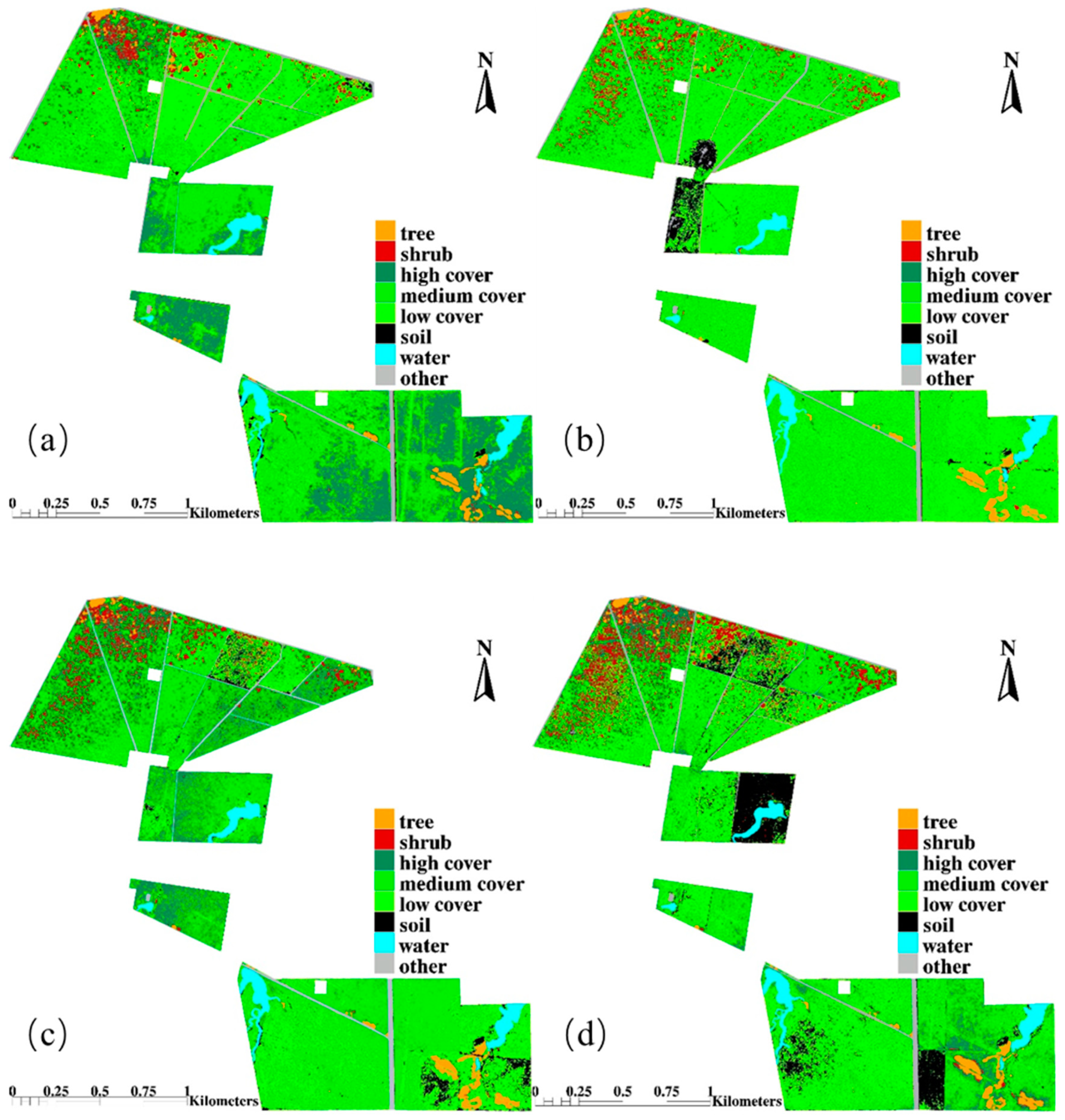
3.1. Land Cover Classification

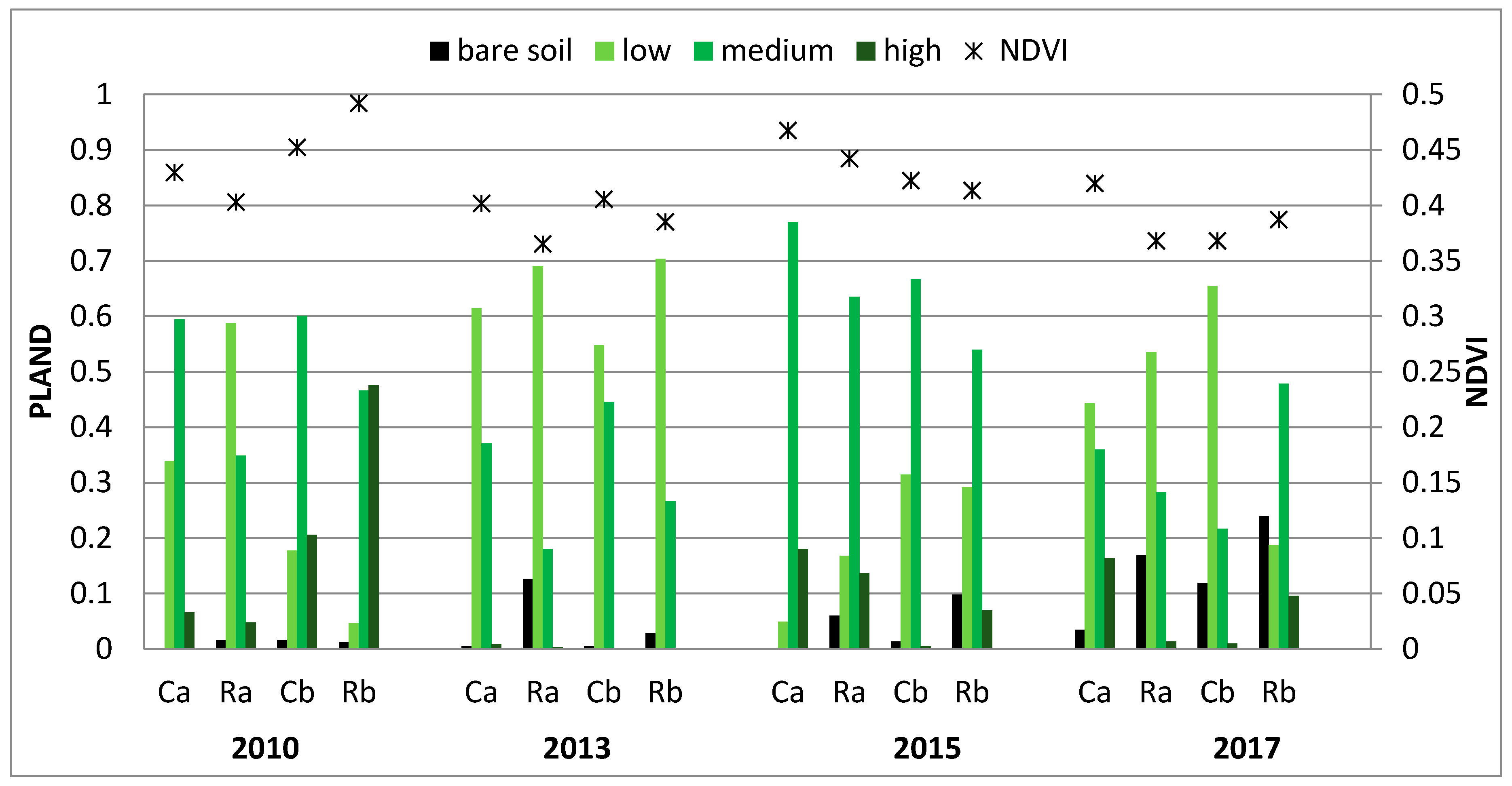
Land cover classification of the study area is shown in Figure 5. It is observed from Figure 5 that grass was clearly the dominant class in the landscape. Grass coverage of different pastures also largely differed within the same year, and grass coverage within pasture varied among years. Overall, grass in continuous pastures was more homogeneous (less mixture of different grass coverage classes) than rotational pastures, which had some bare soil in some of the paddocks (e.g., Figure 5b,d). The years 2010 and 2015 had better grass cover than other years, whereas grass coverage in 2013 was the poorest. Shrubs mainly occurred in Rep A, with scattered distribution, with a smaller number of shrubs in Rep B. Comparison of NAIP images from 2010 and 2017 indicate that shrubs increased in terms of number and area of patches in Ca and Ra while there were no visible changes in Cb and Rb. The dynamics of grass condition in different pastures is shown in Section 3.2, and shrub encroachment during these years is introduced in Section 3.3. Trees are generally concentrated along water bodies, with some scattered in the pastures and along old road beds. The proportion of trees showed little difference between years. The proportion of land area occupied by the water bodies varied slightly due to variation in rainfall.

3.2. Grass Dynamics

Fractional percent for four levels of grass coverage (high, medium, low, and bare soil) and the NDVI for both the continuous (C) and rotational (R) replicates (Rep A and Rep B) for 2010, 2013, 2015, and 2017 (Figure 6) were used to quantitatively investigate grass dynamics (refer to Tables S2–S5 for absolute values).

On a year-by-year basis, it is observed from Figure 6 that in 2010, Ca had more grassland that was classified as medium coverage (60%) compared to the low coverage (32%) or high coverage (5%) categories. In contrast to the Ca, the Ra replication had more area classified as low coverage (59%), which mainly occurred in sub-paddocks Ra1 to Ra4 (Figure 5a), and less in the medium coverage (35%) category. However, land area occupied by high grass cover was about the same as in Ca. The NDVI value was higher in Ca (0.43) than Ra (0.4). Cb had a lower NDVI value (0.45) than Rb (0.49). Cb exhibited less grass in the high category (20%) than Rb (48%), and more in the medium coverage category (60%) than in Rb (47%). Grass in Rep B was in better condition than in Rep A, shown by higher grass coverage and NDVI value in the former.

In 2013, the proportion of grass class classified as low grass coverage was highest in all four pastures among the four study years. The C pastures had higher percentages of grass classified as medium coverage (37–44%) than observed for the R pastures (18–26%). Little to no land area was classified as high coverage grass for any of the four pastures in this year. Comparatively, the R pastures had more land area classified as low coverage grass (~70%) than observed in the C pastures (55–63%). The C pastures showed a higher NDVI value (0.4) than the R pastures (0.36–0.37). It is also observed that for the R pastures during this year, more land was classified as bare soil than was observed in 2010. Pasture Ra exhibited much higher bare soil areas than Rb. Ra 10 and a small portion of Ra1, and Ra4 (Figure 5b) had large bare soil area.

In 2015, the C and R treatments all showed improved grass coverage over the prior years. The C pastures had larger percentages of grass classified as medium cover (66–78%) than observed in the R pastures (53–63%). Pastures Ca, Ra, and Rb had grass classified as high cover, but Cb had very little land area in this category. Cb and Rb had ~30% low cover grass, while Ca and Ra only had 5% and 16%, respectively. Bare soil was presented in both Ra (Ra3) and Rb (Rb2 and Rb3) (Figure 5c).

In 2017, the low-coverage grass category was highest in all replicates except Rb. Considering the medium- and high-coverage categories together, Ca had more area in these classes than Ra (51% versus 30%, respectively), while Cb had less area in these classes than Rb (20% versus 58%, respectively). The same trend was also found in the NDVI comparison between Ca and Ra (0.42 versus 0.37, respectively), and Cb and Rb (0.37 versus 0.39, respectively). Bare soil occurred in Ra2, Ra3, and Ra6. In the case of the Rb replicate, three sub-paddocks of Rb (Rb1, Rb7, and Rb8) contributed most to the total bare soil value (Figure 5d). A noticeable portion (12%) of pasture Cb was bare soil.

Table 3. Paired t-test results for four grass coverage categories in Rep A. The parameters t, df, and p represent t-statistic, degree of freedom, and the probability value for the t-statistic.

	t	df	p	Mean of the differences
Bare soil	−2.95	3	0.06	−0.08
Low grass cover	−3.38	3	0.04	−0.13
Medium grass cover	4.45	3	0.02	0.16
High grass cover	1.66	3	0.20	0.05

and

Table 4. Paired t-test results for four grass coverage categories in Rep B. Refer to Table 3. For the meaning of the parameters.

	t	df	p	Mean of the differences
Bare soil	−1.95	3	0.15	−0.06
Low grass cover	0.89	3	0.44	0.12
Medium grass cover	0.43	3	0.69	0.04
High grass cover	−1.83	3	0.17	−0.11

summarize the paired t-test results for four grass coverage categories in Reps A and B, respectively. There were significant differences (95% confidence interval) in the scores for Ca and Ra in low- and medium-grass-coverage categories (Table 3). However, there was no significant difference between Cb and Rb in any grass coverage category. These results suggest that the differences in grass coverage between rotational and continuous grazing were relatively small.

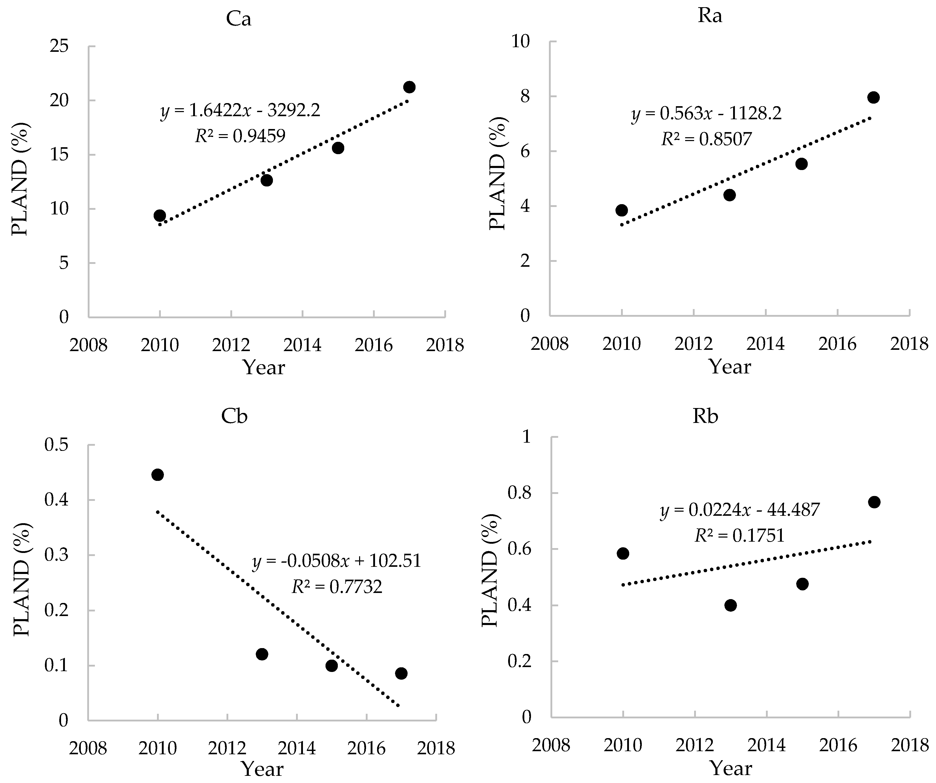
3.3. Shrub Encroachment

Table 5. Landscape metrics for shrub in the four pastures in the years 2010, 2013, 2015, and 2017.

ID	Year	TA (ha)	CA (ha)	PLAND (%)	NP	Patch Fragmentation
Ca	2010		5.49	9.37	1727	314.68
	2013	58.6	7.40	12.62	2054	277.69
	2015		9.15	15.61	2230	243.76
	2017		12.44	21.23	3034	243.87
Ra	2010		3.02	3.85	762	252.03
	2013	78.6	3.46	4.40	1266	365.79
	2015		4.35	5.54	1353	310.88
	2017		6.26	7.96	1438	229.88
Cb	2010		0.28	0.45	238	851.83
	2013	62.7	0.08	0.12	129	1710.88
	2015		0.06	0.10	93	1492.78
	2017		0.05	0.09	90	1679.10
Rb	2010		0.48	0.58	477	988.19
	2013	82.7	0.33	0.40	419	1268.54
	2015		0.39	0.47	331	842.88
	2017		0.63	0.77	346	545.40

includes landscape matrices for shrub in two treatments among the study years. Using the data presented in Table 5, the trend of shrub encroachment is analyzed with linear regressions between year and PLAND (Figure 7).

From Figure 7 it is readily observed that replicates Ca and Ra show increasing land area being encroached by shrubs, whereas the increase in shrub area is minimal in Rb and slightly decreased in Cb. The shrub encroachment was consistent among years in Ca, while there was a turning point at year 2013 in Ra, which indicates that shrub area was increasing slowly before 2013 and had a larger increasing rate after that. In 2010, the shrub area was 9% of the land area in Ca and 4% in Ra. By 2017, the shrub area had increased 12% in Ca and 4% in Ra. From 2010 to 2017, the number of patches and the area occupied by shrub (NP and CA in Table 2) increased in both Ca and Ra. However, patch fragmentation decreased, indicating that the patches were growing in size and beginning to cluster together. The linear regressions (r² = 0.94 and 0.85 for Ca and Ra, respectively) reveal that by the year 2030, if shrub encroachment is not addressed, potentially 24 ha (41%) of Ca may be occupied by shrubs, and that shrubs may account for 11.8 ha (15%) of the land area of Ra.

As mentioned earlier, both the initial proportion (less than 1%) and dynamics of shrubs were small in Cb and Rb. Shrubs only occupied a minimal portion of Cb, and can almost be ignored after 2015. A turning point appeared in 2013, which means the shrub area changing rate decreased after 2013. In 2010, shrub PLAND was only ~0.5%, and this value was less than 0.1% by 2017. Patch fragmentation increased during 2010 to 2017. The linear regressions (r² = 0.77) implies that shrub will disappear in Cb after 2018. In pasture Rb, the shrub area decreased from 2010 to 2013, then increased after 2013. On the contrary, patch fragmentation increased first, then decreased after 2013. The increasing shrub was mainly contributed by newly growing small woody trees distributed around existing trees (Figure 5).

4. Discussion

Grass interannual dynamics were jointly controlled by climate conditions and grazing management. In 2013, worse grass conditions were caused by severe drought in 2011 and 2012, although the region had good temperature (T) and precipitation (P) (Figure S2). However, Zhou et al. [48] indicate that grass productivity in 2013 was high, which means grass grew well after the imaging date. With good T and P in May and June 2015, grass coverage and NDVI of all pastures improved over 2013, and Rep A had the best grass condition during the study period. However, grass condition of Rb in 2015 was not better than in 2010, with less high-coverage area and a lower NDVI; this is probably because Rep B was not grazed in 2010. The climate was similar in years 2017 and 2015, but the imaging date was a half-month earlier in 2017. Thus, there was higher percentage of low-coverage grass in 2017 than in 2015, due to a shorter growing period until image acquisition date in the former. Rb had highest medium coverage area, because of most sub-paddocks were rested.

Shrub encroachment rates between years indicated that climate was a key factor controlling shrub encroachment. In harsh climate conditions, shrub might die. Because of previous consecutive drought in 2011 and 2012, the shrub encroachment rate in Rep A was the slowest from 2010 to 2013; meanwhile, shrub area decreased in Rep B. After that, the climate conditions were less harsh, and the shrub encroachment was faster in Rep A. The shrub distribution in Rb also increased after 2013. In contrast, the shrub area continued to decrease in Cb at a much lower rate, probably because the area was too small and isolated distribution made it easy to be destroyed by cattle. Initial shrub area and distribution in pastures was another key factor in determining shrub encroachment. Rep A had large shrub encroachment, with a high proportion of shrub area and small patch fragmentation at the beginning of the experiment. Rep B, which had a small number of shrub area and high patch fragmentation at the beginning of the experiment, showed little change in shrub distribution.

Our results showed that grazing management affected grass coverage and is not a significant factor in controlling shrub encroachment. However, since NAIP images were snapshots in the early growing season, they cannot represent the grass condition for the whole grazing season. Thus, it is hard to evaluate how the grazing management affected grass production between years, because of low temporal resolution of NAIP images. The high stocking intensity created bare soil in some of paddocks in R pastures, which indicates that high grazing intensity in rotational grazing can cause the late growth of grasses. However, vegetation growth might be better later in the year and compensate for the damage caused by intensive grazing when grazing pressure is removed. As we found, Ca had better grass condition than Ra. Zhou et al. [48] studied grass productivity and did not show an advantage in Ca. More frequent observation is needed to better evaluate grazing management at annual scale. Soil type is also an important factor in affecting grass condition. Before grazing started, Rb had better grass condition than Cb. However, Cb had better grass condition than Rb in 2013 and 2015 after grazing, but also had the grass condition among pastures in 2017. Grass condition getting worse in Cb might be because of poor soil fertility, which cannot support recovery from grazing.

5. Conclusions

The comparison between paddocks in the same year showed that high grazing intensity in rotational grazing can cause the late growth of grasses. Ca always had better overall vegetation growth than Ra. Cb had a better vegetation growth than Rb at the beginning of the experiment (2013). However, their respective growth was similar in 2015, and Rb outperformed Cb in 2017, which indicates that soil fertility in Cb might not have been enough to support the grass recovery at current grazing pressure. The grass condition had large variation and no trend within study years. In the years with good T and P, grass recovered faster. To sum up, grass coverage was jointly affected by grazing management (stocking intensity) and climate.

Climate and initial status of shrub distribution (total area, percentage of landscape, fragmentation) instead of grazing management were the controlling factors of shrub encroachment. Higher initial proportion and better climate facilitated shrub encroachment. Shrub encroachment at a rapid speed in pasture Ca may cover 40% of the land area in 2030, and 15% of the land area in Ra. Scattered distribution of low-percentage shrub might even get suppressed. It is hard to conclude how grazing management affects shrub encroachment. Both high spatial and temporal resolution images are required to better monitor the tallgrass prairie landscapes.

References

1. Samson, F.B.; Knopf, F.L.; Ostlie, W.R. Great Plains ecosystems: past, present, and future. Wildl. Soc. 2004, 32, 6–15. [Google Scholar] [CrossRef] [Green Version]
2. Cunfer, G. On the Great Plains: Agriculture and Environment; Texas A&M University Press: College Station, TX, USA, 2005. [Google Scholar]
3. Fuhlendorf, S.D.; Engle, D.M. Restoring Heterogeneity on Rangelands: Ecosystem Management Based on Evolutionary Grazing Patterns: We propose a paradigm that enhances heterogeneity instead of homogeneity to promote biological diversity and wildlife habitat on rangelands grazed by livestock. BioScience 2001, 51, 625–632. [Google Scholar]
4. Westoby, M.; Walker, B.; Noy-Meir, I. Opportunistic Management for Rangelands Not at Equilibrium. J. Range Manag. 1989, 42, 266. [Google Scholar] [CrossRef]
5. Bidwell, T.; Elmore, D.; Hickman, K. Stocking Rate Determination on Native Rangeland. Available online: https://www.cattlemen.bc.ca/docs/factsheet_stocking_rate_determination.pdf (accessed on 25 March 2019).
6. Hubbard, W.A. Rotational Grazing Studies in Western Canada. J. Range Manag. 1951, 4, 25. [Google Scholar] [CrossRef]
7. Hyder, D.N.; Sawyer, W.A. Rotation-Deferred Grazing as Compared to Season-Long Grazing on Sagebrush-Bunchgrass Ranges in Oregon. J. Range Manag. 1951, 4, 30. [Google Scholar] [CrossRef]
8. McIlvain, E.H.; Savage, D.A. Eight-Year Comparisons of Continuous and Rotational Grazing on the Southern Plains Experimental Range. J. Range Manag. 1951, 4, 42. [Google Scholar] [CrossRef]
9. Rogler, G.A. A Twenty-Five Year Comparison of Continuous and Rotation Grazing in the Northern Plains. J. Range Manag. 1951, 4, 35. [Google Scholar] [CrossRef]
10. Sampson, A.W. A Symposium on Rotation Grazing in North America. J. Range Manag. 1951, 4, 19. [Google Scholar] [CrossRef]
11. Norton, B.E.; Barnes, M.; Teague, R. Grazing Management Can Improve Livestock Distribution. Rangelands 2013, 35, 45–51. [Google Scholar] [CrossRef]
12. Eldridge, D.J.; Soliveres, S.; Bowker, M.A.; Val, J. Grazing dampens the positive effects of shrub encroachment on ecosystem functions in a semi-arid woodland. J. Appl. Ecol. 2013, 50, 1028–1038. [Google Scholar] [CrossRef] [Green Version]
13. Heady, H.F. Continuous vs. Specialized Grazing Systems: A Review and Application to the California Annual Type. J. Range Manag. 1961, 14, 182. [Google Scholar] [CrossRef]
14. Teague, W.; Dowhower, S.; Baker, S.; Haile, N.; Delaune, P.; Conover, D. Grazing management impacts on vegetation, soil biota and soil chemical, physical and hydrological properties in tall grass prairie. Agric. Ecosyst. 2011, 141, 310–322. [Google Scholar] [CrossRef]
15. Teague, R.; Provenza, F.; Kreuter, U.; Steffens, T.; Barnes, M. Multi-paddock grazing on rangelands: Why the perceptual dichotomy between research results and rancher experience? J. Environ. Manag. 2013, 128, 699–717. [Google Scholar] [CrossRef] [PubMed]
16. Bryant, F.C.; Dahl, B.E.; Pettit, R.D.; Britton, C.M. Does short-duration grazing work in arid and semiarid regions? J. Soil Water Conserv. 1989, 44, 290–296. [Google Scholar]
17. Gillen, R.L.; Mccollum, F.T.; Tate, K.W.; Hodges, M.E. Tallgrass Prairie Response to Grazing System and Stocking Rate. J. Range Manag. 1998, 51, 139. [Google Scholar] [CrossRef]
18. Briske, D.D.; Derner, J.D.; Brown, J.R.; Fuhlendorf, S.D.; Teague, W.R.; Havstad, K.M.; Gillen, R.L.; Ash, A.J.; Willms, W.D. Rotational Grazing on Rangelands: Reconciliation of Perception and Experimental Evidence. Rangel. Ecol. Manag. 2008, 61, 3–17. [Google Scholar] [CrossRef]
19. Budd, B.; Thorpe, J. Benefits of Managed Grazing: A Manager’s Perspective. Rangelands 2009, 31, 11–14. [Google Scholar] [CrossRef]
20. Briske, D.D.; Sayre, N.F.; Huntsinger, L.; Fernandez-Gimenez, M.; Budd, B.; Derner, J.D. Origin, Persistence, and Resolution of the Rotational Grazing Debate: Integrating Human Dimensions Into Rangeland Research. Rangel. Ecol. Manag. 2011, 64, 325–334. [Google Scholar] [CrossRef]
21. Becker, W.; Kreuter, U.; Atkinson, S.; Teague, R. Whole-Ranch Unit Analysis of Multipaddock Grazing on Rangeland Sustainability in North Central Texas. Rangel. Ecol. Manag. 2017, 70, 448–455. [Google Scholar] [CrossRef]
22. Danvir, R.; Simonds, G.; Sant, E.; Thacker, E.; Larsen, R.; Svejcar, T.; Ramsey, D.; Provenza, F.; Boyd, C. Upland Bare Ground and Riparian Vegetative Cover Under Strategic Grazing Management, Continuous Stocking, and Multiyear Rest in New Mexico Mid-grass Prairie. Rangelands 2018, 40, 1–8. [Google Scholar] [CrossRef]
23. Sampson, A.W. Range Improvement by Deferred and Rotation Grazing; Bulletin of the U.S. Department of Agriculture No. 34: Washington, DC, USA, 1913. [Google Scholar]
24. Leo, B.M. A Variation of Deferred Rotation Grazing for Use under Southwest Range Conditions. J. Range Manag. 1954, 7, 152–154. [Google Scholar]
25. White, M.R.; Pieper, R.D.; Donart, G.B.; Trifaro, L.W. Vegetational Response to Short-Duration and Continuous Grazing in Southcentral New Mexico. J. Range Manag. 1991, 44, 399. [Google Scholar] [CrossRef]
26. Jacobo, E.J.; Rodriguez, A.M.; Bartoloni, N.; Deregibus, V.A. Rotational Grazing Effects on Rangeland Vegetation at a Farm Scale. Rangelands 2006, 59, 249–257. [Google Scholar] [CrossRef]
27. Wang, T.; Teague, W.R.; Park, S.C. Evaluation of Continuous and Multipaddock Grazing on Vegetation and Livestock Performance—a Modeling Approach. Rangel. Ecol. Manag. 2016, 69, 457–464. [Google Scholar] [CrossRef]
28. Van Auken, O.W. SHRUB INVASIONS OF NORTH AMERICAN SEMIARID GRASSLANDS. Annu. Ecol. Syst. 2000, 31, 197–215. [Google Scholar] [CrossRef]
29. Knapp, A.K.; Briggs, J.M.; Collins, S.L.; Archer, S.R.; Ewers, B.E.; Peters, D.P.; Young, D.R.; Shaver, G.R.; Pendall, E.; Cleary, M.B.; et al. Shrub encroachment in North American grasslands: shifts in growth form dominance rapidly alters control of ecosystem carbon inputs. Chang. Boil. 2008, 14, 615–623. [Google Scholar] [CrossRef]
30. Angell, D.L.; McClaran, M.P. Long-term influences of livestock management and a non-native grass on grass dynamics in the Desert Grassland. J. Environ. 2001, 49, 507–520. [Google Scholar] [CrossRef]
31. Batáry, P.; Orci, K.M.; Báldi, A.; Kleijn, D.; Kisbenedek, T.; Erdős, S. Effects of local and landscape scale and cattle grazing intensity on Orthoptera assemblages of the Hungarian Great Plain. Basic Appl. Ecol. 2007, 8, 280–290. [Google Scholar] [CrossRef]
32. Schönbach, P.; Wan, H.; Gierus, M.; Bai, Y.F.; Müller, K.; Lin, L.J.; Susenbeth, A.; Taube, F. Grassland responses to grazing: Effects of grazing intensity and management system in an Inner Mongolian steppe ecosystem. Plant Soil 2011, 340, 103–115. [Google Scholar] [CrossRef]
33. Baldi, A.; Batary, P.; Kleijn, D. Effects of grazing and biogeographic regions on grassland biodiversity in Hungary—Analysing assemblages of 1200 species. Agric. Ecosyst. 2013, 166, 28–34. [Google Scholar] [CrossRef]
34. NAIP Imagery. Available online: https://www.fsa.usda.gov/programs-and-services/aerial-photography/imagery-programs/naip-imagery (accessed on 20 March 2018).
35. U.S. Department of Agriculture, Natural Resources Conservation Service. National soil survey handbook, title 430-VI. Available online: http://www.nrcs.usda.gov/wps/portal/nrcs/detail/soils/ref/?cid=nrcs142p2_054242 (accessed on 20 March 2019).
36. Steiner, J.L.S.; Neel, P.J.; Northup, B.K.; Gowda, P.H.; Brown, M.A.; Coleman, S. Managing, Tallgrass Prairies for Productivity and Ecological Function: A Long Term Grazing Experiment in the Southern Great Plains, USA. Agronomy 2019. In press. [Google Scholar]
37. Tucker, C.J. Red and photographic infrared linear combinations for monitoring vegetation. Remote. Sens. Environ. 1979, 8, 127–150. [Google Scholar] [CrossRef] [Green Version]
38. Cortes, C.; Vapnik, V. Support-vector networks. Mach. Learn. 1995, 20, 273–297. [Google Scholar] [CrossRef] [Green Version]
39. Pal, M.; Mather, P.M. Support vector machines for classification in remote sensing. Int. J. Sens. 2005, 26, 1007–1011. [Google Scholar] [CrossRef]
40. DeFries, R.S.; Townshend, J.R.G. NDVI-derived land cover classifications at a global scale. Int. J. Sens. 1994, 15, 3567–3586. [Google Scholar] [CrossRef]
41. Carlson, T.N.; Ripley, D.A. On the relation between NDVI, fractional vegetation cover, and leaf area index. Remote. Sens. Environ. 1997, 62, 241–252. [Google Scholar] [CrossRef]
42. Geerken, R.; Zaitchik, B.; Evans, J.P. Classifying rangeland vegetation type and coverage from NDVI time series using Fourier Filtered Cycle Similarity. Int. J. Sens. 2005, 26, 5535–5554. [Google Scholar] [CrossRef] [Green Version]
43. Gutman, G.; Ignatov, A. The derivation of the green vegetation fraction from NOAA/AVHRR data for use in numerical weather prediction models. Int. J. Sens. 1998, 19, 1533–1543. [Google Scholar] [CrossRef]
44. Wagner, H.H.; Fortin, M.-J. Spatial Analysis of Landscapes: Concepts and Statistics. Ecology 2005, 86, 1975–1987. [Google Scholar] [CrossRef]
45. McGarigal, K. Landscape Pattern Metrics. Available online: https://www.umass.edu/landeco/pubs/mcgarigal.2002.pdf (accessed on 12 October 2018).
46. Fichera, C.R. Land Cover classification and change-detection analysis using multi-temporal remote sensed imagery and landscape metrics. Eur. J. Sens. 2012, 45, 1–18. [Google Scholar] [CrossRef] [Green Version]
47. McGarigal, K.; Marks, B.J. Fragstats: Spatial Pattern Analysis Program for Quantifying Landscape Structure; U.S. Department of Agriculture, Forest Service, Pacific Northwest Research Station: Corvallis, OR, USA, 1995; Volume 351, p. 122.
48. Zhou, Y.; Gowda, P.H.; Wagle, P.; Ma, S.; Neel, J.P.S.; Kakani, V.G.; Steiner, J.L. Climate Effects on Tallgrass Prairie Responses to Continuous and Rotational Grazing. Agronomy 2019, 9, 219. [Google Scholar] [CrossRef]
Figure 1. The study area with the National Agriculture Imagery Program (NAIP) mosaic true color image as background. The location of the study site within the state of Oklahoma is shown in the inset.
Agronomy 09 00238 g001
Figure 2. Flow of the land cover classification.
Agronomy 09 00238 g002
Figure 3. Normalized Difference Vegetation Index (NDVI) box-plot diagram for each category.
Agronomy 09 00238 g003
Figure 4. NDVI-based decision tree. The percentage in the lower box represents the green vegetation fraction for corresponding grass class.
Agronomy 09 00238 g004
Figure 5. Land classification results in 2010 (a), 2013 (b), 2015 (c), and 2017 (d).
Agronomy 09 00238 g005
Figure 6. NDVI and fractional percent of grass coverage (bare soil, low coverage, medium coverage, and high coverage) for 2010, 2013, 2015, and 2017.
Agronomy 09 00238 g006
Figure 7. Shrub PLAND by year for each replicate (Ca, Ra, Cb and Rb).
Agronomy 09 00238 g007