Article

Modeling Carbon and Water Fluxes of Managed Grasslands: Comparing Flux Variability and Net Carbon Budgets between Grazed and Mowed Systems

1
INRA, Versailles-Grignon, UMR ECOSYS, Bâtiment EGER, 78850 Thiverval-Grignon, France
2
Rothamsted Research, Department of Plant Sciences, West Common, Harpenden, Herts AL5 2JQ, UK
3
INRA UMR 1069 SAS, 65 rue de Saint-Brieuc, 35042 Rennes, France
4
INRA, VetAgro Sup, UMR 874 Ecosystème Prairial, 63100 Clermont Ferrand, France
5
Manaaki Whenua—Landcare Research, Private Bag 11052, Palmerston North 4442, New Zealand
6
INRA, Centre de recherche Nouvelle-Aquitaine-Poitiers, URP3F, 86600 Lusignan, France
*
Author to whom correspondence should be addressed.
Agronomy 2019, 9(4), 183; https://doi.org/10.3390/agronomy9040183
Submission received: 2 March 2019 / Revised: 2 April 2019 / Accepted: 7 April 2019 / Published: 10 April 2019
(This article belongs to the Special Issue Grassland Management for Sustainable Agroecosystems)

Abstract

:
The CenW ecosystem model simulates carbon, water, and nitrogen cycles following ecophysiological processes and management practices on a daily basis. We tested and evaluated the model using five years eddy covariance measurements from two adjacent but differently managed grasslands in France. The data were used to independently parameterize CenW for the two grassland sites. Very good agreements, i.e., high model efficiencies and correlations, between observed and modeled fluxes were achieved. We showed that the CenW model captured day-to-day, seasonal, and interannual variability observed in measured CO2 and water fluxes. We also showed that following typical management practices (i.e., mowing and grazing), carbon gain was severely curtailed through a sharp and severe reduction in photosynthesizing biomass. We also identified large model/data discrepancies for carbon fluxes during grazing events caused by the noncapture by the eddy covariance system of large respiratory losses of C from dairy cows when they were present in the paddocks. The missing component of grazing animal respiration in the net carbon budget of the grazed grassland can be quantitatively important and can turn sites from being C sinks to being neutral or C sources. It means that extra care is needed in the processing of eddy covariance data from grazed pastures to correctly calculate their annual CO2 balances and carbon budgets.

1. Introduction

Managed grasslands and rangelands represent ~70% of global agricultural area [1], which is 25% of the Earth’s ice-free land surface [2]. The soils of these agroecosystems contain ~20% of the world’s soil organic carbon (SOC) stocks, which implies that they play a significant role in the global carbon and water cycles [3,4,5,6,7]. In Europe, grasslands cover 22% of the land area [8], where management practices and climate strongly influence their C sequestration rates. Average annual estimates of carbon balances of temperate grasslands for EU countries ranged from being a C source of 45 kg C ha−1 year−1 to a C sink of 400 kg C ha−1 year−1 [9]. Hence, these managed agroecosystems may contribute to the mitigation of climate change [7,10,11,12]. However, these ecosystems are particularly complex and difficult to investigate because of the wide range of management and environmental conditions that they are exposed to, leading to a large variability in their CO2 source/sink capacity [5,13,14,15,16,17].
Most of the vegetation growing on pastoral lands is used to either feed animals directly (grazing), or it is harvested and used to feed animals at other times or locations (mowing). Grasslands managed through mowing are fundamentally different to grassland managed through grazing with respect to their above ground biomass removal patterns, export and cycling of carbon, and applications of fertilizer, as more nitrogen is returned to the field during grazing through animals excreta compared to mowing where almost everything is exported from the system [15,18]. In addition, there is large uncertainties about the effects of mowing and grazing on different ecological processes related to their C cycle [16,19,20].
The frequency and intensity of foliage removal and its fate (grazed on site or mowed and exported) have effects on the carbon budgets but also on the nutrient cycling and development of the grassland [7,21,22]. Grazing intensity showed to have significant effect on the soil carbon sequestration potential of grassland ecosystems. Positive C sequestration was reported for light-to-moderate grazing intensities [11,23], while overgrazing or trampling were found to have a negative effect on SOC stocks [24]. Although less studied than grazing systems [25], mowing is usually related to important losses of soil organic carbon unless manure is returned to the paddock because of the export of biomass from the grassland that reduces the amount of C inputs to the agroecosystem [26]. However, previous studies found that soil carbon stocks of mowed grassland could also increase depending on the cutting/harvesting intensity [8,18].
Direct and accurate measurements of small changes in soil organic carbon stocks over short time periods in response to different management practices are difficult to achieve because of the large spatial variability of SOC and of the large C content of the soil relative to the rate of change [27,28,29]. Despite the uncertainties associated with flux measurements, eddy covariance (EC) is a powerful tool for measuring ecosystem/atmosphere carbon fluxes [8,30,31,32]. With EC, it is possible to detect changes in net ecosystem exchange (NEE) of carbon at a half-hourly time resolution, which enables estimates to be made of whether land management practices result in systems being net sinks or sources of CO2 [12,26]. NEE is the balance of gross primary production (GPP) and ecosystem respiration (ER) and it represents the net exchange of CO2 between the atmosphere and terrestrial ecosystems. For managed ecosystems, the carbon balance has to comprise NEE and C losses (harvested biomass, enteric fermentation, export of animal products, and organic and inorganic C losses through leaching and erosion) as well as nonphotosynthetic carbon gains (organic fertilization), resulting in the net biome productivity (NBP = NEE + carbon export − carbon import (positive value indicates that the ecosystem is a carbon source). NEE is a key variable to determine the carbon balance of an ecosystem and therefore, understanding it responses to environmental change, management, and site characteristics is essential [33,34,35]. Over seasonal and interannual time scales, NEE in managed grasslands can vary with the frequency, timing and duration of management practices. Mowing and grazing removes photosynthesizing biomass and can thereby temporarily but substantially reduce GPP [18,36,37].
To develop a better understanding of ecosystem processes, or predict the response of ecosystem to climate change and management practices, various process-based (mechanistic) vegetation models have been developed [38,39,40]. They vary in complexity and can operate at different temporal and spatial scales. They are being used widely to simulate ecosystem carbon and nitrogen dynamics. The reliability of these models highly depend on the quantity and quality of the data used for their calibration [41,42,43]. Model parameters calibration aims to constrain the uncertainty in model parameter space and optimize the model output of ecosystem–atmosphere CO2 exchange [44]. Measured CO2 fluxes were used to constrain model simulation through parameter calibration. Once parameterized, these models allow to simulate separately the constituents of NEE (soil, microbial, plant, and animal respiration and gross primary production) that cannot be measured directly by EC, or to interpolate and extrapolate CO2 fluxes in time and space. However, insufficient knowledge about underlying processes (e.g., all the processes leading to observed carbon and water fluxes and flows that exists in the real world but are not or are only poorly understood and modeled) as well as parameters and initial conditions uncertainties can lead to bias and uncertainty in model simulations [45]. Also, because interannual responses are usually less well captured by models than daily and seasonal dynamics [46,47,48], the availability and quality of long-term datasets are crucial to improve model performances [49]. Process-based simulation models are therefore required to gain insight of processes and interactions between managed grasslands C dynamics, climate change, and management practices, in combination with experimental observations, especially for long-term analyses [50,51].
CenW (carbon, energy, nutrients, and water) is a process-based model, running at a daily time step. It was originally developed to simulate the carbon balance of forests over time [52,53,54]. The soil organic matter module of the model was derived from the CENTURY model [55], which was originally developed for grasslands (more details are given in Section 2.2). Recently, CenW was successfully parameterized and used to simulate carbon and water fluxes of an intensively grazed dairy pasture in New Zealand [56], and to test effects of different climate and management practices on soil carbon stocks and milk production [57].
In this study, we used the CenW model to simulate the seasonal and interannual variability of carbon dioxide and water fluxes of two differently managed grassland fields located in France. The two selected paddocks are part of the Agroecosystem Biogeochemical Cycles and Biodiversity (ACBB) long-term national research infrastructure. They are located only 200 meters apart and are equipped with eddy covariance (EC) flux towers. These sites were either regularly mowed or grazed, and they received different fertilizer doses applied following different application patterns. Within the framework of this study, we focused on the differences between carbon and water fluxes between grasslands under mowing and grazing managements. Flux data from the paired paddocks were used to parameterize and validate the CenW model.
The specific objectives of the present study were to
  • test the ability of the CenW model to simulate water and CO2 flux dynamics of two temperate grassland ecosystems under mowing and grazing management, respectively;
  • evaluate the model’s ability to capture the seasonal and interannual dynamics of CO2 and water fluxes in response to climate variability (five years) in interaction with two contrasting management practices (mowing and grazing); and
  • determine the effects of mowing and grazing on eddy covariance fluxes and on the CO2 budget of managed grasslands.

2. Materials and Methods

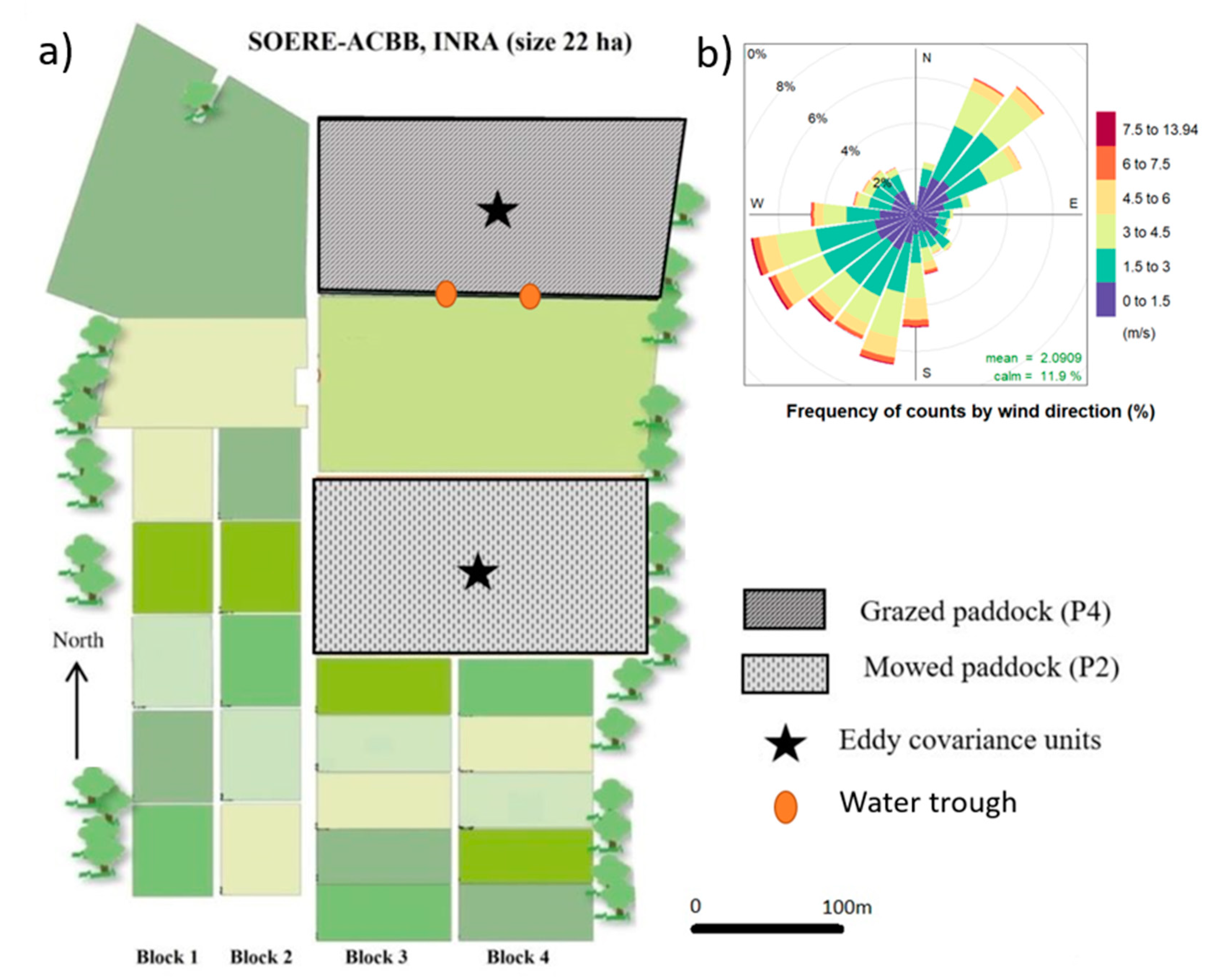
2.1. Experimental Details

The experimental site is located at the Lusignan INRA (National Institute for Agricultural Research) experimental farm, France (46°25′12.91″ N; 0°07′29.35″ E), which covers ~22 ha (Figure 1). INRA and CNRS (National Centre for Scientific Research) jointly designed the long-term observational study to gain a better understanding of the environmental impacts resulting from different grassland management practices and grassland/cropping rotations. The study site was established on temporary grasslands that were sown in spring 2005 (March–April). Before 2005, part of the observational site was grassland, and the other part was alternated between grass and crop rotations for 17 years. The total surface area of the experimental site was ploughed to establish a base line for the system before sowing grass in 2005. The upper soil horizons are characterized by a loamy texture, classified as Cambisol, whereas lower soil horizons have a clayey texture rich in kaolinite and iron oxides, classified as a Paleo-Ferralsol [58,59]. The sown grasslands consisted of a mix of three grass species (Lolium perenne, Festuca arundinacea, and Dactylis glomerata L.). For the original experiment, the 22 ha of the study area were divided into four blocks of five 0.4 ha plots and four larger plots of 3 ha to test seven different treatments (shown in different colors in Figure 1) [60]. The treatments relevant for the present work are two of the 3 ha plots with pasture being either mowed or grazed. The towers footprints are crucial in experimental set up of eddy covariance and a detailed footprint study was performed [26]. The wind rose, which is identical for the two paddocks, is reported in Figure 1. Footprint analysis indicated that ~70% of the median percentage of the footprint was in the field, which is a similar fraction than that found in other similar studies [26].
For the present study, two temporary sown grasslands paddocks, each of a size of ~3 ha and of rectangular shape, were equipped with two eddy covariance measurement systems and a meteorological station (Figure 1). One of the paddocks was regularly mowed (P2), with harvested hay exported off-site to feed animals during periods of insufficient vegetation growth (mainly drought periods and during winter). Dairy cows regularly grazed the other paddock (P4), with all animal excreta directly returned to the paddock, except for the fraction that was deposited off site during milking and during the daily transit times from the milking shed to the field. Both paddocks received regular applications of nitrogen fertilizer, with higher rates applied to the mowed than the grazed paddock (Appendix A).
For the two contrasting grassland systems studied here, the dates of mowing and grazing, the length of each grazing event, the animal stocking densities, and timing and amounts of N fertilizer applications varied in the different years. Details are given in Appendix A. Over the 5-year study period (2006–2010) the mowed paddock received 1290 kg N ha−1 split into 17 fertilizer applications and was mowed 17 times with 3 cuts per year, except for the wetter than normal summer half-year 2007 (5 cuts). Over the same period, the grazed paddock received 590 kg N ha−1 (not including N returned in dung and urine during grazing) over 14 applications and was grazed 37 times with grazing events spread, on average, over 5 consecutive days.

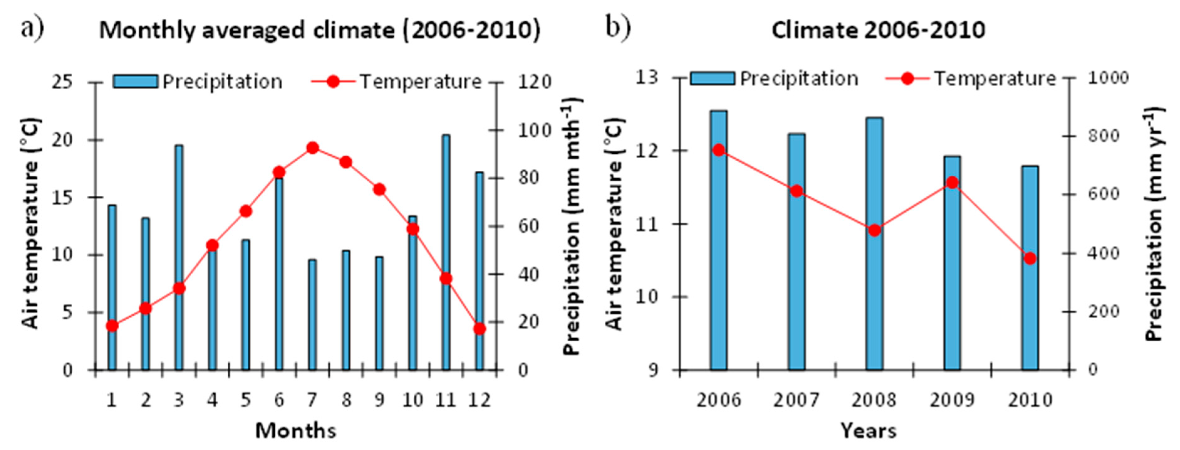
2.1.1. Meteorological Conditions at the Study Site

Meteorological conditions for the two paddocks were acquired from a weather station coupled to a data logger (CR-10X, Campbell Scientific Inc., Logan, UT) placed 1.9 meters aboveground on the mown paddock [17,26,61]. Briefly, the weather station provided 30 min averaged values of precipitation (SBS500, Campbell Scientific Inc., Logan, UT), air temperature and relative humidity (HMP 45 AC, Vaisala), radiation components (CNR1, Kipp & Zonen), and wind speed (A100L2, Vector Instruments) and direction (W200P, Vector Instruments). Volumetric soil water content data were collected by time domain reflectometry (TDR) probes at 10, 20, 30, 60, 80, and 100 cm depths (CS616, Campbell Scientific Inc., Logan, UT), and soil temperatures were measured at 5, 10, 20, 30, 60, 80, and 100 cm down the soil profile (PT100, Mesurex), but only for the mowed paddock. Soil heat flux was measured at 5-cm-depth (HFP01, Hukseflux), and data were corrected for changes in heat storage in the soil layer above the flux plate [62]. Over the study period (2006–2010), average air temperature and average annual precipitation were 11.2 °C and 774 mm yr−1, respectively. Half-hourly meteorological data, i.e., air temperature, global radiation, humidity, and precipitation, were summed/averaged to daily values to be used as driving variables for the CenW model runs of both paddocks.
The predominant wind direction was from the southwest and a secondary peak from the northeast (Figure 1b).
Throughout the five years of the study, daily maximum air temperature exceeded 25 °C for 10.5% of the time, with a maximum of 35.5 °C. Daily minimum air temperature was negative for 13.3% of the time, with a lowest value of −11.0 °C (data not shown). Summer months (June–September) were hot and dry with average monthly air temperature ranging between 15.6 and 19.4 °C and precipitations between 48 and 71 mm mth−1 (Figure 2a). The wettest and coldest month are November (98 mm mth−1) and December (3.6 °C), respectively (Figure 2a). Among the five years of the study, 2006 was the warmest (11.9 °C) and wettest (888 mm yr−1), while 2010 was the coldest (10.5 °C) and driest (697 mm yr−1) year.

2.1.2. Eddy Covariance (EC) Measurements and Processing

We used paired eddy covariance systems for the 2006–2010 period because it provided EC data measurements for both mowed (P2) and grazed (P4) paddocks. The two EC systems recorded raw data at 20 Hz, and EddyPro® software (LI-COR Inc.) was used for postprocessing and the calculation at 30-minute intervals for fluxes of CO2, momentum, and sensible and latent heat. Each EC unit included a fast response sonic anemometer (Solent R3-50; Gill Instrument, Lymington, UK) and an open-path CO2-H2O infrared gas analyzer (LI-7500; LI-Cor Inc., Lincoln, NE, USA) placed at 1.55 m above the ground. In this study, the micrometeorological sign convention is followed, with negative net CO2 fluxes (NEE) representing the transport from the atmosphere towards the surface (assimilation of CO2 through photosynthesis) and positive ones indicate that the system is a source of carbon (release of CO2 through respiration).
Based on previous work using these EC datasets [17,26], flux measurements, and quality checks were done according to the CarboEurope-IP guidelines [63]. The flux footprint distribution and random uncertainty were analyzed. High-frequency loss corrections [18,64] were not considered in flux processing process [26]. The Webb–Pearman–Leuning (WPL) correction [65] was applied except for the self-heating of the IRGA because of the sensor orientation [66]. All years of flux measurements for the two EC towers were quality checked and filtered with a custom R program. The quality check led to the rejection of half-hourly flux observations based on nine criteria:
  • NEE values lower than −35 or higher than 25 µmol m−2 s−1
  • NEE values higher than 3.5 µmol m−2 s−1 when PAR was above 400 µmol m−2 s−1
  • NEE values lower than −2 µmol m−2 s−1 when PAR was below 25 µmol m−2 s−1
  • Rn > 300 W m−2 and LE < 0 W m−2
  • If precipitation > 0 mm
  • If u* < 0.1 m s−1
  • λE values higher than 750 or lower than −100 W m−2
  • H values higher than 750 or lower than −100 W m−2
  • Atmospheric CO2 concentration higher than 650 or lower than 320 ppm, respectively.
Common time series of eddy covariance measurements unavoidably include missing data due to power failures, instrumental malfunctions, or unfavorable micrometeorological conditions that cause the rejection of observations through the filtering process of data. However, complete time series of EC data at the half-hourly timescale are required to be summed to daily, monthly, or annual values [67,68]. Over the five years of EC measurements used in this study, there were gaps for 39.7% and 40.9% of NEE observations in the dataset for the mowed and grazed paddocks, respectively.
Gaps in 30 minutes NEE were filled and NEE was partitioned between GPP and total ecosystem respiration rate (ER) using the online gap-filling and flux partitioning procedure described by Reichstein et al. (2005) [69], hereafter referred to the Reichstein algorithm. This gap-filling method uses an improved, running-window look-up table that utilizes both the covariation of NEE with meteorological conditions and temporal autocorrelation of NEE [70]. In the Reichstein algorithm, ER was modeled using the Lloyd and Taylor equation [71] fitted to air temperature. Following this approach, nighttime ER was first regressed against nighttime air temperature, and this relationship was then used to estimate ER for both nighttime and daytime. GPP was determined by subtracting the parameterized ER from NEE.

2.1.3. Vegetation and Soil Organic Carbon Measurements

Harvested hay production (mowed paddock) was measured after each mowing event (Table A1). The total amount of harvested C was calculated by multiplying hay dry matter weight by the C concentration in biomass. Harvested biomass samples were collected from 6 replicates of 7.5 m2 and oven dried at 60 °C. C concentration in the hay was measured in five replicates by dry combustion using a LECO C analyzer (TruSpecR CN Analyser; LECO Corporation, St Joseph, MI, USA).
Aboveground biomass present on the grazed paddock was measured just before and after each grazing event on six replicates within the field. Samples were oven dried and their C concentration measured with the same method than for harvested hay production.
Root biomass of the different treatments was measured once a year in three soil horizons (0–30, 30–60, and 60–90 cm). Each measurement is the average of twelve samples from a 6.5 cm∅ mechanical auger.
Total SOC and soil profiles physical characteristics were measured before the start of the experiment in early 2005 and then SOC content was measured every three years. Soil physical properties were used to set up the water dynamic procedure of the CenW model and total soil organic carbon content measured in 2005 was use to initialize the model.

2.2. Modeling Details

2.2.1. CenW 4.2 Overview

CenW is an open-source process-based model, combining the major carbon, energy, nutrient, and water fluxes in an ecosystem [52]. For the present work, we used CenW version 4.2, which is available for download, together with its source code and a list of relevant equations available in cenW documentation, version 4.1.1 (A growth and C balance simulation model, © 2017). A number of additional routines were added to run the model for managed pastures [56]. A list of relevant parameters is given in Appendix B. The CenW model runs on a daily time step and encompasses major ecosystem processes (canopy photosynthesis, allocation and growth, litterfall, decomposition, autotrophic and heterotrophic respiration), and their relationships to climatic drivers to simulate the behavior of the ecosystem over time, which are further modified through management practices (i.e., mowing, grazing, N fertilizer applications, plowing, and sowing).
The main CO2 fluxes are photosynthetic carbon gain by plants which is integrated over the whole canopy and the whole daytime period [72] and CO2 losses through autotrophic respiration by plants and heterotrophic respiration by soil organisms and grazing animals, when they are present on the modeled paddock. CenW simulates soil heterotrophic respiration individually for growth and maintenance. These fluxes are modified by temperature and nutrient and water balances. Plant growth is determined by the dynamic allocation of fixed carbon to the different plant organs, which depends on the plant root/shoot ratio, vegetation type and development stages, and water and nutrient stresses.
The model contains a fully integrated nitrogen cycle as well as a coupled multilayer bucket water model. Water is gained by rainfall and lost through evapotranspiration. Any amount of water exceeding the soil’s water-holding capacity is lost by deep drainage beyond the root zone, with important controls by soil depth and water-holding capacity. CenW simulates total evapotranspiration by modeling separately canopy and soil evaporation rates, and plant transpiration. These individual fluxes are calculated using the Penman–Monteith equation, with canopy resistance for calculating transpiration explicitly linked to photosynthetic carbon gain. This module of CenW is particularly important, as it is likely that soil water availability constituted an important constraint on plant productivity over the summer months at the experimental site, which is prone to summer droughts.
The soil organic matter component of CenW is based on the CENTURY model [55], which was originally developed for grasslands. The model includes three soil organic matter pools (active, slow, and resistant) with different potential decomposition rates. Leaves and roots senescence and litter production are controlled by plant type and phenology, and by water, temperature, and specific senescence parameters which depend on plant species. Dead foliage can either fall onto the soil surface and become part of the decomposing litter pool, remain standing for some time where it either decomposes during wet periods, or eventually falls onto the soil surface after some time. It was important to model these processes as the estimates of foliage biomass included a component of dead standing biomass that was not separated out in the data. These processes were modeled by assuming that all senescence, or drought-induced leaf death, initially transferred foliage from a live to a dead foliage pool [56]. The soil is divided into multiple layers and the same calculations driving the behavior of organic matter are applied to all of them, with each layer having its own complement of all organic matter pools. Layers only differ by the amounts and qualities of litter entering each layer. In addition, a small fraction of each pool is transferred to the corresponding pool in the layer below [53,73]. This allows changes in organic matter and C:N ratios in the surface litter layer and with depth in the soil to be simulated.
To effectively model net carbon fluxes in a managed pasture system, it was essential to know the timing of grazing, feed supplementation, and harvesting carried out on each paddock [56]. For the “grazed” paddock of the Lusignan study farm described above, the model assumed (similar to the study of a dairy farm in New Zealand [56]) that cows consumed, at each grazing event, a given amount of above ground biomass [74]. If grazing was spread over several consecutive days, grazing percentages on individual days were adjusted to add to a total of that fixed percentage at the end of the grazing events. Of that feed, 50% was assumed to be lost by respiration [75], 5% as methane [76], and 18% removed as milk solids [15,75,77], with the remaining 27% returned to the paddock as dung and urine. It is also assumed that animal weights remained constant and not added to carbon gains or losses from the paddocks. For the mowed paddock it is assumed in the model that during each harvest event, a given amount (depending on total above ground biomass and cutting height) of aboveground photosynthesizing biomass is cut, and of that amount 95% is exported from the farm with the 5% remaining being left on the pasture as residues.

2.2.2. Model Parameterization and Statistical Analysis

Harvested hay production was measured after each mowing event for the mowed paddock and the amounts of biomass on the grazed paddock were measured just before and after each grazing events. These observations were used to constrain the grazing and harvesting procedures in CenW simulations and measured root biomass and soil water contents at different depth in the soil were used to constrain the soil water extraction of the CenW ecosystem model.
Total SOC content was measured in early 2005 for different soil layers and for the two managed grasslands (mowed and grazed), and these values were used to initialize the CenW model independently for the two paddocks through the spin up of the model simulations until equilibrium conditions between measured and modeled initial SOC stocks were reached.
Model simulations were optimized by selecting a set of parameter values that minimized the residual sums of squares across different EC measurements and ancillary observations. Measurements used for CenW parameterization were daily- and weekly-averaged estimates of evapotranspiration (ET) and net ecosystem exchange (NEE). We separated our five years of eddy covariance data into weekly sets, with one week of daily values used for parameter optimization and the other week for model validation. There are therefore two flux datasets for each paddock, one for model calibration, and one for model verification. CenW uses an automatic parameter optimization routine that worked by changing parameter values within specified boundaries to minimize the residual sums of squares. That was applied to both daily and weekly-averaged data within the data set selected for parameter optimization.
Initial parameter values to run CenW for managed grasslands were retrieved from a previous study where the model was run for a grazed dairy farm of New Zealand [56]. Specific management practices from farm records were implemented in CenW and we used a spin up of the model to initialize soil carbon and nitrogen pools. Then, model simulations were optimized for these paddocks based on a selection of eddy covariance observations (NEE and ET) and ancillary data (amounts of vegetation mowed and grazed and soil water content) by the automatic parameter optimization procedure imbedded in the model that aim to maximize the agreement between model and observations.
The overall goodness of fit was described by the Nash–Sutcliffe model efficiency (EF) [78]:
E F = 1 ( y o y m ) 2 ( y o y ¯ ) 2 ,
where yo represents the individual observations, ym is the corresponding modeled values, and y ¯ the mean of all observations. EF quantifies both the tightness of the relationship between measured and modeled data and assesses whether there is any consistent bias in the model. Model efficiency values range from minus infinity to 1. High model efficiency can only be achieved when there is a tight relationship with little unexplained random variation and little systematic bias. Negative values of model efficiencies indicate poor model fit and that the mean value of the observation is a better predictor than the model. EF = 0 implies that the mean of the observations is as good a predictor than the model, while positive values indicate that the model is a better predictor than the observed mean. The closer EF is to one, the stronger the agreement between observed and modeled data.
The final sets of parameters values used for the simulations of the mown and grazed paddocks are given in Appendix B.

3. Results

3.1. CenW Performances to Simulate Carbon Dioxide and Water Fluxes of Mown and Grazed Grasslands

Over the five years of the study period, a wide range of climatic conditions (Figure 2) were encountered as well as different management practices like different mowing, grazing, and fertilizer application frequencies (Appendix A) and different stocking rates for the various grazing events. Achieving good model/data agreement is challenging because the model needs to incorporate a wide variety of processes to simulate accurately such complex systems and to capture the variability of fluxes and vegetation dynamics affected by biotic and abiotic factors. The CenW model used only one fixed set of parameters for multiple years and after the calibration of the CenW model for the two grassland sites, daily modeled and observed carbon and water fluxes could be compared.

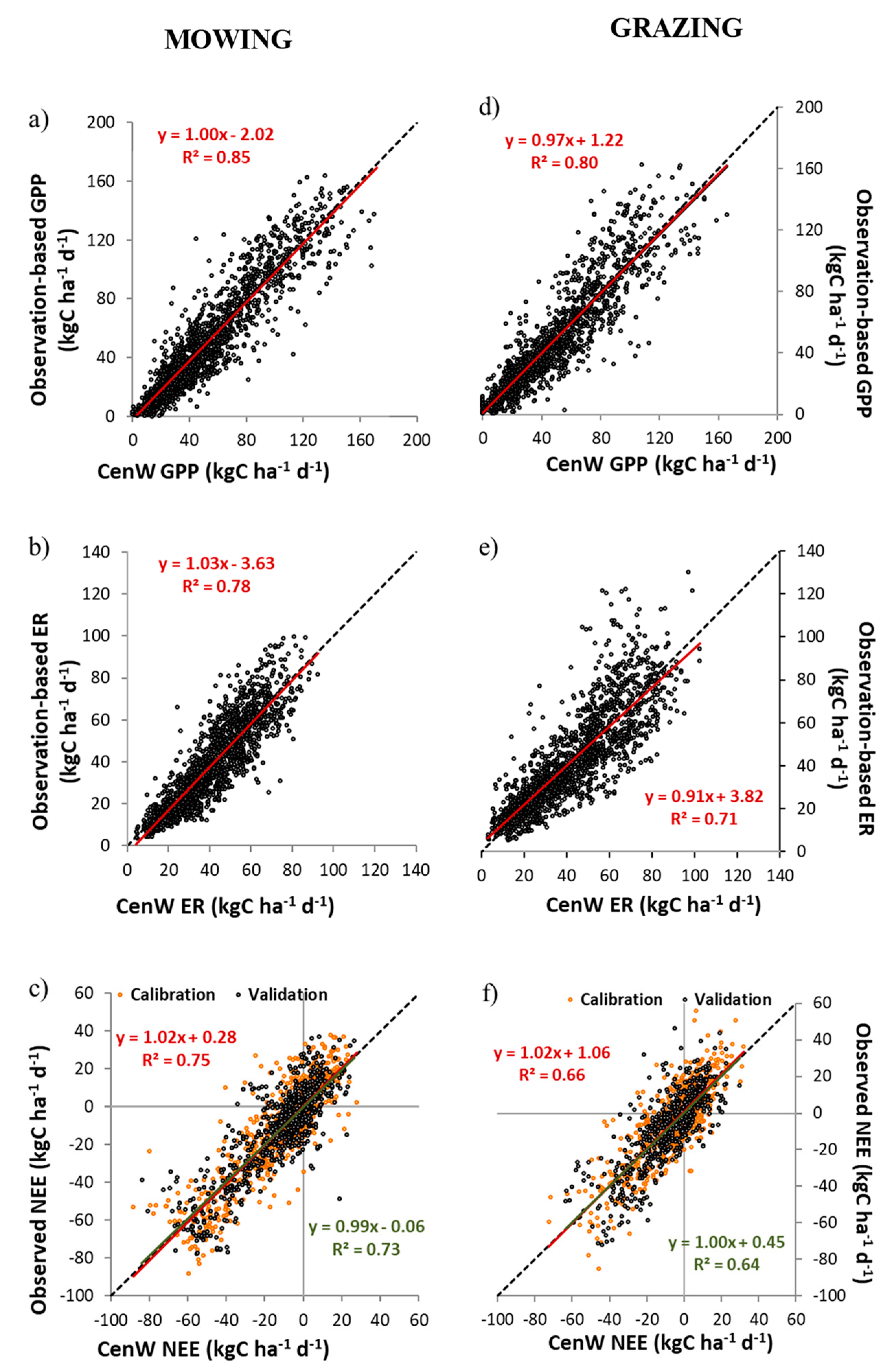
3.1.1. Carbon Dioxide Fluxes

Comparisons between modeled and measured daily CO2 fluxes for the two differently managed grasslands are shown in Figure 3, and model efficiencies for model calibration and validation are given in Table 1. In this section, only the best quality data from background periods (outside mowing and grazing events) were used for the comparisons. Observations that would have been affected by mowing and grazing events were omitted from the analyses [56], as well as days when fluxes from the eddy covariance systems had to be gap filled for more than 1/3 of half hourly periods. This selection of only best quality observation was necessary to avoid
  • the calibration of the model with data that strongly depended on another simpler model (i.e., the Reichstein gap-filling and partitioning tool) and
  • to limit the bias that would have resulted from the non or incomplete capture by EC of the large respiratory losses during measurement periods when grazing animals were present around the EC tower or when freshly cut or drying grass was present on the ground during mowing events [56,79].
For the NEE dataset, which was separated into parameterization and validation subsets, R2, and model efficiencies are slightly higher for the parameterization subset than for the validation one for the two grassland sites. Moreover, in general, model/data agreements (Figure 3 and Table 1) are better for GPP and ER than for NEE as it is easier to model large photosynthesis and respiration fluxes than the relatively small difference between the two (NEE). Model/data agreements are also better for mowing than for grazing, certainly because of the higher complexity of grazed systems compared to mowing. On the one hand, for the mowed paddock, management practices (mowing events and fertilizer applications) are accomplished within a day and evenly applied to the field. While, on the other hand, for the grazed paddock, grazing events last several consecutive days, the stocking density vary for the different events, there are dung and urine patches, there is an uneven reparation of cattle on the paddock, there could be some preferential grazing of plant species, and pasture could be damaged by trampling.
After parameterizing the model with good quality data over the full length of the study period (2006–2010), we obtained good agreement between modeled and observed carbon fluxes. Figure 3a,b shows the comparison of daily modeled GPP against their observation-based counterparts for the mowed and grazed paddocks, respectively. Good agreement was shown for both managed grasslands by the slopes close to 1, small intercepts of the linear regressions, and high correlation coefficients (R2 = 0.80–0.90). For the mowed paddock, model efficiencies for GPP were 0.86 and 0.88 for daily and weekly averaged fluxes, respectively (Table 1). Slightly lower, but still good EF was also found for GPP of the grazed paddock with daily and weekly model efficiencies of 0.80 and 0.79, respectively (Table 1).
The model also showed good performance in simulating daily and weekly averaged ecosystem respiration rates for both sites. For instance, the daily EF and R2 were 0.79 and 0.85 for the mowed and 0.73 and 0.71 for the grazed paddocks, respectively (Figure 3b,e). The grazed paddock had higher ER values than the mowed paddock and there was more scatter in the model/data comparison (Figure 3b,e) according to the lower values of R2 for daily and weekly comparisons.
The comparison of modeled NEE with EC measurements showed that the CenW model performed well in capturing the variability in NEE in background conditions. Across the two studied grassland sites, the CenW model explained between 65 and 74% of the variation in daily NEE for the mowed and grazed paddocks, respectively (Figure 3c,f and Table 1). For the mowed paddock, the coefficients of determination for daily and weekly averaged net carbon fluxes were 0.74 and 0.77, respectively (Table 1). The agreement between observed and modeled NEE for the grazed paddock was lower than for the mown paddock with daily and weekly R2 of 0.65 and 0.71, respectively. For the two managed grasslands, the overall seasonal and annual variations in NEE are reasonably well modeled and consistent agreement between modeled and measured NEE was achieved with daily model efficiencies of 0.74 and 0.65 for the mowed and grazed paddocks, respectively.

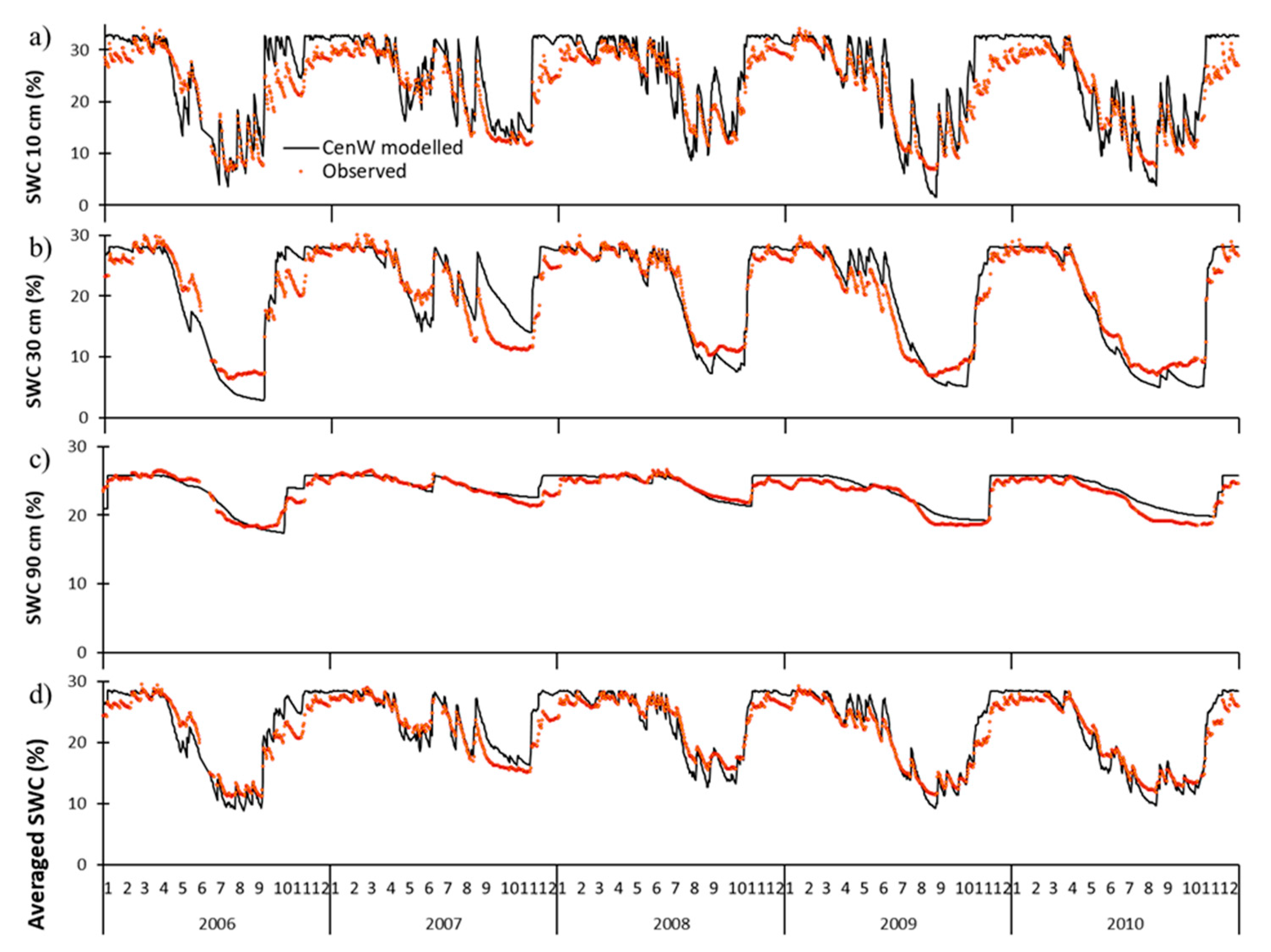
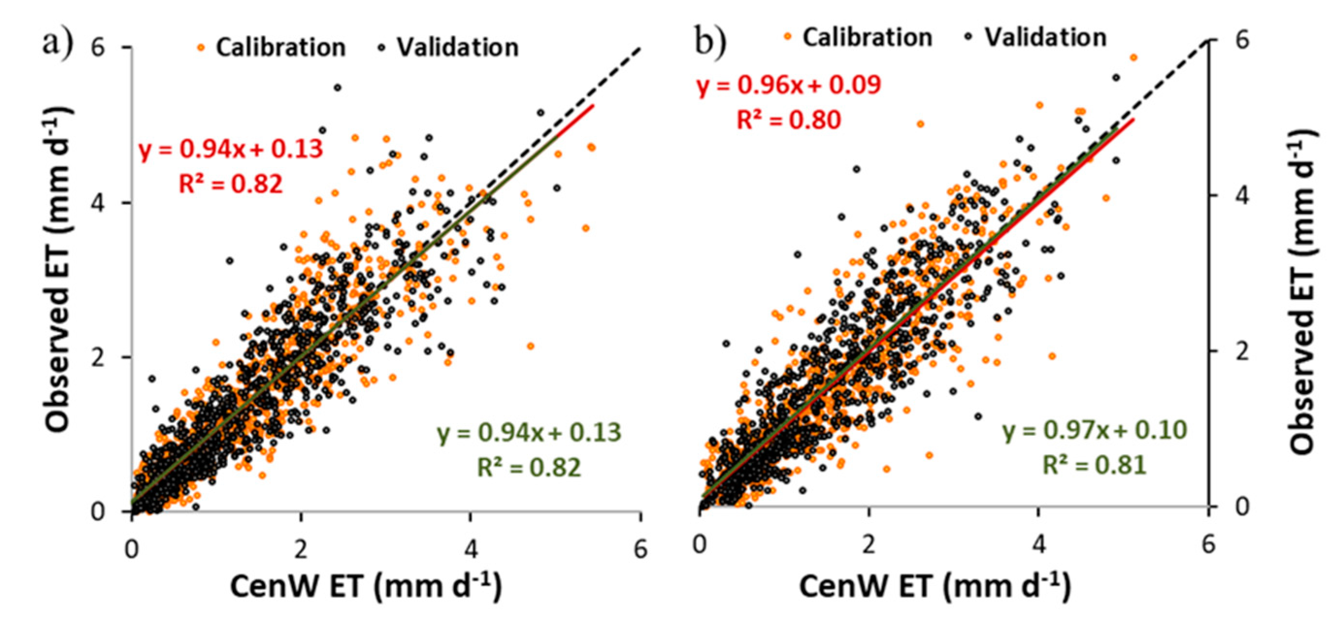
3.1.2. Soil Water Content and Evapotranspiration

Evapotranspiration (ET) measurements were also used for the parameterization and validation of the CenW model for both grassland sites. Soil water content observations were only available for the mowed paddock and were not used for the calibration of the model. Figure 4 shows the time series of daily observed and modeled soil water content (SWC) of the mowed paddock for three depths averaged over the entire soil profile.
Over the entire study period, the soil water content measured and modeled at different depth agree quite well (Figure 4a–c), confirming the correct set up of the soil water flows procedure in CenW. Averaged soil water content was generally well modeled, with an EF of 0.83. On average, over the study period and over the entire soil profile, modeled and measured SWC were 22.4% and 21.9%, respectively.
There was no systematic over- or underestimates of soil water content. Lower modeled SWC were found in spring 2006 and during summers of 2008 and 2010 (Figure 4) and were most likely due to higher CenW modeled water losses in spring and early summer than actual field conditions. Conversely, measured SWC was sometimes lower than modeled values. In 2007, observed soil water drawdown was faster than model simulation, but Figure 6d shows no discrepancies in ET, and so the problem seems to be linked to water drawdown. It could be that CenW extracted too much water from deeper layers and preserved it in the top layers. This situation was encountered following a water-limited period and could be due to cracks in the soil, causing preferential water flows not accounted for in the model or to the incomplete capture of vegetation dynamic in response to droughts.
Overall agreement for SWC is good, and remaining discrepancies could be due to measurement errors like the heavy rainfall in 2006 either not measured correctly, or not all water infiltrating but running off. Others could be due to shortcomings of the model, like not having soil cracks represented, or because of some measurement uncertainties reducing the model/data agreement. Because SWC and ET are tightly linked, achieving to get a good agreement between observed and modeled soil moisture is consistent with the good results reported for the modeling of daily and weekly evapotranspiration rates (Figure 5a and Table 1).
The CenW model explained more than 80% of the variation in daily ET for the two grassland sites. There was a close agreement between modeled and observed daily ET across the monitoring period (Figure 5), with R2 of 0.82 and 0.81 and EF of 0.82 and 0.80 for mowed and grazed paddocks, respectively. The coefficients of the linear regression lines (Figure 5) show a tendency of the model to slightly underestimate low ET (positive intercepts) and overestimate high evapotranspiration rates (slopes lower than 1), however slopes and intercepts are very close to their optimal values, showing that there is no systematic differences between modeled and observed evapotranspiration rates.
Overall, very good agreements between the CenW modeled and observed daily CO2 and water fluxes were achieved for both management practices (i.e., mowing and grazing). This indicated that the response of the model to climatic conditions and management practices were well captured in the simulations and that most of the processes encountered in the fields were properly implemented in CenW. Student’s t-tests were used to statistically test if slopes of linear regressions were significantly different from 1 and intercepts different than 0. Results showed that for water and all carbon fluxes, except NEE, for the two grasslands management, the slopes and intercepts were significant (p-values < 0.05). Even though GPP and ER were not used to parameterize CenW, there was nonetheless very good agreement between simulations and measurements (Figure 3a–d and Table 1). This indicate a high correlation between photosynthesis and ecosystem respiration rates derived from NEE data according to the Reichstein partitioning algorithm and fluxes modeled by the mechanistic CenW model.

3.2. Seasonal and Interannual Variabilities of Modeled and Observed Carbon Dioxide and Water Fluxes

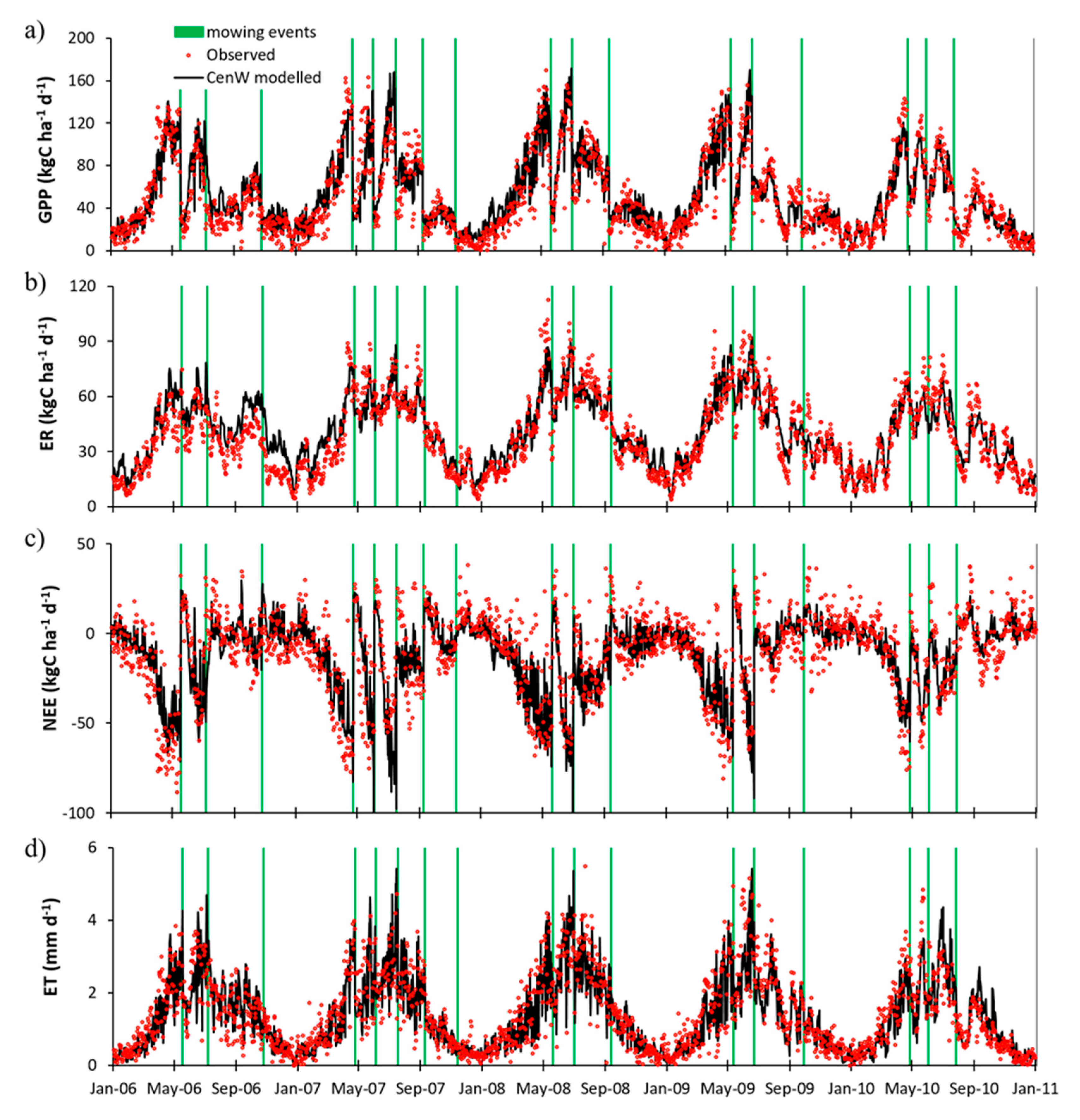
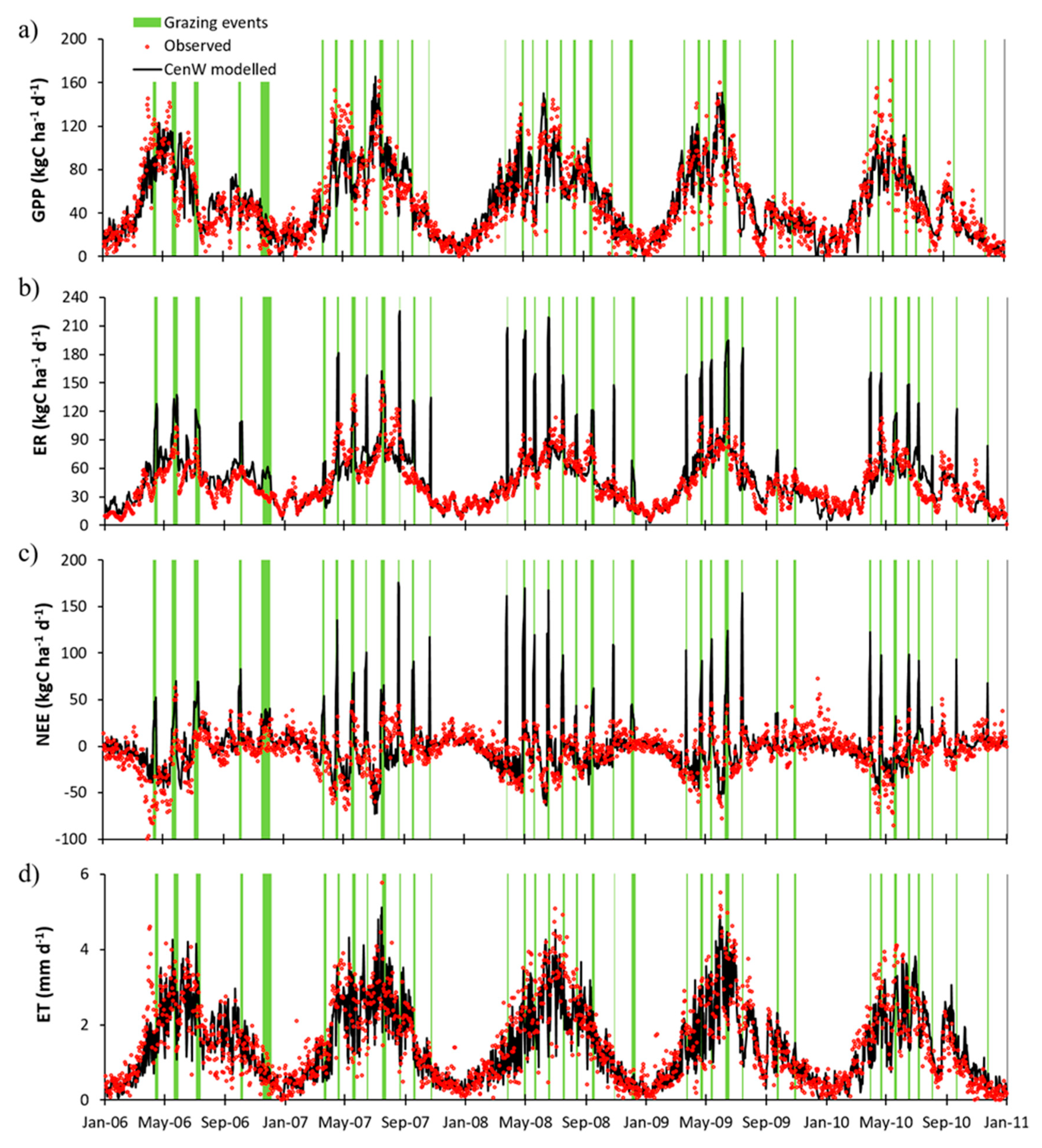
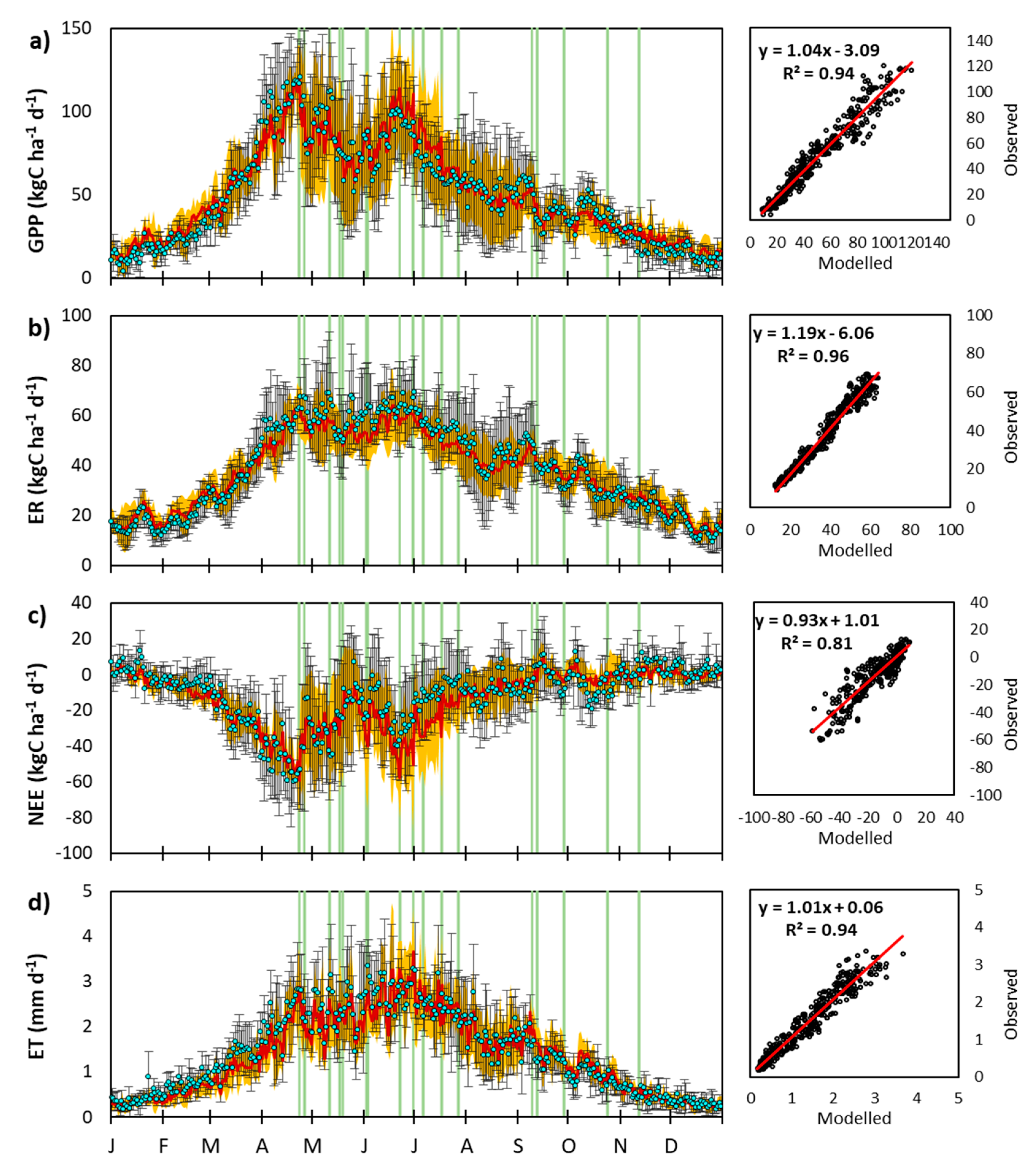
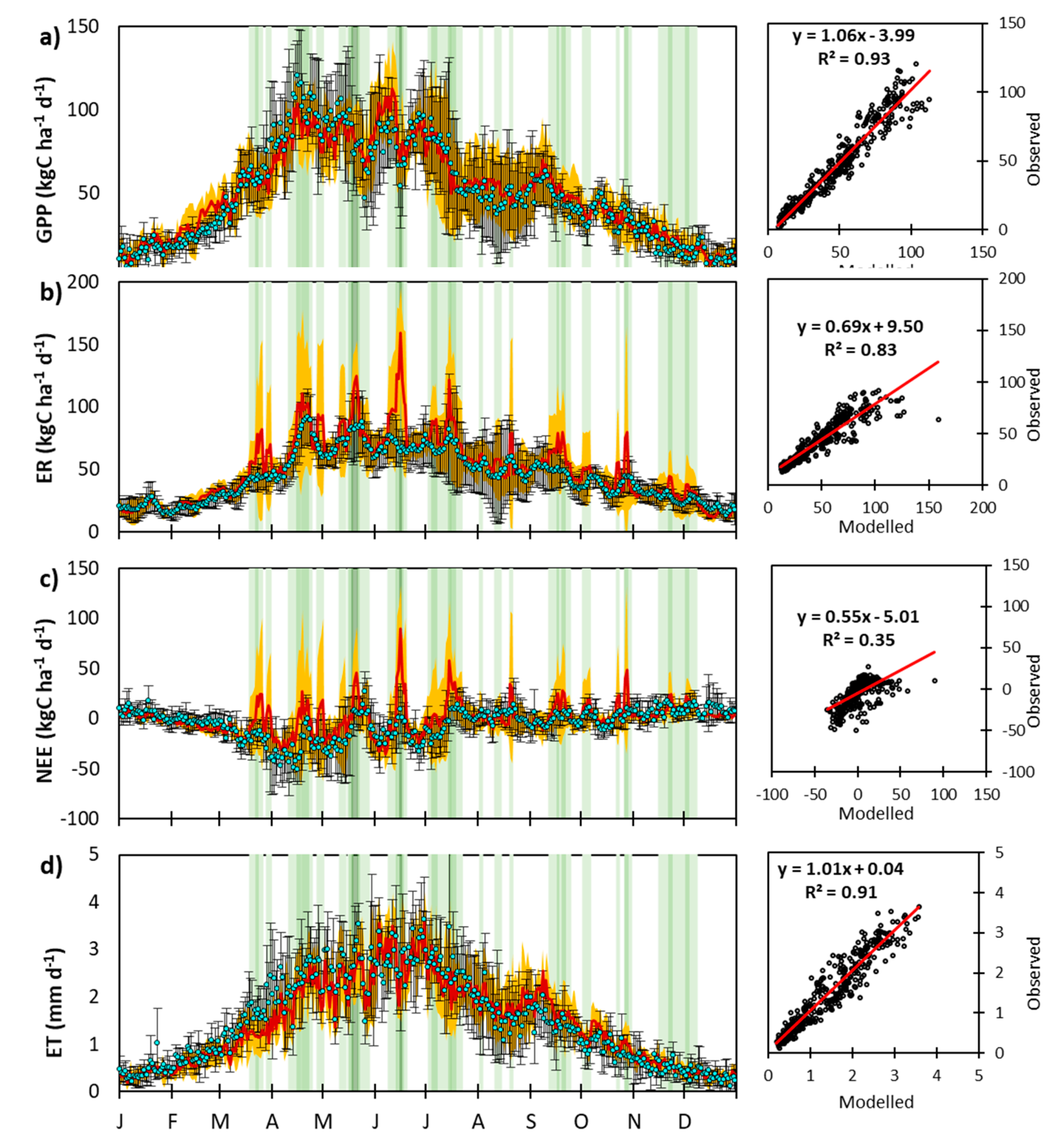
3.2.1. Day-to-Day and Seasonal CO2 and Water Fluxes Variability

For managed grassland ecosystems, important drivers of day-to-day and seasonal variabilities are management practices, particularly the timing and intensity of mowing and grazing that combine with the natural temporal climate variability to drive the behavior of ecosystems and strongly affect the CO2 dynamic and C balance of managed grasslands [8].
Depending on a number of climatic factors (solar radiation, temperature, and precipitation), ecological factors (leaf area and water, nutrient, and temperature stresses), and management practices (nitrogen fertilization, mowing and grazing timing, duration, and intensity), modeled and observed CO2 and water fluxes demonstrate pronounced temporal dynamics over several years [79], as exemplified by the time series presented in Figure 6 and Figure 7.
The apparent day-to-day and seasonal variabilities of observation based GPP was well captured by the CenW model for both of the managed grassland sites (Figure 6a and Figure 7a). The highest assimilation rates occurred during spring and summer, with GPP values up to 160 kgC ha−1 d−1 when growth conditions were the most favorable. Over the summer months, both modeled and observed GPP were reduced through water limitations, which occurred over most summer months but varied in intensity from year to year. Lower CO2 assimilations rates were found during the winter months as temperature and radiation were low and limited photosynthesis and vegetation growth, but some gas exchange continued throughout even the coldest winters. After mowing events, during the peak growing season, GPP was strongly reduced down to wintertime levels. GPP typically dropped from preharvest values in the range of 120 to 160 kgC ha−1 d−1 to postharvest values between 20 and 50 kg C ha−1 d−1 (Figure 6a and Figure 7a). These reductions of GPP by 2/3 are important and even if, on average, only three harvests were carried out each year, they have significant and long-lasting effects on ecosystem behavior and gas exchange. CenW managed to simulate accurately the recovery of the ecosystem gas exchanges rates (Figure 6, Figure 7, and Figure A1) after cutting and grazing events.
The day-to-day variability of observation-derived ER was also reasonably well captured in the model simulation and the seasonal pattern was well reproduced, in particular, displaying ongoing reasonably high respiration rates throughout the winter months (Figure 6b). Harvesting did not affect ER as strongly as GPP (Figure 6a,b) since autotrophic respiration from above ground vegetation is only part of the total ecosystem respiration, and (belowground) heterotrophic respiration was mostly unaffected by harvests. Because NEE is the difference between the two large fluxes of C assimilation through photosynthesis (GPP) and ecosystem respiration (ER), it was also affected by vegetation harvests (Figure 6c).
Mowing changed the pasture CO2 status from a net carbon sink to a net source, and it usually took a few days to a week for NEE to become a sink again, and a few more weeks to return to preharvests carbon fixation levels. On average, over the five years of the study, the GPP recovery from mowing took 20 to 25 days. The seasonal and day-to-day variability of GPP and ER, controlled by the variability of climate conditions and timing of harvests causing the sharp reduction of photosynthesizing and respiring biomass, were well captured by the CenW model for the mowed grassland area.
Evapotranspiration flux (ET) was highest during spring and summer when climatic conditions were the most favorable for water losses and vegetation was the most active (Figure 6d). The removal of aboveground biomass by harvesting or grazing led to sharp reductions of the transpiration rates, partially compensated by the increase in soil transpiration caused by an increase of solar radiation reaching—and higher temperature at—the soil surface.
Grazing events greatly affected GPP and ET (Figure 7a,d) and caused massive spikes in modeled ER due to cattle respiration (Figure 7b). Similarly to the mowed paddock discussed above, the removal of photosynthesizing biomass by grazing animal caused an important subsequent reduction in carbon assimilation rates (GPP). However, in contrast to harvest events which were sudden and restricted to single days, the removal of biomass by dairy cows was progressive and spread over several consecutive days (on average five days). GPP reductions were therefore not as abrupt as for the mowed grassland (Figure 6a, Figure 7a and Figure A1) and generally, postgrazing daily modeled and observed GPP values agreed well and remained higher than postharvest values, which most likely resulted from the extent of biomass removal that differ between the two treatments.
Day to day variability and seasonality of ER and NEE of the grazed paddock were also reasonably well captured by CenW (Figure 7b,c), but there were large discrepancies between these two daily modeled and observed variables during most of the grazing events. These differences resulted from the fact that the CenW model specifically simulated grazers’ respiration rates based on measured amounts of vegetation ingested, which caused the large pulses in modeled ER and NEE. According to CenW simulations, the grazing animal respiration rate is 4.15 kg C head−1 d−1 (4 µmol CO2 head−1 s−1). In some cases, such pulses were visible but much smaller in the eddy covariance measurements than in the model. Measurements could only record what happened within the flux footprint, which varied with wind speed and direction while the CenW model simulated the whole paddock. If all dairy cows were not inside the footprint at any given time, it would have been impossible for the EC tower to measure total grazing animals’ respiration while it was fully accounted for in the CenW model. At other times, a large number of cows might have been present within the flux footprint and their respiration would have been captured by the EC system. However, because this rate could have been an order of magnitude higher than the base respiratory carbon flux from the soil and pasture [56] the corresponding data could have been filtered out during the processing of EC fluxes. If the resultant data gaps during grazing events were filled using the traditional Reichstein gap-filling and partitioning algorithms it could have resulted in gaps being filled based on data collected during periods in the preceding and following week when there were no cows present within the flux footprint.

3.2.2. Interannual Variability of CenW Modeled and EC Measurements of CO2 and H2O Fluxes

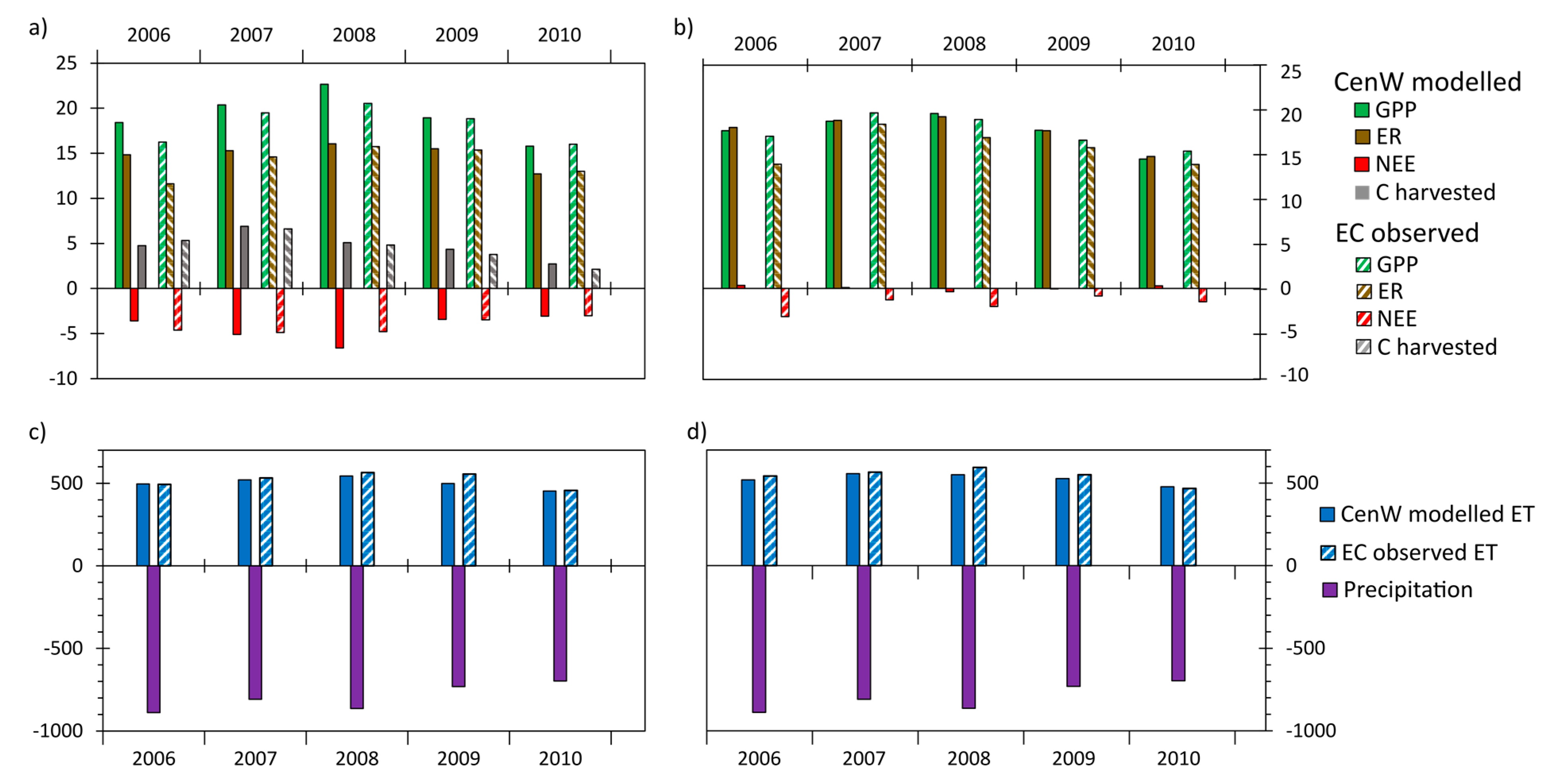
Interannual Variations in Mean Daily Fluxes

Generally, daily modeled and observed fluxes averaged over the five years of the study agreed very well for the mowed grassland site, as well as their interannual variations (+/– 1 SE from the 5-year daily averages). This is highlighted in Figure 8 by error bars (for EC observed fluxes) and yellow area (for CenW modeled fluxes) and confirms that the CenW model simulations captured well the fluxes variations due to differences in meteorological conditions and management for the mowed paddock.
Higher interannual variability was found during the most productive seasons (spring and summer), in which most of the harvest events occurred (on different days each year). GPP is more variable than ER because of the larger direct impact of harvest on photosynthesizing biomass that on total ER. Water limiting conditions and the onset of harvest events (end of April–early May) led to a substantial reduction of GPP and hence of the net ecosystem exchange rate with NEE averaged values during this period as low as wintertime fluxes.
For the grazed paddock, modeled and observed daily averages (over five years) agree very well for GPP (Figure 9a), as well as their interannual variability (error bars), confirming that the main biotic and abiotic factors controlling the dynamic of GPP were properly incorporated in the CenW ecosystem model. Weaker correlations were found between observed and modeled ER (Figure 9b) and NEE (Figure 9c) during grazing events while outside of grazing periods good agreements were retrieved. These large differences were likely caused by the noncapture of some or all of grazing animals’ respiration by the EC system.
Overall, model/data agreements are greatly variable and strongly depend of climate conditions and management practices (Figure 8 and Figure 9).

Variability of Annual CO2 and Water Fluxes

Correlations between climate, management practices and CO2 and water fluxes are showed through a matrix plot (Figure 10). The different categories correspond to modeled and observed variables for the mowed and grazed paddocks. All points represent one year of either modeled or observed variables for the two sites summed/averaged over the summer half-year (15 April to 15 September), corresponding to the most productive time of the year. Lower panels show the scatter plots between the different selected variables and the upper panels give their correlation coefficients. For example, the pink-circled lower panel show the scatter plot of NEE and precipitation and the pink-circled upper panel give the corresponding correlation coefficients for the different categories (MG, MM, OG, and OM) and the overall correlation coefficient (Cor). The blue-circled area of the graph shows the selection of the most important relationships.
First, it is striking (Figure 10) that annual CO2 and H2O fluxes were correlated with annual meteorological condition (air temperature and precipitation) and with management practices (C harvested/grazed and N fertilizer applications) but with marked differences across the two managed grassland sites.
For the mowed paddock, observed, and modeled amounts of carbon harvested are highly correlated with air temperature (OM: −0.78 and MM: −0.93), precipitation (OM and MM: 0.82), and N fertilizer (OM: 0.93 and MM: 0.99). On the contrary, correlations for the grazed paddock were lowest with N fertilizer (OG: 0.57 and MG: 0.60) and weak with climate (|OG| and |MG| <0.50).
The analysis also showed that, for the mowed paddock, the modeled and observed NEE were highly correlated with climate and management practices, but that for the grazed paddock NEE values were only weekly correlated with other variables. In this section and like for all this study, negative NEE represent a net gain, and a positive NEE is a net loss of CO2 for the ecosystem. It is interesting that for the grazed paddock, modeled, and observed summer half-year NEE responded differently to the amount of vegetation grazed (i.e., CenW giving a positive moderate correlation of NEE with the amount of vegetation grazed while observations were giving a week negative correlation). This is due to the differences between modeled and observation-derived ER rates during grazing events and CenW simulating higher ER rates during grazing events: the more vegetation is eaten the more NEE increased (reduction of the sink strength of the pasture).
There were also high correlations between ET, climate and management practices for both grasslands, with a general upward trend of ET as precipitation, amounts of N fertilizer and C mowed/grazed increased and a downward trend with the increase of air temperature. More water vapor is returned to the atmosphere when there was more rainfall compared to dryer and hotter spring and summer periods.
The modeled and observed annual (full year average/sum) carbon and water balances for the mowed and grazed paddocks are shown in Figure 11. For the mowed paddock, observed annual GPP values ranged between 16 and 20.5 tC ha−1 yr−1 (five-year average: 18.2 tC ha−1 yr−1) and modeled GPP values ranged between 15.3 and 22.7 tC ha−1 yr−1 (five-year average: 19.2 tC ha−1 yr−1). For the grazed paddock, observed annual GPP values ranged between 15.9 and 20.3 tC ha−1 yr−1 (five-year average: 18.1 tC ha−1 yr−1) and modeled GPP values ranged between 14.9 and 20.2 tC ha−1 yr−1 (five-year average: 18.2 tC ha−1 yr−1).
On all years but 2006, CenW-modeled ER for the mowed paddock were lower than annual sums of EC-derived ER (Figure 11) with annual modeled ER values between 12.7 and 16.1 tC ha−1 yr−1 (five-year average: 14.9 tC ha−1 yr−1), while observation-based ER values varied from 11.6 to 15.7 tC ha−1 yr−1 (five-year average: 14.1 tC ha−1 yr−1). For the grazed paddock, model/data differences were even more important with annual EC-derived and modeled ER varying from 14.3 to 19.0 tC ha−1 yr−1 (five-year average: 16.3 tC ha−1 yr−1) and from 15.2 to 19.9 tC ha−1 yr−1 (five-year average: 18.3 tC ha−1 yr−1), respectively.
There is a good agreement between modeled and observed annual amounts of harvested C. Generally, the modeled and observed annual NEE agreed reasonably well for the mowed grassland sites but large differences were retrieved for the grazed paddock and might result from the miss or only partial capture of grazing animals’ respiratory losses by the EC system. Five-year averages of observed NEE for the mowed and grazed grassland sites were −4.2 (−3.0 to −4.9) and −1.8 (−0.9 to −3.2) tC ha−1 yr−1, respectively. CenW modeled NEE, averaged over 5 years, were −4.4 (−3.1 to −6.6) tC ha−1 yr−1 for the mowed paddock and 0.1 (−0.4 to 0.4) tC ha−1 yr−1 for the grazed pasture. Modeled annual net CO2 fluxes, for the grazed paddock, were significantly lower than observed ones because, as we have seen, part of C harvested (grazed) is taken into account in observed NEE, while it is fully accounted for in the modeled NEE. Apparently, the mowed paddock fixed more CO2 than the grazed paddock however, when harvested C is taken into account (Figure 11a) the mowed grassland C sink activity is drastically reduced.
Modeled and observed daily evapotranspiration rates generally agreed very well as we have seen in Section 3.1.2 with EF of 0.82 and 0.80 for the mowed and grazed paddocks, respectively. Both modeled and observed summer half-year evapotranspiration rates were higher for the grazed paddock because of the differences management practices (harvests and grazing) that affected vegetation dynamics. Even if there were fewer harvests than grazing events, the dramatic reduction of live foliage following grass cuttings affected water fluxes and reduced the annual amounts of evapotranspiration. Modeled summer half-year ET were also systematically lower than the observed results, which could result from (1) differences in modeled and observed roots dynamics (growth and senescence) affecting soil water extraction by plants and (2) the water returned directly to the field by cattle urinations which is not accounted for in the model. Observed five-year average annual ET were 521 and 544 mm yr−1 while modeled values were 503 to 527 mm yr−1 for the mowed and grazed paddocks, respectively.
It also as to be noted that the conventional gap-filling and partitioning tool [69] was not designed to deal neither with heterogeneities in ecosystems as it the case in intensively managed grasslands, like our study site, nor to take into account the varying magnitude of respiratory CO2 losses from rotationally grazing animals that not depend of meteorological conditions. These conditions would add uncertainties in gap filled NEE fluxes and on their partitioning into GPP and ER [79].

4. Discussion

4.1. Performances of the CenW Model to Simulate Gas Exchanges of Mowed and Grazed Pastures

Mechanistic ecosystem models, like the CenW model, are useful tools to gain a better understanding of GHG emissions, yields, and carbon stock dynamics of managed grasslands as they can address, over long time periods, the complex interactions between climate, soil, vegetation and management practices [80,81,82]. Modeling studies have shown that models could achieve high accuracy in simulating greenhouse gas (CO2 and H2O) uptakes and emissions, yields, and carbon source/sink activity of managed grasslands for a wide range of climate and management conditions [17,56,83,84,85,86].
By using observation and models in conjunction, it is possible to improve our knowledge of the systems under study, identify weaknesses in datasets and models and to correct them. Over the study period, the site experienced large variations in temperature, moisture availability, and radiation, which are controlling factors of the exchange rates between the atmosphere and grasslands of CO2 [87,88,89,90] and water fluxes [91]. In addition, grazing and cutting dramatically alter the way managed grassland ecosystems respond to climate drivers by the sharp removal of large amounts of live biomass [36,92,93] and thus strongly affect the seasonal and inter-annual variabilities of gas exchanges and the annual carbon budgets of the farm/paddock [22,79,94].
Modeling NEE accurately is generally difficult as NEE is calculated from the (relatively small) difference between the two largest carbon fluxes between the atmosphere and the ecosystem (vegetation + soil), i.e., GPP, which is the carbon gain through photosynthetic CO2 assimilation and ER, which corresponds to total ecosystem respiratory losses by plant autotrophic, soil heterotrophic and also by grazing animals’. Accurate and reliable modeling of daily NEE fluxes requires that the CenW model properly incorporates and simulates the main processes driving the dynamics of both ecosystems (mowed and grazed grasslands). This study aimed to confirm the applicability of the CenW ecosystem model to simulate managed grassland systems.
Generally, better agreements between observed and modeled NEE and its components GPP and ER were found for the mowed paddock than for the grazed one. This could be because there were more frequent, longer and more spatially heterogeneous disturbances on the grazed than on the mowed paddock. In addition, uncertainties in the amounts of vegetation removal and respiration rates of grazing animals likely reduced the overall agreement between CenW outputs versus observations for the grazed paddock. Over the entire study period and for the two managed grasslands, CenW tends to slightly overestimate the lowest rates of C assimilation (Figure 3a,d) and ecosystem respiration (Figure 3b,e) and to underestimate large values of both uptake and emission of C fluxes as indicated by the slopes and intercepts of the linear regressions. After the careful parameterization of the CenW ecosystem model, very good agreements were found between simulated and observed carbon and water fluxes, highlighting that the model, parameterized with local data could appropriately be applied to intensively managed grasslands, as long as sufficient information on management practices are available.

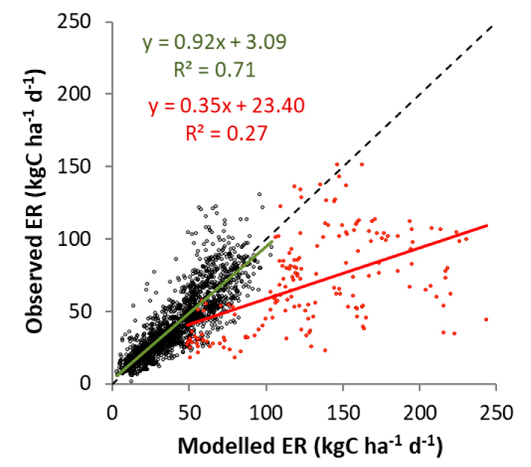
4.2. Cow Respiration in Observed and Modeled CO2 Fluxes

Discrepancies between modeled and observed ER and NEE fluxes, on the grazed paddock, could be caused by the uneven repartition of dairy cows on the field and the variability of the flux footprint: i.e. dairy cows were under-represented in the flux footprint, causing an under-estimation of animal respiratory losses of CO2 in EC data. Some large grazer respiration fluxes could have also been excluded through the filtering of NEE data to remove outliers (condition 1, 2 and 3 in Section 2.1.2). Moreover, because the Reichstein gap-filling algorithm does not explicitly include respiration from grazing animals (e.g., animals disturbance) to either fill gaps in NEE time series or in the partitioning of NEE into GPP and ER, substantial bias could be added to the dataset [56,79]. For all measurements without grazing there was good agreement between the CenW model and EC observations, highlighting the correct parameterization of the model and confirming that most of the ecosystem processes were well embedded in the model. It also showed that large discrepancies were present during grazing periods because of the possible non or only partial capture of cows respiration in NEE data (Figure 7c, Figure 9c and Figure A1).
A recent EC study of CO2 fluxes on two paired sites under rotational and continuous grazing management, found that ER for the rotationally grazed paddock was greatly affected by cattle respiration and that grazing animal’s respiration was correctly accounted for in EC measurements [95]. In this study, we showed that there is, during grazing events, a possible underestimation of observation-derived ER from the EC system placed on the grazed paddock (Figure 12), which is consistent with other studies on managed grassland that found no effect of animals’ respiration on EC-derived ER [92,93,96]. By comparing daily EC-derived ER with their CenW modeled counterparts (Figure 12), we showed that, on a few cases (red dots around the one to one line), modeled and observation-derived ER agree very well, showing that cattle respiration was properly modeled and measured by the flux tower. However, for most of the grazing events recorded, a large proportion or all of cattle respiration was not captured by EC (red dots strongly deviating from the one to one line). This was likely caused by the uneven spatial repartition of animals on the paddock, shifts in flux footprint, specific site conditions, stocking densities, and the processing of EC data [75,93].
In this study, we showed that the direct effect of grazing (i.e., the reduction of photosynthesizing biomass [22]) was properly captured in EC data but that the indirect effect (i.e., grazing animals’ respiration [22]) was not captured by EC systems because of the stochastic position of cows and shifts in the flux footprint area. To fully understand why grazers’ respiration is not accounted for and to find a way to correct EC data for this bias, using a biochemical, process-based ecosystem model incorporating management practices, like CenW, alongside dairy cows positioning devices and detailed flux footprint information, could be necessary [79,94].
Another problem is also related to the gap-filling process since algorithm used for this task did not use any information on cows’ position and their respiration rates. If actual data affected by the presence of cows in the footprint were used to fill gaps outside of grazing periods, the large (depending of the number of cows) respiration would bias gap filled fluxes [79].
We advocate that a better way to process EC data on rotationally grazed pasture would be to exclude measurements taken during grazing periods and fill the gaps outside and inside these periods with data acquired when there was no cows in the paddocks [97]. This would insure to get the flux from the pasture only [79,94], and then calculate how much carbon is lost from the paddock due to grazers respiration based on stocking rates, grazing duration, and amount of ingested biomass. This imply that detailed information on cows movement and farming practices need to be recorded and used to process EC data from intensively manage grasslands, especially for systems with high stocking rates like rotational grazing.
The same dataset (we reprocessed meteorological and EC data for this study) was previously used to derive the net carbon storage (NCS) of the mowed and grazed grasslands [26]. They found that the grazed grassland have the potential to sequester more C than the mowed grassland but this implied that cows’ respiration was accurately enough measured by EC. However, we showed by applying the CenW model that important respiratory losses (from grazing animals) were not accounted for in eddy covariance measurements taken on a intensively, rotationally grazed grassland (Figure 12). We showed that measured and modeled NEE fluxes agreed very well outside of grazing periods but strongly deviated during grazing events due to the noncapture of cows respiration by the EC system. CenW modeled annual NEE values (Figure 7c and Figure A1) were found to be almost 10 times lower than the annual NEE values from EC data. As a result, the carbon storage capacity of this grazed grassland site would have been strongly reduced if cows respiration was adequately captured by the eddy covariance system.

4.3. Seasonal Variability of Observed and Modeled CO2 and Water Fluxes

The natural variability of carbon and water fluxes, caused by short (day to day) and long term (seasonal) variations in climate conditions, management and vegetation dynamics is well captured in model runs. It is notable from time series (Figure 6, Figure 7, Figure 8 and Figure 9) that grazing caused a greater interannual variability than mowing in all three carbon fluxes (i.e., GPP, ER, and NEE).
Unlike natural ecosystems, in intensively managed grasslands, the seasonal and interannual variability of carbon and water fluxes not only depends on the variability of the governing climate variables, but also on farming practices [36,98,99,100]. This is mostly a result of the rapid and sharp reduction of photosynthetically active biomass caused by mowing and grazing events that reduce GPP and switches the system from being a sink to a source of CO2 [32,93,100]. However, because of the regular N fertilizer applications, and unlike for natural ecosystems, the N limitation is almost suppressed, promoting the rapid restart of GPP and vegetation growth.
Measured eddy covariance data showed a larger temporal variability than the modeled signals (Figure 8 and Figure 9). This could be explained by the fact that EC data measurements contain random errors that add up to the “real” flux and that scale with the magnitude of the fluxes and hence vary diurnally and seasonally [101]. Therefore, this random error term could lead to an under or overestimation of the measured fluxes. Whereas CenW is always in the middle, where rates ought to be and the scatter in both directions cancelled out. It is also possible that these higher rates than the average are not artifacts and that the formalism of the model not allow to simulate these fluxes because we either do not know which processes are causing them or something not recorded happened on the farm. In the mowed paddock, ER was less affected by mowing events than GPP because only the autotrophic respiration of plant leaves term was affected by the sharp reduction of live foliage [88,95].
Seasonal dynamics of the soil moisture profile were controlled by temporal distributions of water gain from precipitation and ET losses, which were well captured by the model (for the mowed paddock). Soil water content observation and CenW showed larger variations in shallow soil layer than deeper in the soil profile and generally agree reasonably well.

5. Summary and Conclusions

This study investigated the performances of the CenW ecosystem model to simulate carbon and water fluxes from paired eddy covariance towers of two managed grassland systems in France with different management practices: mowing vs grazing. It showed that once parameterized, model/data agreement was very good for both sites and that CenW could adequately reproduce flux variability in response to management and climatic condition at daily, seasonal and interannual time scales. Model efficiencies for daily CO2 fluxes were 0.65–0.80 and 0.73–0.85 for grazed and mowed paddocks, respectively. The mowed grassland ET, averaged SWC and harvested biomass were modeled with efficiencies of 0.82, 0.85, and 0.80, respectively. For the grazed paddock, model efficiency for daily ET was 0.80.
Our study showed that management practices highly determined the temporal dynamics and seasonal and interannual variabilities of CO2 fluxes and the C status of the grazed pasture. In addition, most of previous studies which derived annual carbon budgets of managed pastures from EC measurements assumed or showed that grazing animal’ respiratory losses were satisfactorily captured in NEE fluxes at annual time scales but showed weaknesses at smaller time scales [22,79].
It also highlighted that large discrepancies existed between measured and modeled net carbon exchange and ecosystem respiration rates during grazing events and that it is likely that large losses of CO2 to the atmosphere were not fully captured by the eddy covariance system. The model/data comparison showed that flux processing and interpretation needed to be done carefully in grazed systems to account for the presence of dairy cows in the paddock. So far, only few studies have used eddy covariance measurement in combination with process-based models in grazed pastures. Here our results clearly demonstrate that grazing animals’ respiratory flux is most often not captured by EC systems, which could lead to substantial bias in NEE data taken during grazing events.
In addition, because of the importance of CO2 losses of carbon not accounted for in the annual C budget, large overestimations of the C status of the farm are likely to be made.
The capture or not by EC of cows respiration is site specific, using detailed ecosystem models incorporating farming practices and their effects on vegetation and C dynamics could help to identify and correct possible issues with EC data in intensively managed grasslands. Model/data agreements for the mowed paddock were higher than those obtained for the grazed paddock, certainly because mowed systems are less complex and disturbed than grazed ones.

Author Contributions

Conceptualization, A.C., N.P., and N.S.; Methodology, N.P., A.C., and M.K.; Software, M.K.; Validation, N.P., A.C., and M.K.; Formal Analysis, N.P.; Investigation, N.P. and A.C.; Resources, A.C.; Writing—Original Draft Preparation, N.P.; Writing—Review and Editing, A.C., N.S., C.F., K.K., M.K.; Supervision, A.C.; Project Administration, A.C.; Funding Acquisition, A.C.

Funding

The research leading to these results has received funding principally by the New Zealand Government to support the objectives of the “Livestock Research Group of the Global Research Alliance on Agricultural Greenhouse Gases under grants SOW12-GPLER-LCR-PM (Proposal ID 16949-15 LCR)”, “The AnaEE France (ANR-11-INBS-0001)”, “AllEnvi”, and “CNRS-INSU”.

Acknowledgments

We would like to thank the National Research Infrastructure “Agro-écosystèmes, Cycles Biogéochimique et Biodiversité” (ACBB) for their support in field experiment and the database. We are deeply indebted to Christophe de Berranger, Marie-Laure Decau and Nicolas Mascher for their substantial technical assistance. Last but not least we would like to thanks Dr. Gregory Starr (Department of Biological Sciences, University of Alabama, USA) for his technical support in refiltering the dataset.

Conflicts of Interest

The authors declare no conflict of interest.

Appendix A. Management Records

Table A1. Management records for grasslands under mowing and grazing for the period 2006–2010 at the SOERE-ACBB, Lusignan, France.
Mowed Paddock (P2)Grazed Paddock (P4)
YearDate of MowingDate of N Fertilizer ApplicationAmount (kgN ha−1)Starting Date of Grazing EventLength of Grazing Period (Day)Stocking Rate (Head ha1)Date of N Fertilizer ApplicationAmount (kgN ha−1)
200617-May26-Feb6011-Apr716.85-Apr30
6-Jun24-May6019-May1016.824-May30
24-Oct28-Sep503-Jul103.9
2-Oct4.517.1
16-Nov1812.9
200723-Apr22-Feb8019-Mar513.528-Mar50
5-Jun27-Apr6016-Apr421.319-Jun30
17-Jul12-Jun6016-May719.419-Sep30
10-Sep26-Jul6014-Jun316.120-Sep30
12-Nov19-Sep6015-Jul810.6
20-Sep6020-Aug211
17-Sep417.4
22-Oct219.7
200819-May29-Jan12025-Mar224.829-Jan30
30-Jun22-May9028-Apr422.922-May30
15-Sep15-Jul6019-May2.420.628-Jul60
17-Sep6016-Jun420.617-Sep50
15-Jul416.8
11-Aug3.415
12-Sep618.7
27-Oct222.3
1-Dec8.254.5
200911-May17-Feb11023-Mar225.217-Feb50
22-Jun19-May6020-Apr4.524.519-May60
28-Sep7-Oct6011-May3.524.5
9-Jun819
13-Jul2.512.9
21-Sep417
27-Oct419.5
201026-Apr16-Mar9029-Mar2.519.416-Mar60
2-Jun29-Apr7019-Apr3.519.429-Apr50
26-Jul8-Jun5017-May5.519
14-Jun3.519
5-Jul2.514.8
2-Aug216.5
20-Sep1.515.2
22-Nov1.512.6

Appendix B. CenW Model Calibrated Parameters

Table A2. Main model parameters values used to simulate mowed and grazed grasslands after CenW calibration.
Parameter DescriptionLusignan MowedLusignan GrazedUnits
StandMinimum foliage turn-over 0.0220.022yr−1
Fine-root turn-over 2.492.49yr−1
Low-light senescence limit 0.0560.08MJ m−2 d−1
Max daily low-light senescence 0.0150.017% d−1
Max drought foliage death rate 6.086.76% d−1
Drought death of roots relative to foliage 0.0620.066
Mycorrhizal uptake 0.010.01g kg−1 d−1
Soil water stress threshold (Wcrit) 0.600.60
Respiration ratio per unit N 0.180.44
beta parameter in T response of respiration 1.981.96
Temperature for maximum respiration 4747°C
Growth respiration 0.290.32
Time constant for acclimation response of respiration 364247d
Water-logging threshold (Llog) 0.9990.994
Water-logging sensitivity (sL) 8.37.33
Ratio of [N] in senescing and live foliage 0.990.99
Ratio of [N] in average foliage to leaves at the top 0.830.78
Biological N fixation 1.717.9gN kgC−1
Growth Km for carbon 0.971.8%
Growth Km for nitrogen 1.943.7%
Drop of standing dead leaves 2.112.11% d−1
Decomposability of standing dead relative to metabolic litter 0.70.7
photosynthesisSpecific leaf area 17.519.3m2 (kg DW)−1
Foliage albedo 6.776.75%
Transmissivity 1.571.56%
Loss as volatile organic carbon 00%
Threshold N concentrations (No) 6.335.76gN (kg DW)−1
Non-limiting N concentration (Nsat) 41.642.4gN (kg DW)−1
Light-saturated maximum photosynthetic rate (Amax) 45.747.2µmol m−2 s−1
Maximum quantum yield 0.060.06mol mol−1
Curvature in light response function 0.4120.412
Light extinction coefficient 0.860.86
Ball–Berry stomatal parameter (unstressed) bb110.111.9
Ball–Berry stomatal parameter (stressed) bb288
Minimum temperature for photosynthesis (Tn) -4.1-4.1°C
Lower optimum temperature for photosynthesis (Topt, lower) 25.825.8°C
Upper optimum temperature for photosynthesis (Topt, upper) 30.0630.06°C
Maximum temperature for photosynthesis (Tx) 38.838.8°C
Temperature damage sensitivity (sT) 0.040.04
Threshold for frost damage 0.190.19°C
allocationAllocation to reproductive organs NoneNone
Fine root: foliage target ratio (nitrogen-unstressed) 0.980.90
Fine root: foliage target ratio (nitrogen-stressed) 3.64.6
Used target-oriented dynamic root-shoot allocation YesYes
Fine root:foliage [N] ratio 0.820.82
decompositionRelative temperature dependence of heterotrophic respn 0.490.75
Foliar lignin concentration 11.912%
Root lignin concentration 14.614.6%
Organic matter transfer from surface to soil 9090% yr−1
Critical C:N ratio 8.038
Ratio of C:N ratios in structural and metabolic pools 4.834.09
Exponential term in lignin inhibition 55
Water stress sens. of decomp. relative to plant processes 0.681.03
Residual decomposition under dry conditions 0.050.05
Mineral N immobilized 5.325.38% d−1
siteAtmospheric N deposition 22kgN ha−1 yr−1
Volatilization fraction 10.110.1%
Leaching fraction 0.460.46
Litter water-holding capacity 22g gDW−1
Mulching effect of litter 2.82.8% tDW−1
Canopy aerodynamic resistance 8378.7s m−1
Canopy rainfall interception 0.0440.044mm LAI−1
Maximum rate of soil evaporation 1.551.25mm d−1

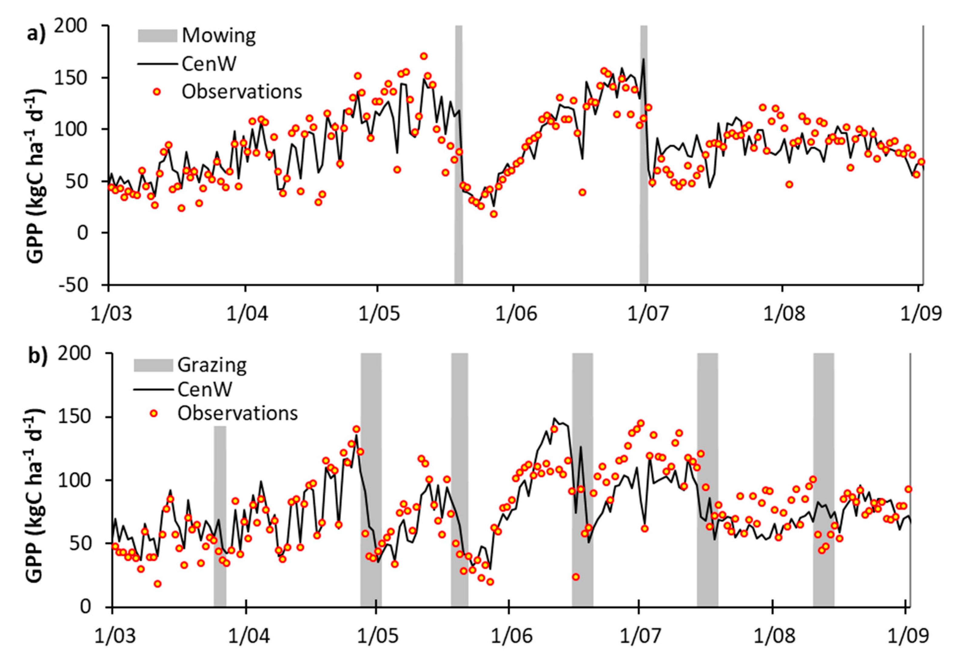
Appendix C. EC-Derived and Modeled GPP Time Series

Figure A1. Daily time series of EC derived (dots) and modeled (black line) GPP for a) the mowed and b) the grazed grassland sites over 6 months (March to end August) of 2008. Vertical gray areas represent the recorded timing of harvests and grazing events for the two selected paddocks.
Agronomy 09 00183 g0a1

References

  1. FAO and ITPS. Status of the World’s Soil Resources—Main Report; FAO and ITPS: Rome, Italy, 2015; ISBN 978-92-5-109004-6. [Google Scholar]
  2. FAOSTAT. Database Collection of the Food and Agriculture Organization of the United Nation. 2019. Available online: http://www.fao.org/faostat/en/#home (accessed on 4 January 2019).
  3. Scurlock, J.M.O.; Hall, D.O. The global carbon sink: A grassland perspective. Glob. Chang. Biol. 1998, 4, 229–233. [Google Scholar] [CrossRef]
  4. White, R.P.; Murray, S.; Rohweder, M. Pilot Analysis of Global Ecosystems: Grassland Ecosystems; World Resources Institute: Washington, DC, USA, 2000; ISBN 1-56973-461-5. [Google Scholar]
  5. Conant, R.T.; Paustian, K.; Elliott, E.T. Grassland management and conversion into grassland: Effects on soil carbon. Ecol. Appl. 2001, 11, 343–355. [Google Scholar] [CrossRef]
  6. Wang, W.; Fang, J. Soil respiration and human effects on global grasslands. Glob. Planet. Chang. 2009, 67, 20–28. [Google Scholar] [CrossRef]
  7. Herrero, M.; Henderson, B.; Havlík, P.; Thornton, P.K.; Conant, R.T.; Smith, P.; Wirsenius, S.; Hristov, A.N.; Gerber, P.; Gill, M.; et al. Greenhouse gas mitigation potentials in the livestock sector. Nat. Clim. Chang. 2016, 6, 452–461. [Google Scholar] [CrossRef]
  8. Soussana, J.F.; Allard, V.; Pilegaard, K.; Ambus, P.; Amman, C.; Campbell, C.; Ceschia, E.; Clifton-Brown, J.; Czobel, S.; Domingues, R.; et al. Full accounting of the greenhouse gas (CO2, N2O, CH4) budget of nine European grassland sites. Agric. Ecosyst. Environ. 2007, 121, 121–134. [Google Scholar] [CrossRef]
  9. Abberton, M.; Conant, R.; Batello, C. Grassland Carbon Sequestration: Management, Policy and Economics; Proceedings of the Workshop on the Role of Grassland Carbon Sequestration in the Mitigation of Climate Change; FAO: Rome, Italy, 2010; ISBN 978-92-5-106695-9. [Google Scholar]
  10. Reid, R.S.; Thornton, P.K.; McCrabb, G.J.; Kruska, R.L.; Atieno, F.; Jones, P.G. Is it possible to mitigate greenhouse gas emissions in pastoral ecosystems of the tropics? Environ. Dev. Sustain. 2004, 6, 91–109. [Google Scholar] [CrossRef]
  11. Allard, V.; Soussana, J.-F.; Falcimagne, R.; Berbigier, P.; Bonnefond, J.M.; Ceschia, E.; D’hour, P.; Hénault, C.; Laville, P.; Martin, C.; et al. The role of grazing management for the net biome productivity and greenhouse gas budget (CO2, N2O and CH4) of semi-natural grassland. Agric. Ecosyst. Environ. 2007, 121, 47–58. [Google Scholar] [CrossRef]
  12. Smith, P. Do grasslands act as a perpetual sink for carbon? Glob. Chang. Biol. 2014, 20, 2708–2711. [Google Scholar] [CrossRef] [PubMed]
  13. Olff, H.; Ritchie, M.E.; Prins, H.H.T. Global environmental controls of diversity in large herbivores. Nature 2002, 415, 901–904. [Google Scholar] [CrossRef]
  14. Jones, M.B.; Donnelly, A. Carbon sequestration in temperate grassland ecosystems and the influence of management, climate and elevated CO2. New Phytol. 2004, 164, 423–439. [Google Scholar] [CrossRef]
  15. Soussana, J.F.; Tallec, T.; Blanfort, V. Mitigating the greenhouse gas balance of ruminant production systems through carbon sequestration in grasslands. Animal 2010, 4, 334–350. [Google Scholar] [CrossRef]
  16. McSherry, M.E.; Ritchie, M.E. Effects of grazing on grassland soil carbon: A global review. Glob. Chang. Biol. 2013, 19, 1347–1357. [Google Scholar] [CrossRef]
  17. Senapati, N.; Jansson, P.-E.; Smith, P.; Chabbi, A. Modelling heat, water and carbon fluxes in mown grassland under multi-objective and multi-criteria constraints. Environ. Model. Softw. 2016, 80, 201–224. [Google Scholar] [CrossRef]
  18. Ammann, C.; Flechard, C.R.; Leifeld, J.; Neftel, A.; Fuhrer, J. The carbon budget of newly established temperate grassland depends on management intensity. Agric. Ecosyst. Environ. 2007, 121, 5–20. [Google Scholar] [CrossRef]
  19. Rumpel, C.; Crème, A.; Ngo, P.T.; Velásquez, G.; Mora, M.L.; Chabbi, A. The impact of grassland management on biogeochemical cycles involving carbon, nitrogen and phosphorus. J. Soil Sci. Plant Nutr. 2015, 15, 353–371. [Google Scholar] [CrossRef]
  20. Fetzel, T.; Havlik, P.; Herrero, M.; Erb, K.-H. Seasonality constraints to livestock grazing intensity. Glob. Chang. Biol. 2017, 23, 1636–1647. [Google Scholar] [CrossRef] [PubMed]
  21. Soussana, J.-F.; Loiseau, P.; Vuichard, N.; Ceschia, E.; Balesdent, J.; Chevallier, T.; Arrouays, D. Carbon cycling and sequestration opportunities in temperate grasslands. Soil Use Manag. 2004, 20, 219–230. [Google Scholar] [CrossRef]
  22. Jérôme, E.; Beckers, Y.; Bodson, B.; Heinesch, B.; Moureaux, C.; Aubinet, M. Impact of grazing on carbon dioxide exchanges in an intensively managed Belgian grassland. Agric. Ecosyst. Environ. 2014, 194, 7–16. [Google Scholar] [CrossRef]
  23. Oates, L.G.; Jackson, R.D. Livestock Management Strategy Affects Net Ecosystem Carbon Balance of Subhumid Pasture. Rangel. Ecol. Manag. 2014, 67, 19–29. [Google Scholar] [CrossRef]
  24. Dlamini, P.; Chivenge, P.; Chaplot, V. Overgrazing decreases soil organic carbon stocks the most under dry climates and low soil pH: A meta-analysis shows. Agric. Ecosyst. Environ. 2016, 221, 258–269. [Google Scholar] [CrossRef]
  25. Poeplau, C.; Marstorp, H.; Thored, K.; Kätterer, T. Effect of grassland cutting frequency on soil carbon storage—A case study on public lawns in three Swedish cities. SOIL Discuss. 2016, 2, 175–184. [Google Scholar] [CrossRef]
  26. Senapati, N.; Chabbi, A.; Gastal, F.; Smith, P.; Mascher, N.; Loubet, B.; Cellier, P.; Naisse, C. Net carbon storage measured in a mowed and grazed temperate sown grassland shows potential for carbon sequestration under grazed system. Carbon Manag. 2014, 5, 131–144. [Google Scholar] [CrossRef]
  27. Smith, P. How long before a change in soil organic carbon can be detected? Glob. Chang. Biol. 2004, 10, 1878–1883. [Google Scholar] [CrossRef]
  28. Allen, D.E.; Pringle, M.J.; Page, K.L.; Dalal, R.C. A review of sampling designs for the measurement of soil organic carbon in Australian grazing lands. Rangel. J. 2010, 32, 227–246. [Google Scholar] [CrossRef]
  29. Arrouays, D.; Marchant, B.P.; Saby, N.P.A.; Meersmans, J.; Orton, T.G.; Martin, M.P.; Bellamy, P.H.; Lark, R.M.; Kibblewhite, M. Generic Issues on Broad-Scale Soil Monitoring Schemes: A Review. Pedosphere 2012, 22, 456–469. [Google Scholar] [CrossRef]
  30. Osborne, B.; Saunders, M.; Walmsley, D.; Jones, M.; Smith, P. Key questions and uncertainties associated with the assessment of the cropland greenhouse gas balance. Agric. Ecosyst. Environ. 2010, 139, 293–301. [Google Scholar] [CrossRef]
  31. Mudge, P.L.; Wallace, D.F.; Rutledge, S.; Campbell, D.I.; Schipper, L.A.; Hosking, C.L. Carbon balance of an intensively grazed temperate pasture in two climatically contrasting years. Agric. Ecosyst. Environ. 2011, 144, 271–280. [Google Scholar] [CrossRef]
  32. Rutledge, S.; Mudge, P.L.; Campbell, D.I.; Woodward, S.L.; Goodrich, J.P.; Wall, A.M.; Kirschbaum, M.U.F.; Schipper, L.A. Carbon balance of an intensively grazed temperate dairy pasture over four years. Agric. Ecosyst. Environ. 2015, 206, 10–20. [Google Scholar] [CrossRef]
  33. Law, B.E.; Falge, E.; Gu, L.; Baldocchi, D.D.; Bakwin, P.; Berbigier, P.; Davis, K.; Dolman, A.J.; Falk, M.; Fuentes, J.D.; et al. Environmental controls over carbon dioxide and water vapor exchange of terrestrial vegetation. Agric. For. Meteorol. 2002, 113, 97–120. [Google Scholar] [CrossRef]
  34. Chen, Z.; Yu, G.; Ge, J.; Wang, Q.; Zhu, X.; Xu, Z. Roles of Climate, Vegetation and Soil in Regulating the Spatial Variations in Ecosystem Carbon Dioxide Fluxes in the Northern Hemisphere. PLoS ONE 2015, 10, e0125265. [Google Scholar] [CrossRef]
  35. Tian, H.; Lu, C.; Ciais, P.; Michalak, A.M.; Canadell, J.G.; Saikawa, E.; Huntzinger, D.N.; Gurney, K.R.; Sitch, S.; Zhang, B.; et al. The terrestrial biosphere as a net source of greenhouse gases to the atmosphere. Nature 2016, 531, 225–228. [Google Scholar] [CrossRef]
  36. Wohlfahrt, G. Modelling Fluxes and Concentrations of CO2, H2O and Sensible Heat Within and Above a Mountain Meadow Canopy: A Comparison of Three Lagrangian Models and Three Parameterisation Options for the Lagrangian Time Scale. Bound.-Layer Meteorol. 2004, 113, 43–80. [Google Scholar] [CrossRef]
  37. Jaksic, V.; Kiely, G.; Albertson, J.; Oren, R.; Katul, G.; Leahy, P.; Byrne, K.A. Net ecosystem exchange of grassland in contrasting wet and dry years. Agric. For. Meteorol. 2006, 139, 323–334. [Google Scholar] [CrossRef]
  38. Keenan, T.F.; Baker, I.; Barr, A.; Ciais, P.; Davis, K.; Dietze, M.; Dragoni, D.; Gough, C.M.; Grant, R.; Hollinger, D.; et al. Terrestrial biosphere model performance for inter-annual variability of land-atmosphere CO2 exchange. Glob. Chang. Biol. 2012, 18, 1971–1987. [Google Scholar] [CrossRef]
  39. Fischer, E.M.; Sedláček, J.; Hawkins, E.; Knutti, R. Models agree on forced response pattern of precipitation and temperature extremes. Geophys. Res. Lett. 2014, 41, 8554–8562. [Google Scholar] [CrossRef]
  40. Reyer, C. Forest Productivity Under Environmental Change—A Review of Stand-Scale Modeling Studies. Curr. For. Rep. 2015, 1, 53–68. [Google Scholar] [CrossRef]
  41. Baldocchi, D.D.; Wilson, K.B. Modeling CO2 and water vapor exchange of a temperate broadleaved forest across hourly to decadal time scales. Ecol. Model. 2001, 142, 155–184. [Google Scholar] [CrossRef]
  42. Baldocchi, D.D. Assessing the eddy covariance technique for evaluating carbon dioxide exchange rates of ecosystems: Past, present and future. Glob. Chang. Biol. 2003, 9, 479–492. [Google Scholar] [CrossRef]
  43. Baldocchi, D. Measuring and modelling carbon dioxide and water vapour exchange over a temperate broad-leaved forest during the 1995 summer drought. Plant Cell Environ. 1997, 20, 1108–1122. [Google Scholar] [CrossRef]
  44. Zhu, Q.; Zhuang, Q. Parameterization and sensitivity analysis of a process-based terrestrial ecosystem model using adjoint method. J. Adv. Model. Earth Syst. 2014, 6, 315–331. [Google Scholar] [CrossRef]
  45. Walker, W.E.; Harremoës, P.; Rotmans, J.; van der Sluijs, J.P.; van Asselt, M.B.A.; Janssen, P.; Krayer von Kraus, M.P. Defining Uncertainty: A Conceptual Basis for Uncertainty Management in Model-Based Decision Support. Integr. Assess. 2003, 4. [Google Scholar] [CrossRef]
  46. Braswell, B.H.; Sacks, W.J.; Linder, E.; Schimel, D.S. Estimating diurnal to annual ecosystem parameters by synthesis of a carbon flux model with eddy covariance net ecosystem exchange observations. Glob. Chang. Biol. 2005, 11, 335–355. [Google Scholar] [CrossRef]
  47. Stoy, P.C.; Katul, G.G.; Siqueira, M.B.S.; Juang, J.-Y.; McCarthy, H.R.; Kim, H.-S.; Oishi, A.C.; Oren, R. Variability in net ecosystem exchange from hourly to inter-annual time scales at adjacent pine and hardwood forests: A wavelet analysis. Tree Physiol. 2005, 25, 887–902. [Google Scholar] [CrossRef]
  48. Siqueira, M.B.; Katul, G.G.; Sampson, D.A.; Stoy, P.C.; Juang, J.-Y.; Mccarthy, H.R.; Oren, R. Multiscale model intercomparisons of CO2 and H2O exchange rates in a maturing southeastern US pine forest. Glob. Chang. Biol. 2006, 12, 1189–1207. [Google Scholar] [CrossRef]
  49. Hollinger, D.; Richardson, A. Uncertainty in eddy covariance measurements and its application to physiological models. Tree Physiol. 2005, 25, 873–885. [Google Scholar] [CrossRef]
  50. Parsons, A.J.; Schwinning, S.; Carrère, P. Plant growth functions and possible spatial and temporal scaling errors in models of herbivory. Grass Forage Sci. 2001, 56, 21–34. [Google Scholar] [CrossRef]
  51. Johnson, I.R.; Chapman, D.F.; Snow, V.; Eckard, R.; Parsons, A.; Lambert, M.G.; Cullen, B. DairyMod and EcoMod: Biophysical pasture-simulation models for Australia and New Zealand. Aust. J. Exp. Agric. 2008, 48, 621–631. [Google Scholar] [CrossRef]
  52. Kirschbaum, M.U.F. CenW, a forest growth model with linked carbon, energy, nutrient and water cycles. Ecol. Model. 1999, 118, 17–59. [Google Scholar] [CrossRef]
  53. Kirschbaum, M.U.F.; Keith, H.; Leuning, R.; Cleugh, H.A.; Jacobsen, K.L.; van Gorsel, E.; Raison, R.J. Modelling net ecosystem carbon and water exchange of a temperate Eucalyptus delegatensis forest using multiple constraints. Agric. For. Meteorol. 2007, 145, 48–68. [Google Scholar] [CrossRef]
  54. Kirschbaum, M.U.F.; Watt, M.S. Use of a process-based model to describe spatial variation in Pinus radiata productivity in New Zealand. For. Ecol. Manag. 2011, 262, 1008–1019. [Google Scholar] [CrossRef]
  55. Parton, W.J.; Schimel, D.S.; Cole, C.V.; Ojima, D.S. Analysis of Factors Controlling Soil Organic Matter Levels in Great Plains Grasslands1. Soil Sci. Soc. Am. J. 1987, 51, 1173–1179. [Google Scholar] [CrossRef]
  56. Kirschbaum, M.U.F.; Rutledge, S.; Kuijper, I.A.; Mudge, P.L.; Puche, N.; Wall, A.M.; Roach, C.G.; Schipper, L.A.; Campbell, D.I. Modelling carbon and water exchange of a grazed pasture in New Zealand constrained by eddy covariance measurements. Sci. Total Environ. 2015, 512–513, 273–286. [Google Scholar] [CrossRef]
  57. Kirschbaum, M.; Schipper, L.; Mudge, P.; Rutledge-Jonker, S.; Puche, N.J.; Campbell, D. The trade-offs between milk production and soil organic carbon storage in dairy systems under different management and environmental factors. Sci. Total Environ. 2016, 577, 61–72. [Google Scholar] [CrossRef]
  58. Moni, C.; Chabbi, A.; Nunan, N.; Rumpel, C.; Chenu, C. Spatial dependance of organic carbon–metal relationships: A multi-scale statistical analysis, from horizon to field. Geoderma 2010, 158, 120–127. [Google Scholar] [CrossRef]
  59. Chabbi, A.; Kögel-Knabner, I.; Rumpel, C. Stabilised carbon in subsoil horizons is located in spatially distinct parts of the soil profile. Soil Biol. Biochem. 2009, 41, 256–261. [Google Scholar] [CrossRef]
  60. Kunrath, T.R.; de Berranger, C.; Charrier, X.; Gastal, F.; de Faccio Carvalho, P.C.; Lemaire, G.; Emile, J.-C.; Durand, J.-L. How much do sod-based rotations reduce nitrate leaching in a cereal cropping system? Agric. Water Manag. 2015, 150, 46–56. [Google Scholar] [CrossRef]
  61. Senapati, N.; Chabbi, A.; Smith, P. Modelling daily to seasonal carbon fluxes and annual net ecosystem carbon balance of cereal grain-cropland using DailyDayCent: A model data comparison. Agric. Ecosyst. Environ. 2018, 252, 159–177. [Google Scholar] [CrossRef]
  62. Fuchs, M.; Tanner, C.B. Calibration and Field Test of Soil Heat Flux Plates 1. Soil Sci. Soc. Am. J. 1968, 32, 326–328. [Google Scholar] [CrossRef]
  63. Aubinet, M.; Grelle, A.; Ibrom, A.; Rannik, Ü.; Moncrieff, J.; Foken, T.; Kowalski, A.S.; Martin, P.; Berbigier, P.; Bernhofer, C.; et al. Estimates of the Annual Net Carbon and Water Exchange of Forests: The EUROFLUX Methodology. Adv. Ecol. Res. 2000, 30, 113–175. [Google Scholar]
  64. Ferrara, R.M.; Loubet, B.; Di Tommasi, P.; Bertolini, T.; Magliulo, V.; Cellier, P.; Eugster, W.; Rana, G. Eddy covariance measurement of ammonia fluxes: Comparison of high frequency correction methodologies. Agric. For. Meteorol. 2012, 158–159, 30–42. [Google Scholar] [CrossRef]
  65. Webb, E.K.; Pearman, G.I.; Leuning, L. Correction of Flux Measurements for Density Effects Due to Heat and Water-Vapor Transfer. Quart. J. R. Meteorol. Soc. 1980, 106, 85–100. [Google Scholar] [CrossRef]
  66. Burba, G. Eddy Covariance Method for Scientific, Industrial, Agricultural and Regulatory Applications: A Field Book on Measuring Ecosystem Gas Exchange and Areal Emission Rates; LI-COR Biosciences: Lincoln, NE, USA, 2013; ISBN 978-0-615-76827-4. [Google Scholar]
  67. Falge, E.; Baldocchi, D.; Olson, R.; Anthoni, P.; Aubinet, M.; Bernhofer, C.; Burba, G.; Ceulemans, R.; Clement, R.; Dolman, H.; et al. Gap filling strategies for long term energy flux data sets. Agric. For. Meteorol. 2001, 107, 71–77. [Google Scholar] [CrossRef]
  68. Falge, E.; Baldocchi, D.; Olson, R.; Anthoni, P.; Aubinet, M.; Bernhofer, C.; Burba, G.; Ceulemans, R.; Clement, R.; Dolman, H.; et al. Gap filling strategies for defensible annual sums of net ecosystem exchange. Agric. For. Meteorol. 2001, 107, 43–69. [Google Scholar] [CrossRef]
  69. Reichstein, M.; Falge, E.; Baldocchi, D.; Papale, D.; Aubinet, M.; Berbigier, P.; Bernhofer, C.; Buchmann, N.; Gilmanov, T.; Granier, A.; et al. On the separation of net ecosystem exchange into assimilation and ecosystem respiration: Review and improved algorithm. Glob. Chang. Biol. 2005, 11, 1424–1439. [Google Scholar] [CrossRef]
  70. Moffat, A.M.; Papale, D.; Reichstein, M.; Hollinger, D.Y.; Richardson, A.D.; Barr, A.G.; Beckstein, C.; Braswell, B.H.; Churkina, G.; Desai, A.R.; et al. Comprehensive comparison of gap-filling techniques for eddy covariance net carbon fluxes. Agric. For. Meteorol. 2007, 147, 209–232. [Google Scholar] [CrossRef]
  71. Lloyd, J.; Taylor, J.A. On the Temperature Dependence of Soil Respiration. Funct. Ecol. 1994, 8, 315–323. [Google Scholar] [CrossRef]
  72. Sands, P. Modelling Canopy Production. I. Optimal Distribution of Photosynthetic Resources. Funct. Plant Biol. 1995, 22, 593–601. [Google Scholar] [CrossRef]
  73. Baisden, W.T.; Amundson, R.; Brenner, D.L.; Cook, A.C.; Kendall, C.; Harden, J.W. A multiisotope C and N modeling analysis of soil organic matter turnover and transport as a function of soil depth in a California annual grassland soil chronosequence. Glob. Biogeochem. Cycles 2002, 16, 82-1–82-26. [Google Scholar] [CrossRef]
  74. Pal, P.; Clough, T.; Kelliher, F.; van Koten, C.; Sherlock, R. Intensive Cattle Grazing Affects Pasture Litter-Fall: An Unrecognized Nitrous Oxide Source. J. Environ. Qual. 2012, 41, 444–448. [Google Scholar] [CrossRef]
  75. Zeeman, M.J.; Hiller, R.; Gilgen, A.K.; Michna, P.; Plüss, P.; Buchmann, N.; Eugster, W. Management and climate impacts on net CO2 fluxes and carbon budgets of three grasslands along an elevational gradient in Switzerland. Agric. For. Meteorol. 2010, 150, 519–530. [Google Scholar] [CrossRef]
  76. Kelliher, F.M.; Clark, H. Chapter 9: Ruminants. In Methane and Climate Change; Reay, D., Smith, P., van Amstel, A., Eds.; Earthscan: London, UK, 2010; pp. 136–150. [Google Scholar]
  77. Crush, J.R.; Waghorn, G.C.; Rolston, M.P. Greenhouse gas emissions from pasture and arable crops grown on a Kairanga soil in the Manawatu, North Island, New Zealand. N. Z. J. Agric. Res. 1992, 35, 253–257. [Google Scholar] [CrossRef]
  78. Nash, J.E.; Sutcliffe, J.V. River flow forecasting through conceptual models part I—A discussion of principles. J. Hydrol. 1970, 10, 282–290. [Google Scholar] [CrossRef]
  79. Felber, R.; Neftel, A.; Ammann, C. Discerning the cows from the pasture: Quantifying and partitioning the NEE of a grazed pasture using animal position data. Agric. For. Meteorol. 2016, 216, 37–47. [Google Scholar] [CrossRef]
  80. Huntzinger, D.N.; Post, W.M.; Wei, Y.; Michalak, A.M.; West, T.O.; Jacobson, A.R.; Baker, I.T.; Chen, J.M.; Davis, K.J.; Hayes, D.J.; et al. North American Carbon Program (NACP) regional interim synthesis: Terrestrial biospheric model intercomparison. Ecol. Model. 2012, 232, 144–157. [Google Scholar] [CrossRef]
  81. Warszawski, L.; Friend, A.; Ostberg, S.; Frieler, K.; Lucht, W.; Schaphoff, S.; Beerling, D.; Cadule, P.; Ciais, P.; Clark, D.B.; et al. A multi-model analysis of risk of ecosystem shifts under climate change. Environ. Res. Lett. 2013, 8, 044018. [Google Scholar] [CrossRef]
  82. Chang, X.; Bao, X.; Wang, S.; Wilkes, A.; Erdenetsetseg, B.; Baival, B.; Avaadorj, D.; Maisaikhan, T.; Damdinsuren, B. Simulating effects of grazing on soil organic carbon stocks in Mongolian grasslands. Agric. Ecosyst. Environ. 2015, 212, 278–284. [Google Scholar] [CrossRef]
  83. White, T.A.; Johnson, I.R.; Snow, V.O. Comparison of outputs of a biophysical simulation model for pasture growth and composition with measured data under dryland and irrigated conditions in New Zealand. Grass Forage Sci. 2008, 63, 339–349. [Google Scholar] [CrossRef]
  84. Graux, A.-I.; Bellocchi, G.; Lardy, R.; Soussana, J.-F. Ensemble modelling of climate change risks and opportunities for managed grasslands in France. Agric. For. Meteorol. 2013, 170, 114–131. [Google Scholar] [CrossRef]
  85. Ben Touhami, H.; Bellocchi, G. Bayesian calibration of the Pasture Simulation model (PaSim) to simulate European grasslands under water stress. Ecol. Inform. 2015, 30, 356–364. [Google Scholar] [CrossRef]
  86. Ehrhardt, F.; Soussana, J.-F.; Bellocchi, G.; Grace, P.; McAuliffe, R.; Recous, S.; Sándor, R.; Smith, P.; Snow, V.; de Antoni Migliorati, M.; et al. Assessing uncertainties in crop and pasture ensemble model simulations of productivity and N2O emissions. Glob. Chang. Biol. 2018, 24, 603–616. [Google Scholar] [CrossRef]
  87. Baldocchi, D. “Breathing” of the terrestrial biosphere: Lessons learned from a global network of carbon dioxide flux measurement systems. Aust. J. Bot. 2008, 56, 1–26. [Google Scholar] [CrossRef]
  88. Wohlfahrt, G.; Hammerle, A.; Haslwanter, A.; Bahn, M.; Tappeiner, U.; Cernusca, A. Seasonal and inter-annual variability of the net ecosystem CO2 exchange of a temperate mountain grassland: Effects of weather and management. J. Geophys. Res. 2008, 113, 1–14. [Google Scholar] [CrossRef]
  89. Yan, L.; Chen, S.; Huang, J.; Lin, G. Water regulated effects of photosynthetic substrate supply on soil respiration in a semiarid steppe. Glob. Chang. Biol. 2011, 17, 1990–2001. [Google Scholar] [CrossRef]
  90. Cleverly, J.; Boulain, N.; Villalobos-Vega, R.; Grant, N.; Faux, R.; Wood, C.; Cook, P.G.; Yu, Q.; Leigh, A.; Eamus, D. Dynamics of component carbon fluxes in a semi-arid Acacia woodland, central Australia. J. Geophys. Res. Biogeosci. 2013, 118, 1168–1185. [Google Scholar] [CrossRef]
  91. Eamus, D.; Cleverly, J.; Boulain, N.; Grant, N.; Faux, R.; Villalobos-Vega, R. Carbon and water fluxes in an arid-zone Acacia savanna woodland: An analyses of seasonal patterns and responses to rainfall events. Agric. For. Meteorol. 2013, 182–183, 225–238. [Google Scholar] [CrossRef]
  92. Rogiers, N.; Eugster, W.; Furger, M.; Siegwolf, R. Effect of land management on ecosystem carbon fluxes at a subalpine grassland site in the Swiss Alps. Theor. Appl. Climatol. 2005, 80, 187–203. [Google Scholar] [CrossRef]
  93. Peichl, M.; Carton, O.; Kiely, G. Management and climate effects on carbon dioxide and energy exchanges in a maritime grassland. Agric. Ecosyst. Environ. 2012, 158, 132–146. [Google Scholar] [CrossRef]
  94. Felber, R.; Bretscher, D.; Münger, A.; Neftel, A.; Ammann, C. Determination of the carbon budget of a pasture: Effect of system boundaries and flux uncertainties. Biogeosciences 2016, 13, 2959–2969. [Google Scholar] [CrossRef]
  95. Gourlez de la Motte, L.; Mamadou, O.; Beckers, Y.; Bodson, B.; Heinesch, B.; Aubinet, M. Rotational and continuous grazing does not affect the total net ecosystem exchange of a pasture grazed by cattle but modifies CO2 exchange dynamics. Agric. Ecosyst. Environ. 2018, 253, 157–165. [Google Scholar] [CrossRef]
  96. Lin, X.; Zhang, Z.; Wang, S.; Hu, Y.; Xu, G.; Luo, C.; Chang, X.; Duan, J.; Lin, Q.; Xu, B.; et al. Response of ecosystem respiration to warming and grazing during the growing seasons in the alpine meadow on the Tibetan plateau. Agric. For. Meteorol. 2011, 151, 792–802. [Google Scholar] [CrossRef]
  97. Skinner, R.H. High Biomass Removal Limits Carbon Sequestration Potential of Mature Temperate Pastures. J. Environ. Qual. 2008, 37, 1319–1326. [Google Scholar] [CrossRef]
  98. Falge, E.; Baldocchi, D.; Tenhunen, J.; Aubinet, M.; Bakwin, P.; Berbigier, P.; Bernhofer, C.; Burba, G.; Clement, R.; Davis, K.J.; et al. Seasonality of ecosystem respiration and gross primary production as derived from FLUXNET measurements. Agric. For. Meteorol. 2002, 113, 53–74. [Google Scholar] [CrossRef]
  99. Falge, E.; Tenhunen, J.; Baldocchi, D.; Aubinet, M.; Bakwin, P.; Berbigier, P.; Bernhofer, C.; Bonnefond, J.-M.; Burba, G.; Clement, R.; et al. Phase and amplitude of ecosystem carbon release and uptake potentials as derived from FLUXNET measurements. Agric. For. Meteorol. 2002, 113, 75–95. [Google Scholar] [CrossRef]
  100. Nieveen, J.P.; Campbell, D.I.; Schipper, L.A.; Blair, I.J. Carbon exchange of grazed pasture on a drained peat soil. Glob. Chang. Biol. 2005, 11, 607–618. [Google Scholar] [CrossRef]
  101. Richardson, A.D.; Hollinger, D.Y.; Burba, G.G.; Davis, K.J.; Flanagan, L.B.; Katul, G.G.; William Munger, J.; Ricciuto, D.M.; Stoy, P.C.; Suyker, A.E.; et al. A multi-site analysis of random error in tower-based measurements of carbon and energy fluxes. Agric. For. Meteorol. 2006, 136, 1–18. [Google Scholar] [CrossRef]
Figure 1. (a) Field site layout of the Agroecosystem Biogeochemical Cycles and Biodiversity (ACBB) experimental farm (22 ha). Different colors are used to distinguish different treatments. The treatments relevant for the present work are shown by stars indicating the location of the eddy covariance masts on the two studied paddocks (P2: mowed paddock; P4: grazed paddock). (b) The wind rose shows the frequency and intensity of winds blowing from different directions. The length of each "spoke" around the circle is related to the frequency of time that the wind blows from the specified direction.
Agronomy 09 00183 g001
Figure 2. Temporal variation of mean daily air temperature and precipitation over the experimental period (2006–2010) monthly (a) and annual (b) time scales in Lusignan, France.
Agronomy 09 00183 g002
Figure 3. Scatter plots of observed vs. modeled daily carbon fluxes for the mown (panels ac) and grazed (panels df) paddocks, for background measurement periods outside management (grazing, mowing) events. For NEE, negative numbers refer to carbon gain by the system. Corresponding model efficiencies for each comparison are given in Table 1.
Agronomy 09 00183 g003
Figure 4. Time series of daily-modeled (black line) and observed (red symbols) soil water content at (a) 10 cm, (b) 30 cm, (c) 90 cm belowground, and (d) averaged over the whole soil profile (0–100 cm) for the mowed grassland.
Agronomy 09 00183 g004
Figure 5. Scatter plots of observed vs. modeled evapotranspiration rates for the mown (a) and grazed (b) paddocks.
Agronomy 09 00183 g005
Figure 6. Time series of modeled (black line) and observed (red dots) daily carbon fluxes (a) GPP, (b) ER, and (c) NEE, and water fluxes (d) ET for the mowed grassland site. Vertical green lines represent mowing events.
Agronomy 09 00183 g006
Figure 7. Time series of modeled (black line) and observed (red dots) daily carbon fluxes and water fluxes (a) GPP, (b) ER, (c) NEE, and (d) ET for the grazed grassland site. Vertical green lines represent grazing events.
Agronomy 09 00183 g007
Figure 8. Daily carbon and water fluxes averaged for each day of the year over the study period (2006–2010) for the mowed pasture. The blue circles are used for observations, error bars represent one standard deviation around observed means; the red line is used for CenW modeled fluxes; and the yellow shaded areas represent one standard deviation around modeled means. GPP (a), ER (b), NEE (c), and ET (d).
Agronomy 09 00183 g008
Figure 9. Daily carbon and water fluxes averaged for each day of the year over the study period (2006–2010) for the grazed pasture. Blue circles are used for observations, error bars represent one standard deviation around observed means; the red line is used for CenW modeled fluxes; and the yellow shaded areas represent one standard deviation around modeled means. GPP (a), ER (b), NEE (c), and ET (d).
Agronomy 09 00183 g009
Figure 10. Matrix of paired plots showing the interannual variability of summer half-year (15th April–15th September) averaged climate drivers (air temperature and precipitation), management practices (N fertilizer application and amounts of C mowed/grazed), and observed and modeled CO2 and H2O fluxes for the mowed and grazed grassland sites (MG: modeled grazing; MM: modeled mowing; OG: observed grazing; OM: observed mowing). Variable names are given in the matrix diagonal. Paired scatterplots are in the lower triangle (below the diagonal in gray) with every point being the summer half-year of one year of the study period and colors are related to the different categories listed above. Their corresponding Pearson (linear) correlation coefficients are listed in the upper triangle (above the diagonal in gray). For example, the relationships between NEE and precipitation is shown in the pink circled scatter plot below the matrix diagonal and corresponding correlation coefficients for the different categories are given in the symmetric panel above the matrix diagonal (pink-circled). Important relationships are circled in blue on the upper panels.
Agronomy 09 00183 g010
Figure 11. Bar plot showing modeled and observed annual CO2 and water balances for the mowed ((a) and (c)) and grazed ((b) and (d)) paddocks. Carbon fluxes (NEE, GPP, ER, and C harvested are given in tC ha−1 and precipitation and ET are given in mm yr−1).
Agronomy 09 00183 g011
Figure 12. Scatter plot of observed vs modeled ecosystem respiration rates outside grazing periods (black) and during grazing periods (red) for the five years of the study.
Agronomy 09 00183 g012
Table 1. Model efficiencies for six key observations of the two-modeled systems. Only daily NEE and ET were used for the model parameterization. ‘Total’ refers to the complete data set that included data in both the parameterization and validation data sets.
Mowed PaddockGrazed Paddock
DailyWeeklyDailyWeekly
CalibrationValidationTotalTotalCalibrationValidationTotalTotal
GPP-0.850.850.87-0.800.800.79
ER-0.770.770.78-0.720.720.67
NEE0.750.730.740.720.640.660.650.64
ET0.820.810.820.870.810.800.800.85
Averaged SWC-0.850.850.87NANANANA
Harvested biomass-0.80-NANANANANA

