Short-Term Evapotranspiration Forecasting of Rubber (Hevea brasiliensis) Plantations in Xishuangbanna, Southwest China

Abstract

Rubber (Hevea brasiliensis) plantations have high water consumption through evapotranspiration, which can contribute to water scarcity. In addition, there is a lack of spatial observation data and estimation methods for evapotranspiration (ET) for rubber plantations. To alleviate the water stress of expanding rubber plantations caused by seasonal drought in Xishuangbanna, Southwest China, an up to 7 days crop evapotranspiration (ET_c) forecast method, “K_c-ET₀” for rubber plantations with limited meteorological data, was proposed by using rubber crop coefficient K_c and public weather forecasts. The results showed that the average absolute error (MAE) of forecasted ET_c was 0.68 mm d⁻¹, the root mean square error (RMSE) was 0.85 mm d⁻¹, and the average correlation coefficient (R) was 0.69 during the rainy season, while during the dry season these metrics were 0.52 mm d⁻¹, 0.68 mm d⁻¹, and 0.85, respectively. The accuracy of ET_c forecast in the dry season was higher. Additionally, K_c was the main factor influencing the accuracy of rubber plantations ET_c forecast, while the accuracy of the temperature forecast and the chosen Hargreaves-Samani (HS) model were also considerable. Our results suggested that the “K_c-ET₀” short-term rubber plantation ET_c forecasting method shows good performance and acceptable accuracy, especially in the dry season. The study provides an important basis for creating ET-based irrigation scheduling for improving regional-scale water management in high water consumption rubber plantations.

1. Introduction

Evapotranspiration (ET) is considered a key process in biosphere-atmosphere exchange that is closely linked to biochemical cycles and hydrologic cycles [1,2,3]. Crop evapotranspiration (ET_c) is a fundamental component of agrohydrology that influences interactions among soil–vegetation-atmosphere systems, as well as irrigation scheduling design related to agricultural practices [4]. ET_c can be measured based on water balance [5,6], micrometeorology [1,7], and remote sensing [8,9], which are usually difficult in terms of being time-consuming and having high costs on a large scale. However, ET_c forecasting is the basis for irrigation scheduling design and is an effective way to mitigate disasters in agricultural production from extreme weather events [10,11]. Researchers have proposed an ET_c forecasting method based on reference evapotranspiration (ET₀) calculated using weather information and the corresponding crop coefficient (K_c), which has been named the “K_c-ET₀” method in the literature [4,12,13].

ET₀ is the key to real-time ET_c forecasting and an important indicator for revealing global and regional agricultural climate change, drought disasters, and ecological environment monitoring [14,15,16,17]. Although ET₀ can be directly measured by lysimeters, it is a high cost and complex technical device for long-term monitoring or at the spatial scale. Alternatively, ET₀ estimation models based on meteorological variables including the Penman-Monteith model (PM) [18], Priestley-Taylor model [3], Hargreaves-Samani model [19,20], and Irmark-Allen model [21] are widely used. The CROPWAT irrigation model was developed using the Penman-Monteith model (PM) and the single crop coefficient method [22]. A fundamental obstacle to PM calculations is the frequent absence of large amounts of meteorological data. While the Hargreaves-Samani (HS) model, based on easily accessible air temperature and solar radiation data, has been recommended by the FAO (Food and Agriculture Organization, Rome, Italy) as the alternative method to the PM method when meteorological data are limited, which stated that “Hargreaves’ method has shown reasonable ET₀ results with a global validity” [18]. Many other studies [3,23,24,25] have used the HS model to estimate ET₀. The advantages and challenges of using the HS-based “K_c-ET₀” approach to forecast ET_c have also been reported [4,13,26,27]. The public weather forecast (PWF) contains air temperature, weather type, and wind scale, which have been widely used as input parameters to forecast ET₀ in China [1,28,29,30,31].

Rubber plantation areas have significantly increased in Xishuangbanna, Southwest China, since the 1960s. The total area of rubber plantations reached 571,400 ha in 2018 with a growth rate of up to 76%. It has since been extended to “non-traditional” areas (colder and drier) 10° N/S of the Equator and over 600 m a.m.s.l., and has replaced large amounts of natural forest and agricultural land. Natural rubber is a commercial tree and has an annual evapotranspiration 28–30% higher than that of tropical rainforests [6,32]. Rubber plantation expansion has raised concerns regarding its negative impacts on regional hydrological processes, including water balance and water cycling [33,34,35]. Ling et al. [5] estimated that the evapotranspiration of rubber plantations was 1035.91 mm yr⁻¹ higher than natural forests at Xishuangbanna. Giambelluca et al. [7] reported that the average annual evapotranspiration of rubber plantations in Thailand and Cambodia were 1211 mm and 1459 mm, respectively, higher than that of other tree-dominated land covers in the region, including tropical seasonal forest (812–1140 mm yr⁻¹) and savanna (538–1060 mm yr⁻¹). Compared with tropical rainforests or rubber plantations in other regions, the transpiration water consumption of rubber plantations in Xishuangbanna is much higher. The annual evapotranspiration of four different rubber plantations of different ages was about 34.95–83.34% of the total precipitation in Xishuangbanna [36]. Rubber-tree-induced water stress during the dry season causes the tapping of water from deeper soil layers and has caused a significant drop in groundwater table [37,38].

Additionally, Xishuangbanna is located in the south of the Longitudinal Range-Gorge Region, which has complex water-air circulation processes and multiscale correlations regarding “channel-barrier” effects on atmospheric circulation and heat distribution, and which has experienced seasonal meteorological disasters of moderate and locally severe drought in recent years [39,40]. Water shortages have threatened rubber plantations, since high water consumption in the hot dry season (March–April) leads to seasonal drought [6,41,42,43,44].

A literature survey reveals that although both experimental and numerical studies have been carried out on the evapotranspiration of rubber trees, short-term forecasting of the ET_c of rubber plantations is of vital importance for improving regional-scale water management in high-water-consuming rubber plantations, and studies on ET_c forecasts in regional expansion “water pumps” rubber plantations are rare due to lacking meteorological data. Moreover, improving the process of understanding and the forecasting accuracy of regional rubber plantations ET_c to reduce negative consequences for seasonal water resources shortage is an urgent need, especially in Xishuangbanna in Southwest China.

The main objectives of our research are therefore to: (1) propose and apply an approach for forecasting the ET_c values of rubber plantations based on limited meteorological data, public weather forecasting information, and the HS model; (2) evaluate the accuracy of the ET_c daily forecasts using the result of the Bowen ratio-energy method at the experimental sample sites; and (3) identify the uncertainty sources and compare their impact on forecasting ET_c.

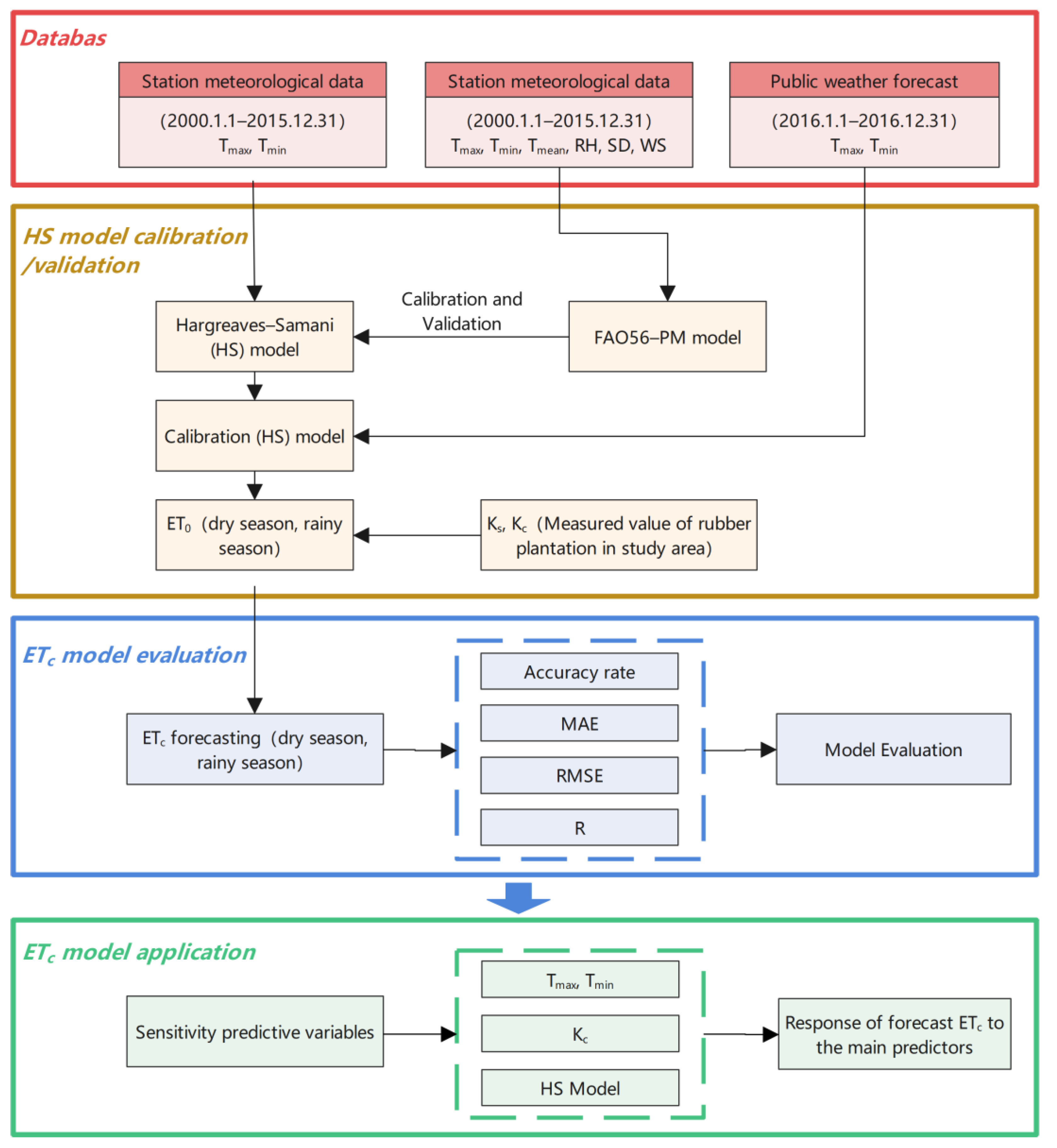
2. Materials and Methods

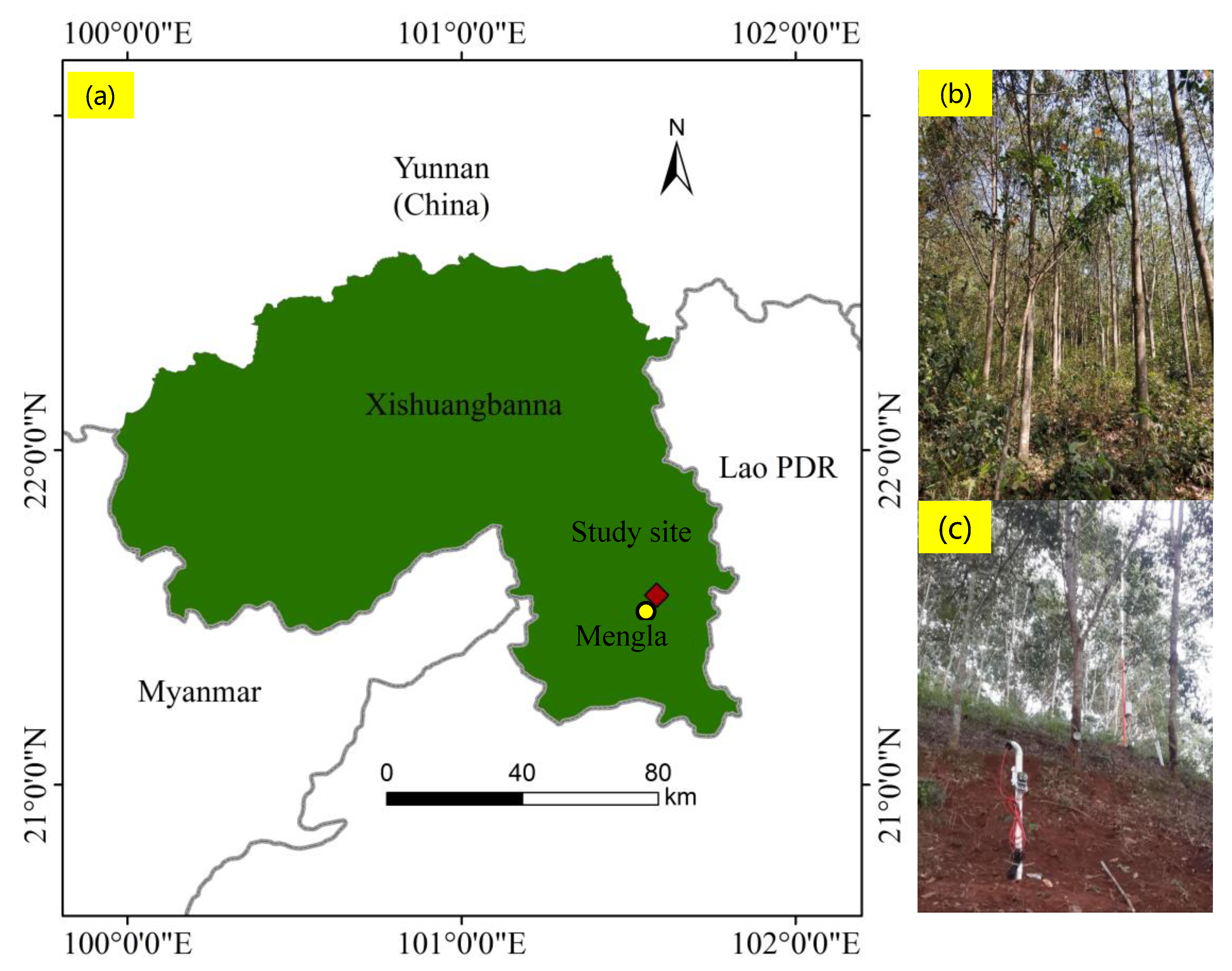
2.1. Study Area

The study site is located in Bubeng Village, Xishuangbanna, Southwest China (21°34′10″ N, 101°35′24″ E) (Figure 1). One of the meteorological observation stations sits up in Mengla (21°28′ N, 101°35′ E) near the Yunnan Meteorological Service Bureau. The average annual temperature is 21.5 °C. The average annual sunshine duration is 1853.4 h. The multi-year average annual rainfall was 1599 mm from 1970 to 2017, while the dry season (from November to April) only receives about 15% of the annual precipitation [5]. The rubber plantation of our study site was transformed from an original tropical monsoon forest with a slope length of approximately 300 m. Rubber trees were planted at 300 ± 50 trees ha⁻¹. A small number of shrubs and weeds grow under the rubber forest. The characteristics of the rubber plantation in the experimental site are presented in

Table 1. Characteristics of the rubber plantation and the experimental site.

Planting Year	Location	Altitude (m)	Slope (°)	Plot Area (m × m)	Mean Stem Diameter (cm)	Tree Height (m)	Planting Density (Trees/ha)
2001	21°34′10″ N 101°35′24″ E	726	22	200 × 200	17 ± 2	11.58 ± 2.3	300 ± 50

.

2.2. Data

2.2.1. Meteorological Data

The daily meteorological data for the period of 2000–2015 were collected from the China Meteorological Data Sharing Service System (http://cdc.cma.gov.cn, accessed on 23 November 2020) and Yunnan Meteorological Service Bureau. The trend of meteorological variables in Mengla is shown in Figure 2. The public weather forecast data from 2016 were acquired from Weather China (http://www.weather.com.cn, accessed on 12 December 2020). The framework of the rubber plantation ET_c forecast is shown in Figure 3. The weather forecast data include daily maximum air temperature (T_max) and daily minimum air temperature (T_min) forecasts for 7-day forecasting horizons, and the observed daily meteorological data include T_max and T_min, mean temperature (T_mean), relative humidity, average wind speed, and sunshine duration. ET₀ forecasts were calculated by the calibrated HS model using the temperature forecast data from 2016 as input parameters. The observed meteorological data were divided into three parts: the calibration period (2000–2012), the validation period (2013–2015), and 2016 was the test period.

Furthermore, the accuracy of ET₀ predictions was assessed by comparing the forecasted and calculated ET₀ values using observed weather data into the FAO56-PM model. Daily ET_c forecasts were based on ET₀ predictions using the temperature forecast and multiplied by values of the rubber crop coefficient (K_c) and the soil water stress coefficient (K_s). Finally, the proposed ET_c forecast method in our research was verified by comparing the ET_c forecast values with the observed values of the experimental sample site in 2016.

2.2.2. The Observed ET_c and Soil Water Content

The ET_c of the rubber plantation based on the meteorological and energy data measured by the Bowen ratio system at Mengla in the experimental sample site in 2016 are considered as observed ET_c to validate the model forecasting results. The volumetric water content (VWC, %) of soil moisture was automatically recorded at 10, 20, 30, and 40 cm depths, respectively, via sensors (ECH2O 5TE, Pullman, WA, USA) sampled. The ET_c was 1035.91 mm and the average daily ET_c was 2.83 mm d⁻¹. The ET_c was 630.19 mm in the rainy season, 211.67 mm in the cool-dry season, and 194.05 mm in the hot-dry season. The VWC values varied from 0.22 to 0.37 cm³/cm³ throughout the whole year.

2.3. Calculation of Reference Evapotranspiration

2.3.1. Hargreaves-Samani (HS) Model

The temperature and extraterrestrial-radiation-based Hargreaves-Samani (HS) model, as expressed in Equation (1), is used in the study to forecast daily ET₀ [29,45,46,47].

$$E{T}_{0,HS}=C\cdot R_a{(T_{\max }-T_{\min })}^E\cdot \left[(T_{\max }-T_{\min })/2+17.8\right]$$

(1)

where $E{T}_{0,HS}$ is the ET₀ value calculated by the HS model, mm d⁻¹; $R_a$ is the extraterrestrial radiation, MJ m⁻² d⁻¹; $T_{\max }$ and $T_{\min }$ are the maximum and minimum temperatures, °C; C is an empirical coefficient, which is 0.0023, and E is an exponent, which is 0.5 [46,48,49,50]. Values of parameters E and C need to be locally determined by calibration. The HS method has been recommended by the FAO as the alternative method to the PM method when meteorological data are limited [18].

2.3.2. Penman-Monteith Model

The Penman-Monteith method is recommended by the Food and Agriculture Organization of the United Nations (FAO) and the World Meteorological Organization (WMO) as the standard method by which to calculate ET₀ and for the evaluation of other methods [51,52,53,54]. Therefore, in this study, the ET₀ value calculated by the PM model was used as a standard reference to calibrate the parameters C and E of the HS model.

The PM method is expressed as follows:

$$E{T}_0=\frac{0.408\Delta (R_n-G)+\gamma \frac{900}{T+273}{u}_2(e_s-e_a)}{\Delta +\gamma (1+0.34u_2)}$$

(2)

where ET₀ is the reference crop evapotranspiration, mm d⁻¹; G is the soil heat flux, MJ m⁻² d⁻¹; R_n is the net canopy surface radiation, MJ m⁻² d⁻¹; u₂ is the mean wind speed at 2 m (which is converted from the wind speed at 10 m), m s⁻¹; T is the mean air temperature, °C; e_a is the actual water vapor pressure, kPa; e_s is the saturated water vapor pressure, kPa; γ is the hygrometer constant, kPa/°C; and Δ is the saturated water vapor pressure—temperature slope, kPa/°C.

The PM equation is established on physical and aerodynamic parameters, and thus produces reliable ET₀ results in most climates without local calibration. Many studies have also confirmed the superior performance of the PM method in various climates [51,52,53,54]. Thus, the PM method was used as a reference to calibrate the HS model based on the nonlinear least squares method in this study. The observed meteorological data were provided as an input into the PM equation and the output ET₀ results were used to quantify the accuracy of the forecasted ET₀ computed using the HS models.

2.3.3. Soil Water Stress Coefficient (K_s) and Crop Coefficient (K_c)

In the study, the ET_c of vegetation is calculated as follows:

$${\mathit{ET}}_c=K_s\times K_c\times {\mathit{ET}}_0$$

(3)

where ET_c is the crop evapotranspiration under nonstandard conditions, mm d⁻¹, and K_s is the soil water stress coefficient, and in rubber plantations it can be calculated using the following equation [55]:

$$K_s=\left\{\begin{array}{l}\hspace{1em}\hspace{1em}1,\hspace{1em}\begin{array}{lll}& & \theta \ge \end{array}{\theta }_{thr}\\ {\displaystyle \frac{\theta -{\theta }_{wp}}{{\theta }_{thr}-{\theta }_{wp}}},\begin{array}{ll}& {\theta }_{wp}\le \theta <{\theta }_{thr}\end{array}\end{array}\right.$$

(4)

where $\theta$ is the soil volume water content, %; ${\theta }_{{}_{wp}}$ is the soil volume water content at withering, %; and ${\theta }_{thr}$ is the critical the soil volume water content, %; where ${\theta }_{thr}=(1-p){\theta }_{fc}+p{\theta }_{wp}$, ${\theta }_{fc}$ is the field water holding capacity, %; $p$ is the ratio of water available in the rhizosphere to the total water, and, for the rubber plantation, is taken as 0.4 [18].

In our research, the observed ET_c value (as ET_c,obs) was measured by the Bowen ratio system at rubber plantations at the study site. The meteorological parameters monitored by automatic weather stations for the same time period were used for the calculation of the ET₀. The crop coefficient (K_c) in rubber plantations under nonstandard conditions was calculated as follows [56]:

$$K_c=\frac{E{T}_{c,obs}}{E{T}_0\cdot K_s}$$

(5)

All notations are as defined above.

2.4. Model Evaluation Criteria

To evaluate the accuracy of ET₀ forecasts using the HS model and ET_c forecasts of the rubber plantation in our study site, three indices, i.e., mean absolute error, MAE, root-mean-square error, RMSE, and correlation coefficient, R, were calculated as follows:

$$\mathit{MAE}={\displaystyle \sum _{i=1}^n\left|x_i-y_i\right|}/n$$

(6)

$$\mathit{RMSE}=\sqrt{{\displaystyle \sum _{i=1}^n{(x_i-y_i)}^2/n}}$$

(7)

$$R=\left[{\displaystyle \sum _{i=1}^n(x_i-x)(y_i-y)}\right]/\left[\sqrt{{\displaystyle \sum _{i=1}^n{(x_i-\overline{x})}^2}}\sqrt{{\displaystyle \sum _{i=1}^n{(y_i-\overline{y})}^2}}\right]$$

(8)

where $x_i$ is the forecasted value of each meteorological factor or the ET₀ value; $y_i$ is the observed value of each meteorological factor or the ET₀ value calculated by FAO56-PM; $i$ is the forecasted sample number ($i$ = 1, 2…); $\overline{x}$ is the average value of $x_i$; $\overline{y}$ is the average value of $y_i$; and $n$ is the number of forecast values. The statistical indices MAE, RMSE, and R for evaluating the accuracy of (i) forecast versus observed T_max and T_min, and ET₀, (ii) HS versus PM (ET₀ in calibration and validation), (iii) ET_c estimated versus ET_c were observed.

2.5. Sensitivity Analysis

To investigate the impact of the errors in input variables, T_max and T_min, and model parameter K_c on ET_c, a sensitivity analysis was performed using the mean values of the ET_c in the dry and rainy seasons as base values. ET_c was analyzed in terms of changes in T_max and T_min, and K_c values within a range of ±20% in 5% steps. During the process, ET_c values were computed using the proposed method by changing one parameter at a time while keeping the other parameters constant [57].

3. Results

3.1. Evaluation of Weather Forecast (T_max, T_min)

We compared the observed and forecasted temperature values at Mengla in Xishuangbanna (

Table 2. The T_max and T_min forecasts statistical index.

Lead Time (Day)	Tmax			Tmin
	MAE (°C)	RMSE (°C)	R	MAE (°C)	RMSE (°C)	R
1	1.74	2.37	0.84	1.39	1.87	0.93
2	1.76	2.43	0.85	1.42	1.88	0.93
3	1.76	2.45	0.84	1.49	1.96	0.91
4	1.77	2.49	0.83	1.84	2.52	0.85
5	1.93	2.71	0.81	1.77	2.33	0.87
6	2.01	2.89	0.77	1.92	2.41	0.83
7	2.10	3.16	0.75	1.91	2.44	0.83
Average	1.86	2.64	0.81	1.68	2.20	0.88

MAE, the average absolute error; R, the average correlation coefficient; RMSE, the root mean square error.

). It was seen that the accuracy of temperature forecasting declined with increasing lead time. The MAE, RMSE, and R of the T_max forecast ranged from 1.74 to 2.10 °C, 2.37 to 3.16 °C, and 0.84 to 0.75, respectively, for the lead time from 1 to 7 days. For the T_min forecast, the MAE, RMSE, and R ranged from 1.39 °C to 1.91 °C, 1.87 °C to 2.44 °C, and 0.93 to 0.83. The observed and forecasted temperature variables had strong linear relationships, as measured by the R values. All statistical indicators showed that the air temperature forecasts had good accuracy for ET_c forecasting.

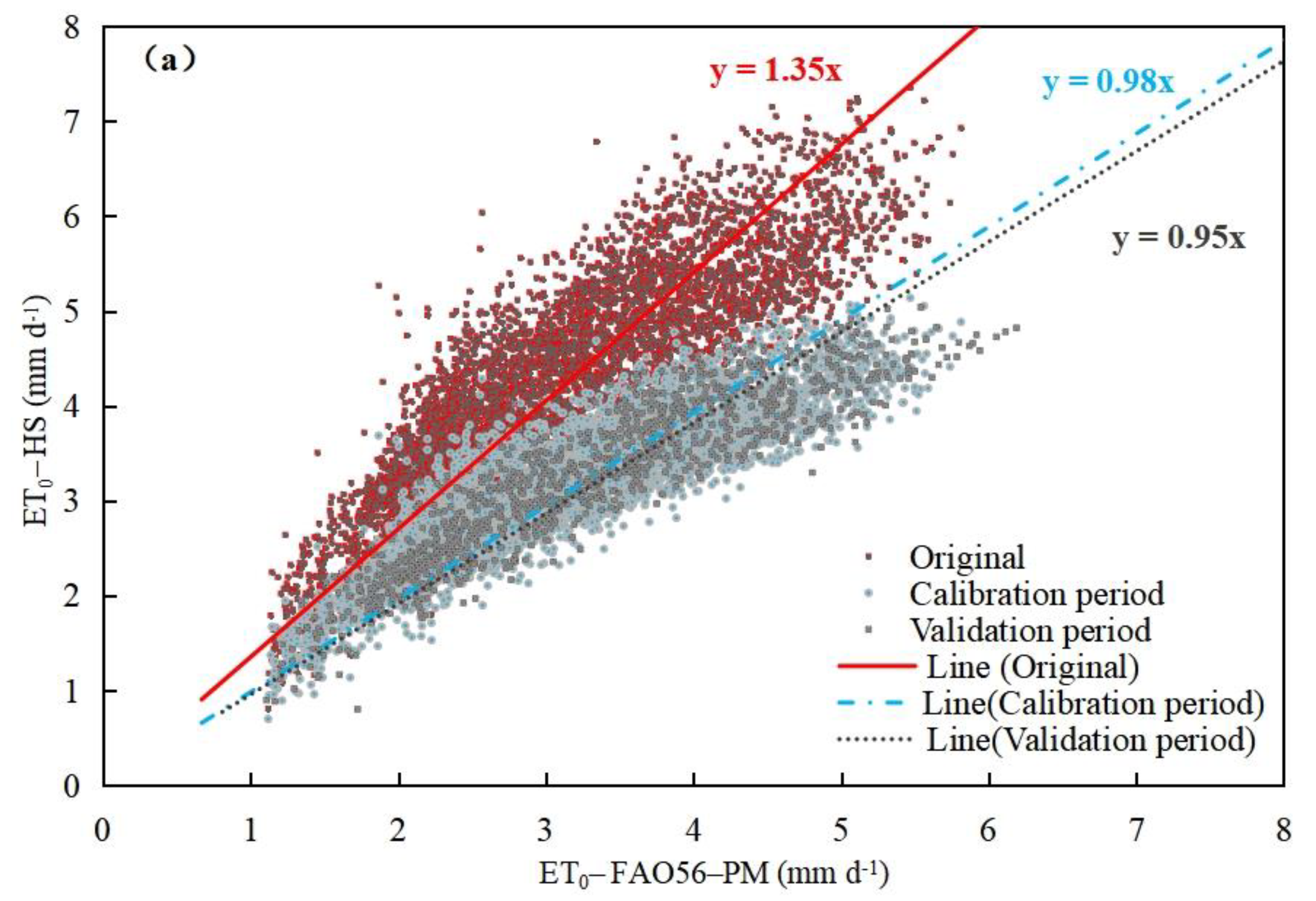
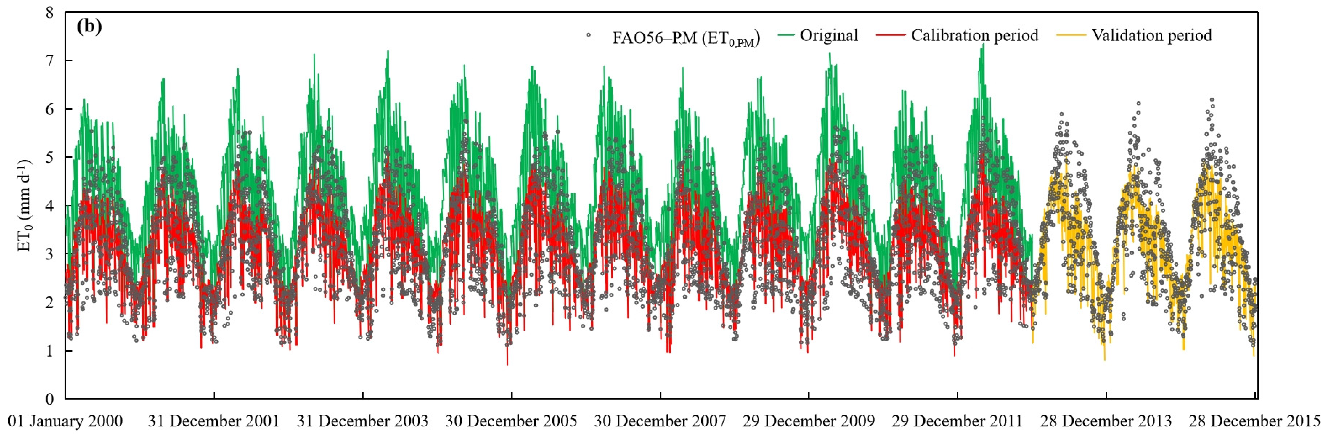
3.2. Calibration and Validation of the HS Model

The HS model was calibrated against the PM model using observed data; the optimized values for C and E were 0.002 and 0.43, respectively, which were different from the default parameter values (C was 0.0023 and E was 0.5) [46] due to the different area and climate conditions. However, the C and E values were close to the suggested values by Hu et al. [48], who calibrated the HS model against PM model over 105 climate stations in China.

The results showed that the calibrated HS model had great applicability in the study region. As shown in Figure 4a, the scatter plot of original data points calculated using default C and E values is biased with a slope of 1.35, and the ET₀ values calculated by the Hargreaves-Samani equation (as ET_0,HS) are much greater than the ET₀ values calculated by the Penman-Monteith equation (as ET_0,PM) (Figure 4b). After calibration, the slope of the linear correlation is 0.98, which is very close to 1, and in the validation period it is 0.95, indicating a very good performance (Figure 4a). In the calibration periods, the accuracy of MAE improved from 1.20 to 0.36; the RMSE improved from 1.30 to 0.45. In the validation periods, the accuracy of MAE improved from 1.20 to 0.35, the RMSE improved from 1.30 to 0.46 (

Table 3. Statistical indices of ET₀ calculated by the HS model.

	Original (2000–2015)			Calibration Period (2000–2012)			Validation Period (2013–2015)
	MAE (mm)	RMSE (mm d−1)	R	MAE (mm)	RMSE (mm d−1)	R	MAE (mm)	RMSE (mm d−1)	R
HS	1.20	1.30	0.88	0.36	0.45	0.89	0.35	0.46	0.91

). Figure 4b shows a time series comparison of ET_0,HS and ET_0,PM in the calibration and validation periods. Overall, the accuracy of the calibrated HS model could be used for forecasting ET₀ values in the study site.

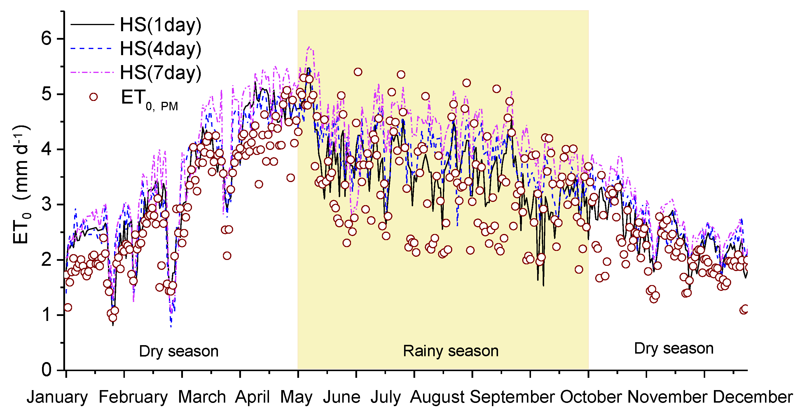
3.3. The Analysis of ET₀ Forecasts

The daily ET₀ forecast values (as ET_0,for) for 1-, 4-, and 7-day horizon forecasts and ET_0,PM for rubber plantations are displayed in Figure 5. The ET_0,for forecasts for rubber plantations range from 0.76 to 5.86 mm d⁻¹. Despite some over-predicted and under-predicted values, 1-, 4-, and 7-day horizon ET_0,for values follow the trend of ET_0,PM values.

The average values of the three statistical indicators of ET₀ for the dry and rainy seasons in the 1–7-d ahead forecasting period in Xishuangbanna are shown in

Table 4. Statistical indices of the ET₀ forecasts during 2016.

Lead Time (Day)	Dry Season			Rainy Season
	MAE (mm d−1)	RMSE (mm d−1)	R	MAE (mm d−1)	RMSE (mm d−1)	R
1	0.52	0.62	0.91	0.47	0.58	0.83
2	0.43	0.54	0.90	0.49	0.60	0.77
3	0.45	0.56	0.89	0.50	0.62	0.76
4	0.48	0.60	0.88	0.51	0.63	0.75
5	0.48	0.61	0.87	0.51	0.63	0.74
6	0.52	0.65	0.85	0.57	0.72	0.72
7	0.52	0.65	0.85	0.57	0.72	0.69
Average	0.49	0.60	0.88	0.52	0.64	0.75

. In the dry season, the MAE was 0.43 to 0.52 mm, RMSE was 0.54 to 0.65 mm, and R was 0.91 to 0.85. While, in the rainy season, the MAE was 0.47 to 0.57 mm, RMSE was 0.58 to 0.72 mm, and R was 0.83 to 0.69 (Table 4). The deviation of daily ET_0,for values during the rainy season was relatively lower than that during the dry season. The accuracy of the three statistical indicators indicated that the performance of the ET₀ forecast slightly decreased with the increase in lead time regardless of the dry season or the rainy season.

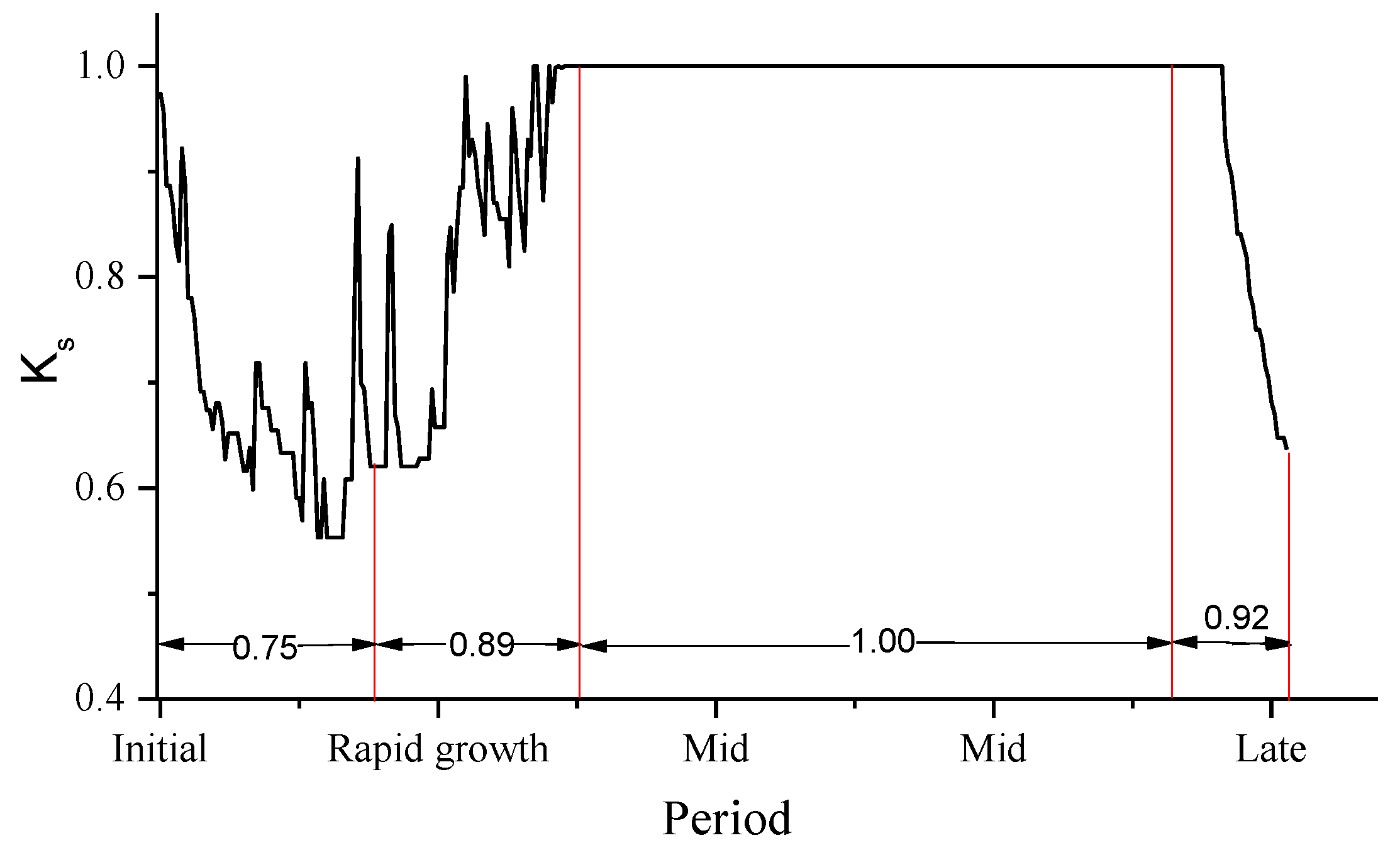
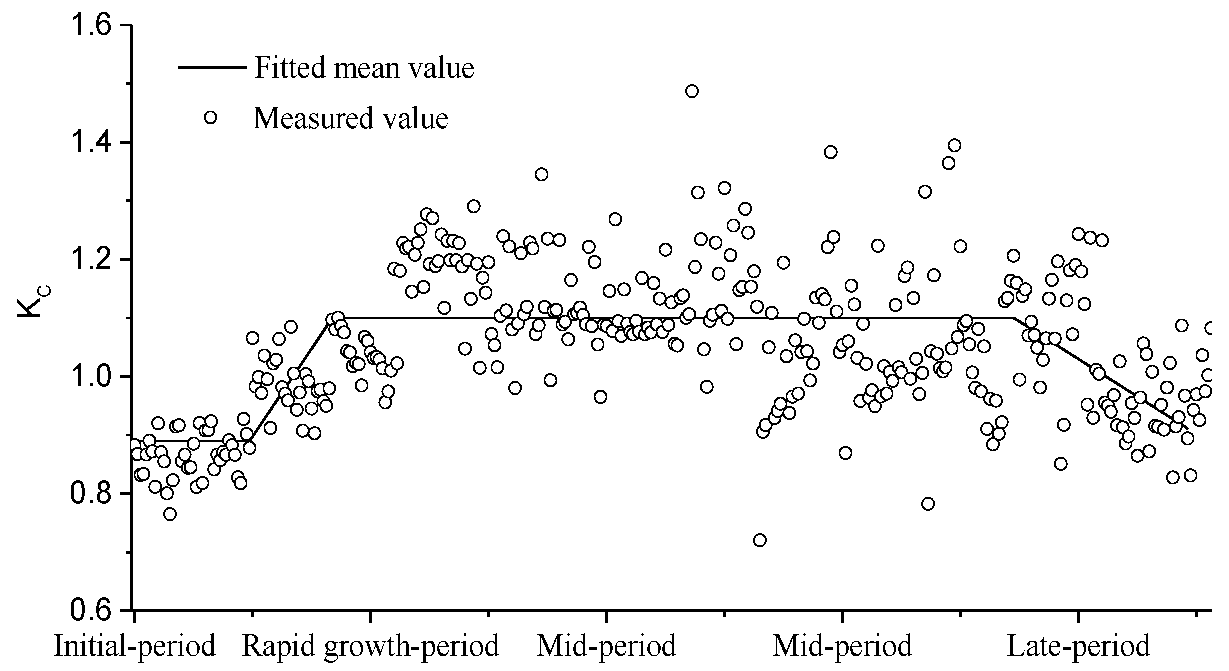
3.4. Results of Calculated Soil Water Stress Coefficient (K_s) and Crop Coefficient (K_c)

The growing season of the rubber plantation was split into four standard stages, i.e., the initial period, the rapid-growth period, the mid period, and the late period [18]. The length of the crop development stage at Xishuangbanna Tropical Botanical Garden follows that determined by the Chinese Academy of Science.

The Soil Water Stress Coefficient (K_s) was deduced with the measured soil water content of the rubber plantation sample site (Figure 6) that ranged from 0.55 to 1.00. The average values of K_s in each growing period of rubber plantations are as follows. In the initial-period, K_s is 0.75; in the rapid-growth period it is 0.89, in the mid period it is 1.00, and in the late period it is 0.92. While the crop coefficient (K_c) of rubber plantations calculated using Equation (5) (Figure 7) for the growing period ranges from 0.72 to 1.49. In the initial period, it is 0.89, in the mid period it is 1.10, and in the late period it is 0.91. The calculated K_c value in each growing period of the rubber plantations was taken as the basic parameter by which to calculate the multiyear ET_c of the rubber plantations in Xishuangbanna.

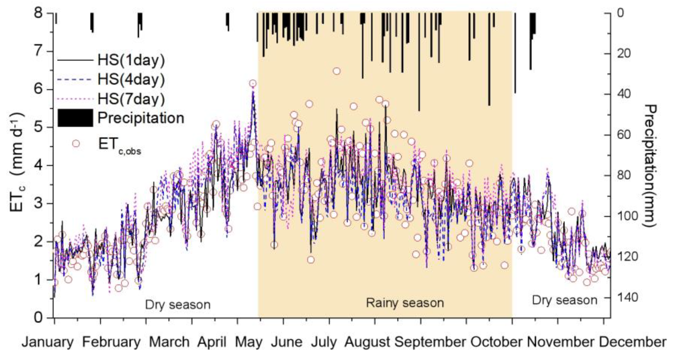
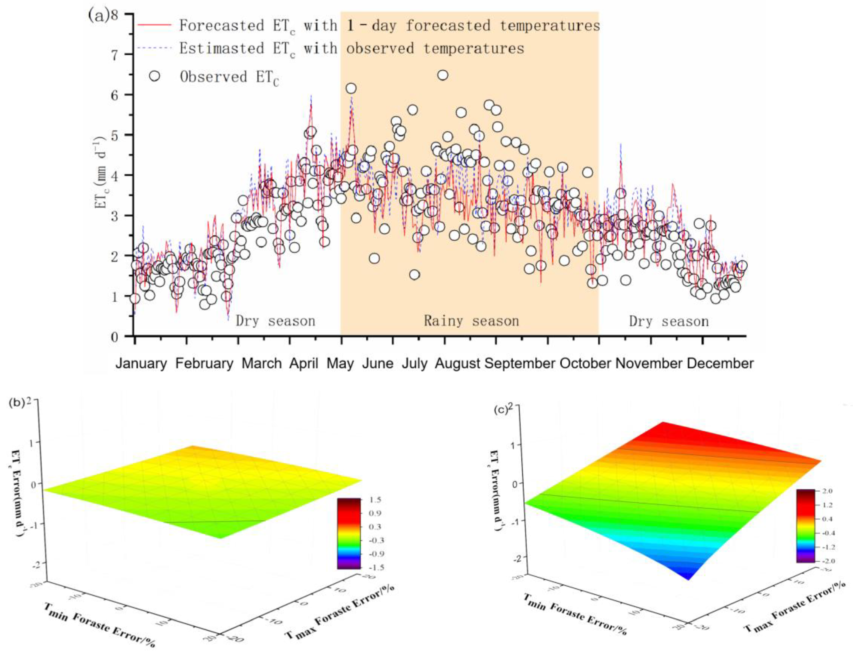
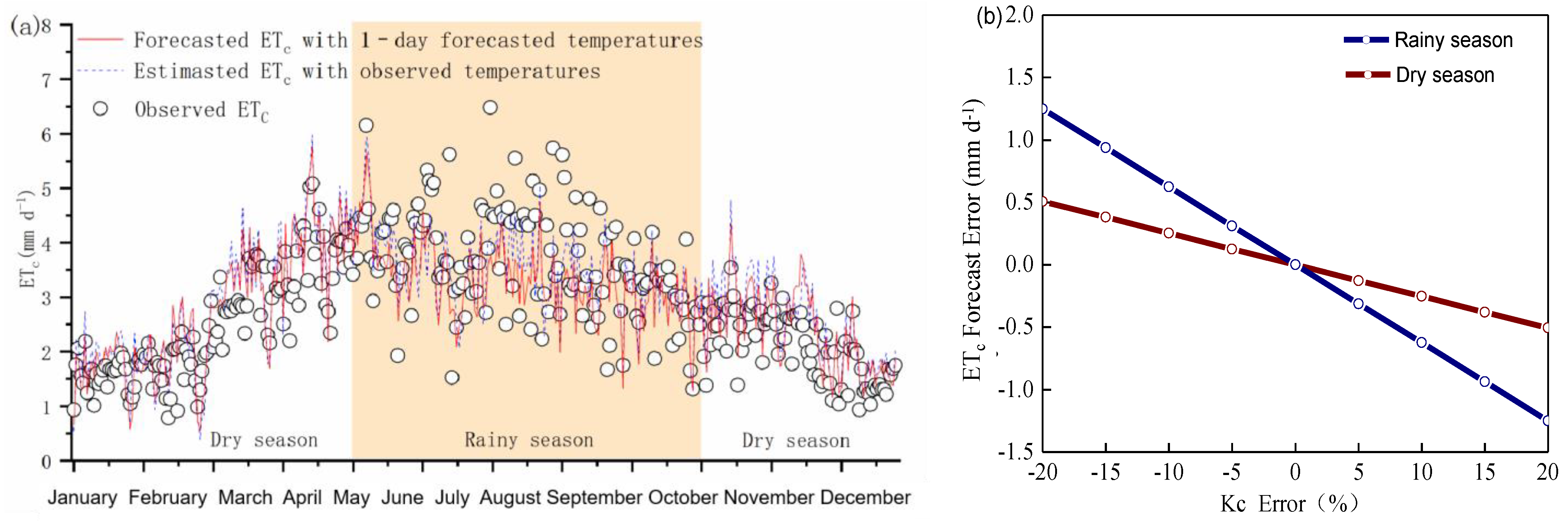
3.5. Performance of ET_c Forecasts

The forecast accuracy of the 7-day horizon forecast values compared with the ET_c values of the PM method in 2016 is presented in

Table 5. Forecast accuracy of ET_c in rubber plantations in 2016.

Lead Time (d)	Dry Season			Rainy Season
	MAE (mm d−1)	RMSE (mm d−1)	R	MAE (mm d−1)	RMSE (mm d−1)	R
1	0.64	0.85	0.82	0.57	0.73	0.70
2	0.61	0.82	0.80	0.59	0.75	0.69
3	0.62	0.83	0.80	0.60	0.77	0.68
4	0.62	0.84	0.81	0.63	0.81	0.65
5	0.61	0.82	0.81	0.64	0.82	0.65
6	0.63	0.84	0.80	0.65	0.83	0.65
7	0.65	0.85	0.79	0.65	0.83	0.65
Average	0.63	0.84	0.80	0.62	0.79	0.67

. The differences in the forecast values were not significant. In the rainy season, the MAE was 0.57–0.65 mm d⁻¹, RMSE was 0.73–0.83 mm d⁻¹, the R ranged from 0.70–0.65. While in the dry season, these values were 0.61–0.65 mm d⁻¹, 0.82–0.85 mm d⁻¹, and 0.82–0.79, respectively.

The variations of the 1-day, 4-day, and 7-day ET_c forecast values (as ET_c,for) and the precipitation during the dry season and the rainy season in 2016 are shown in Figure 8. The ET_c,for values followed the same variation patterns as the ET_c,obs values, and captured most of the important daily fluctuations for rubber plantations, except for a small number of predicted values. Precipitation in the rainy season (up to 1241.6 mm) is about four times that in the dry season (324 mm). The ET_c,for values have larger fluctuations than the measured ET_c,obs values in the rainy season.

3.6. The Results of the Sensitivity Analysis

The HS model has been commonly chosen in ET_c calculations due to its good performance and easy use. However, it is worth noting that the ET_c forecast has uncertainty associated with it.

The temperature forecast error directly affects the accuracy of ET₀ forecasts, which in turn leads to ET_c forecast errors. This study shows that ET_c forecasts are less influenced by temperature forecast errors; only −0.38 to 0.14 mm day⁻¹ in the rainy season for a 1-day forecast (Figure 9b). ET_c forecasts are more influenced by temperature forecast errors in the dry season when a ±20% temperature forest error results in a −1.47 to 0.94 mm day⁻¹ error in ET_c forecasts (Figure 9c).

Meanwhile, the ET_c errors also come from the mean values of K_c. For illustrative purposes, the effect of K_c error on ET_c forecast is shown in Figure 10, where it compares the ET_c,obs values and ET_c,for values for the 1-day lead time temperature forecast in 2016 (Figure 10a). In the dry season, the error between the forecasted ET_c with original K_c and with observed ET_c value is 11.39%. The error between the estimated ET_c with calibrated K_c and observed ET_c value is 3.91%. In the rainy season, the errors are −7.05% and −0.99%, respectively.

The sensitivity of the ET_c forecast to K_c is shown in Figure 10b. The ET_c forecast error is −0.51 to 0.51 mm day⁻¹ in the dry season and −1.24 to 1.24 mm d⁻¹ in the rainy season when the K_c error varies from −20% to 20%. The rainy season is the peak growing period of rubber trees with higher ET_c. The temperature forecast errors and the K_c value error vary from −20% to 20%; the ET_c forecast error is −0.38 to 0.14 mm d⁻¹ and −1.24 to 1.24 mm d⁻¹, respectively.

4. Discussion

In our research, a “K_c-ET₀” method was proposed to forecast the short-term daily ET_c of rubber plantations using weather forecast information and the HS model. ET₀ is the key to real-time ET_c forecasting. The quality of the weather forecasts is checked as it affects daily ET₀ forecasts. We analyzed the performance of temperature for a lead time of 1–7 days. For both T_max and T_min, the average R values ranged from 0.81 and 0.88, respectively; i.e., the observed and forecasted temperature variables had strong linear relationships. The T_min forecasts had a relatively better performance than that of T_max, and this result is in accordance with most of the previous findings in China [30,58,59]. We concluded that the accuracy of the minimum and maximum air temperature forecast was acceptable for ET_c forecasts in Xishuangbanna.

The HS model was calibrated using ET_0,PM. Due to the different area and climate conditions, the calibrated parameter C was 0.002, which agreed well with the original value (0.0023). The parameter E was 0.43 which was slightly lower than the original value of 0.50 [41]. The calibrated values of C and E for HS were suitable for the ET₀ modeling of Xishuangbanna. The calibrated ET₀ values calculated were closer to the line y = x compared with the PM method than the uncalibrated models, and with R = 0.91. Regional calibration increased the goodness-of-fit between all of the ET₀ values calculated by the HS model and ET_0,PM [60,61].

The changes in ET_0,for in the 1–7 day lead time strongly matched with ET_0,PM throughout the rubber plantation growing period. With the increase in lead time, the accuracy of the ET₀ forecast slightly decreased, which was caused by the decreasing accuracy of the temperature forecast mentioned above. The accuracy of ET₀ daily forecasts in the rainy season was slightly lower than in the dry season, which may be attributed to the HS model ignoring the effects of wind speed and relative humidity, which vary more in the rainy season [62]. However, the forecasted ET₀ results using the HS model were considered reliable for estimating ET_c, as revealed from the accuracy metrics.

The length of the crop development stage was different from that recommended by FAO-56, likely due to the differences in climate regions, elevation, crop varieties, and cropping conditions [18]. In our study, we considered the soil water stress coefficient (K_s), which is obtained through observed soil water content because rubber plantations are suffered from water stress during their growth period [63]. Then, the calculated K_c of different growth periods is closer to the actual local situation.

The initial K_c value (0.89) was slightly less than the value obtained by the procedure proposed by Allen et al. [18] (0.95). The K_c value for the mid period (1.10) was slightly larger than the value obtained by the process recommended by Allen et al. [18] (1.00). The late season K_c value (0.91) was lower than the value proposed by Allen et al. [18] (1.00). This deviation could be due to different rubber plantation varieties and climate regions, among others [4,13]. It should be noted that the K_c value was estimated based on 1-year experiment data in our research. Longer series of measured data is advisable to improve the accuracy of K_c estimation and the forecasting performance for ET_c [4].

The performance of ET_c,for in the dry season (R = 0.85) was better than that in the rainy season (R = 0.69). Precipitation can influence air temperature, which impacts the accuracy of the ET₀ forecasts, which, in turn, directly influences the accuracy of ET_c through “K_c-ET₀” method. No matter whether in the dry season or the rainy season, the accuracy of ET_c,for is slightly lower than that of ET_0,for, but fulfills the requirement of rubber plantations ET_c forecast. Compared with ET_c,obs, the deviation of ET_c,for values increased with the increase in forecast lead time. The forecast error is lower in the dry season than in the rainy season. Rubber plantations usually suffer from drought during the dry season, so accurate ET_c,for in the dry season could provide guidance pertaining to water allocation decisions.

The temperature forecast error, K_c, and the HS model are the main sources of uncertainty associated with ET_c forecasts. After sensitivity analysis, we found that the maximum positive error occurs when the maximum temperature forecast fluctuates by 20% and the minimum temperature forecast fluctuates by −20%, while the maximum negative error occurs when the maximum temperature forecast fluctuates by −20% and the minimum temperature forecast error fluctuates by 20%. The negative error is much larger than the positive error [24].

Both T_max and T_min forecasts may lead to errors, but, in general, its influence is relatively smaller than that caused by the K_c value error. Similar findings have been reported in the study of Zhang et al. [13], although with different vegetation types. The error is partly caused by the HS model. The HS model only considers temperature and extraterrestrial radiation, and does not consider wind speed and relative humidity. It leads to errors in ET₀ estimation, which in turn affect the accuracy of ET_c. This study shows that using the locally calibrated values of parameters C and E in the HS model largely improved the accuracy of ET₀ forecasting, especially in a tropical and subtropical monsoon region like Xishuangbanna [30,59]. Analysis of the overall results showed that the HS model was suitable for forecasting ET_c using the proposed approach.

The accuracy of rubber plantation ET_c forecasts is expected to be further improved when more meteorological variables are available and considered, or a more physical-based model is used to estimate ET₀.

5. Conclusions

Based on short-term weather forecasting and the HS model, the daily ET_c forecasting of a rubber plantation was conducted in the study. We evaluated the forecasting performance of ET_c by comparing observed data from actual rubber plantations at the experimental sites, analyzed the differences between the forecasting performances of rubber plantations, and also identified the ET_c forecasts error sources and their sensitivity. The following conclusions are drawn from the study.

(1)

The forecasting accuracy of ET_c based on the “K_c-ET₀” method in our research shows good performance and acceptable accuracy. The accuracy of ET_c forecasting in the dry season is higher than that in the rainy season. The results indicate that the proposed method is considered suitable for ET_c forecasting of rubber plantations in Xishuangbanna, Southwest China.

(2)

ET_c forecast errors come from temperature forecasts, the K_c value, and the HS model. The HS model does not consider meteorological variables such as wind speed and relative humidity. Using the locally optimized values of parameters, the results of HS method are significantly improved. Compared to the temperature forecast, the error in the K_c value has a larger impact on the error in the ET_c forecast. The accuracy of the K_c and forecasting performance for ET_c can be improved if the observation time of the actual data series is increased.

(3)

Our study provides reference information for forecasting ET_c using short-term weather forecast data and a theoretical basis for rubber plantations in Xishuangbanna. It is anticipated that the short-term forecasting approach of ET_c for rubber plantations as demonstrated in this study can be applied in larger regions for water management and the water use efficiency of rubber plantations, allowing irrigation managers and farmers to make ET-based irrigation schedules to increase the efficiency of water applications based on the plant water requirements and soil processes.

It is worth noting that the value of K_c, a key parameter of the ET_c forecast, in this study was taken from the results of limited field observations. With the increasing availability of Earth observation systems, the use of multispectral imagery such as LAI and albedo is expected to improve the accuracy of crop parameter estimation. Advances in weather forecasting and crop remote sensing will significantly contribute to the development of the optimal management of water resources in precision agriculture.

References

1. Liu, B.; Liu, M.; Cui, Y.; Shao, D.; Mao, Z.; Zhang, L.; Luo, Y. Assessing forecasting performance of daily reference evapotranspiration using public weather forecast and numerical weather prediction. J. Hydrol. 2020, 590, 125547. [Google Scholar] [CrossRef]
2. Qiu, R.; Liu, C.; Cui, N.; Wu, Y.; Wang, Z.; Li, G. Evapotranspiration estimation using a modified Priestley-Taylor model in a rice-wheat rotation system. Agric. Water Manag. 2019, 224, 105755. [Google Scholar] [CrossRef]
3. Kumagai, T.; Mudd, R.G.; Giambelluca, T.W.; Kobayashi, N.; Miyazawa, Y.; Lim, T.K.; Kasemsap, P. How do rubber (Hevea brasiliensis) plantations behave under seasonal water stress in northeastern Thailand and central Cambodia? Agric. For. Meteorol. 2015, 213, 10–22. [Google Scholar] [CrossRef] [Green Version]
4. Li, D.; Chen, J.; Luo, Y.; Liu, F.; Luo, H.; Xie, H.; Cui, Y. Short-term daily forecasting of crop evapotranspiration of rice using public weather forecasts. Paddy Water Environ. 2018, 16, 397–410. [Google Scholar] [CrossRef]
5. Ling, Z. Spatial-Temporal Variation Characteristics and Prediction Model of Evapotranspiration of Rubber Plantation in Xishuangbanna. Ph.D. Thesis, Yunnan Normal University, Kunming, China, 2021. [Google Scholar]
6. Tan, Z.; Zhang, Y.; Song, Q.; Liu, W.; Deng, X.; Tang, J.; Deng, Y.; Zhou, W.; Yang, L.; Yu, G.; et al. Rubber plantations act as water pumps in tropical China. Geophys. Res. Lett. 2011, 38, L24406. [Google Scholar] [CrossRef] [Green Version]
7. Giambelluca, T.W.; Mudd, R.G.; Liu, W.; Ziegler, A.D.; Kobayashi, N.; Kumagai, T.; Miyazawa, Y.; Lim, T.K.; Huang, M.; Fox, J.; et al. Evapotranspiration of rubber (Hevea brasiliensis) cultivated at two plantation sites in Southeast Asia. Water Resour. Res. 2016, 52, 660–679. [Google Scholar] [CrossRef] [Green Version]
8. Mohan, M.M.P.; Kanchirapuzha, R.; Varma, M.R.R. Review of approaches for the estimation of sensible heat flux in remote sensing-based evapotranspiration models. J. Appl. Remote Sens. 2020, 14, 041501. [Google Scholar] [CrossRef]
9. Kalua, M.; Rallings, A.M.; Booth, L.; Medellín-Azuara, J.; Carpin, S.; Viers, J.H. sUAS Remote Sensing of Vineyard Evapotranspiration Quantifies Spatiotemporal Uncertainty in Satellite-Borne ET Estimates. Remote Sens. 2020, 12, 3251. [Google Scholar] [CrossRef]
10. Niu, C.J.; Deng, W.; Gu, S.X.; Chen, G.; Liu, S.S. Real-time irrigation forecasting for ecological water in artificial wetlands in the Dianchi Basin. J. Inf. Optim. Sci. 2017, 38, 1181–1196. [Google Scholar] [CrossRef]
11. Pelosi, A.; Villani, P.; Bolognesi, S.; Chirico, G.; D’Urso, G. Predicting Crop Evapotranspiration by Integrating Ground and Remote Sensors with Air Temperature Forecasts. Sensors 2020, 20, 1740. [Google Scholar] [CrossRef] [Green Version]
12. Rochester, E.W.; Busch, C.D. An irrigation scheduling model which incorporates rainfall predictions. J. Am. Water Resour. Assoc. 1972, 8, 608–613. [Google Scholar] [CrossRef]
13. Zhang, L.; Cui, Y.; Xiang, Z.; Zheng, S.; Traore, S.; Luo, Y. Short-term forecasting of daily crop evapotranspiration using the ‘Kc-ET0’ approach and public weather forecasts. Arch. Agron. Soil Sci. 2018, 7, 903–915. [Google Scholar] [CrossRef]
14. Silva, D.; Meza, F.; Varas, E. Estimating reference evapotranspiration (ET0) using numerical weather forecast data in central Chile. J. Hydrol. 2010, 382, 64–71. [Google Scholar] [CrossRef]
15. Gu, S.; Zhao, Z.; Chen, J.; Chen, J.; Zhang, L. Daily potential evapotranspiration and meteorological drought prediction based on high-dimensional Copula function. Trans. CSAE 2020, 36, 151–159. [Google Scholar] [CrossRef]
16. Cunha, A.C.; Filho, L.R.A.G.; Tanaka, A.A.; Goes, B.C.; Putti, F.F. Influence of the estimated global solar radiation on the reference evapotranspiration obtained through the Penman-monteith FAO-56 method. Agric. Water Manag. 2021, 243, 106491. [Google Scholar] [CrossRef]
17. Elbeltagi, A.; Nagy, A.; Mohammed, S.; Pande, C.B.; Kumar, M.; Bhat, S.A.; Zsembeli, J.; Huzsvai, L.; Tamás, J.; Kovács, E.; et al. Combination of Limited Meteorological Data for Predicting Reference Crop Evapotranspiration Using Artificial Neural Network Method. Agronomy 2022, 12, 516. [Google Scholar] [CrossRef]
18. Allen, R.; Pereira, L.S.; Raes, D.; Smith, M. Crop Evapotranspiration-Guidelines for Computing Crop Water Requirements; FAO Irrigation & Drainage Paper No. 56; FAO: Rome, Italy, 1998. [Google Scholar]
19. Sarlak, N.; Bagcaci, S.C. The Assesment of Empirical Potential Evapotranspiration Methods: A Case Study of Konya Closed Basin. Teknik Dergi. 2020, 31, 9755–9772. [Google Scholar]
20. Aydin, Y. An Evaluation of the Hargreaves-Samani Method for Estimating Evapotranspiration Under Semi-Arid Conditions. Philipp. Agric. Sci. 2021, 104, 310–317. [Google Scholar]
21. Irmak, S.; Irmak, A.; Allen, R.; Jones, J. Solar and net radiation-based equations to estimate reference evapotranspiration in humid climate. ASCE J. Irrig. Drain. Eng. 2003, 129, 336–347. [Google Scholar] [CrossRef]
22. Smith, M. CLIMWAT for CROPWAT: A Climatic Database for Irrigation Planning and Management; FAO Irrigation and Drainage Paper No. 49; FAO: Rome, Italy, 1993; Available online: http://www.fao.org/land-water/databases-and-software/climwat-for-cropwat/en/ (accessed on 17 August 2019).
23. Kukal, M.; Irmak, S.; Walia, H.; Odhiambo, L. Spatio-temporal Calibration of Hargreaves-Samani Model to Estimate Reference Evapotranspiration across U.S. High Plains. Agron. J. 2020, 112, 4232–4248. [Google Scholar] [CrossRef]
24. Qian, K.; Chen, M.; Shen, Y.; Hu, X.; Jin, L.; Liu, S.; Cui, Y.; Luo, Y. Comparison and Sensitivity Analysis of Reference Crop Evapotranspiration Prediction Models in the Sanjiang Plain Based on Public Weather Forecasting. Water Sav. Irrig. 2021, 308, 62–67. (In Chinese) [Google Scholar] [CrossRef]
25. Ferreira, L.B.; Duarte, A.B.; Araujo, E.D.; Ferreira, T.D.; da Cunha, F.F. Reference evapotranspiration estimated from air temperature using the mars regression technique. Biosci. J. 2018, 34, 674–682. [Google Scholar] [CrossRef] [Green Version]
26. Santos, J.E.O.; Cunha, F.F.; da Filgueiras, R.; Silva, G.H.; da Castro Teixeira, A.H.; de Santos Silva, F.C.; dos Sediyama, G.C. Performance of SAFER evapotranspiration using missing meteorological data. Agric. Water Manag. 2020, 233, 106076. [Google Scholar] [CrossRef]
27. Ballesteros, R.; Ortega, J.F.; Moreno, M.Á. FORETo: New software for reference evapotranspiration forecasting. J. Arid. Environ. 2016, 124, 128–141. [Google Scholar] [CrossRef]
28. Qiu, R.; Luo, Y.; Wu, J.; Zhang, B.; Liu, Z.; Agathokleous, E.; Yang, X.; Hu, W.; Clothier, B. Short–term forecasting of daily evapotranspiration from rice using a modified Priestley–Taylor model and public weather forecasts. Agric. Water Manag. 2023, 277, 108123. [Google Scholar] [CrossRef]
29. Luo, Y.; Chang, X.; Peng, S.; Khan, S.; Wang, W.; Zheng, Q.; Cai, X. Short-term forecasting of daily reference evapotranspiration using the hargreaves-samani model and temperatureforecasts. Agric. Water Manag. 2014, 136, 42–51. [Google Scholar] [CrossRef]
30. Yang, Y.; Cui, Y.; Bai, K.; Luo, T.; Dai, J.; Wang, W.; Luo, Y. Short-term forecasting of daily reference evapotranspiration using the reduced-set PenmanMonteith model and public weather forecasts. Agric. Water Manag. 2019, 211, 70–80. [Google Scholar] [CrossRef]
31. Zhang, L.; Zhao, X.; Ge, J.; Zhang, J.; Traore, S.; Fipps, G.; Luo, Y. Evaluation of Five Equations for Short-Term Reference Evapotranspiration Forecasting Using Public Temperature Forecasts for North China Plain. Water 2022, 14, 2888. [Google Scholar] [CrossRef]
32. Vijayakumar, K.; Dey, S.; Chandrasekhar, T.; Devakumar, A.; Sethuraj, M. Irrigation requirement of rubber trees (Hevea brasiliensis) in the subhumid tropics. Agric. Water Manag. 1998, 35, 245–259. [Google Scholar] [CrossRef]
33. Ziegler, A.; Fox, J.; Xu, J. The rubber juggernaut. Science 2009, 324, 1024–1025. [Google Scholar] [CrossRef]
34. Huang, X.; Li, X.; Mu, X.; Yuan, H.; Liang, Q.; Yao, P.; Yu, F. Study on regional vegetation water suitability: Based on the review of seasonal drought in Southwest China. Bull. Soil Water Conserv. 2014, 34, 301–307. [Google Scholar]
35. Chiarelli, D.D.; Passera, C.; Rulli, M.C.; Rosa, L.; Ciraolo, G.; D’Odorico, P. Hydrological consequences of natural rubber plantations in Southeast Asia. Land Degrad. Dev. 2020, 31, 2060–2073. [Google Scholar] [CrossRef]
36. Lin, Y.X.; Zhang, Y.P.; Zhao, W.; Zhang, X.; Dong, Y.X.; Fei, X.H.; Li, J. Comparison of transpiration characteristics of rubber forests with different stand ages. Chin. J. Ecol. 2016, 35, 855–863. [Google Scholar] [CrossRef]
37. Kobayashi, N.; Kumagai, T.; Miyazawa, Y.; Matsumoto, K.; Tateishi, M.; Lim, T.K.; Mudd, R.G.; Ziegler, A.D.; Giambelluca, T.W.; Yin, S. Transpiration characteristics of a rubber plantation in central Cambodia. Tree Physiol. 2014, 34, 285–301. [Google Scholar] [CrossRef] [Green Version]
38. Gonkhamdee, S.; Maeght, J.-L.; Do, F.C.; Pierret, A. Growth dynamics of fine Hevea brasiliensis roots along a 4.5-m soil profile. Khon Kaen Agric. J. 2009, 37, 265–276. [Google Scholar]
39. Gu, S.; He, D.; Cui, Y.; Xie, X.; Li, Y. Spatial variability of irrigation factors and their relationships with “corridor-barrier” functions in the Longitudinal Range-Gorge Region. Chin. Sci. Bull. 2007, 52, 33–41. [Google Scholar] [CrossRef]
40. Mokhtar, A.; He, H.M.; Alsafadi, K.; Mohammed, S.; Ayantobo, O.O.; Elbeltagi, A.; Abdelwahab, O.M.M.; Zhao, H.F.; Quan, Y.; Abdo, G.H.; et al. Assessment of the effects of spatiotemporal characteristics of drought on crop yields in southwest China. Int. J. Climatol. 2021, 42, 3056–3075. [Google Scholar] [CrossRef]
41. Seneviratne, S.; Corti, T.; Davin, E.; Hirschi, M.; Jaeger, E.; Lehner, I.; Orlowsky, B.; Teuling, A. Investigating soil moisture-climate interactions in a changing climate: A review. Earth Sci. Rev. 2010, 99, 125–161. [Google Scholar] [CrossRef]
42. Zhou, W.; Wu, Z.; He, Q.; Lu, C.; Jie, M. Rubber planting and drinking water shortage: A case of Goniu village in Xishuangbanna. Chin. J. Ecol. 2011, 30, 1570–1574. [Google Scholar] [CrossRef]
43. Chiarelli, D.D.; Rosa, L.; Rulli, M.C.; D’Odorico, P. The water-land-food nexus of natural rubber production. J. Clean. Prod. 2018, 172, 1739–1747. [Google Scholar] [CrossRef] [Green Version]
44. Mangmeechai, A. Effects of Rubber Plantation Policy on Water Resources and Landuse Change in the Northeastern Region of Thailand. Geogr. Environ. Sustain. 2020, 13, 73–83. [Google Scholar] [CrossRef]
45. Hargreaves, G.H.; Samani, Z.A. Reference Crop Evapotranspiration from Temperature. Appl. Eng. Agric. 1985, 1, 96–99. [Google Scholar] [CrossRef]
46. Hargreaves, G.H.; Allen, R.G. History and Evaluation of Hargreaves Evapotranspiration Equation. J. Irrig. Drain. Eng. 1985, 129, 53–63. [Google Scholar] [CrossRef]
47. Paredes, P.; Pereira, L.S.; Almorox, J.; Darouich, H. Reference grass evapotranspiration with reduced data sets: Parameterization of the FAO Penman-Monteith temperature approach and the Hargeaves-Samani equation using local climatic variables. Agric. Water Manag. 2020, 240, 106210. [Google Scholar] [CrossRef]
48. Hu, Q.; Yang, D.; Wang, Y.; Yang, H. Global Calibration and Applicability Evaluation of Hargreaves Equation. Adv. Water Sci. 2011, 22, 160–167. [Google Scholar] [CrossRef]
49. Martí, P.; Zarzo, M.; Vanderlinden, K.; Girona, J. Parametric expressions for the adjusted Hargreaves coefficient in Eastern Spain. J. Hydrol. 2015, 529, 1713–1724. [Google Scholar] [CrossRef]
50. Morales-Salinas, L.; Ortega-Farías, S.; Riveros-Burgos, C.; Neira-Román, J.; Carrasco-Benavides, M.; López-Olivari, R. Monthly calibration of Hargreaves-Samani equation using remote sensing and topoclimatology in central-southern Chile. Int. J. Remote Sens. 2017, 38, 7497–7513. [Google Scholar] [CrossRef]
51. Jensen, M.E.; Burman, R.D.; Allen, R.G. Evapotranspiration and Irrigation Water Requirements; American Society of Civil Engineers: Reston, VA, USA, 2016. [Google Scholar] [CrossRef]
52. Allen, R.G.; Smith, M.; Perrier, A.; Pereira, L.S. An update for the defnition of reference evapotranspiration. J. Environ. Sci. Health 1994, 43, 1–35. [Google Scholar]
53. Singh, P.K.; Patel, S.K.; Jayswal, P.; Chinchorkar, S.S. Usefulness of class A Pan coefcient models for computation of reference evapotranspiration for a semi-arid region. Mausam 2014, 65, 521–528. [Google Scholar] [CrossRef]
54. Arellano, M.G.; Irmak, S. Reference (Potential) Evapotranspiration. I: Comparison of Temperature, Radiation, and Combination-Based Energy Balance Equations in Humid, Subhumid, Arid, Semiarid, and Mediterranean-Type Climates. J. Irrig. Drain. Eng. 2016, 142, 04015065. [Google Scholar] [CrossRef]
55. Luo, Y.; Khan, S.; Cui, Y.; Peng, S. Application of system dynamics approach for time varying water balance in aerobic paddy fields. Paddy Water Environ. 2009, 7, 1–9. [Google Scholar] [CrossRef]
56. Allen, R. Using the FAO-56 dual crop coefficient method over an irrigated region as part of an evapotranspiration intercomparison study. J. Hydrol. 2000, 229, 27–41. [Google Scholar] [CrossRef]
57. Singh, V.P.; Xu, C.-Y. Sensitivity of mass-transfer-based evaporation equations to errors in daily and monthly input data. Hydrol. Process. 1997, 11, 1465–1473. [Google Scholar] [CrossRef]
58. Xiong, Y.; Luo, Y.; Wang, Y.; Traore, S.; Xu, J.; Jiao, X.; Fipps, G. Forecasting daily reference evapotranspiration using the Blaney–Criddle model and temperature forecasts. Arch. Agron. Soil Sci. 2016, 62, 790–805. [Google Scholar] [CrossRef]
59. Zhang, L.; Traore, S.; Cui, Y.; Luo, Y.; Zhu, G.; Liu, B.; Fipps, G.; Karthikeyan, R.; Singh, V. Assessment of spatiotemporal variability of reference evapotranspiration and controlling climate factors over decades in China using geospatial techniques. Agric. Water Manag. 2019, 213, 499–511. [Google Scholar] [CrossRef]
60. Awal, R.; Habibi, H.; Fares, A.; Deb, S. Estimating Reference Crop Evapotranspiration under Limited Climate Data in West Texas. J. Hydrol. Reg. Stud. 2020, 28, 100677. [Google Scholar] [CrossRef]
61. Rodrigues, G.C.; Braga, R.P. Estimation of Reference Evapotranspiration during the Irrigation Season Using Nine TemperatureBased Methods in a Hot-Summer Mediterranean Climate. Agriculture 2021, 11, 124. [Google Scholar] [CrossRef]
62. Perera, K.; Western, A.; Nawarathna, B.; George, B. Forecasting daily reference evapotranspiration for Australia using numerical weather prediction outputs. Agric. For. Meteorol. 1997, 194, 50–63. [Google Scholar] [CrossRef]
63. Ling, Z.; Shi, Z.; Gu, S.; He, G.; Liu, X.; Wang, T.; Zhu, W.; Gao, L. Estimation of Applicability of Soil Model for Rubber (Hevea brasiliensis) Plantations in Xishuangbanna. Southwest China Water 2022, 14, 295. [Google Scholar] [CrossRef]
Figure 1. The experimental site of a rubber plantation (indicated by a solid square; 21°34′10″ N, 101°35′24″ E) in Xishuangbanna, Yunnan Province, Southwest China. Mengla indicated by a yellow circle (21°28′ N, 101°35′ E) (a) Location of area; (b) Observed sample rubber plantation; (c) Automatic meteorological system stations (WS-BR06, Campbell, CA, USA) and Drain gauge G3 (METER, Pullman, WA, USA).
Agronomy 13 01013 g001
Figure 2. Trend of meteorological variables at Mengla Meteorological Station from 2000 to 2015.
Agronomy 13 01013 g002
Figure 3. Framework of the rubber plantation ETc forecast integrating public weather forecast data with the “Kc-ET0” method using the HS model. (RH, relative humidity; SD, sunshine duration; WS,wind speed; ET0, reference evapotranspiration; ETc, crop evapotranspiration; Kc, the crop coefficient; Ks, soil water stress coefficient; MAE, the average absolute error; R, the average correlation coefficient; RMSE, the root mean square error).
Agronomy 13 01013 g003
Figure 4. (a,b) The ET0 calibration and validation of the HS model.
Agronomy 13 01013 g004aAgronomy 13 01013 g004b
Figure 5. The ET0 for 1-, 4-, and 7-day forecast periods and the daily variation of ET0,PM in 2016 (1 January 2016–31 December 2016).
Agronomy 13 01013 g005
Figure 6. The soil water stress coefficient (Ks) of rubber plantations.
Agronomy 13 01013 g006
Figure 7. The crop coefficient (Kc) of rubber plantations.
Agronomy 13 01013 g007
Figure 8. ETc,for for 1-, 4-, and 7-day forecasts and daily observed ETc values.
Agronomy 13 01013 g008
Figure 9. The influence of temperatures on ETc,for (a) 1-day forecast and observed temperatures; (b) multi-factor method on error sensitivity analysis based on Tmin and Tmax in the rainy season; (c) multi-factor method on error sensitivity analysis based on Tmin and Tmax in the dry season.
Agronomy 13 01013 g009
Figure 10. The influence of Kc on ETc,for (a) comparisons of original Kc values and calibrated Kc values; (b) single factor method on Kc error on ETc forecast sensitivity analysis.
Agronomy 13 01013 g010