
Identification of Soybean Planting Areas Combining Fused Gaofen-1 Image Data and U-Net Model

 , and
, and
Abstract
:1. Introduction
2. Materials and Methods
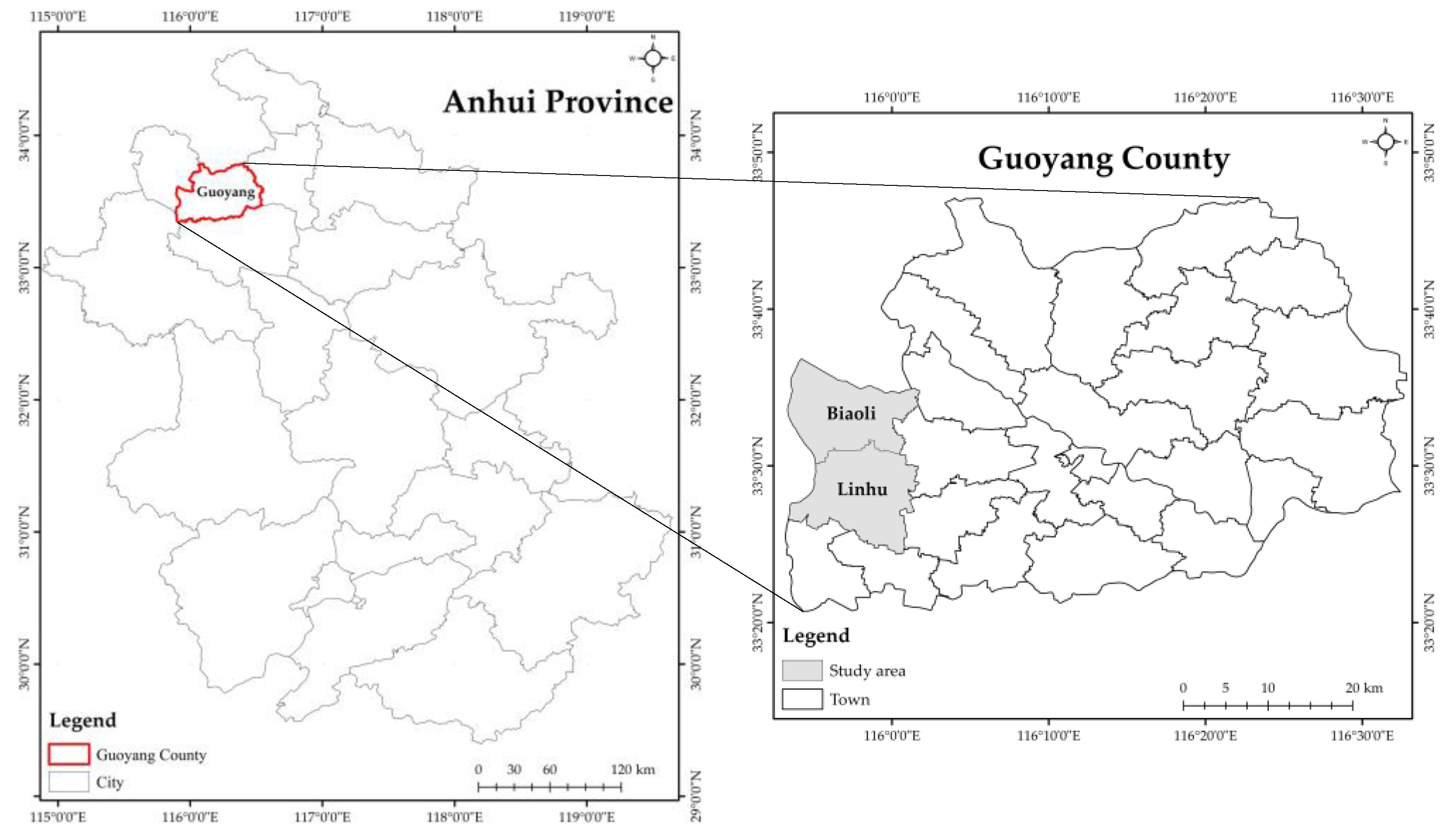
2.1. Study Area
2.2. Growth Stages of Soybean
2.3. Data Sources and Preprocessing
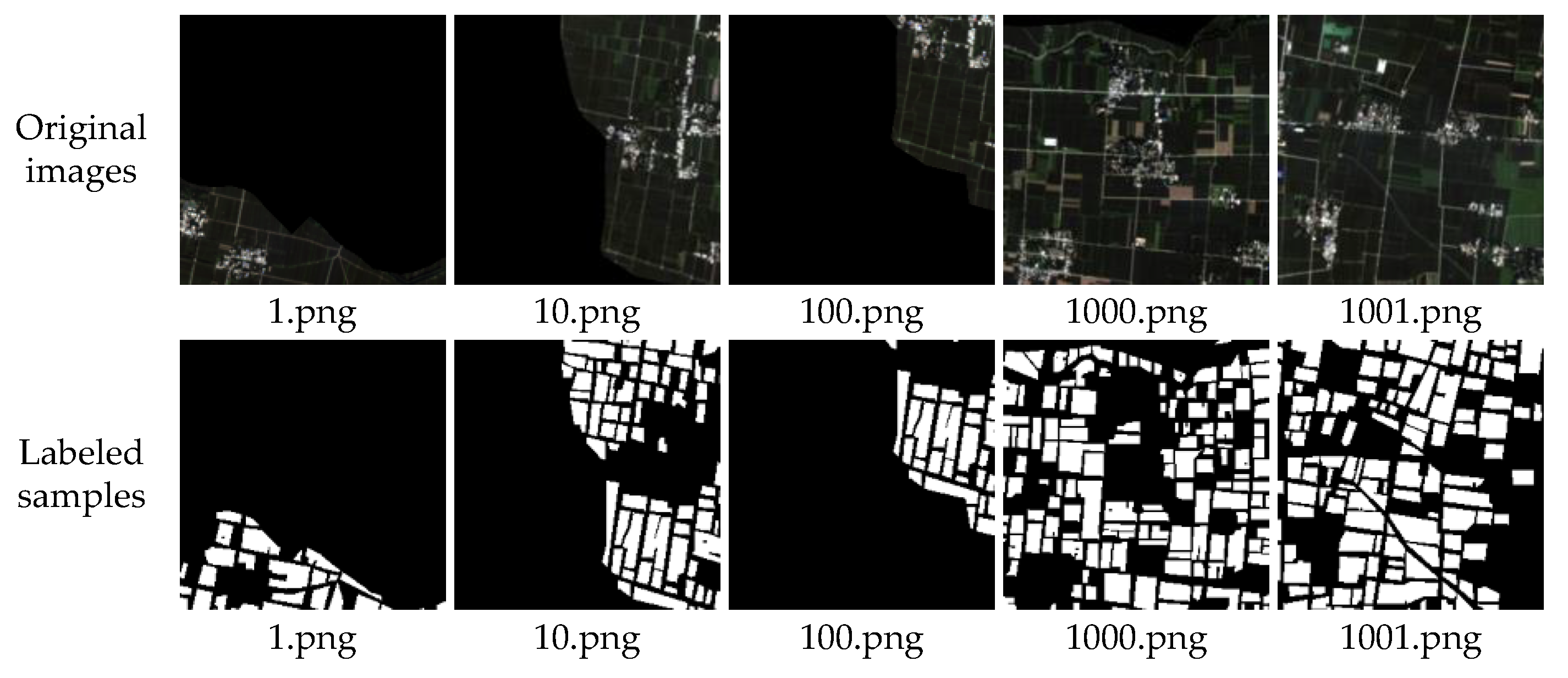
2.4. Dataset Production
- (1)
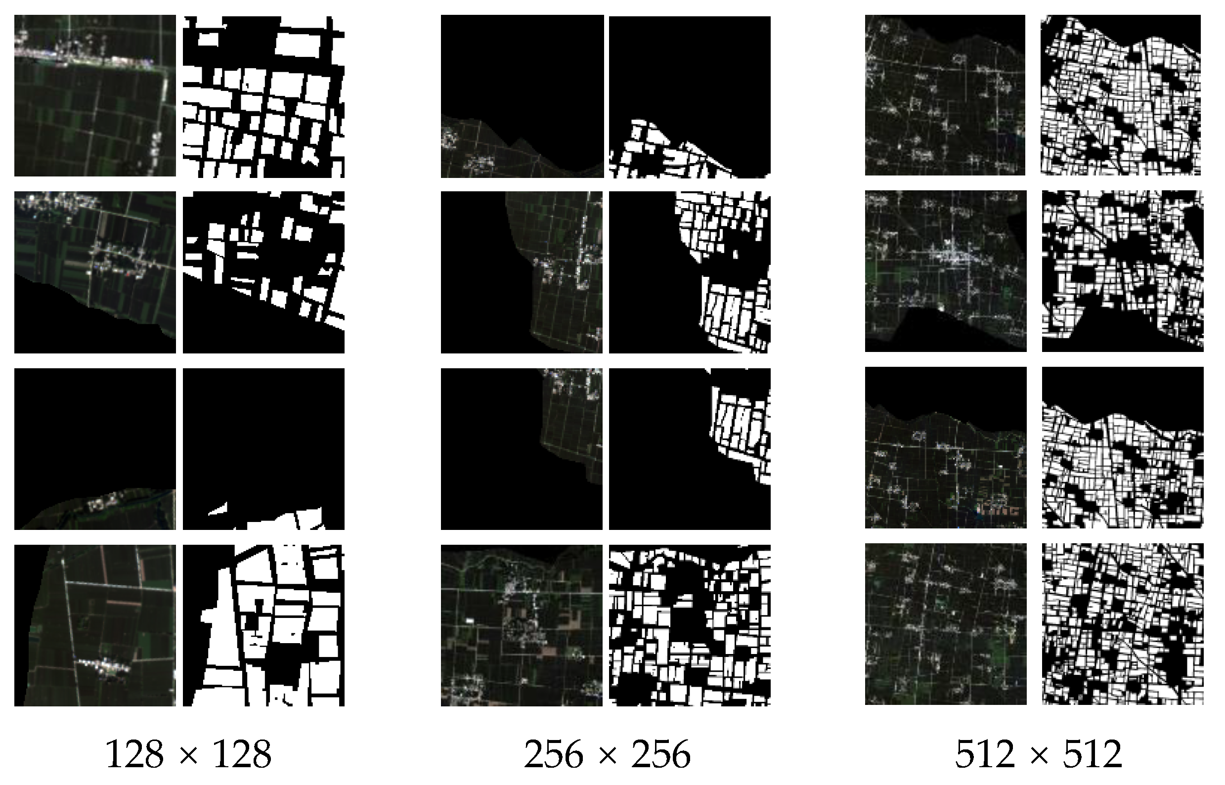
- Image cropping
- (2)
- Training and test datasets
- (3)
- Data normalization
- (4)
- Data augmentation
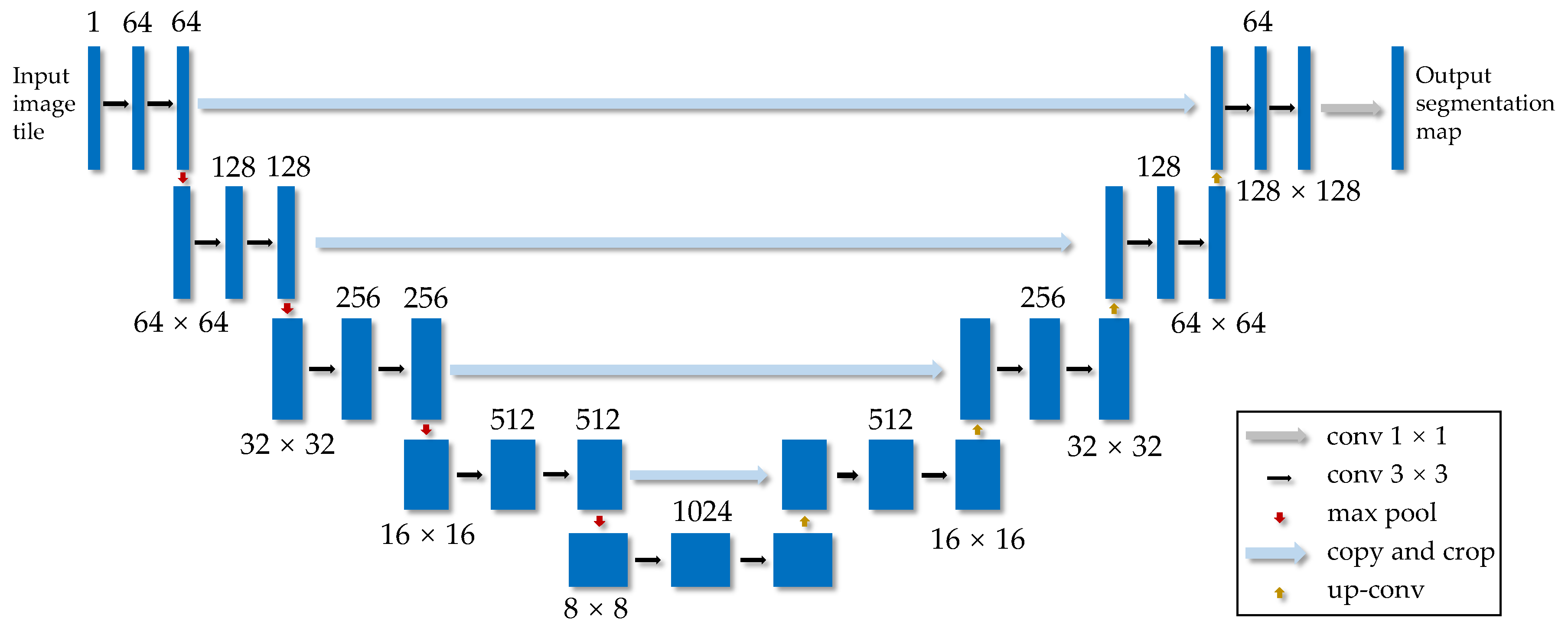
2.5. U-Net Model
2.6. Evaluation Metrics
3. Results and Discussion
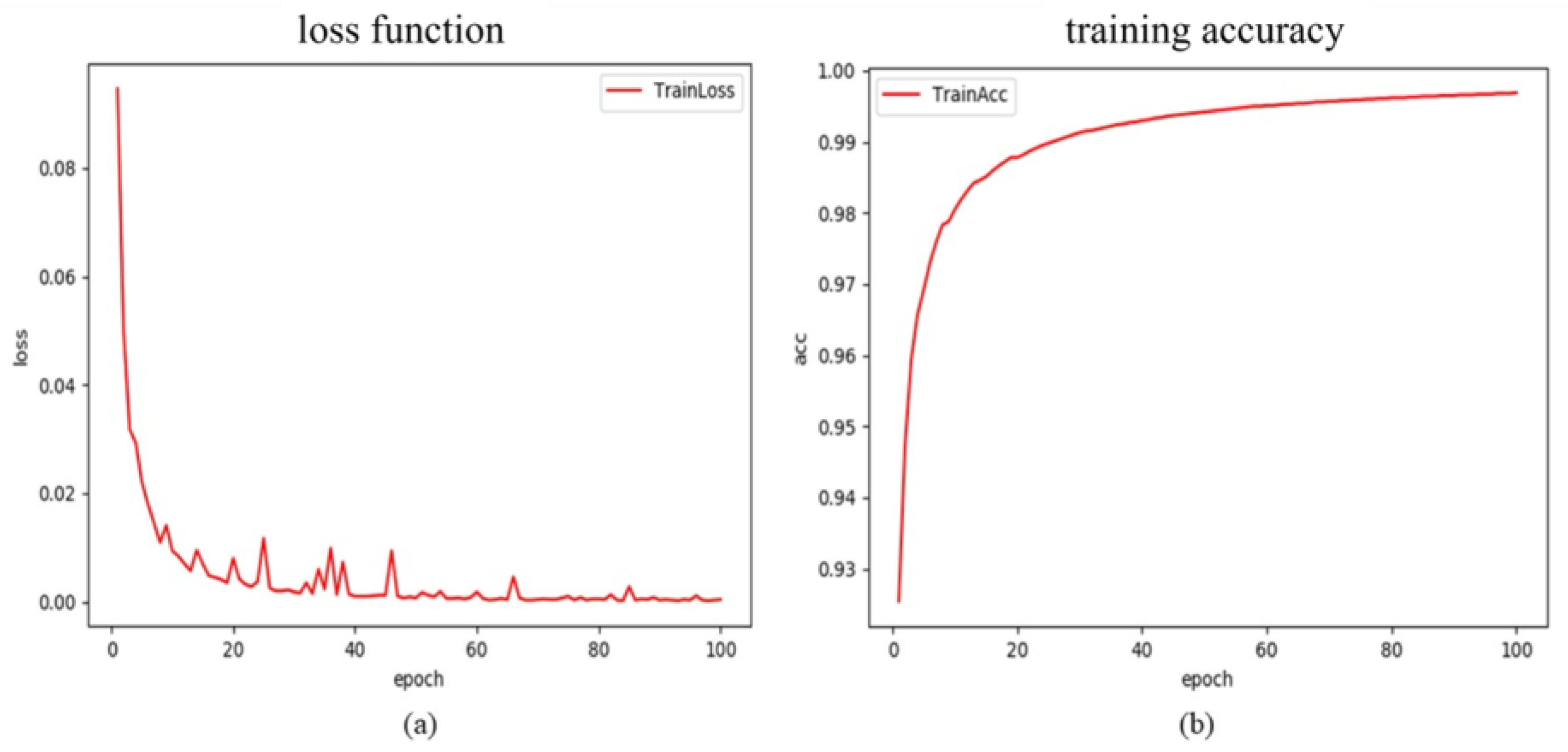
3.1. Model Training
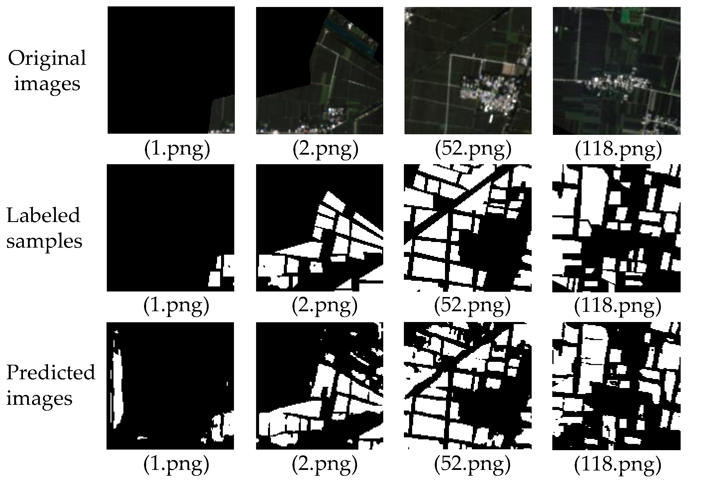
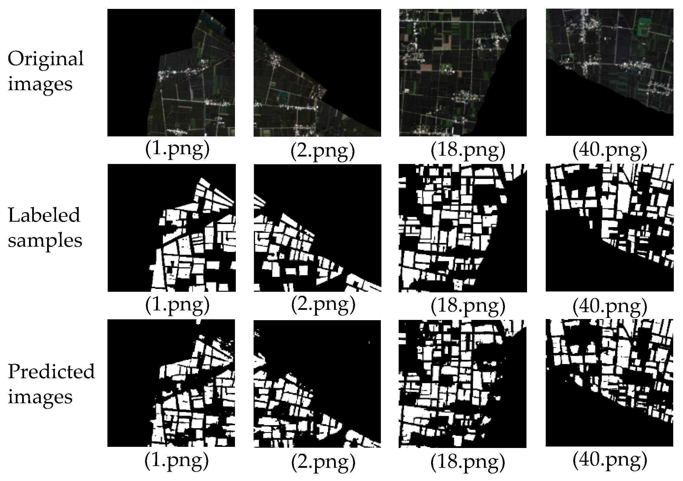
3.2. Influence of Cropping Size on Prediction Accuracy
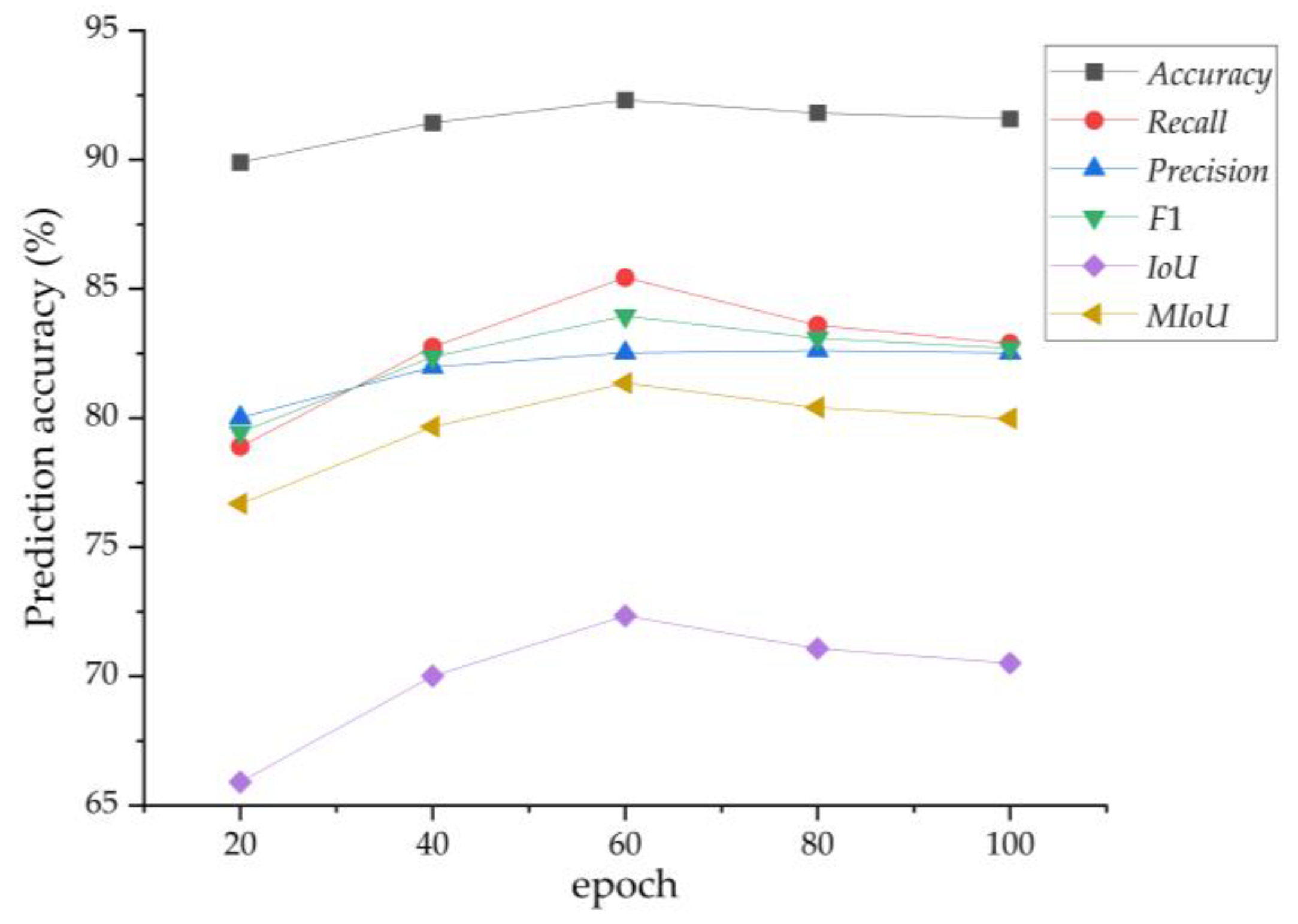
3.3. Influence of Training Epochs on Prediction Accuracies
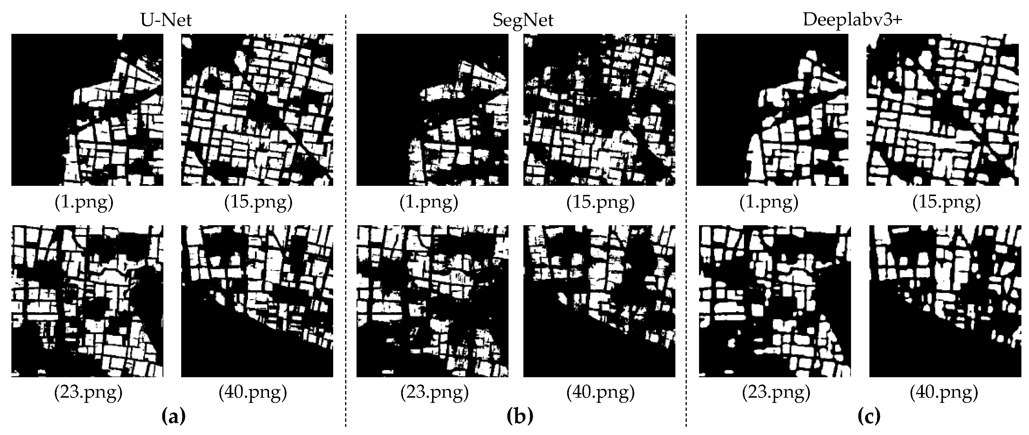
3.4. Comparison of Prediction Accuracies among Different Models
4. Conclusions
Author Contributions
Funding
Data Availability Statement
Conflicts of Interest
References
- Liu, X.; Jin, J.; Wang, G.; Herbert, S.J. Soybean yield physiology and development of high-yielding practices in Northeast China. Field Crop. Res. 2008, 105, 157–171. [Google Scholar] [CrossRef]
- da Silva Junior, C.A.; Leonel-Junior, A.H.S.; Rossi, F.S.; Correia Filho, W.L.F.; de Barros Santiago, D.; de Oliveira-Júnior, J.F.; Teodoro, P.E.; Lima, M.; Capristo-Silva, G.F. Mapping soybean planting area in midwest Brazil with remotely sensed images and phenology-based algorithm using the Google Earth Engine platform. Comput. Electron. Agr. 2020, 169, 105194. [Google Scholar] [CrossRef]
- Monteiro, L.A.; Ramos, R.M.; Battisti, R.; Soares, J.R.; Oliveira, J.C.; Figueiredo, G.K.; Lamparelli, R.A.C.; Nendel, C.; Lana, M.A. Potential use of data-driven models to estimate and predict soybean yields at national scale in Brazil. Int. J. Plant Prod. 2022, 16, 691–703. [Google Scholar] [CrossRef]
- Diao, C. Remote sensing phenological monitoring framework to characterize corn and soybean physiological growing stages. Remote Sens. Environ. 2020, 248, 111960. [Google Scholar] [CrossRef]
- Santos, L.B.; Bastos, L.M.; de Oliveira, M.F.; Soares, P.L.M.; Ciampitti, I.A.; da Silva, R.P. Identifying nematode damage on soybean through remote sensing and machine learning techniques. Agronomy 2022, 12, 2404. [Google Scholar] [CrossRef]
- Chang, J.; Hansen, M.C.; Pittman, K.; Carroll, M.; DiMiceli, C. Corn and soybean mapping in the United States using MODIS time-series data sets. Agron. J. 2007, 99, 1654–1664. [Google Scholar] [CrossRef]
- Huang, J.; Hou, Y.; Su, W.; Liu, J.; Zhu, D. Mapping corn and soybean cropped area with GF-1 WFV data. Trans. Chin. Soc. Agric. Eng. 2017, 33, 164–170. [Google Scholar]
- Zhong, L.; Gong, P.; Biging, G.S. Efficient corn and soybean mapping with temporal extendability: A multi-year experiment using Landsat imagery. Remote Sens. Environ. 2014, 140, 1–13. [Google Scholar] [CrossRef]
- Zhu, M.; She, B.; Huang, L.; Zhang, D.; Xu, H.; Yang, X. Identification of soybean based on Sentinel-1/2 SAR and MSI imagery under a complex planting structure. Ecol. Inform. 2022, 72, 101825. [Google Scholar] [CrossRef]
- Ranđelović, P.; Đorđević, V.; Milić, S.; Balešević-Tubić, S.; Petrović, K.; Miladinović, J.; Đukić, V. Prediction of soybean plant density using a machine learning model and vegetation indices extracted from RGB images taken with a UAV. Agronomy 2020, 10, 1108. [Google Scholar] [CrossRef]
- Habibi, L.N.; Watanabe, T.; Matsui, T.; Tanaka, T.S. Machine learning techniques to predict soybean plant density using UAV and satellite-based remote sensing. Remote Sens. 2021, 13, 2548. [Google Scholar] [CrossRef]
- Yang, Q.; She, B.; Huang, L.; Yang, Y.; Zhang, G.; Zhang, M.; Hong, Q.; Zhang, D. Extraction of soybean planting area based on feature fusion technology of multi-source low altitude unmanned aerial vehicle images. Ecol. Inform. 2022, 70, 101715. [Google Scholar] [CrossRef]
- Zhao, J.; Wang, J.; Qian, H.; Zhan, Y.; Lei, Y. Extraction of winter-wheat planting areas using a combination of U-Net and CBAM. Agronomy 2022, 12, 2965. [Google Scholar] [CrossRef]
- Shen, Y.; Li, Q.; Du, X.; Wang, H.; Zhang, Y. Indicative features for identifying corn and soybean using remote sensing imagery at middle and later growth season. Natl. Remote Sens. Bull. 2022, 26, 1410–1422. [Google Scholar]
- Paludo, A.; Becker, W.R.; Richetti, J.; Silva, L.C.D.A.; Johann, J.A. Mapping summer soybean and corn with remote sensing on Google Earth Engine cloud computing in Parana state–Brazil. Int. J. Digital Earth 2020, 13, 1624–1636. [Google Scholar] [CrossRef]
- Xu, J.; Zhu, Y.; Zhong, R.; Lin, Z.; Xu, J.; Jiang, H.; Huang, J.; Li, H.; Lin, T. DeepCropMapping: A multi-temporal deep learning approach with improved spatial generalizability for dynamic corn and soybean mapping. Remote Sens. Environ. 2020, 247, 111946. [Google Scholar] [CrossRef]
- Seo, B.; Lee, J.; Lee, K.D.; Hong, S.; Kang, S. Improving remotely-sensed crop monitoring by NDVI-based crop phenology estimators for corn and soybeans in Iowa and Illinois, USA. Field Crop. Res. 2019, 238, 113–128. [Google Scholar] [CrossRef]
- Solórzano, J.V.; Mas, J.F.; Gao, Y.; Gallardo-Cruz, J.A. Land use land cover classification with U-net: Advantages of combining sentinel-1 and sentinel-2 imagery. Remote Sens. 2021, 13, 3600. [Google Scholar] [CrossRef]
- Yao, Y.; Liang, S.; Fisher, J.B.; Zhang, Y.; Cheng, J.; Chen, J.; Jia, K.; Zhang, X.; Bei, X.; Shang, K.; et al. A novel NIR–red spectral domain evapotranspiration model from the Chinese GF-1 satellite: Application to the Huailai agricultural region of China. IEEE Trans. Geosci. Remote Sens. 2020, 59, 4105–4119. [Google Scholar] [CrossRef]
- Sun, W.; Tian, Y.; Mu, X.; Zhai, J.; Gao, P.; Zhao, G. Loess landslide inventory map based on GF-1 satellite imagery. Remote Sens. 2017, 9, 314. [Google Scholar] [CrossRef] [Green Version]
- Li, J.; Chen, X.; Tian, L.; Huang, J.; Feng, L. Improved capabilities of the Chinese high-resolution remote sensing satellite GF-1 for monitoring suspended particulate matter (SPM) in inland waters: Radiometric and spatial considerations. ISPRS J. Photogramm. Remote Sens. 2015, 106, 145–156. [Google Scholar] [CrossRef]
- Sola, J.; Sevilla, J. Importance of input data normalization for the application of neural networks to complex industrial problems. IEEE Trans. Nucl. Sci. 1997, 44, 1464–1468. [Google Scholar] [CrossRef]
- Saranya, C.; Manikandan, G. A study on normalization techniques for privacy preserving data mining. Int. J. Eng. Technol. 2013, 5, 2701–2704. [Google Scholar]
- Wambugu, N.; Chen, Y.; Xiao, Z.; Tan, K.; Wei, M.; Liu, X.; Li, J. Hyperspectral image classification on insufficient-sample and feature learning using deep neural networks: A review. Int. J. Appl. Earth Observ. Geoinform. 2021, 105, 102603. [Google Scholar] [CrossRef]
- Ronneberger, O.; Fischer, P.; Brox, T. U-net: Convolutional networks for biomedical image segmentation. In International Conference on Medical Image Computing and Computer-Assisted Intervention; Springer: Cham, Switzerland, 2015; pp. 234–241. [Google Scholar]
- Freudenberg, M.; Nölke, N.; Agostini, A.; Urban, K.; Wörgötter, F.; Kleinn, C. Large scale palm tree detection in high resolution satellite images using U-Net. Remote Sens. 2019, 11, 312. [Google Scholar] [CrossRef] [Green Version]
- Liu, G.; Bai, L.; Zhao, M.; Zang, H.; Zheng, G. Segmentation of wheat farmland with improved U-Net on drone images. J. Appl. Remote Sens. 2022, 16, 034511. [Google Scholar] [CrossRef]
- Zhang, S.; Zhang, C. Modified U-Net for plant diseased leaf image segmentation. Comput. Electron. Agric. 2023, 204, 107511. [Google Scholar] [CrossRef]
- Liu, X.; Liu, X.; Wang, Z.; Huang, G.; Shu, R. Classification of laser footprint based on random forest in mountainous area using GLAS full-waveform features. IEEE J. Sel. Topics Appl. Earth Observ. Remote Sens. 2022, 15, 2284–2297. [Google Scholar] [CrossRef]
- Behera, S.K.; Rath, A.K.; Sethy, P.K. Fruits yield estimation using Faster R-CNN with MIoU. Multimed. Tools Appl. 2021, 80, 19043–19056. [Google Scholar] [CrossRef]
- Lee, S.; He, C.; Avestimehr, S. Achieving small-batch accuracy with large-batch scalability via Hessian-aware learning rate adjustment. Neural Netw. 2023, 158, 1–14. [Google Scholar] [CrossRef]
- Dong, X.; Lei, Y.; Wang, T.; Thomas, M.; Tang, L.; Curran, W.J.; Liu, T.; Yang, X. Automatic multiorgan segmentation in thorax CT images using U-net-GAN. Med. Phys. 2019, 46, 2157–2168. [Google Scholar] [CrossRef] [Green Version]
- Badrinarayanan, V.; Kendall, A.; Cipolla, R. Segnet: A deep convolutional encoder-decoder architecture for image segmentation. IEEE Trans. Pattern Anal. Mach. Intell. 2017, 39, 2481–2495. [Google Scholar] [CrossRef]
- Chen, L.C.; Zhu, Y.; Papandreou, G.; Schroff, F.; Adam, H. Encoder-decoder with atrous separable convolution for semantic image segmentation. In Proceedings of the European Conference on Computer Vision (ECCV), Munich, Germany, 8–14 September 2018; pp. 801–818. [Google Scholar]


| Month | June | July | August | September | October | ||||||||
|---|---|---|---|---|---|---|---|---|---|---|---|---|---|
| Mid- | Late | Early | Mid- | Late | Early | Mid- | Late | Early | Mid- | Late | Early | Mid- | |
| Phenological stage | Sowing | Third node | Blooming | ||||||||||
| Seedling emergence | Side branch | Podding | Maturity | ||||||||||
| Band Number | Band Name | Spectral Range (μm) | Spatial Resolution (m) | Revisit Cycle | Swath (km) |
|---|---|---|---|---|---|
| P | Panchromatic | 0.45–0.90 | 2 | 4 days | 60 (Two cameras) |
| B1 | Blue | 0.45–0.52 | 8 | ||
| B2 | Green | 0.52–0.59 | |||
| B3 | Red | 0.63–0.69 | |||
| B4 | NIR | 0.77–0.89 |
| Metric | Formula | Variable Explanation |
|---|---|---|
| Accuracy | TP (true positives) are the number of pixels correctly classified as soybean planting areas; TN (true negatives) represent the number of background pixels that are predicted as background pixels; FP (false positives) represent the number of pixels that are background pixels but misclassified as soybean planting areas; and FN (false negatives) are the number of pixels that are soybean planting areas but misclassified as background pixels. | |
| Recall | ||
| Precision | ||
| F1-score | ||
| IoU | k is the number of categories; Pii is the number of correctly identified pixels of category i; pij is the number of pixels that are category i but predicted as the category j; and pji is the number of pixels that are category j but predicted as the category i. | |
| MIoU |
| Cropping Size | Accuracy (%) | Recall (%) | Precision (%) | F1 (%) | IoU (%) | MIoU (%) |
|---|---|---|---|---|---|---|
| 128 × 128 | 88.75 | 75.85 | 80.73 | 78.21 | 64.22 | 75.06 |
| 256 × 256 | 92.31 | 85.43 | 82.52 | 83.95 | 72.34 | 81.35 |
| 512 × 512 | 77.46 | 53.13 | 71.82 | 61.08 | 43.96 | 58.29 |
Disclaimer/Publisher’s Note: The statements, opinions and data contained in all publications are solely those of the individual author(s) and contributor(s) and not of MDPI and/or the editor(s). MDPI and/or the editor(s) disclaim responsibility for any injury to people or property resulting from any ideas, methods, instructions or products referred to in the content. |
© 2023 by the authors. Licensee MDPI, Basel, Switzerland. This article is an open access article distributed under the terms and conditions of the Creative Commons Attribution (CC BY) license (https://creativecommons.org/licenses/by/4.0/).
Share and Cite
Zhang, S.; Ban, X.; Xiao, T.; Huang, L.; Zhao, J.; Huang, W.; Liang, D. Identification of Soybean Planting Areas Combining Fused Gaofen-1 Image Data and U-Net Model. Agronomy 2023, 13, 863. https://doi.org/10.3390/agronomy13030863
Zhang S, Ban X, Xiao T, Huang L, Zhao J, Huang W, Liang D. Identification of Soybean Planting Areas Combining Fused Gaofen-1 Image Data and U-Net Model. Agronomy. 2023; 13(3):863. https://doi.org/10.3390/agronomy13030863
Chicago/Turabian StyleZhang, Sijia, Xuyang Ban, Tian Xiao, Linsheng Huang, Jinling Zhao, Wenjiang Huang, and Dong Liang. 2023. "Identification of Soybean Planting Areas Combining Fused Gaofen-1 Image Data and U-Net Model" Agronomy 13, no. 3: 863. https://doi.org/10.3390/agronomy13030863