Article

Fourier-Transform Infrared Spectral Inversion of Soil Available Potassium Content Based on Different Dimensionality Reduction Algorithms

Institute of Agricultural Resources and Regional Planning, Chinese Academy of Agricultural Sciences, Beijing 100081, China
*
Author to whom correspondence should be addressed.
Agronomy 2023, 13(3), 617; https://doi.org/10.3390/agronomy13030617
Submission received: 22 December 2022 / Revised: 13 February 2023 / Accepted: 20 February 2023 / Published: 21 February 2023

Abstract

:
Estimating the available potassium (AK) in soil can help improve field management and crop production. Fourier-transform infrared (FTIR) spectroscopy is one of the most promising techniques for the fast and real-time analysis of soil AK content. However, the successful estimation of soil AK content by FTIR depends on the proper selection of appropriate spectral dimensionality reduction techniques. To magnify the subtle spectral signals concerning AK content and improve the understanding of the characteristic FTIR wavelengths of AK content, a total of 145 soil samples were collected in an agricultural site located in the southwest part of Sichuan, China, and three typical spectral dimensionality reduction methods—the successive projections algorithm (SPA), simulated annealing algorithm (SA) and competitive adaptive reweighted sampling (CARS)—were adopted to select the appropriate spectral variable. Then, partial least squares regression (PLSR) was utilized to establish AK inversion models by incorporating the optimal set of spectral variables extracted by different dimensionality reduction algorithms. The accuracy of each inversion model was tested based on the coefficient of determination (R2), root mean square error (RMSE) and mean absolute value error (MAE), and the contribution of the inversion model variables was explored. The results show that: (1) The application of spectral dimensionality reduction is a useful technique for isolating specific components of multicomponent spectra, and as such is a powerful tool to improve and expand the predicted potential of the spectroscopy of soil AK content. Compared with the SA and CARS algorithms, the SPA was more suitable for soil AK content inversion. (2) The inversion model results showed that the characteristic wavelengths were mainly around 777 nm, 1315 nm, 1375 nm, 1635 nm, 1730 nm and 3568–3990 nm. (3) Comparing the performances of different inversion models, the SPA–PLSR model (R2= 0.49, RMSE = 22.80, MAE = 16.82) was superior to the SA–PLSR and CARS–PLSR models, which has certain guiding significance for the rapid detection of soil AK content.

1. Introduction

Soil potassium is an essential nutrient for crops, playing a critical role in various physiological processes and contributing to the overall health and yield of plants [1,2,3]. The availability of potassium in soil greatly affects the growth and productivity of crops [4]; therefore, it is crucial to have an accurate understanding of soil available potassium (AK) levels. This information can aid in making informed decisions regarding fertilization practices and in maintaining a sustainable and productive agricultural system.
The estimation of soil AK content mainly relies on field soil sampling and laboratory chemical analysis in traditional methods [5]. Although these methods can obtain high accuracy soil AK content data, they require complex sample pretreatment or the use of chemical extractants (high environmental risks), which is time-consuming, costly, inefficient and especially unable to meet the needs of large-scale soil nutrient monitoring in precision agriculture. In recent years, with the technology improvement in instrument spectral resolution and signal-to-noise ratio, the application of visible and near-infrared (Vis–NIR) spectroscopy in soil nutrient monitoring has been rapidly developed owing to their advantages of being non-destructive and in real time [6,7,8]. Among these spectral methods, Fourier-transform infrared (FTIR) spectroscopy has been a prevalent technique used in soil nutrient content analysis since the introduction of FTIR spectrometers in the 1950s, where the combination of a Michelson interferometer and Fourier transformation enabled superior data quality and acquisition speed [9]. In addition, high accuracy and resolution are provided by FITR’s cone advantage, and a high signal-to-noise ratio is provided by the Jacquinot advantage [10,11]. FTIR spectroscopy is used for the chemical characterization of material at the molecular level in order to study the interaction between electromagnetic energy and matter. Regarding the main goal of determining soil component quantification (i.e., organic matter, nitrate and mineralogical composition) by FITR spectroscopy, several works can be observed [12,13,14]. In addition, some scholars have obtained considerable progress by using FTIR to predict soil component content. For example, Zhe et al. [15] applied FTIR attenuated total reflectance (ATR) and Raman spectroscopy to determine the soil organic matter (SOM) content, with a reduction in the root mean square error (RMSE) of independent validation sets reaching 4.35 g/kg. Jahn et al. [16] employed the FTIR–ATR technique to determinate soil nitrate content, and the coefficient of determination (R2) was high as 0.99. The above studies indicated strong evidence regarding the physical and chemical relationship with electromagnetic energy [17]. However, predicting the content of some soil components, such as AK and available phosphorus (AP), has proven to be a challenge. One issue is that the contents of these components do not have a direct response to spectral wavelengths due to their presence in an ionic form in the soil solution, and thus require indirect inversion. Another issue is that these components are usually present at low concentrations, which makes inversion more difficult [18]. Previous studies using Vis–NIR spectroscopy and the partial least squares regression (PLSR) method have demonstrated inconsistent findings. Veum et al. [19] evaluated soil component contents using this method, and while most components achieved relatively favorable results (R2 ≥ 0.76, relative percentage difference (RPD) ≥ 2.0, ratio of performance to interquartile distance (RPIQ) ≥ 3.2), the results for AK were not as promising (R2 = 0.18, RPD = 1.0, RPIQ = 3.2). Xia et al. [20] used PLSR to develop predictive models for all soil components using NIR spectra, with reliable results for SOC and Ca (RPD ≥ 2.0), but unsatisfactory results for K, P, Fe, and soil pH (RPD < 1.4). Kinoshita et al. [21] also found similar results using Vis–NIR spectra (350–2500 nm) to analyze soil samples from western Kenya. Most models successfully predicted soil components (R2 > 0.80, RPD > 2.00) such as SOM, active carbon, Ca, and cation exchange capacity (CEC), but poorly predicted components such as K, S, P, available water capacity, Zn, and penetration resistance (R2 < 0.50, RPD < 1.40). These findings indicate that the model that provides accurate results for other soil components may not be effective in predicting soil AK content.
The complexity of soils as mixtures of organic and mineralogical components entails a high potential for spectral dimensionality reduction to improve FTIR in estimating soil component content. To some extent, reducing the spectral dimensionality reduction is a common method to further optimize the model because it can filter out some irrelevant, unreliable, and noisy variables from the entirety of the spectral data [22]. Currently, some studies are adopting FITR spectroscopy to predict the soil component content under field and laboratory conditions using spectral dimensionality reduction with modeling analysis, and some of these studies have also confirmed the superiority of the inversion results using the dimensionality reduction over a raw spectrum [23,24]. Theoretical considerations [25] have indicated that a careful selection of spectral regions for the inversion model can result in a higher performance.
The spectral dimensionality reduction method has been used to improve spectral characterization of soil samples since the mid-20th century [26]. Several approaches exist for spectral dimensionality reduction, for example, the successive projections algorithm (SPA), competitive adaptive reweighted sampling (CARS), genetic algorithm (GA), principal component analysis (PCA), uninformative variable elimination (UVE), and so on [27,28,29,30]. Guo et al. [18] noted that incorporating the SPA can enhance the detection of key soil components (SOM, AK and AP), leading to improved accuracy in the inversion model. Jia et al. [31] employed Monte Carlo–UVE to select characteristic wavelengths of Vis–NIR soil spectra (resolution of 8 cm−1), and the model accuracy was improved (R2 = 0.73, RPD = 2.0). Peng et al. [32] used the GA method to reduce the dimension of Vis–NIR spectra and combined it with a back-propagation neural network (BPNN) to predict soil AK content. The results showed that compared with the BPNN model, the GA–BPNN model significantly improved the estimation accuracy of soil AK content, and its relative root mean square error (RRMSE) value was reduced by 20.2%. The GA method was also employed by Xu et al. [33] to predict soil AK content, but the model performance was poor: R2 = 0.27 and RPIQ = 1.39. Previous research has shown varying results using dimensionality reduction methods in soil AK prediction. The resolution of soil spectra in these studies was mostly below 5 cm−1, but with advancements in technology, it is important to determine if higher-resolution data from instruments using FTIR can be effectively reduced. There is limited research that examines the simultaneous use of three-dimensional reduction techniques (SPA, SA, and CARS) and PLSR regression in estimating soil AK content, especially in the southwest China region. This study aimed to fill this gap by applying SPA, SA, CARS, and PLSR to quantitatively analyze soil AK content in a typical cropland in southwest China.
This research aimed to: (1) find the optimal spectral band dimension reduction method by comparing different dimensionality reduction algorithms, (2) select the characteristic wavelength of soil AK content, and (3) build the inversion model of soil AK content using spectrum data. This study could provide a certain theoretical basis and technical support for the development of precision agriculture.

2. Materials and Methods
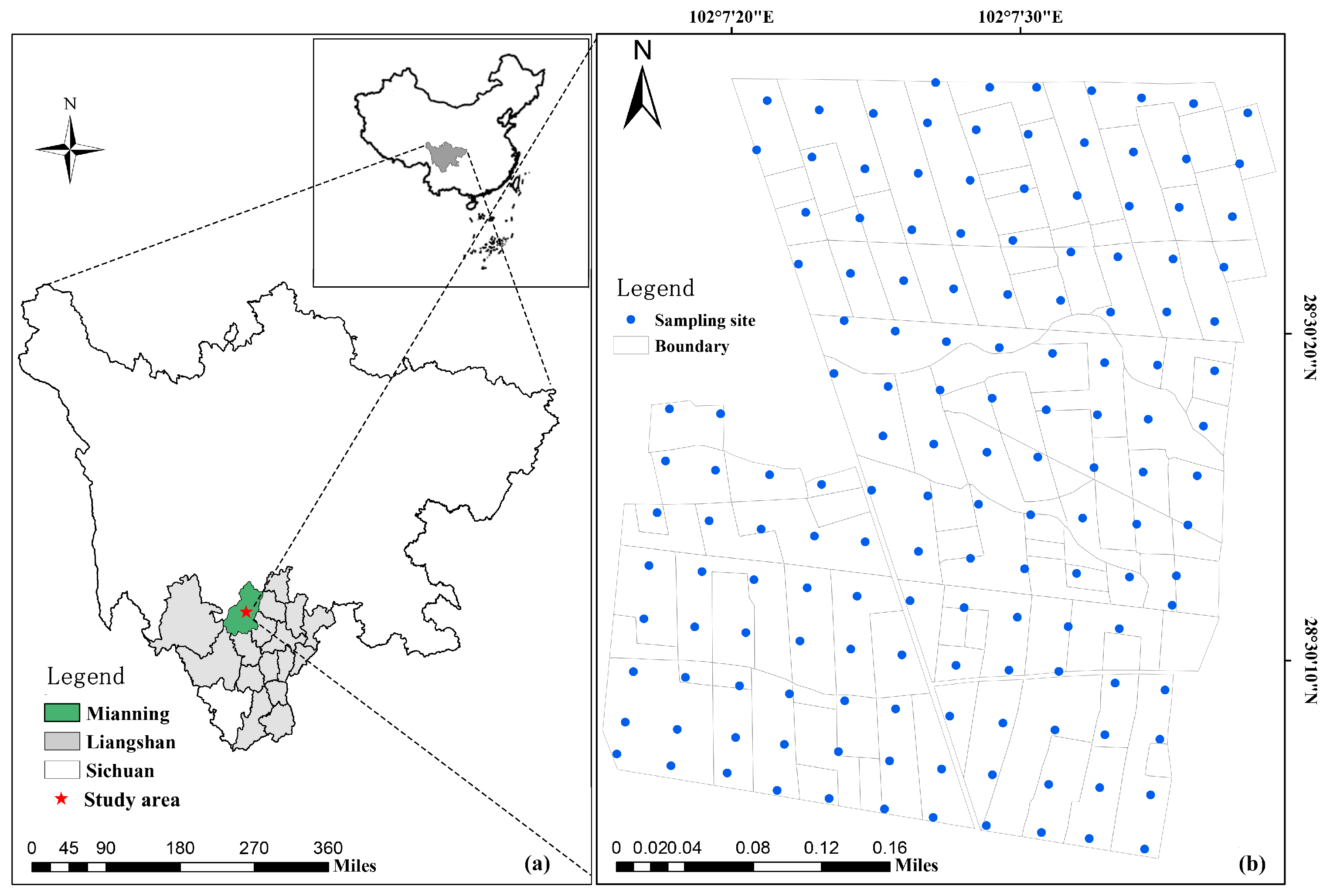
2.1. Study Area

The study area (28°30′3″–28°30′29″ N, 102°7′15″–102°7′41″ E) was located in Mianning County, Liangshan Yi Autonomous Prefecture, Sichuan Province, China. This area is characterized by relatively high terrain with an elevation of 1820 m. The area has a subtropical monsoon climate with an annual mean temperature and precipitation of approximately 14.5 °C and 1095 mm, respectively. The climate here is characterized by abundant sunshine, a high day–night temperature difference, and concentrated summer rainfall. The main soil types in the region are loam and clay loam (as described in the American system of soil texture classification) [34]. The region’s soil-forming parent material mainly consists of the mixture of red clay and alluvial matter and silt in the upstream of the Anning River, a tributary of Yalong River. The land use is cropland with corn, with buckwheat and flue-cured tobacco as the main crops. In this study, the WGS_1984_Albers projection coordinate system was used to produce the subset map (Figure 1).

2.2. Soil Sample Collection and Chemical Analysis

In October and November 2021, a total of 145 soil samples were collected at a 0–20 cm depth at 50 m × 50 m grid sampling points (Figure 1b). The study area covered a total area of approximately 35 ha, and the sampling points were distributed throughout the geographic range of the study area. Prior to the collection of each soil sample, a clear soil surface was selected with as little vegetation, grass and other disturbing substances as possible. Each soil sample was obtained using a composite of samples collected from five soil cores within a 5 m-radius circle at the square grid center. The geographic coordinates of each sampling point were recorded by a handheld global positioning instrument (GPS, 59222-C10, STONEX, Guangzhou, China) with a positioning error less than 10 m. After collection, rocks and plant residues in soil samples were removed, and the soil samples were taken to the laboratory, air-dried and sieved at 2 mm. Each sample was divided into two parts. One part was designated for standard chemical laboratory analysis and the other for spectrum data acquisition. The soil AK content was measured with the ammonium acetate extraction–flame photometric detection method and the titration of the AK extracts was performed with 1 mol L−1 NH4OAc with a 1:5 weight-to-volume ratio [35].

2.3. FITR Spectral Information Acquisition

The soil spectral reflectance was measured using a Bruker vertex 70v FTIR spectrometer (Bruker Corporation, Karlsruhe, Germany). The spectrometer’s data were digitized with a two-channel 24-bit delta-sigma ADC, and special OPUS software was used to control the spectrometer and record the Fourier transformation. The spectral data within the band range of 4000 to 400 cm−1 were recorded. The pretreated soil samples (the part used to reflect the spectrum) were ground, pulverized, and sieved through a 100-mesh screen to achieve a uniform surface for measurement. The soil sample (1 mg) and potassium bromide powder (99% purity, 200 mg) were ground in a 1:200 proportion using an agate mortar and then pressed into a 13 mm diameter disk with 112 bars of pressure for 2 min using a hydraulic press (L1272491, Perkin Elmer, Waltham, MA, USA). A blank KBr beam splitter was used to adjust to the baseline level prior to measurement. The background scan time and sample scan time were both 32 s, and the spectral resolution was 4 cm−1.

2.4. Dimension Reduction Algorithms

2.4.1. Successive Projections Algorithm (SPA)

The SPA is a positive characteristic variable selection method designed to find a representative set of spectral variables with a minimum of collinearity [36,37]. The principle of variable selection in the SPA is that among the remaining variables, the next variable selected should have the highest projected value onto the orthogonal subspace created by the previously selected variables. The maximum wavelength variable of the projection vector was selected as the candidate subset of the multiple linear regression (MLR) model, and the RMSE of the modeling dataset was obtained. Different RMSE values corresponded to different candidate subsets. The selection strategy of the SPA is to select the smallest RMSE [18,38]. In this study, the MinMaxScaler method was used to standardize the raw spectral data, and the ratio of the modeling set to the validation set was 3:1 during the SPA process.

2.4.2. Simulated Annealing Algorithm (SA)

The SA algorithm is a stochastic optimization algorithm, which can effectively avoid falling into a local minimum and eventually leads to a global optimum by giving the search process a time-varying probability jump that eventually tends toward zero [39,40]. Starting from a high initial temperature, the SA algorithm randomly searches for the global optimal solution of the objective function in the solution space with a certain probability jump characteristic as the temperature parameter continues to decrease, that is, the local optimal solution can jump out with probability and finally leads to the global optimum. The “certain probability” is calculated in reference to the annealing process of metal smelting, which is where the name of the simulated annealing algorithm comes from [41,42]. In this study, the root mean square error in cross-validation (RMSECV) was defined as the cost function and we sought to minimize it. The number of selected frequency bands and the definition of potential variables were based on many trial-and-error experiments. A total of 1000 iterations were performed, and the number of selected wavelengths was defined as 40.

2.4.3. Competitive Adaptive Reweighted Sampling (CARS)

CARS is a feature variable selection method combining the Monte Carlo sampling method and PLSR coefficient [43,44]. CARS is based on Darwin’s theory of evolution and follows the principle of “survival of the fittest” [45]. The band with a large absolute value of regression coefficients in the PLS model was selected by the adaptive reweighting sampling technique, and the band with a small weight was removed. Then, the lowest value of RMSECV was used to select the optimal variable subset and find the optimal variable combination. In this study, the number of variables selected was determined by 10 cross-validations, and the Monte Carlo sampling runs were set to 50.
The PLSR analysis is often used as a method to extract the latent variables (LVs) of the spectral data. These LVs can be utilized as a substitute for the original spectral data to reduce dimensionality, simplify the data, and explain the relationship between the spectral data and chemical constituents. Despite its potential benefits, PLSR has been found to be less effective than the above dimensionality reduction methods, particularly when working with high-dimensional FTIR data. In this paper, PLSR was adopted as the modeling approach and is described in detail in the following section.

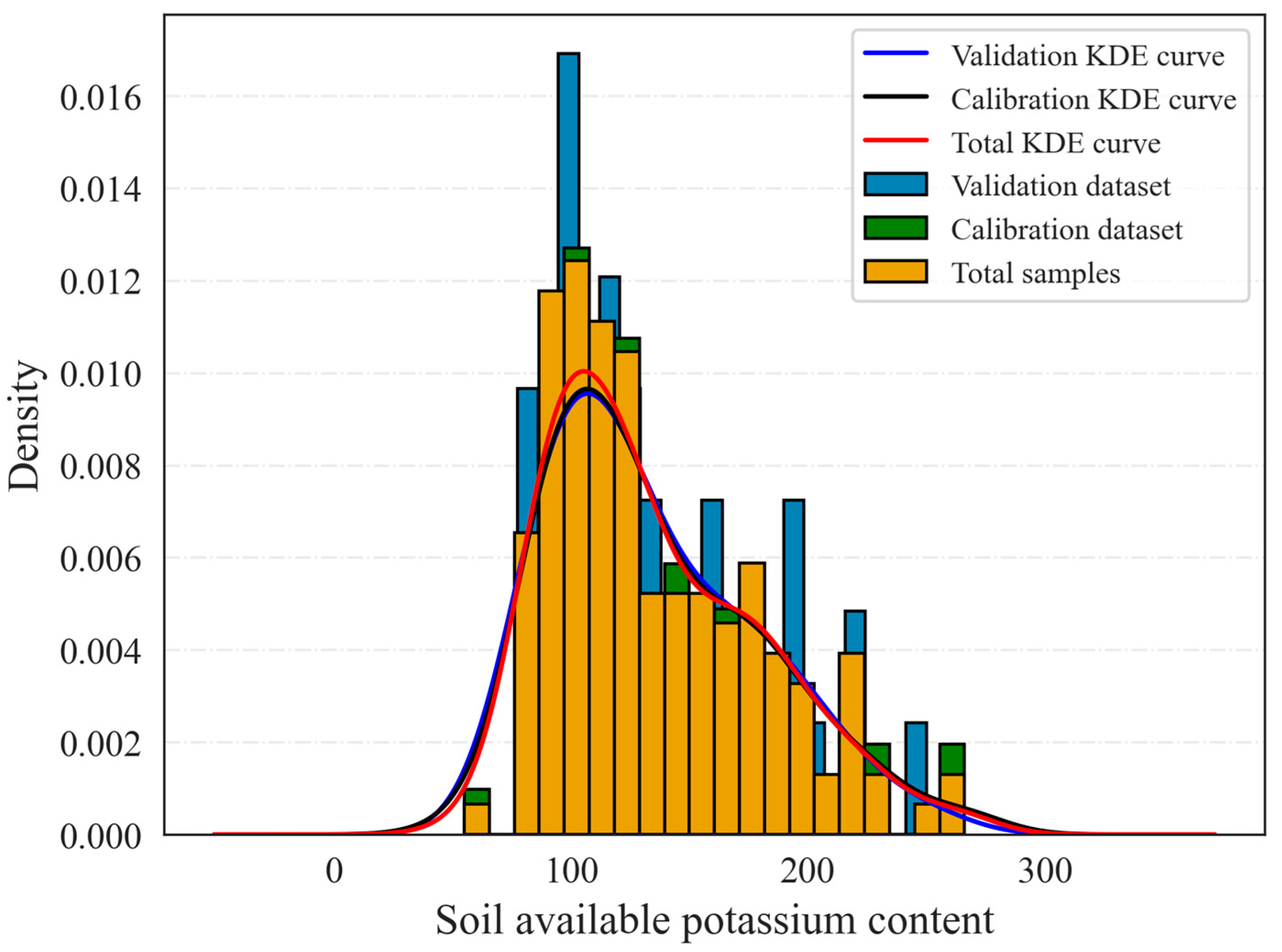
2.5. Dataset Partitioning

The 145 samples were divided into a calibration dataset (97 samples) and validation dataset (48 samples) using the hold-out method. The statistical information (kernel density estimation) of AK content in different datasets is shown in Figure 2.
The AK content in the whole dataset ranged from 55.00 mg/kg to 266.00 mg/kg, with a mean and CV of 134.98 mg/kg and 32.78%, respectively. The variability in AK content may be due to differences in soil conditions caused by diverse human cultivating practices and soil-forming environments. The means of the validation dataset and the calibration dataset were 135.48 mg/kg (SD = 45.15, CV = 31.97%) and 133.98 mg/kg (SD = 42.82, CV = 33.32%), respectively. There was no significant difference among the mean values of the whole dataset, calibration dataset and validation dataset (p > 0.05, T-test), and the probability distributions of soil AK ranges in different datasets were basically consistent. The calibration and validation datasets showed a skewed normal distribution as indicated by the kernel density curve, with kurtosis values of 0.134 and 0.126, and skewness values of 0.798 and 0.841, respectively, meeting the requirements of classical statistics [46].

2.6. Statistical Modeling and Accuracy Assessment

The partial least squares regression (PLSR) is the most commonly used multivariate statistical method, which is widely used in spectral data modeling and analysis [47]. The remarkable feature of the PLSR algorithm is that it considers the changes in independent variable space and dependent variable space simultaneously. By using finite factors to explain the change in independent variable space and dependent variable space, it can solve the serious autocorrelation problem between independent variables [48]. In this study, PLSR was performed according to sklearn.cross_decomposition in Python (version 3.9.1). The maximum number of principal components was set to 50, and then the optimal number of independent principal components (PCs) obtained by leave-one-out cross-validation (LOOCV) was used for variable selection. The PCs of RAW–PLSR, SPA–PLSR, SA–PLAR and CARS–PLSR inversion model are 10, 16, and 14, respectively.
Three assessment indexes were used to evaluate the accuracy of the soil AK content inversion model: coefficient of determination (R2), root mean square error (RMSE) and mean absolute value error (MAE). The corresponding formulas are given below:
R 2 = 1 i = 1 n ( y i ^ y ¯ ) 2 i = 1 n ( y i y ¯ ) 2
R M S E = 1 n i = 1 n ( y i y i ^ ) 2
M A E = 1 n i = 1 n | y i ^ y i |
where  n  is the number of soil samples and  y i  is the value of soil AK content detected by laboratory chemistry test (observed value).  y i ^  is the predicted value based on the inversion model.  y ¯    is the mean value of the observed value. In general, a well-performing model usually has a high R2 (close to 1) and a low RMSE and MAE (close to 0).

2.7. Contribution Analysis of Model Variables

To further understand the degree of relative importance of the variables (selected wavelength) in the inversion model, the contribution of the inversion model variables was explored. In this study, the scale function in sklearn.preprocessing in Python (version 3.9.1) was used to achieve data standardization and obtain the standardization coefficient of the inversion model. Based on this, the relative importance of the predictors of the PLSR model was calculated, which was used to further explain the relationship between soil AK content and different input variables. The formula for calculating the importance of variables (IV) is:
I V i = ( β i × 100 ) / β i ( i = 1 , 2 , 3 n )
where    β i  is the normalization coefficient of the inversion model.

3. Results

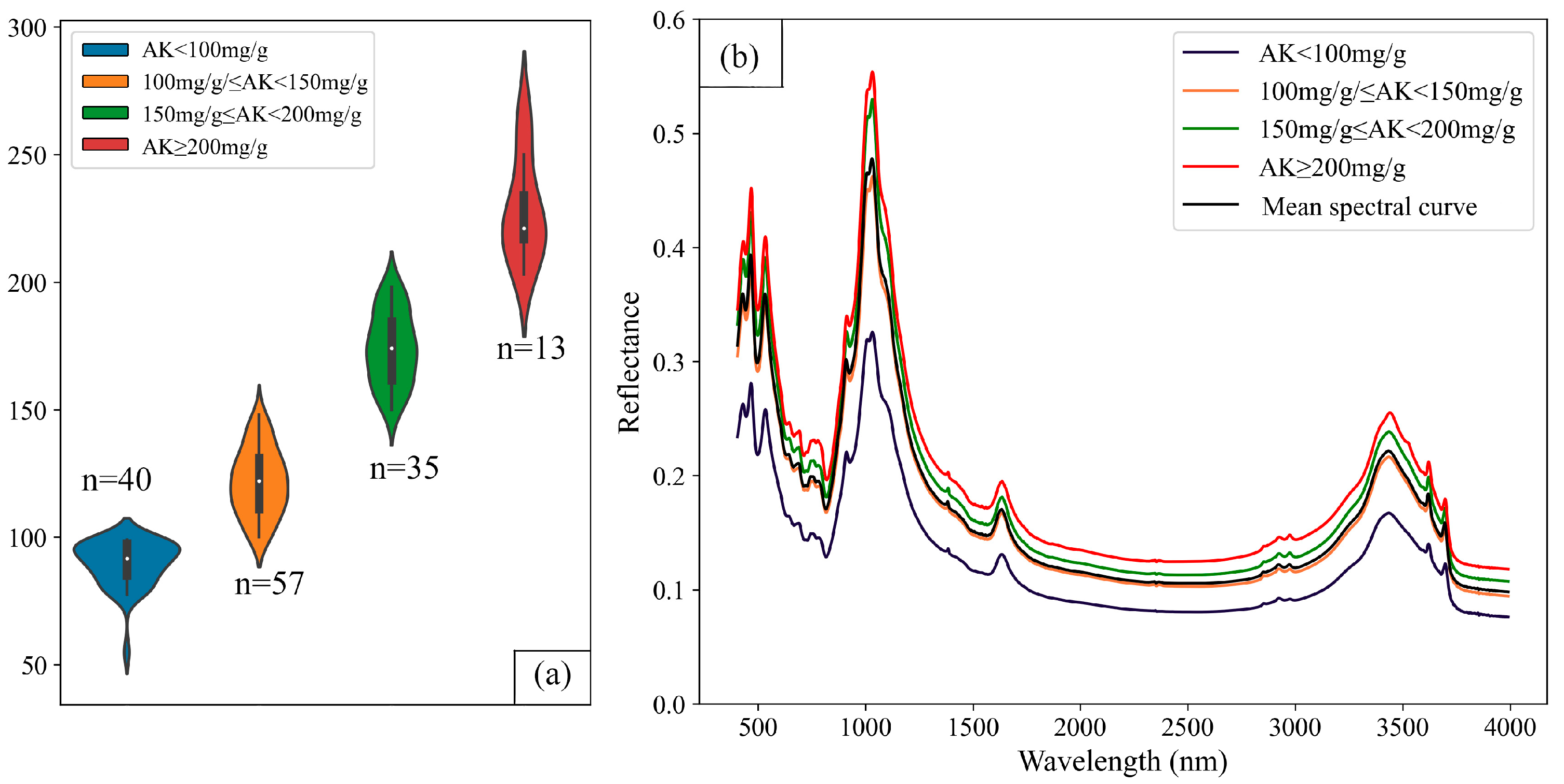
3.1. Description of Soil AK Content and FITR Characteristics

Based on the nutrient abundance and deficiency index of the China second soil survey [49] and the distribution of soil AK content in the study area, the AK content of the collected soil samples was divided into four different grade ranges: <100 mg/g (L1), [100, 150) mg/g (L2), [150, 200) mg/g (L3), ≥200 mg/g (L4) (Figure 3a). A total of 91% of the soil sample were under (≤) the soil AK content grade L3, and the number of soil samples of different grades was in the order of L2 (n = 57) > L1 (n = 40) > L3 (n = 35) > L4 (n = 13). In comparison to L4, the data distribution in L1, L2 and L3 was more centralized. Compared to the mean soil AK content (112.76 mg/g) of cropland in Sichuan province, China, the study area AK content was relatively high.
The variation trend of the average spectral reflectance of soil AK in different grades is shown in Figure 3b. Generally, with increasing soil AK content grade, the reflectance curve was relatively progressively enhanced. The spectral curve was relatively flat in the range of 1900 nm to 2800 nm. The main FTIR spectra reflectance peaks of the soil samples occurred at 453 nm, 537 nm, 1034 nm, 1638 nm and 3426 nm. Compared with other grades, the change trend of the mean spectral curve of all the soil samples was highly consistent with the [100, 150) mg/g grade.

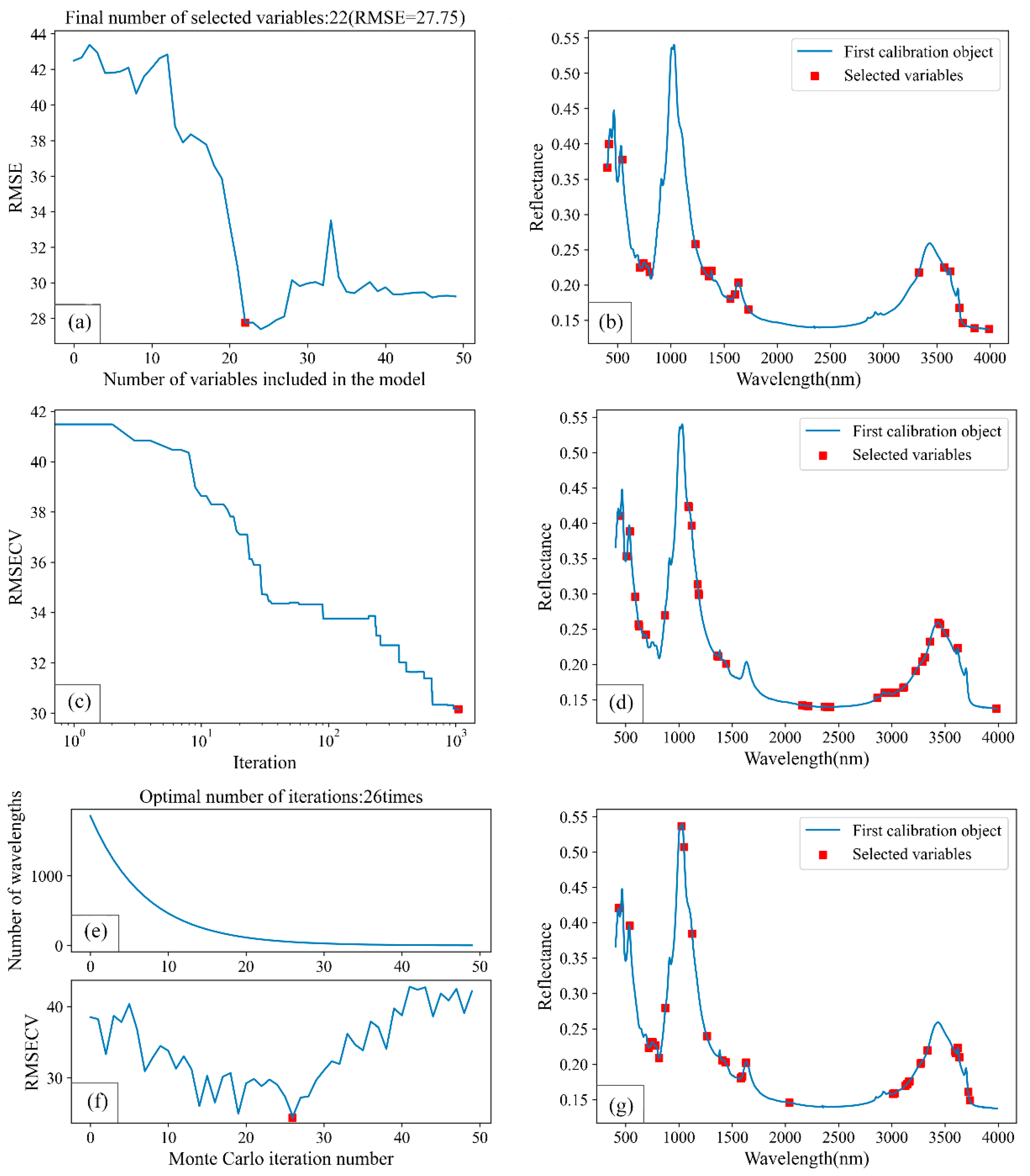
3.2. Dimensionality Reduction of Soil Spectral Data

In order to reduce the number of wavelengths in FTIR and obtain a simpler and more accurate inversion model, the SPA, SA and CARS were used to select the wavelengths related to AK content from the whole spectrum. The RMSE for the interactive verification of the modeling dataset in the SPA process demonstrated a pattern of initial decrease, followed by an increase, and finally stabilization (Figure 4a). When the number of variables was 22, the RMSE value dropped to 27.25 mg/g. Therefore, 22 characteristic wavelengths were selected as the dependent variables for the soil AK content inversion model based on the SPA. The distribution of the 22 characteristic wavelengths is shown in Figure 4b. The distribution is mainly concentrated in the ranges of 400–543 nm, 709–800 nm, 1230–1384 nm, 1558–1730 nm and 3330–3990 nm.
During the process of SA, the maximum value of the RMSECV of the modeling dataset is 41.53 mg/g; then is show gradually downward trend (Figure 4c). When the value of RMSECV drops to the lowest value of 40.32 mg/g, a total of 40 characteristic wavelengths were selected as the dependent variables to inversion model construction (Figure 4d). The distribution is denser in the ranges of 1359–1442 nm, 2158–2420 nm and 2864–3498 nm, and sparse in the range of 449–876 nm, 3618–3982 nm.
Figure 4e shows the change in the number of selected variables in the CARS algorithm. The number of selected variables decreased rapidly in the first 20 samples and then slowly, mainly due to the effect of the exponential decline function. A total of 49 variables were selected. Figure 4f shows the variation diagram of the RMSECV, which changed from high to low and then to high. When the number of sampling times was 26, the RMSECV reached the minimum value of 31.43 mg/g, which indicated that information variables unrelated to AK content were eliminated during the variable selection operation of 1–26 times. When the RMSECV rises beyond 26 times, key information variables related to the AK content may be eliminated, leading to an increase in the RMSECV value and the deterioration of the model effect. Figure 4g shows the distribution of the characteristic wavelengths. They are mainly distributed at 715–873 nm, 1024–1263 nm, 1406–1629 nm, 3012–3334 nm and 3595–3732 nm.

3.3. The Results of Different Inversion Models

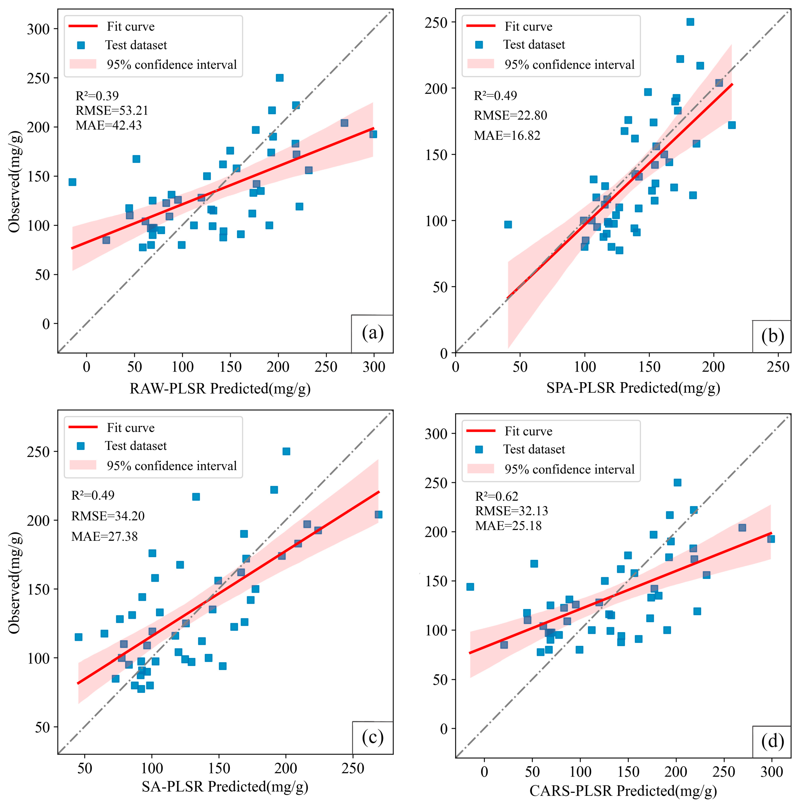
3.3.1. Model Performances of Different Dimensionality Reduction Methods

The characteristic wavelengths extracted by the SPA, SA and CARS algorithms and the raw spectral data were combined with PLSR for soil AK inversion model construction. The validation dataset was used to build the inversion model, and the calibration dataset was used to inspect the robustness and accuracy of the model, then to choose the best dimensionality reduction and PLSR combination.
The accuracy of the soil AK content inversion model for different combinations of dimensionality reduction and PLSR is shown in (Figure 5) The orders of R2, RMSE and MAE for different combinations are CARS–PLSR (0.62) > SA–PLSR (0.49) = SPA–PLSR (0.49) > RAW–PLSR (0.39), RAW–PLSR (55.21) > CARS–PLSR (32.13) > SA–PLSR (34.2) > SPA–PLSR (22.8) and RAW–PLSR (42.43) > SA–PLSR (27.38) > CARS–PLSR (25.18) > SPA--PLSR (16.82), respectively. The results demonstrated that after spectral dimensionality reduction, inversion-model-simplified spectral wavelengths showed better performance with higher R2 and lower RMSE and MAE values than their corresponding raw-spectrum inversion models for AK content estimation, which indicated that the variable selection produced more effective models with a simplified model. Overall, the soil AK content inversion model constructed by the SPA dimensional reduction had the best performance, the SPA–PLSR model’s RMSE and MAE were the smallest, and the model’s R2 was the second largest after CARS–PLSR.

3.3.2. Contribution of Variables Using Different Inversion Models

The variable relative importance derived from SPA–PLSR inversion models is displayed in Figure 6. This figure identifies which spectral variables are the most important predictors in the spectral estimation of AK content. For RAW–PLSR, the FTIR data without dimensionality reduction, a total of 1860 wavelengths were involved in the modeling, and the contribution of each variable was low (<0.37%), which means that informational wavelengths were not selected for the quantitative estimation of soil AK content when directly using the full spectrum as an input variable. The SPA–PLSR model was the model with the best inversion result (Figure 5). According to the calculation of the SPA, a total of 22 characteristic wavelengths were selected as input variables of PLSR, and the top 10 characteristic wavelengths with the largest contributions were mainly distributed in the near-infrared region: 1635 nm (11.96%) > 1315 nm (7.59%) > 777 nm (5.43%) > 1730 nm (5.03%) > 1357 nm (5.01%) and the middle-infrared region: 3568 nm (8.8%) > 3855 nm (8.03%) > 3990 nm (6.68%) > 3626 nm (5.70%) > 3712 nm (4.91%). For all the characteristic wavelength selected by SPA, there was a significant correlation between the wavelength and soil AK content (Pearson correlation, p < 0.01).

4. Discussion

4.1. Comparison of Dimensionality Reduction Algorithms

The raw spectral information generally contains a large amount of redundant information, and the accuracy of the model is not good when used to directly construct predictions of soil properties, so feature extraction from a large number of spectra is crucial [50,51]. The use of dimensionality reduction is a powerful tool to improve the potential of spectroscopy, which can not only extract the effective information of the raw spectral curve, but also effectively solve the multicollinearity problem between spectral wavelengths [52]. Figure 5 shows that in light of the inversion model of dimensionality reduction data as independent variables, FTIR provided relatively satisfactory results for estimating AK content in the study area. In order to further compare the differences between the three dimensionality reduction methods, the variable initialization, evaluation indicators and selection strategies of the three algorithms SPA, SA and CARS are summarized in Table 1.
In the process of the dimensionality reduction of spectral variables, each wavelength is regarded as a unit (i.e., a variable). The selected variables are thus discrete. There are two ways to initialize variables: all the variables and a part of the variable. The SPA considers all variables to initialize, and then employs simple projection operations in a vector space and the forward selection method to obtain subsets of variables with a minimum collinearity [53]. Figure 5 shows that the SPA is an advantageous approach in analyzing reflectance spectra, and the results of its inversion model were superior to the SA algorithm and CARS algorithm. Vibhute et al. [54] reported that the SPA is a valuable tool for estimating soil properties with diffuse reflectance in NIR spectroscopy. Shi et al. [55] indicated that the SPA is simpler and more time-saving compared with the GA in selecting the spectral characteristic wavelengths of SOM prediction. Our findings are consistent with these above reports. Guo et al. [18] employed a combination of two variable selection methods (CARS and SPA) in a regression algorithm to predict soil nutrients (N, P, K), and their results showed that CARS was more effective than the SPA. This conclusion is contrary to the conclusion of our study. The difference in results could be due to several factors. Firstly, Guo et al. preprocessed the original spectral information (multiplicative scatter correction (MSC) and standard normalized variate (SNV)) before applying the variable selection methods, whereas this was not performed in our study. This preprocessing step can affect the outcome of the variable selection. Secondly, the spectral data used in our study were obtained using FTIR with a high resolution of 4 cm−1, resulting in 1860 spectral variables, which can introduce noise and interference. The SPA may perform better in high-dimensional data reduction as it prioritizes useful information, reduces variable covariance and minimizes the linear relationship between variables [36,37,38]. Additionally, differences in soil properties in different areas, including soil moisture content, soil texture, and soil color, could also contribute to differences in research outcomes [56].
The SA and CARS algorithms adopt the random sampling and Monte Carlo sampling methods, respectively, to select initial variables. That is, the SA and CARS algorithms use a part of the variable as the initial variable. The characteristic of the SA algorithm is robust, high computational efficiency, and it easily falls into local optimization [57]. In this study, the performance of the SA algorithm was second only to the SPA. CARS uses the largest absolute regression coefficients as the evaluation metric and the exponentially decreasing function (EDF) as a selection strategy to competitively select characteristic variables based on adaptive reweighted sampling [58]. The poor performance of CARS in this study may have been due to the collinearity of the selected characteristic wavelength. Some scholars have shown that the characteristic wavelength selected by CARS usually contains collinear variables [59,60,61], and other dimension reduction algorithms are needed to further extract collinear variables to obtain the combination of minimum collinear wavelength variables.

4.2. Soil Available Potassium Characteristic Wavelengths

Soil spectral reflectance is affected by its physical properties, chemical composition, and mineral composition [62]. At the microscopic level, the outer electrons of ions or the chemical bands of different molecules vibrate at characteristic frequencies under the action of electromagnetic energy [63]. In this process, there are steps of reflection, absorption, and scattering of electromagnetic energy, which may have a direct correlation with the spectral curve. Therefore, the interpretation of the spectra of soil samples can aid in understanding the soil nutrient content information.
The results of the variable contribution analysis indicated that the significant wavelengths for soil AK content were located around 777 nm, 1315 nm, 1375 nm, 1635 nm, 1730 nm and 3568–3990 nm. These results are in agreement with previous research that identified the key wavelengths related to the 2:1 clay mineral, which primarily fell around 1400 nm and 1900 nm [64,65]. The spectral response of cations (such as K+ and Mg2+) in soil is similar to the sensitivity zone of clay minerals, such as kaolinite and montmorillonite, which provide the CEC, as demonstrated by Dematte et al. [66] and supported by Barré et al. [67] and Velde et al. [68]. However, it should be noted that the results of this study were based on in situ soil sampling and may differ from studies conducted in different regions. For example, Guo et al. [18] found that the most common characteristic wavelengths for AK in paddy soil were located around 400–483 nm, 728 nm, 967–1031 nm, 1271–1409 nm, 1643–1789 nm, 1975–2004 nm, 2109–2174 nm, and 2312–2449 nm. The differences in soil AK characteristic wavelengths across different regions can be attributed to factors such as soil heterogeneity, moisture content, texture, color, sample number, sample and spectral data pretreatment, concentration range, and the model development method [17,25,69].

4.3. Limitation and Uncertainty

Spectral dimensionality reductions are an integral component of the spectroscopist’s toolbox, and in soil science there is a suite of applications that improve or enable the characterization of soil components and processes. In this study, three dimensionality reduction algorithms were used to explore the response of soil AK content to FTIR, and an inversion model of soil AK content was established. Although different dimensionality reduction and PLSR regression combinations were applied in this study, there are still many limitations in the application of the algorithms presented in this paper. The default parameters were used in all the adopted methods, and no parameters were chosen for optimization. In addition, only the PLS algorithm was used in the modeling, without comparing the various modeling methods, which generally leads to algorithmic uncertainty. Another source of uncertainty may have arisen from the choice of soil sampling strategy. In this study, only a limited area was selected for sampling. Although it could represent the characteristics of local farmland, based on soil sampling data, it was not adequate to build a universal inversion model of soil AK content. In addition, environmental factors are commonly crucial to the inversion of soil AK content [21,69], and the relationships among environmental factors, spectral data and inversion models were not thoroughly discussed in this paper.
In future studies, the inversion model for estimating soil AK content can be improved in several ways. First, a more consistent and standardized soil sampling strategy should be implemented to reduce the uncertainty introduced by variations in topography and tillage methods. Second, a comparison of different machine-learning algorithms and their performance in terms of feature extraction and the modeling of spectral data should be conducted to improve the accuracy of the inversion model. Finally, the development of portable and user-friendly field spectral equipment that can be easily integrated with environmental data would enable the use of the inversion model on a larger scale.

5. Conclusions

This study measured the FTIR spectra of 145 soil sample sites in in Mianning County, Liangshan Yi Autonomous Prefecture, Sichuan Province, China. To reveal the relationship between the soil FTIR spectral information and soil AK content, the PLSR method combined with three dimensionality reduction methods (SPA, SA and CARS) was used to estimate the soil AK content. The results illustrate that the inversion model performance could be significantly improved by applying proper spectral dimensionality reduction methods, and the details for this are as follows:
(1)
The application of the dimensionality reduction method can effectively limit the correlation between adjacent frequency bands, reduce data redundancy, and improve inversion modeling accuracy to a certain extent. Compared with the SA and CARS algorithms, the SPA was more suitable for spectral dimension reduction of soil AK content prediction.
(2)
The results show that the characteristic wavelengths were mainly around 777 nm, 1315 nm, 1375 nm, 1635 nm, 1730 nm and 3568–3990 nm.
(3)
Compared the performance of different soil AK inversion models, the SPA–PLSR model (R2 = 0.49, RMSE = 22.80, MAE = 16.82) was superior to the SA–PLSR and CARS–PLSR models, which has certain guiding significance for the rapid detection of soil AK content.

Author Contributions

Conceptualization, W.W. and Y.Z.; Methodology, W.W. and N.C.; Software, W.W.; Validation, Z.L., Y.Z. and N.C.; Formal analysis, W.W. and N.C.; Investigation, W.W., Y.Z. and H.J.; Resources, Y.C.; Writing—original draft preparation, W.W.; Writing—review and editing, W.W. and N.C.; Visualization, Q.L.; Supervision, N.C. and W.F.; Project administration, H.L.; All authors have read and agreed to the published version of the manuscript.

Funding

This study was supported by The Agricultural Science and Technology Foundation of Sichuan Province, China (SCYC202005).

Institutional Review Board Statement

Not applicable.

Informed Consent Statement

Not applicable.

Data Availability Statement

The data presented in this study are available on request from the corresponding author. The data are not publicly available due to the project requirements.

Conflicts of Interest

The authors declare no conflict of interest.

References

  1. Azzawi, W.A.; Gill, M.B.; Fatehi, F.; Zhou, M.; Acuña, T.; Shabala, L.; Yu, M.; Shabala, S. Effects of potassium availability on growth and development of barley cultivars. Agronomy 2021, 11, 2269. [Google Scholar] [CrossRef]
  2. Rawat, J.; Sanwal, P.; Saxena, J. Potassium and its role in sustainable agriculture. In Potassium Solubilizing Microorganisms for Sustainable Agriculture; Springer: New Delhi, India, 2016; p. 253. [Google Scholar]
  3. Römheld, V.; Kirkby, E.A. Research on potassium in agriculture: Needs and prospects. Plant Soil 2010, 335, 155–180. [Google Scholar] [CrossRef]
  4. Chen, Q.; Xin, Y.; Liu, Z. Long-term fertilization with potassium modifies soil biological quality in K-rich soils. Agronomy 2020, 10, 771. [Google Scholar] [CrossRef]
  5. Alomar, S.; Mireei, S.A.; Hemmat, A.; Masoumi, A.; Khademi, H. Comparison of Vis/SWNIR and NIR spectrometers combined with different multivariate techniques for estimating soil fertility parameters of calcareous topsoil in an arid climate. Biosyst. Eng. 2021, 201, 50–66. [Google Scholar] [CrossRef]
  6. Li, H.; Wang, J.; Zhang, J.; Liu, T.; Acquah, G.E.; Yuan, H. Combining Variable Selection and Multiple Linear Regression for Soil Organic Matter and Total Nitrogen Estimation by DRIFT-MIR Spectroscopy. Agronomy 2022, 12, 638. [Google Scholar] [CrossRef]
  7. Munawar, A.A. Rapid and simultaneous detection of hazardous heavy metals contamination in agricultural soil using infrared reflectance spectroscopy. In IOP Conference Series: Materials Science and Engineering; IOP Publishing: Bristol, UK, 2019; Volume 506, p. 012008. [Google Scholar]
  8. Cécillon, L.; Barthès, B.G.; Gomez, C.; Ertlen, D.; Genot, V.; Hedde, M.; Stevens, A.; Brun, J.J. Assessment and monitoring of soil quality using near-infrared reflectance spectroscopy (NIRS). Eur. J. Soil Sci. 2009, 60, 770–784. [Google Scholar] [CrossRef] [Green Version]
  9. Petit, T.; Puskar, L. FTIR spectroscopy of nanodiamonds: Methods and interpretation. Diam. Relat. Mater. 2018, 89, 52–66. [Google Scholar] [CrossRef]
  10. López-Lorente, Á.I.; Mizaikoff, B. Recent advances on the characterization of nanoparticles using infrared spectroscopy. TrAC Trends Anal. Chem. 2016, 84, 97–106. [Google Scholar] [CrossRef]
  11. Mudunkotuwa, I.A.; Al Minshid, A.; Grassian, V.H. ATR-FTIR spectroscopy as a tool to probe surface adsorption on nanoparticles at the liquid–solid interface in environmentally and biologically relevant media. Analyst 2014, 139, 870–881. [Google Scholar] [CrossRef]
  12. Tinti, A.; Tugnoli, V.; Bonora, S.; Francioso, O. Recent applications of vibrational mid-Infrared (IR) spectroscopy for studying soil components: A review. J. Cent. Eur. Agric. 2015, 16, 1–22. [Google Scholar] [CrossRef]
  13. Sørensen, L.K.; Dalsgaard, S. Determination of clay and other soil properties by near infrared spectroscopy. Soil Sci. Soc. Am. J. 2005, 69, 159–167. [Google Scholar] [CrossRef]
  14. Singh, P.; Singh, M.K.; Beg, Y.R.; Nishad, G.K. A review on spectroscopic methods for determination of nitrite and nitrate in environmental samples. Talanta 2019, 191, 364–381. [Google Scholar] [CrossRef] [PubMed]
  15. Xing, Z.; Du, C.; Shen, Y.; Ma, F.; Zhou, J. A method combining FTIR-ATR and Raman spectroscopy to determine soil organic matter: Improvement of prediction accuracy using competitive adaptive reweighted sampling (CARS). Comput. Electron. Agric. 2021, 191, 106549. [Google Scholar] [CrossRef]
  16. Jahn, B.R.; Linker, R.; Upadhyaya, S.K.; Shaviv, A.; Slaughter, D.C.; Shmulevich, I. Mid-infrared spectroscopic determination of soil nitrate content. Biosyst. Eng. 2006, 94, 505–515. [Google Scholar] [CrossRef]
  17. Stenberg, B.; Rossel, R.A.V.; Mouazen, A.M.; Wetterlind, J. Visible and near infrared spectroscopy in soil science. Adv. Agron. 2010, 107, 163–215. [Google Scholar]
  18. Guo, P.; Li, T.; Gao, H.; Chen, X.; Cui, Y.; Huang, Y. Evaluating calibration and spectral variable selection methods for predicting three soil nutrients using Vis-NIR spectroscopy. Remote Sens. 2021, 13, 4000. [Google Scholar] [CrossRef]
  19. Veum, K.S.; Sudduth, K.A.; Kremer, R.J.; Kitchen, N.R. Estimating a soil quality index with VNIR reflectance spectroscopy. Soil Sci. Soc. Am. J. 2015, 79, 637–649. [Google Scholar] [CrossRef]
  20. Xia, Y.; Ugarte, C.M.; Guan, K.; Pentrak, M.; Wander, M.M. Developing near-and mid-infrared spectroscopy analysis methods for rapid assessment of soil quality in Illinois. Soil Sci. Soc. Am. J. 2018, 82, 1415–1427. [Google Scholar] [CrossRef] [Green Version]
  21. Kinoshita, R.; Moebius-Clune, B.N.; van Es, H.M.; Hively, W.D.; Bilgilis, A.V. Strategies for soil quality assessment using visible and near-infrared reflectance spectroscopy in a Western Kenya chronosequence. Soil Sci. Soc. Am. J. 2012, 76, 1776–1788. [Google Scholar] [CrossRef] [Green Version]
  22. Margenot, A.J.; Calderón, F.J.; Parikh, S.J. Limitations and potential of spectral subtractions in Fourier-transform infrared spectroscopy of soil samples. Soil Sci. Soc. Am. J. 2016, 80, 10–26. [Google Scholar] [CrossRef] [Green Version]
  23. Angelopoulou, T.; Tziolas, N.; Balafoutis, A.; Zalidis, G.; Bochtis, D. Remote sensing techniques for soil organic carbon estimation: A review. Remote Sens. 2019, 11, 676. [Google Scholar] [CrossRef] [Green Version]
  24. Pullanagari, R.R.; Kereszturi, G.; Yule, I. Integrating airborne hyperspectral, topographic, and soil data for estimating pasture quality using recursive feature elimination with random forest regression. Remote Sens. 2018, 10, 1117. [Google Scholar] [CrossRef] [Green Version]
  25. Xu, L.; Schechter, I. Wavelength selection for simultaneous spectroscopic analysis. Experimental and theoretical study. Anal. Chem. 1996, 68, 2392–2400. [Google Scholar] [CrossRef]
  26. Schreier, H. Quantitative Predictions of Chemical Soil Conditions from Multispectral Airborne Ground and Laboratory Measurements. Pascal Fr. Bibliogr. Databases 1977, 106–112. [Google Scholar]
  27. Araújo, M.C.U.; Saldanha, T.C.B.; Galvao, R.K.H.; Yoneyama, T.; Chame, H.C.; Visani, V. The successive projections algorithm for variable selection in spectroscopic multicomponent analysis. Chemom. Intell. Lab. Syst. 2001, 57, 65–73. [Google Scholar] [CrossRef]
  28. Chong, I.G.; Jun, C.H. Performance of some variable selection methods when multicollinearity is present. Chemom. Intell. Lab. Syst. 2005, 78, 103–112. [Google Scholar] [CrossRef]
  29. Cai, W.; Li, Y.; Shao, X. A variable selection method based on uninformative variable elimination for multivariate calibration of near-infrared spectra. Chemom. Intell. Lab. Syst. 2008, 90, 188–194. [Google Scholar] [CrossRef]
  30. Meerts, W.L.; Schmitt, M.; Groenenboom, G.C. New applications of the genetic algorithm for the interpretation of high-resolution spectra. Can. J. Chem. 2004, 82, 804–819. [Google Scholar] [CrossRef] [Green Version]
  31. Jia, S.; Yang, X.; Zhang, J.; Li, G. Quantitative analysis of soil nitrogen, organic carbon, available phosphorous, and available potassium using near-infrared spectroscopy combined with variable selection. Soil Sci. 2014, 179, 211–219. [Google Scholar] [CrossRef]
  32. Peng, Y.; Zhao, L.; Hu, Y.; Wang, G.; Wang, L.; Liu, Z. Prediction of soil nutrient contents using visible and near-infrared reflectance spectroscopy. ISPRS Int. J. Geo-Inf. 2019, 8, 437. [Google Scholar] [CrossRef] [Green Version]
  33. Xu, D.; Zhao, R.; Li, S.; Chen, S.; Jiang, Q.; Zhou, L.; Shi, Z. Multi-sensor fusion for the determination of several soil properties in the Yangtze River Delta, China. Eur. J. Soil Sci. 2019, 70, 162–173. [Google Scholar] [CrossRef] [Green Version]
  34. Kyebogola, S.; Burras, L.C.; Miller, B.A.; Semalulu, O.; Yost, R.S.; Tenywa, M.M.; Lenssen, A.W.; Kyomuhendo, P.; Smith, C.; Luswata, C.K.; et al. Comparing Uganda’s indigenous soil classification system with World Reference Base and USDA Soil Taxonomy to predict soil productivity. Geoderma Reg. 2020, 22, e00296. [Google Scholar] [CrossRef]
  35. Bao, S.D. Soil and Agricultural Chemistry Snalysis; China Agricultural Press: Beijing, China, 1981. [Google Scholar]
  36. Zhang, H.L.; Wei, L.; Liu, X.M.; He, Y. SPA on spectral multivariable selection with different calibration methods for the determination of soil total nitrogen content. Int. Agric. Eng. J. 2017, 26, 9–15. [Google Scholar]
  37. Maraphum, K.; Ounkaew, A.; Kasemsiri, P.; Hiziroglu, S.; Posom, J. Wavelengths selection based on genetic algorithm (GA) and successive projections algorithms (SPA) combine with PLS regression for determination the soluble solids content in Nam-DokMai mangoes based on near infrared spectroscopy. Eng. Appl. Sci. Res. 2022, 49, 119–126. [Google Scholar]
  38. Luo, W.; Fan, G.; Tian, P.; Dong, W.; Zhang, H.; Zhan, B. Spectrum classification of citrus tissues infected by fungi and multispectral image identification of early rotten oranges. Spectrochim. Acta Part A Mol. Biomol. Spectrosc. 2022, 279, 121412. [Google Scholar] [CrossRef] [PubMed]
  39. Delahaye, D.; Chaimatanan, S.; Mongeau, M. Simulated annealing: From basics to applications. In Handbook of Metaheuristics; Springer: Cham, Switzerland, 2019; pp. 1–35. [Google Scholar]
  40. Kirkpatrick, S.; Gelatt, C.; Vecchi, M. Simulated annealing methods. J. Stat. Phys. 1984, 34, 975. [Google Scholar] [CrossRef]
  41. Hörchner, U.; Kalivas, J.H. Further investigation on a comparative study of simulated annealing and genetic algorithm for wavelength selection. Anal. Chim. Acta 1995, 311, 1–13. [Google Scholar] [CrossRef]
  42. Ballabio, C.; Panagos, P.; Lugato, E.; Huang, J.-H.; Orgiazzi, A.; Jones, A.; Fernández-Ugalde, O.; Borrelli, P.; Montanarella, L. Copper distribution in European topsoils: An assessment based on LUCAS soil survey. Sci. Total Environ. 2018, 636, 282–298. [Google Scholar] [CrossRef]
  43. Druet, S.A.J.; Taran, J.P.E. CARS spectroscopy. Prog. Quantum Electron. 1981, 7, 1–72. [Google Scholar] [CrossRef]
  44. Wang, C.; Li, X.; Wang, L.; Yang, C.; Chen, X.; Li, M.; Ma, S. Prediction of N, P, and K Contents in Sugarcane Leaves by VIS-NIR Spectroscopy and Modeling of NPK Interaction Effects. Trans. ASABE 2019, 62, 1427–1433. [Google Scholar] [CrossRef]
  45. Liu, J.; Dong, Z.; Xia, J.; Wang, H.; Meng, T.; Zhang, R.; Han, J.; Wang, N.; Xie, J. Estimation of soil organic matter content based on CARS algorithm coupled with random forest. Spectrochim. Acta Part A: Mol. Biomol. Spectrosc. 2021, 258, 119823. [Google Scholar] [CrossRef] [PubMed]
  46. Efron, B.; Tibshirani, R. Statistical data analysis in the computer age. Science 1991, 253, 390–395. [Google Scholar] [CrossRef] [PubMed] [Green Version]
  47. Xie, J.; Pan, Q.; Li, F.; Tang, Y.; Hou, S.; Xu, C. Simultaneous detection of trace adulterants in food based on multi-molecular infrared (MM-IR) spectroscopy. Talanta 2021, 222, 121325. [Google Scholar] [CrossRef]
  48. Peng, Z.; Guan, L.; Liao, Y.; Lian, S. Estimating total leaf chlorophyll content of gannan navel orange leaves using hyperspectral data based on partial least squares regression. IEEE Access 2019, 7, 155540–155551. [Google Scholar] [CrossRef]
  49. Teng, Y.; Wu, J.; Lu, S.; Wang, Y.; Jiao, X.; Song, L. Soil and soil environmental quality monitoring in China: A review. Environ. Int. 2014, 69, 177–199. [Google Scholar] [CrossRef]
  50. Linker, R.; Shmulevich, I.; Kenny, A.; Shaviv, A. Soil identification and chemometrics for direct determination of nitrate in soils using FTIR-ATR mid-infrared spectroscopy. Chemosphere 2005, 61, 652–658. [Google Scholar] [CrossRef]
  51. Shaviv, A.; Kenny, A.; Shmulevich, I.; Singher, L.; Reichlin, Y.; Katzir, A. IR fiberoptic systems for in situ and real time monitoring of nitrate in water and environmental systems. Environ. Sci. Technol. 2003, 37, 2807–2812. [Google Scholar] [CrossRef] [PubMed]
  52. Erny, G.L.; Brito, E.; Pereira, A.B.; Bento-Silva, A.; Patto, M.C.V.; Bronze, M.R. Projection to latent correlative structures, a dimension reduction strategy for spectral-based classification. RSC Adv. 2021, 11, 29124–29129. [Google Scholar] [CrossRef]
  53. Yun, Y.H.; Li, H.D.; Deng, B.C.; Cao, D.S. An overview of variable selection methods in multivariate analysis of near-infrared spectra. TrAC Trends Anal. Chem. 2019, 113, 102–115. [Google Scholar] [CrossRef]
  54. Vibhute, A.D.; Kale, K.V.; Mehrotra, S.C.; Dhumal, R.K.; Nagne, A.D. Determination of soil physicochemical attributes in farming sites through visible, near-infrared diffuse reflectance spectroscopy and PLSR modeling. Ecol. Process. 2018, 7, 26 . [Google Scholar] [CrossRef] [Green Version]
  55. Shi, T.; Chen, Y.; Liu, H.; Wang, J.; Wu, G. Soil organic carbon content estimation with laboratory-based visible-near-infrared reflectance spectroscopy: Feature selection. Appl. Spectrosc. 2014, 68, 831–837. [Google Scholar] [CrossRef]
  56. Yang, X. An extension to “Mid-infrared spectral interpretation of soils: Is it practical or accurate?”. Geoderma 2014, 226, 415–417. [Google Scholar] [CrossRef]
  57. Rutenbar, R.A. Simulated annealing algorithms: An overview. IEEE Circuits Devices Mag. 1989, 5, 19–26. [Google Scholar] [CrossRef]
  58. Tolles, W.M.; Nibler, J.W.; McDonald, J.R.; Harvey, A.B. A review of the theory and application of coherent anti-Stokes Raman spectroscopy (CARS). Appl. Spectrosc. 1977, 31, 253–271. [Google Scholar] [CrossRef]
  59. Zhang, D.; Xu, Y.; Huang, W.; Tian, X.; Xia, Y.; Xu, L.; Fan, S. Nondestructive measurement of soluble solids content in apple using near infrared hyperspectral imaging coupled with wavelength selection algorithm. Infrared Phys. Technol. 2019, 98, 297–304. [Google Scholar] [CrossRef]
  60. Wang, Z.; Wang, X.; Zhong, G.; Liu, J.; Sun, Y.; Zhang, C. Rapid determination of ammonia nitrogen concentration in biogas slurry based on NIR transmission spectroscopy with characteristic wavelength selection. Infrared Phys. Technol. 2022, 122, 104085. [Google Scholar] [CrossRef]
  61. Xiao, S.; He, Y.; Dong, T.; Nie, P. Spectral analysis and sensitive waveband determination based on nitrogen detection of different soil types using near infrared sensors. Sensors 2018, 18, 523. [Google Scholar] [CrossRef] [PubMed] [Green Version]
  62. Katuwal, S.; Knadel, M.; Moldrup, P.; Norgaard, T.; Greve, M.H.; de Jonge, L.W. Visible–Near-infrared spectroscopy can predict mass transport of dissolved chemicals through intact soil. Sci. Rep. 2018, 8, 11188. [Google Scholar] [CrossRef] [Green Version]
  63. Kawamura, K.; Tsujimoto, Y.; Nishigaki, T.; Andriamananjara, A.; Rabenarivo, M.; Asai, H.; Rakotoson, T.; Razafimbelo, T. Laboratory visible and near-infrared spectroscopy with genetic algorithm-based partial least squares regression for assessing the soil phosphorus content of upland and lowland rice fields in Madagascar. Remote Sens. 2019, 11, 506. [Google Scholar] [CrossRef] [Green Version]
  64. Dematte, J.A.M.; Garcia, G.J. Alteration of soil properties through a weathering sequence as evaluated by spectral reflectance. Soil Sci. Soc. Am. J. 1999, 63, 327–342. [Google Scholar] [CrossRef]
  65. Goetz, A.F.H.; Curtiss, B.; Shiley, D.A. Rapid gangue mineral concentration measurement over conveyors by NIR reflectance spectroscopy. Miner. Eng. 2009, 22, 490–499. [Google Scholar] [CrossRef]
  66. Demattê, J.A.M.; Ramirez-Lopez, L.; Marques, K.P.P.; Rodella, A.A. Chemometric soil analysis on the determination of specific bands for the detection of magnesium and potassium by spectroscopy. Geoderma 2017, 288, 8–22. [Google Scholar] [CrossRef]
  67. Barré, P.; Montagnier, C.; Chenu, C.; Abbadie, L.; Velde, B. Clay minerals as a soil potassium reservoir: Observation and quantification through X-ray diffraction. Plant Soil 2008, 302, 213–220. [Google Scholar] [CrossRef]
  68. Velde, B.; Peck, T. Clay mineral changes in the Morrow experimental plots, University of Illinois. Clays Clay Miner. 2002, 50, 364–370. [Google Scholar] [CrossRef]
  69. Cobo, J.G.; Dercon, G.; Yekeye, T.; Chapungu, L.; Kadzere, C.; Murwira, A.; Delve, R.; Cadisch, G. Integration of mid-infrared spectroscopy and geostatistics in the assessment of soil spatial variability at landscape level. Geoderma 2010, 158, 398–411. [Google Scholar] [CrossRef]
Figure 1. Study area and soil sample spatial distribution. (a) Location of the study area and (b) the spatial distribution of sampling points and the boundaries of farmland.
Agronomy 13 00617 g001
Figure 2. Data distribution of total samples, validation dataset and calibration dataset. Total, validation and calibration KDE curve means kernel density estimation curve of total, validation and calibration dataset, respectively.
Agronomy 13 00617 g002
Figure 3. Data distribution and spectral reflectance of soil samples. (a) Violin plots (displays the distribution of the data along with the associated probabilities) of soil available potassium for different grades, where n represents the number of soil samples, and (b) variation trend of average soil spectral reflectance in different soil available potassium grades.
Agronomy 13 00617 g003
Figure 4. Variables selection process using different dimensionality reduction algorithms. (a) Final number of variables selected by the SPA, (b) the spectral bands selected by SPA, (c) RMSECV change for different iterations using SA algorithm, (d) the spectral bands selected using SA, (e) the optimal number of iterations using CARS, (f) the RMSECV change for different numbers of Monte Carlo iterations in CARS algorithm, and (g) the spectral wavelengths selected using CARS algorithm. Note: RMSE, root mean square error. RMSECV, interactive verification of root mean square error.
Agronomy 13 00617 g004
Figure 5. Comparison of predicted values and observed values for different combinations of dimensionality reduction and PLSR inversion models for soil available potassium content. (a) RAW–PLSR represents PLSR inversion based on raw spectrum. (b) SPA–PLSR represents PLSR inversion based on variables selected by successive projections algorithm (c) SA–PLSR represents PLSR inversion based on variables selected by simulated annealing (d) CARS–PLSR represents PLSR inversion based on variables selected by competitive adaptive reweighted sampling.
Agronomy 13 00617 g005
Figure 6. The SPA–PLSR inversion model variable importance and the Pearson correlation coefficient between the variable (wavelength) in SPA–PLSR inversion model and soil available potassium. Note: The vertical axis of the graph (such as A1635) represents the variable (wavelength) in the SPA–PLSR inversion model.
Agronomy 13 00617 g006
Table 1. The three factors and characteristics of wavelength dimensionality reduction.
AlgorithmInitialization of VariablesEvaluation MetricSelection Strategy
SPAall variablesmaximum projection value on the orthogonal
subspaces, RMSE
extreme value search, forward selection
SArandom samplingBoltzman’s probability distribution, RMSECVSA algorithm
CARSMonte Carlo samplingregression coefficient, RMSECVexponentially decreasing function
Disclaimer/Publisher’s Note: The statements, opinions and data contained in all publications are solely those of the individual author(s) and contributor(s) and not of MDPI and/or the editor(s). MDPI and/or the editor(s) disclaim responsibility for any injury to people or property resulting from any ideas, methods, instructions or products referred to in the content.

