Integration Vis-NIR Spectroscopy and Artificial Intelligence to Predict Some Soil Parameters in Arid Region: A Case Study of Wadi Elkobaneyya, South Egypt

Abstract

Understanding and determining soil properties is reflected in improving farm management and crop production. Soil salinity, pH and calcium carbonate are among the factors affecting the soil’s physical and chemical properties. Hence, their estimation is very important for agricultural management, especially in arid regions (Wadi Elkobaneyya valley, located in the northwest of Aswan Governorate, Upper Egypt). The study objectives were to characterize and develop prediction models for soil salinity, pH and calcium carbonate (CaCO₃) using integration soil analysis and spectral reflectance vis-NIR spectroscopy. To achieve the study objectives, three multivariate regression models: Partial Least Squares Regression (PLSR), Multivariate Adaptive Regression Splines (MARS) and Least Square-Support Vector Regression (LS-SVR)); and two machine learning algorithms, Random Forest (RF) and Artificial Neural Networks (ANN) were used. Ninety-six surface soil samples were collected from the study area at depths 0–5 cm. The data were divided into a calibration dataset (70% of the total) and a validation dataset (30% of the total dataset). The obtained results represent that the PLSR model was the best model for soil pH parameters where R² of calibration and validation predictability = 0.68 and 0.52, respectively. The LS-SVR model was the best model to predict soil Electrical Conductivity (EC) and soil Calcium Carbonate (CaCO₃) content, with R² 0.70 and 0.74 for calibration and R² 0.26 and 0.47 for validation, respectively. On the other hand, the results of the implemented machine learning algorithm model showed that RF was the best model to predict soil pH and CaCO₃, as the R² was 0.82 for calibration and 0.57 for validation, respectively. Nevertheless, the best model for predicting soil EC was ANN, with an R² of 0.96 for calibration and 64 for validation. The results show the advantages of machine learning models for predicting soil EC, pH and CaCO₃ by Vis-NIR spectroscopy. Therefore, Vis-NIR spectroscopy is considered faster and more cost-efficient and can be further used in environmental monitoring and precision farming.

1. Introduction

Soil is a complex system and is considered a primary natural resource for food production, energy, and the food chain. Egypt covers an area of almost one million square kilometers in North Africa and Western Asia; the Nile Valley has a flood plain of about 18 km wide, bordered by flat terraces. The Delta, however, has an area of 220 km wide at the coastline and is 170 km long [1]. Soil is affected by surrounding factors, such as topography, climate factors and etc. The change in soil properties is reflected in its quality [2,3], hydrological characteristics [4], fertility status and a probable carbon sink to alleviate global warming phenomena [5,6,7,8,9]. For that purpose, the soil survey is the main source of information to assess soil suitability [10,11]. In practice, soil samples represent a composite material of 15 to 20 soil samples to cover an area of 12 to 20 hectares of the study’s areas [12]. To match human needs with the limited land resources, a larger amount of spatial soil data is needed as a step forward for precision agriculture [13,14]. The most authoritative method for soil analysis is the traditional or conventional laboratory method, but it’s very costly and time-consuming for soil sample collection and analysis for a specific purpose [15]. In addition, it needs a lot of preparation stages and also large amounts of chemical materials for the determination of the soil properties [16,17]. Therefore, there is an urgent need for new methods of soil analysis which are faster and more cost-efficient [18,19].

Therefore, reliance on advanced methods for predicting soil characteristics is becoming required for environmental monitoring and precision agriculture. A diffuse reflection spectroscopy (DRS) method that is directly affected by the absorption properties of the incident electromagnetic spectrum [20,21,22]. Imaging Spectroscopy (IS) has proven to be a vital tool for spatially distributing soil properties and generating maps. Moreover, an airborne-based Hyperspectral Remote Sensing (HSRS) image includes the vis-NIR and Short-Wave Infrared (SWIR) regions which offer the possibility of mapping soil properties [23]. Imaging spectroscopy was used for studying and mapping the spatially distributed soil characteristics, such as soil EC using the integration of DRS and imaging sensors [24]. Over the past 35 years, soil spectroscopy provided a promising capability for identifying vegetation, rocks, and minerals [25]. DRS is a modern technology that also has been proven to be highly efficient for estimating soil parameters. It is faster and cheaper than conventional methods. Also, these tools are environment-friendly, non-destructive, reproducible, and repeatable in analytical methods. The DRS technique is applied in both field and laboratory conditions to calculate several soil characteristics without soil sample preparation [16]. The spectral reflectance that ranged between 0.35 and 2.5 µm is more suitable for estimating the majority of soil parameters [26]. Nowadays, quantitative soil parameter prediction using spectroscopy, multivariate statistics and chemometrics techniques is still growing, and the possibility of soil property estimation increased after new high Signal-to-Noise Ratio (SNR), and hyperspectral sensor availability increased, which can be used in the field, laboratory, or fixed on airborne platforms [27]. Spectra-based remote sensing is used in several fields, e.g., space-borne and laboratories [26]. Recently, these new techniques have become more rapid and accurate in soil characteristic estimation [28]. Several studies used spectra-based remote sensing techniques for determining soil parameters, such as texture, clay mineralogy and soil CaCO₃, and these techniques are more significant and cost-effective for large-scale soil parameter predictability [29,30,31]. O’Rourke and Holden (2011) [32] showed good results of integrated laboratory-based hyperspectral sensing and vis-NIR spectroscopy for Soil Organic Carbon (SOC). The authors reported that this method was ten times cheaper than the conventional methods. The spectroradiometer and hyperspectral sensor reflectance techniques were able to characterize the soil based on the spectral soil data collected. Hence, Soil Spectral Libraries (SSL) were generated in many regions after covering the majority of soil variations using many processes for data analysis qualitative, such as discriminant analysis, bands ratio and image classifications [33,34]. DRS technique has proven to be a highly efficient, environment-friendly, non-destructive, reproducible and repeatable analytical method for estimating soil characteristics [35]. Many studies applied DRS for soil pH estimation, whereas the spectra are highly sensitive to carbon. EC is considered an indirect indicator of soil’s physical properties. The spectral reflectance is affected in wavelengths of around 1400 and 1900 nm. Similarly, the spectra are also affected strongly in saline soils compared to moderate saline soils due to stronger water absorption features. Most sensitive spectra have been recorded as 390, 615, 685, 800, 950, 1410, 1935, and 2350 nm. The organic matter contents of >2% affected the absorption of soil spectral features. The visible region is the most sensitive and responds to the organic matter [36].

The integration of machine learning and DRS for the accurate prediction of soil parameters has become a promising tool for saving time, cost, and effort. Multivariate algorithms are commonly used to model soil parameters based on soil spectra, such as Partial Least Square Regression (PLSR), Artificial Neural Networks (ANN), Multivariate Adaptive Regression Splines (MARS), and Random Forest (RF) [37]. The MARS model produces a non-parametric regression model and a generalization of recursive division regression approaches, which generates multi-definition linear models (price-wise) instead of multi-definition static models [38]. Random Forest is a promising approach for soil parameter prediction in which samples are drawn to construct multiple trees, but the difference is that each tree is grown with a randomized subset of predictors [39]. Root Mean Square Error (RMSE) and Ratio of Performance Deviation (RPD) were reported as prediction errors for soil parameter estimations and validation of that concentration from spectral data. The coefficients of multiple determinants as the correlation square (R²) between response and predicted values were also computed as unsuitable regression [40]. Ramdas et al. (2015) [41] recommended that Principal Component Regression (PCR) and PLSR algorithms are widely used to extract soil properties data during vis-NIR to Mid. Infrared (MIR) spectra range. Mapping based on implemented the spectral models on airborne images has better assessment and accuracy for soil parameters [42]. Mustard and Sunshine (2003) [43] used the NIR spectra and PCR method for predicting soil minerals (Kaolinite and Montmorillonite), clay and soil characteristics, such as Cation Exchange Capacity (CEC), SOC, and extractable iron (Fe). Brown et al. (2006) [44] found that Boosted Regression Trees (BRT) model is better than Partial Least Square (PLS) in estimating clay, SOC, and CEC. Kumar et al. (2009) [45] highlighted the efficiency of the Spectroscopy data for estimating soil properties of Punjab using a stepwise regression approach with high accuracy (i.e., R² = 0.93 for CaCO₃ and 0.68 for Nitrogen (N)).

LS-SVR was used for the classification and regression analysis of linear and nonlinear multivariate problems, using linear equations set and not quadratic programming. It has been widely used in the sector of chemometrics, such as in soil spectroscopy which is a highly nonlinear [46], therefore; a normal SVR that is usually utilized for linear classification can result in poor prediction capability. Hence, it needs to be expanded for nonlinear regression by using a kernel function [47,48].

Nowadays, the majority of soil researchers are using RS, particularly reflectance spectroscopy and GIS, for soil mapping because these techniques are cheaper and cost-effective [23,49,50]. Many researchers applied multivariate regression models integrated with vis-NIR to achieve an accurate quantitative estimation of soil parameters [51]. Soil maps are the source of information for a better understanding of soil properties and land management, whereas; the conventional techniques of soil mapping are expensive and consume time [7].

The research objectives are as follows:

1. To characterize soils using hyperspectral reflectance data collected from the ground sensor.

2. To develop prediction models for Soil EC, pH and CaCO₃ using reflectance vis-NIR Spectroscopy.

2. Materials and Methods

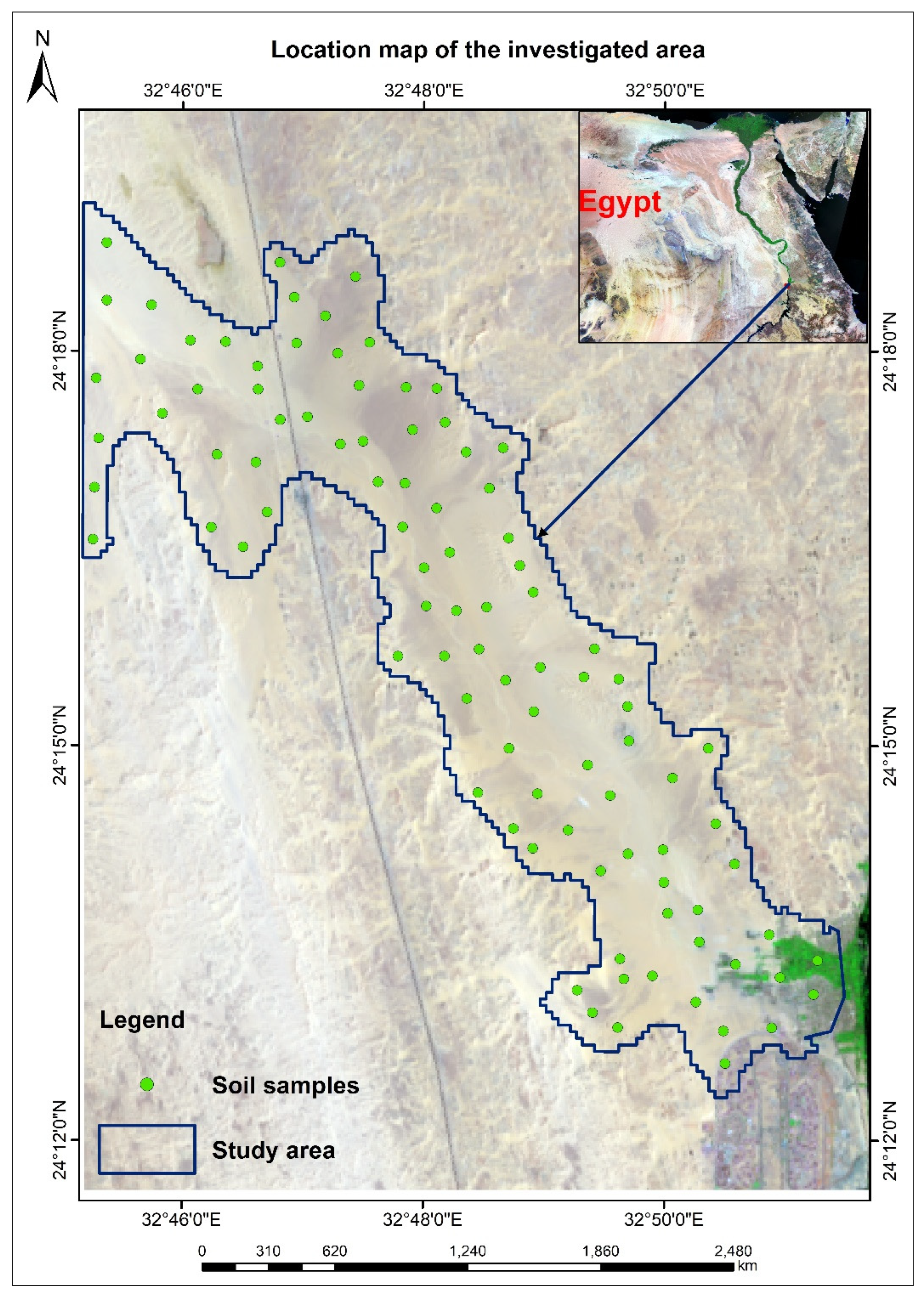
2.1. Description of the Study Area

Wadi Elkobaneyya valley is a part of the Western Desert, about 20 km from the northwest part of Aswan city. Its lies between 32°45′8.788″–32°53′00″ N and 24°12′18.546″–24°19′7.458″ E, as represented in Figure 1, and this study area covers about 42.34 km² in the Aswan Governorate, Egypt.

The study area is characterized by hot and dry summers with little rainfall in winter and bright sunshine throughout the year. Where the surface temperature is between 22.9 °C in winter and 41 °C in the summer period. The mean annual precipitation is about 0.85 mm, as shown in

Table 1. Meteorological data of the investigated area.

Climate Data for the Study Area
Month	Minimum	Maximum	Average	ST.DEV. *
Record high Tem. * °C	35.30	51.00	45.10	5.13
Average high Tem. * °C	22.90	41.40	33.62	6.75
Daily mean Tem. * °C	15.30	33.60	26.01	6.79
Average low Tem. * °C	8.70	26.00	18.48	6.28
Record low Tem. * °C	0.60	20.00	9.90	7.19
Average rainfall mm	0.00	1.40	0.22	0.43
Average rainy days (≥0.01 mm)	0.00	0.85	0.13	0.26
Average relative humidity (%)	16.00	42.00	26.17	8.79

Source: NOAA, 2022 for mean temperatures, rainfall, humidity, Meteo. Climate. Tem. *; Temperature. St. Dev. *; Standard Deviation.

. Soils in Elkobaneyya valley are generally characterized by a Hyperthermic soil temperature regime and Torric soil moisture regime, soils are mainly calcareous, and the common soil orders are Aridisols and Entisols according to the United State Department of Agriculture (USDA) soil taxonomies [52]. The elevation of the investigation area varies from 78 to 196 m Above Sea Level (ASL). The Nubian sandstones are the most important sediment rocks covering the study area. Generally, Quaternary sediments occupy most of the studied area. They were represented by Aeolian sand, sand accumulations and salt crusts [53].

2.2. Soil Sampling and Analysis

The fieldwork was conducted in February 2022, and soil samples were geo-referenced using the Global Positioning System (GPS), as shown in Figure 1. The soil samples were dug and described according to the standard scheme and terminology of the Food and Agriculture Organization (FAO, 2006) [54] and American Soil Survey Staff (2014) [52]. A total of 96 soil samples were collected and covered the recognized different soil layers in

Table 2. Soil properties descriptive statistics data.

Soil Properties
	CaCo3%	pH 1:2.5	EC (dS/cm)
Mean	1.60	7.83	0.70
Standard Deviation	1.92	0.73	0.40
Sample Variance	3.68	0.53	0.16
Minimum	0.04	5.11	0.22
Maximum	9.40	8.67	2.65
Count.	96.00

.

Soil Chemical Properties

• Total calcium carbonate (CaCO₃) was determined using Scheibler’s calcimeter [55].
• Soil reaction (pH) was measured at 25 °C using a glass electrode according to Alvarenga et al. (2012) [56].
• Soil salinity was determined as EC in soil extract using the Beckman conductivity bridge at 25 °C according to Bashour and Sayegh (2007) [57].

2.3. Processing and Analysis of Soil Spectral Data

2.3.1. Ground-Based Spectral Data Pre-Treatment

Soil spectral data collected using the ASD spectroradiometer in the laboratory conditions were arranged in text format (CSV files) for the processing stage. The obtained spectral data were in 1 nm intervals and converted to be in 5 nm intervals.

2.3.2. Models Development and Statistical Analysis

Prior to the modeling process, preliminary processing of the soil spectral readings was performed using a multiplicative scatter correction (MSC) [58] to choose an appropriate specific wavelet function and scale.

Multivariate regression models are used to model soil parameters. Many regression models are applied in soil studies, such as PLSR, ANN, MARS, ANN and RF. In the modeling part, randomly selected 70% of the soil samples were selected for calibration models for different soil properties. Rest data records (30%) were used for model validation.

Partial Least-Squares Regression (PLSR)

The PLSR is used as a developed prediction model for quantitative spectral analysis based on highly collinear predictor variables. The PLSR algorithm is running to select the orthogonal factors that increase the predictor (X spectra that are the mean-centered before decomposition) and response variables (lab data) variance. PLSR disintegrates X and y into factor scores (T) and factor loading (P and q). The remaining noise factors can be ignored. Hence residues E and f are added, as represented in the next Equations (1) and (2) [59].

X = TP+E

(1)

y = Tq+f

(2)

The calibration models and RMSE error of predictions were computed to select the optimal leave-one-out cross-validated calibration model and predict each soil parameter individually [60].

The R studio software 4.1.2 PLS package was running to develop the different soil parameters calibration and validation models using soil vis-NIR spectral data and the laboratory soil data (96 soil samples were randomly split into two groups, 70% of the data for calibration model and 30% used for setting the validation model) through the following stages [61]:

(i)

Data normalization (0 and 1 values);

(ii)

Data dividing (into two data sets; 2/3 for the calibration data set and 1/3 for the validation data);

(iii)

Data sorting (depending on their weights among the calibration and validation data sets); and

(iv)

Data outliers’ removal (remove the much higher or lower soil parameter values using a suitable method).

The Box–Cox method was used to remove outliers according to (Box and Cox 1964) [62]. The function of ‘inv-BoxCox’ was used in the (R) studio software, whereas; it applied to all calibration and validation datasets. Box–Cox transformation is a statistical technique that involves transforming the target variable (soil parameter) so that the data is subject to a normal distribution. The Box–Cox transformation helps to improve the predictive power of the calibration and validation models because it removes the noise (the outliers), Equation (3).

$$w_t=\{\begin{array}{c}\log \left(y_t\right) \mathrm{if} \lambda =0;\\ (y_t^{\lambda }-1)/\lambda \mathrm{otherwise}.\end{array}$$

(3)

where: t is the time period (not included because the data is non-time series) and λ is the parameter that was chosen; w is the transformed data of the targeted soil parameter y.

Multivariate Adaptive Regression Splines (MARS)

MARS is a non-parametric regression model introduced by Friedman (1991) [63]. It basically determines the relationship between the predictor’s dependent and set variables by fitting multiple definition linear regressions according to flexible models building [64]. The general MARS model equation is represented in the next Equation (4).

$${\mathit{y}}_{\mathit{p}}={\alpha }_0+{{\displaystyle \sum }}_{\mathit{m}=0}^{\mathit{M}}\alpha \mathit{m}\mathit{B}{\mathit{F}}_{\mathit{m}}\left(\mathit{x}\right)$$

(4)

where: $y_p$ is the predicted dependent variable;$M$ is the number of $B{F}_m$ data; ${\alpha }_0$ is the constant term; $\alpha m$ is the coefficient of single spline function; and $m$ and $B{F}_m\left(x\right)$ are the m^th truncated spline functions.

Least Square-Support Vector Regression (LS-SVR)

The LS-SVR model is used to predict the values of each soil parameter which can be used to find the best-fit line of the entire dataset; the best-fitted line of the dataset includes the maximum number of points fitted with the targeted variable (soil parameter). However, the SVR model was used in modeling the predictability of each soil parameter in this study (soil pH, soil EC and soil CaCO₃).

In the current study, an LS-SVR is used with the Gaussian Radial Basis Function (RBF) kernel as a training algorithm with polynomial kernels (Equation (6)). The RBF kernel algorithm requires two parameters for tuning, namely gamma (ɣ), which is the regularization parameter that determines the trade-off between the training error minimization and smoothness [65], and σ² which is the squared bandwidth of the Gaussian curve. For the tuning of these parameters, leave-one-out cross-validation is used for choosing the initial random parameters [66], to be optimized by means of the standard simplex method [67].

$$\mathit{K} \left({\mathit{X}}_{\mathit{i}},{\mathit{X}}_{\mathit{j}}\right)=\exp \left(-\frac{{\Vert {\mathit{X}}_{\mathit{i}}-{\mathit{X}}_{\mathit{j}}\Vert }^2}{{\sigma }^2}\right)$$

(5)

where: ɣ = 1/2 σ²; $K$ is a kernel radial basis function; $X_i$ and $X_j$ are vector points in any fixed dimensional space; and σ² is the squared bandwidth of the Gaussian curve.

The input parameters used for training the LS-SVR are the vis-NIR features that will be derived from the latent variables (LVs) calculated from the PLS regression model.

Random Forest (RF)

The RF classifier is a regression process of tree predictor’s combination of random input vector or randomly selected variables at each node on numerical values as arbitrary to class labels [68]. The RF classifier is a process to develop a training data set by randomly drawing and using the construction of individual trees for every feature; these fully developed trees are not pruned back, and one of random forest regression’s main advantages over other tree techniques [69].

The Neural Network Approach

ANN model contains the neurons minimum number of that is capable of simulating training data and feed-forward a back-propagation neural network with the Levenberg–Marquardt training algorithm has been used to find the optimal data weights [70]. Various experiments were performed using sigmoidal linear activation functions, and the over-fitting has been avoided to model development based on a number of hidden neurons selection, as shown in Figure 2. ANN equation was expressed in the following Equation (4).

$$\mathit{P}={\mathit{f}}_{\mathit{n}}\left({\mathit{b}}_0+{{\displaystyle \sum }}_{\mathit{k}=1}^{\mathit{h}}\left({\mathit{w}}_{\mathit{k}}{\mathit{f}}_{\mathit{n}}\left({\mathit{b}}_{\mathit{h}\mathit{k}}+{{\displaystyle \sum }}_{\mathit{i}=1}^{\mathit{m}}{\mathit{w}}_{\mathit{i}\mathit{k}}{\mathit{x}}_{\mathit{i}}\right)\right)\right)$$

(6)

where: $P$ is the data prediction; $f_n$ is the transfer function; $b_0$ is the output layer bias; $h$, hidden layer neurons number; $k$ is the hidden layer neuron value;$w_k$ is the connection weight between $k$ and single output neuron; $b_{hk}$ is the bias at the $k$ and $b_0$; $m$ is the number of input variables; $i$ is the layer of input; $w_{ik}$ is the connection weight between $i$ and $k$; and $x_i$ is the input value.

The data normalization process was applied to use data sets, and RMSE and RPD were calculated to quality parameters for the accuracy assessment of the ANN model.

2.3.3. Accuracy Assessment

To validate the developed prediction models, three statistical indices were used (R², RMSE and RPD) as shown in Equations (7)– (9).

The correlation coefficient (R²)

$${\mathit{R}}^2=1-\left(\frac{{{\displaystyle \sum }}_{\mathit{i}=1}^{\mathit{N}}{\left({\mathit{Y}}_{\mathit{i}}-{\hat{\mathbf{Y}}}_{\mathit{i}}\right)}^2}{{{\displaystyle \sum }}_{\mathit{i}=1}^{\mathit{N}}{\left({\mathit{Y}}_{\mathit{i}}-{\hat{\mathbf{Y}}}_{\mathit{i}}\right)}^2}\right)$$

(7)

where: $\hat{\mathrm{Y}}$ represents the values estimated by the models in the $i$th observation; $Y_i$ are the values measured or observed in the laboratory in the $i$th observation; Ȳ represents the mean of the observed values; and N is the number of observations.

Room Mean Square Error (RMSE)

$$\mathit{R}\mathit{M}\mathit{S}\mathit{E}=\sqrt{1/\mathit{n}\sum {\left(\mathit{y}-\mathit{x}\right)}_2}$$

(8)

where: y is the soil predicted values; x is the soil measured value; and n is the number of measured or predicted data values.

The Ratio of Performance Deviation (RPD)

$$\mathit{R}\mathit{P}\mathit{D}=\frac{\mathit{S}\mathit{D}}{\mathit{R}\mathit{M}\mathit{S}\mathit{E}}$$

(9)

where: SD, standard deviation.

The NIR spectra technique of different soil parameters’ predictability ability is categorized into three categories according to RPD ratio and correlation coefficient (R²) values; category (A) includes soil parameters which are highly predictable with R-square between 0.8 and 1, and with RPD above 2; category (B) includes soil parameters that can be predicted with a moderate performance of predictability whereas R-Square between 0.5 and 0.8, and the RPD is between 1.4 and 2 and category (C) that includes soil parameters which had the lowest predictability performance (R-square is lower than 0.5, and the RPD is lower than 1.4), as shown in the

Table 3. NIR spectra predictability categories of soil parameters.

NIR Category	RPD	R2	Parameters
A	<2	1−0.8	Moisture, sand, silt, exch. Ca, and CEC.
B	2−1.4	0.8−0.5	Clay, soil pH, N, K, Ca, Mg, Fe and Mn
C	>1.4	>0.5	Cu, P, Zn and Na.

[71].

2.3.4. Variables Selection Methods

For selecting the significant bands which more related to soil chemometrics, different techniques are commonly used, such as the Competitive Adaptive Reweighted Sampling (CARS) technique that was used for vis-NIR data-sets (ASD) significant bands selecting as the optimal combination of the wavelengths existing in the full spectrum using the principal of the survival of the fittest to build a high-performance calibration model based on next steps [72]:

(1)

Wavelength selection perform forced staffing;

(2)

Wavelengths competitive selection realize using Adaptive Reweighted Sampling (ARS) prediction model; and

(3)

Subset data evaluation based on cross-validation.

2.3.5. Competitive Adaptive Reweighted Sampling (CARS) Analysis

The CARS analysis was proposed to select the most relevant combination of variables (or wavelengths) during a successive selecting procedure. Based on the regression coefficients obtained by the PLS model, CARS iteratively selects N subsets of variables from N Monte Carlo (MC) sampling processes. During each process, fixed ratios of samples are randomly selected to establish a calibration model. Next, with the regression coefficients obtained, a two-step variable selection procedure is adopted to select the relevant wavelengths. Finally, cross-validation is used to choose the subset (the most relevant combination of wavelengths) showing the lowest root mean square error [73].

The method proceeds as follows:

Step 1: MC sampling:

Randomly select k samples (X_i, y_i), i stands for the ith loop. Build a PLS model based on the dominating variables Vsel_old, then record the regression coefficients beta (Equation (10)).

$$\mathit{b}\mathit{e}\mathit{t}\mathit{a}=\mathit{W}\ast \mathit{b}$$

(10)

Step 2: Sort the variables in descending order according to the absolute value of their regression coefficients. Update the ratio of variables to be kept (Equations (11), (12) and (13)).

$${\mathit{r}}_{\mathit{i}}=\mathit{a}{\mathit{e}}^{-\mathit{k}\mathit{i}}$$

(11)

$$\mathit{a}={\left(\frac{\mathit{p}}{2}\right)}^{1/\left(\mathit{N}-1\right)}$$

(12)

$$\mathit{k}=\frac{\ln \left(\mathit{p}/2\right)}{\mathit{N}-1}$$

(13)

where; ln means the natural logarithm; and N represents the number of sampling process.

The exponent function’s trace in Step 2 decreases rapidly in the first stage, whereas in the second stage, the trace progresses gently. This will facilitate the selection process [73].

Step 3: Condense the current dataset to have p×r_i variables. Then draw a subset of variables from the retained p × r_i variables using an adaptively reweighted sampling method, according to a normalized weight w_i (Equation (14)).

$${\mathit{w}}_{\mathit{i}}=\frac{\left|\mathit{b}\mathit{e}\mathit{t}{\mathit{a}}_{\mathit{i}}\right|}{{{\displaystyle \sum }}_{\mathit{i}=1}^{\mathit{p}}\left|\mathit{b}\mathit{e}\mathit{t}{\mathit{a}}_{\mathit{i}}\right|}, \mathit{i}=1, 2, 3, \dots , \mathit{p}$$

(14)

Essentially, the adaptively reweighted sampling method in Step 3 is a weighted sampling algorithm. The variables with larger weights will be selected with higher frequency, and this will accelerate the selection process.

Step 4: Compute RMSE using Vsel_new. Then Vsel_old = Vsel_new.

Step 5: Let i = i + 1. If i > N, return to step 1; else, continue.

Step 6: Choose the subset with the minimum RMSE as the optimal combination of variables/wavelengths and build the final calibration model.

2.4. Laboratory Hyperspectral Data Collection

Ninety-six ground soil samples with 2 cm thickness were scanned using Field-Spec-4 Analytical Spectral Device (ASD; Boulder, CO, USA) with wavelength ranging from 350 to 2500 nm in the laboratory condition [74]. Hyperspectral reflectance was measured under two calibrated halogen lamps (1000 W) situated at 0.70 m with a zenith angle of 30° in a dark room after sensor calibration using a white spectral panel. All recorded soil spectral signatures were converted into tab-delimited text file format using the View Spec. Pro. Software (Version 4.05) to facilitate data sharing with other software.

3. Result and Discussion

3.1. The Behavior of Soil Spectral Signatures

Figure 3 shows the spectral reflectance of soil samples; they illustrate the response and absorption areas throughout the wavelength from 1400 to 2200 nm that are associated with clay minerals, at 1400 to 1900 nm, and lattice OH (moisture adsorbed to the surface of clay) features at 1900 to 2200 nm [75].

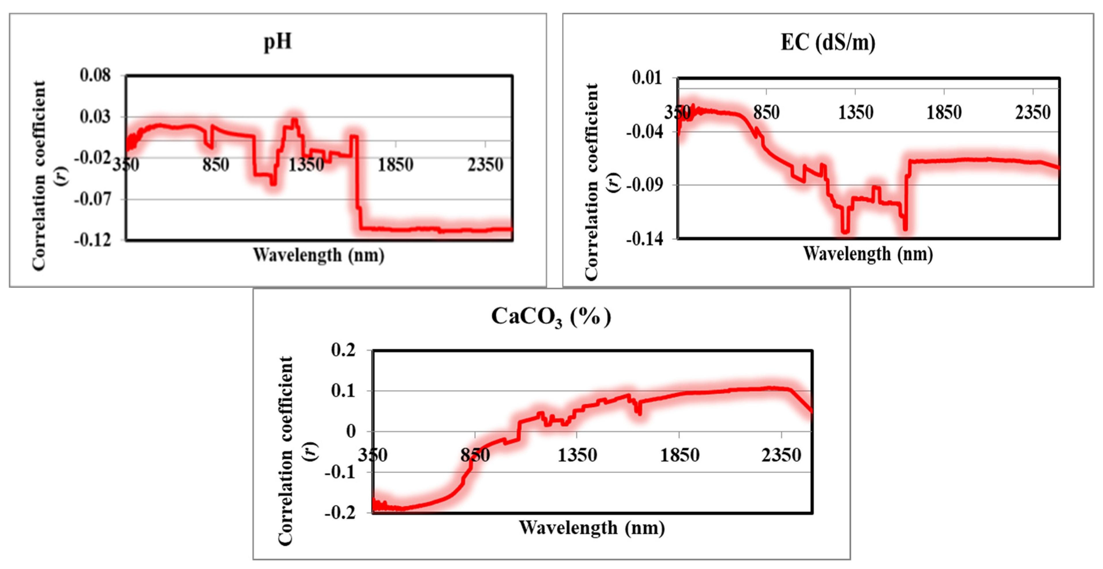
3.2. Correlation of Soil Parameters and Their Corresponding Spectral Signatures

Figure 4 and

Table 4. The most significantly correlated bands with each soil parameter.

pH
r	0.0176	0.0194	0.0271	−0.051	−0.0797	−0.105	−0.106	−0.108
Wavelengths (nm)	492	828	1276	1158	1636	1656	2068	2350
EC
r	−0.0826	−0.0985	−0.105	−0.133	−0.103	−107	−0.118	−0.131
Wavelengths (nm)	1014	1194	1222	1276	1410	1516	1602	1626
CaCO3
r	−0.185	−0.17	−0.0975	0.0459	0.0679	0.0852	0.0946	0.107
Wavelengths (nm)	470	658	812	1158	1440	1564	1860	2262

show the correlation between examined soil parameters and soil spectral signatures, the most significantly correlated bands with each soil parameter from the obtained correlation data.

The results were observed that in the pH soil parameter, the maximum correlation coefficient values were recorded as 0.0176, 0.0194, 0.0271, −0.051, −0.0797, −0.105, and −0.108 in wavelengths of 492, 828, 1276, 1158, 1636, 1656, 2068, and 2350, respectively.

The results agree with many research studies, such as Abdul Munnaf et al. (2019) [21,22,76], who found that the wavelengths 455, 772, 1361, and 1424 nm have sensitive responses for the concentration of pH. Like with the results of Mousavi et al. (2021) [77], the bands that responded to pH were 400–439, 499–566, 695–744, 874–883 and 885–914.

The result showed the most significant reflectance responses to (EC) were the following wavelengths: 1014, 1194, 1222, 1276, 1410, 1516, 1602 and 1626, and their correlation ® were: −0.0826, −0.0985, −0.105, −0.133, −0.103, −0.107, −0.106 and −0.108, respectively, this results corresponded with Mousavi et al. (2021) [77], where he showed the following bands responded to EC: 1.910–1.990, 2.102–2.103, 2.109–2.126, 2.138–2.163, 2.365–2.367. In addition, Seifi et al. (2020) [78] pointed out that the spectral reflectance data were positively correlated to soil salinity in a range of 400–1891, 2017 to 2165 and 2280–2359 nm. On the other hand, the spectral reflectance data was found to negatively correlate to soil salinity in a range of 1891–2017, 2166 to 2279 and 2360–2400 nm.

The results showed that the spectral responses of soil calcium carbonate were observed in separate places in the wavelength as follows: 470, 658, 812, 1158, 1440, 1564, 1860 and 2262, respectively, and their correlation coefficient values were −0.185, −0.170, −0.0975, 0.0459, 0.0679, 0.0852, 0.0946, and 0.107, respectively. CaCO₃ significantly influences the reflectance characteristics of soil and has spectral activity in the NIR spectral region (700–2500 nm). The strongest diagnostic vibrational absorptions are at 2300–2350 nm, and the other three weaker bands occur near 2120–2160 nm, 1997–2000 nm and 1850–1870 nm [79]. The soil spectrum characterizes complex absorption patterns with a large number of predictor variables that are highly collinear, and therefore analyses of diffuse reflectance spectra require the use of multivariate calibrations [59]. Figure 4 shows a few other prominent absorption peaks between 2200–2300 nm and around 2440 nm. According to Clark (1999) [79]. Calcium carbonate tends to increase soil brightness [80] and also exhibits diagnostic features in the infrared wavelength region, with the strongest absorption centered near 2300 nm to 2350 nm [81]. The highest values of the regression coefficients had wavelengths in the NIR spectral range of 2325 nm to 2365 nm with a peak at 2340 nm.

3.3. Estimation of Soil Parameters Using Different Models

Three multivariate regression models: PLSR, MARS and Support Vector Regression (SVR), was used for modeling the predictability of soil parameters (pH, EC and CaCO₃); based on the laboratory data (observed) and soil spectral data throughout 350 to 2500 nm.

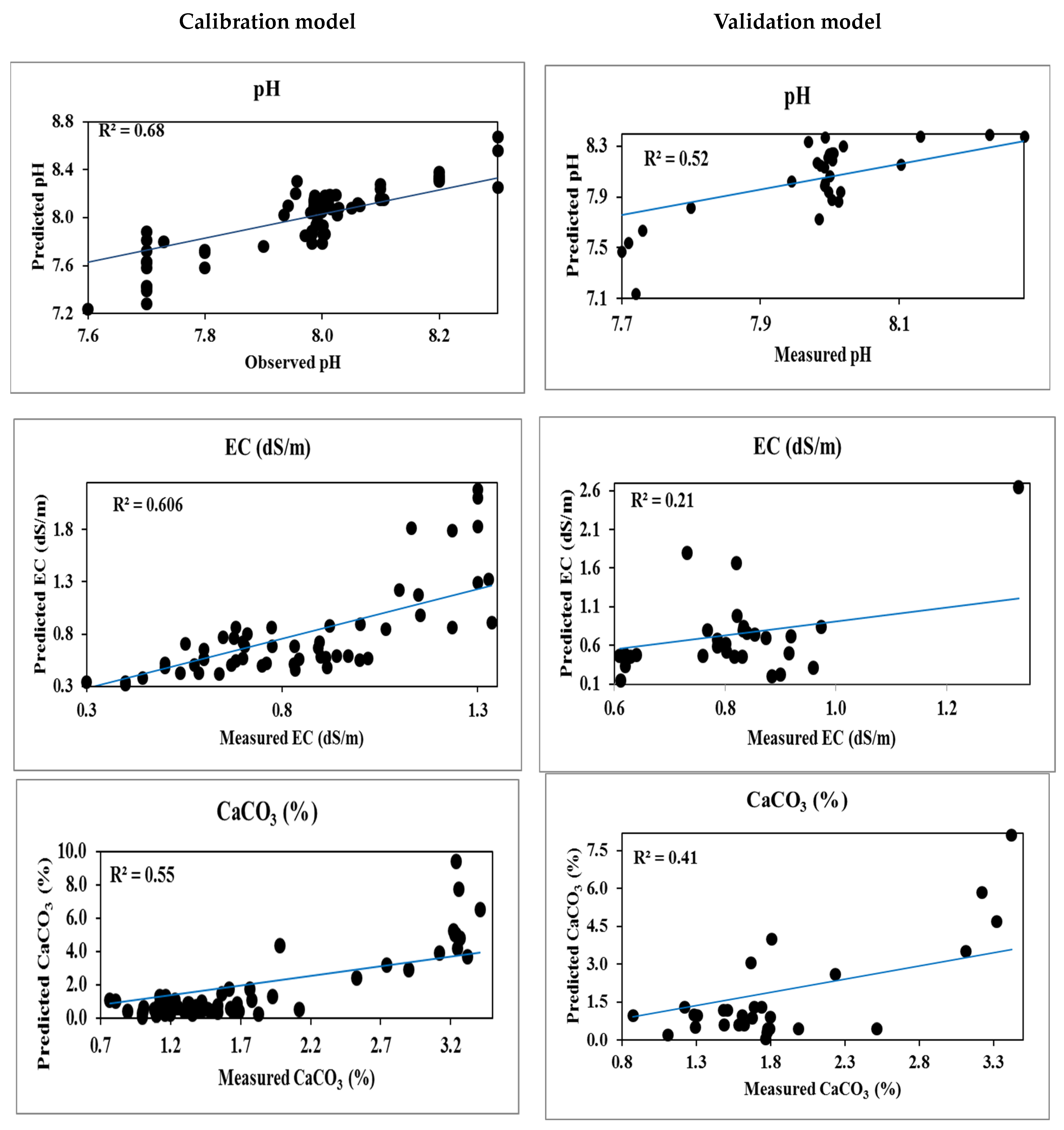
3.3.1. Partial Least Square Regression (PLSR) of Soil Parameters (pH, EC and CaCO₃)

The outliers of each calibration and validation dataset were removed, whereas the rest values were used for the modeling process. This data was divided in the internal PLSR process into ten components, whereas each component included the same number of variables.

Table 5. The predictability assessment of the soil parameters using the PLSR model.

Soil Parameter	Calibration Data-Set				Validation Data-Set
	n	RMSE	RPD	R2	n	RMSE	RPD	R2
pH	63	0.0721	2.254	0.68	26	0.0932	1.452	0.52
EC (dS/m)	65	0.0856	1.461	0.61	27	0.1112	1.316	0.21
CaCO3 (%)	66	0.0995	2.465	0.55	29	0.3519	1.881	0.41

shows the number of samples used in modeling for pH, EC and CaCO₃ after removing the outlier in calibration and validation processing. In addition, the accuracy assessment for both calibration and validation models for selected soil parameters.

Sixty-three measured pH values and their spectral data were used as data entered of the PLSR model for calibration. The RMSE value of the pH calibration model was 0.0721, while RPD and R² values were 2.254 and 0.68, respectively. The results are consistent with [21,82,83].

The predictability assessment of the pH validation model was achieved, whereas RMSE, RPD and R² values were 0.0932, 1.452 and 0.52, respectively.

The results of calibration of EC values and their corresponding spectral variables showed that the regression coefficient R² value was 0.61 while RPD and RMSE were 1.461 and 0.0856 dS/m. The results show that soil salinity can be predicted using spectral signatures, and this is consistent with the results of Zhou et al., 2022 [84]. The validation PLSR model validation of EC by RPD, RMSE and R² were 1.316, 0.1112 dS/m and 0.21, respectively.

The results of CaCO₃ calibration showed that the R² value was 0.55, RPD was 2.465, and RMSE was 0.099, these results agree with Alomar et al., 2022 [85], where the results were 0.518. 3.39 for R² and RMSE, respectively. The validation of CaCO₃ predicting was: 3519, 1.88 and 0.41 for RMSE, RPD and R², respectively, as shown in Figure 5.

For selecting the most correlated or effective bands that were chosen as inputs to derive the PLSR model component for determining the various soil parameters, the CARS technique was applied, as presented in the next Equations (15)– (17).

Soil pH parameter = 0.028 – 0.0258R₄₉₂ + 0.0628R₈₂₈ – 0.0423R₁₂₇₆ – 0.0148R₁₁₅₈ + 0.0236R₁₆₃₆ – 0.01642R₁₆₅₆ + 0.0564R_20681999 + 0.0752R₂₃₅₀

(15)

Soil EC parameter = 0.032 + 0.0364R₁₀₁₄ – 0.0569R₁₁₉₄ – 0.0547R₁₂₂₂ + 0.0258R₁₂₇₆ – 0.0364R₁₄₁₀ + 0.02145R₁₅₁₆ + 0.0675R₁₆₀₂ – 0.0827R₁₆₂₆

(16)

CaCO₃ parameter = 0.034 + 0.0358R470 – 0.0837R₆₅₈ + 0.0361R₈₁₂ + 0.0568R₁₁₅₈ + 0.0363R₁₄₄₀ – 0.02482R₁₅₆₄ + 0.0462R₁₈₆₀ – 0.0824R₂₂₆₂

(17)

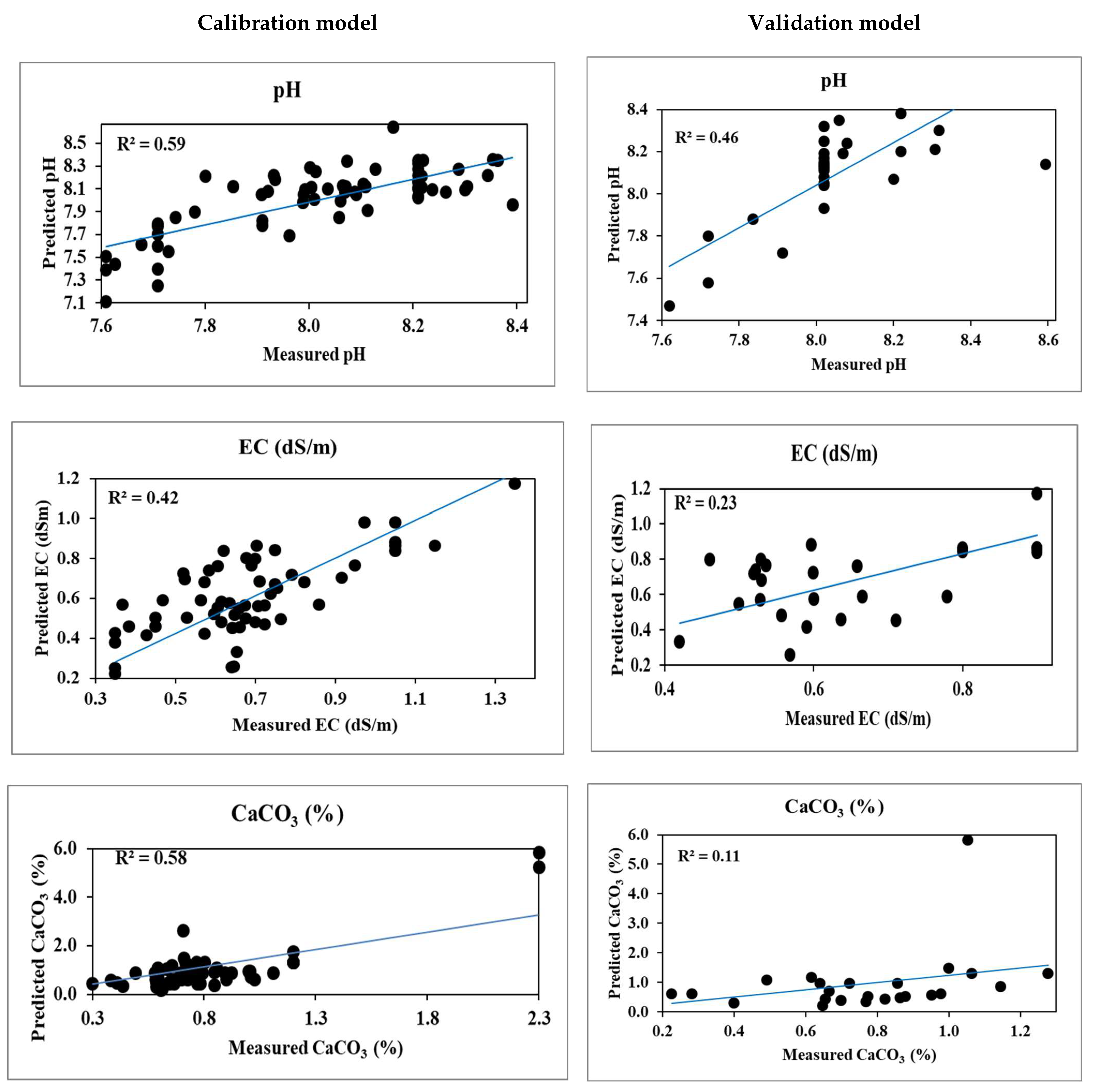
3.3.2. Multivariate Adaptive Regression Splines (MARS)

The process of removing the outliers was performed for the two datasets to enhance the predictability of each soil parameter, as well as to increase the homogeneity of the used data. However, the MARS model was developed for each soil parameter in the investigated area, and the accuracy assessment of each generated model was done and shown in

Table 6. The obtained data of MARS models for each soil parameter.

Soil Parameter	Calibration				Validation
	n	RMSE	RPD	R2	n	RMSE	RPD	R2
pH	66	0.125	1.737	0.59	29	0.136	1.413	0.46
EC (dS/m)	67	0.139	1.491	0.42	29	0.153	0.957	0.23
CaCO3 (%)	67	0.256	1.421	0.58	29	0.289	0.898	0.11

.

The obtained data of the MARS models for each soil parameter are explained as follows.

The MARS calibration model performance of the soil pH parameter was tested, whereas the R² value was 0.59, RMSE was 0.125, and RPD was 1.737. No soil pH values were removed from the validation dataset. The RMSE, RPD, and R² values for the soil pH validation model were 0.136, 1.413 and 0.46, respectively.

The calibration result estimation of the soil EC was an R² value of 0.42, while the RPD and RMSE values were 1.491 and 0.139 dS/m, respectively. Moreover, for the MARS validation model, R², RPD and RMSE were calculated, and their values were 0.23, 0.975, and 0.153 dS/m, respectively.

Furthermore, the results showed that an R² value of 0.58 was recorded for estimating the soil content of CaCO₃, while the R² value was 0.11 for the validation model. The RMSE value was 0.256 for calibration and validation 0.289 for validation models. The RPD value of the calibration model was 1.421, while 0.898% for the validation, as shown in Figure 6.

The MARS model deals with data as subsets or pieces to detect dependent variables (soil parameter) and a set of predictors (spectral variables) relationships using individual linear regressions with two or more spline functions. These results agree with the results of [86,87], for pH and EC.

3.3.3. Support Vector Regression (SVR) Model

The SVR was used for modeling the soil (pH, EC and CaCO₃), the outliers were removed, while 65 soil pH values were used for calibration. The results showed that R², RMSE and RPD values were 0.66, 0.0977 and 1.844, respectively. The SVR validation model (n = 28) was able to estimate the soil pH parameter by which R² = 0.41, RPD = 1.420 and RMSE = 0.113.

To calibrate the SVR model using 66 values of soil EC was conducted. The obtained results of the SVR calibration model showed that R² of regression was 0.70, while RPD was 1.330, and RMSE was 0.3961 dS/m. In the SVR validation model, lower performance was recorded (R² = 0.26, RPD = 0.555, and RMSE = 0.369 dS/m) for predicting the soil EC parameter.

Two CaCO₃ outliers were removed, and the rest data were used for calibration and validation. The R², RPD and RMSE in the SVR calibration model were 0.74, 1.784, and 0.7953%, respectively, while the validation results in the SVR model were (R² = 0.47, RPD = 1.247, and RMSE = 0.666%). The obtained results showed that the SVR has the advantage compared with PLSR and MARS for predicting pH, EC and CaCO₃. Their other studies support our results, such as [88,89].

The randomization process for selecting the entire data in each dataset is very important in SVR modeling of soil parameters to ensure the un-bias of the obtained outputs of both calibration and validation processes. Mouazen et al. (2010) [90] adopted a similar approach, where the latent variables obtained from PLSR were used as input to a Back Propagation Artificial Neural Network (BPNN), not to SVR as done in the current work.

As PLSR and MARS models, SVR was assessed for its performance in predicting and estimating soil pH, EC and CaCO₃ and the values of the evaluation parameters were presented in

Table 7. The obtained data of SVR models for each soil parameter.

Soil Parameter	Calibration				Validation
	n	RMSE	RPD	R2	n	RMSE	RPD	R2
pH	65	0.0977	1.844	0.66	28	0.113	1.420	0.41
EC (dS/m)	66	0.3961	1.330	0.70	29	0.369	0.555	0.26
CaCO3 (%)	66	0.7953	1.784	0.74	29	0.666	1.247	0.47

.

The observed and predicted soil parameters data scatter plot based on SVR calibration and validation models are shown in Figure 7.

3.4. The Machine Learning Models for Predicting Soil Parameters

The RF and ANN machine learning algorithms were used in this study to associate a large number of inputs and resulting outputs set with higher predictability through three steps of training, testing and validating and predicting the various soil parameters (pH, EC and CaCO₃). However, the RF and ANN outputs are discussed in the following parts.

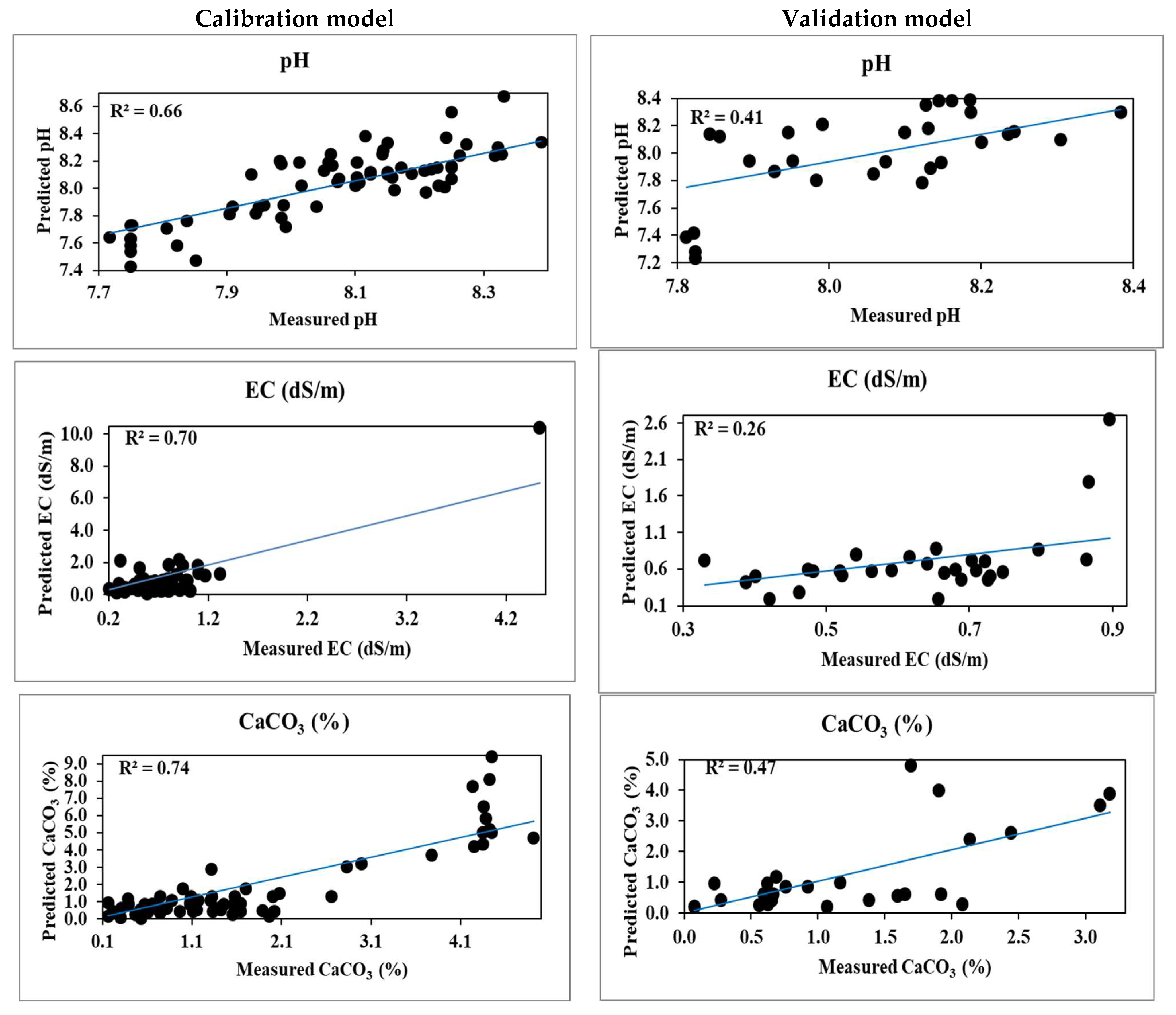
3.4.1. Random Forest (RF)

By the bragging process, training data is developed through a combination of randomly selected variables at each node to mature a tree. The same process occurs in the following steps of testing and validation. The obtained data of the RF model of calibration and validation are demonstrated in

Table 8. The obtained data of RF models for each soil parameter.

Soil Parameter	Calibration				Validation
	n	RMSE	RPD	R2	n	RMSE	RPD	R2
pH	65	0.0572	2.975	0.82	28	0.0686	2.339	0.57
EC (dS/m)	66	0.15800	2.231	0.78	29	0.1082	2.343	0.81
CaCO3 (%)	67	0.3568	3.268	0.83	29	0.2978	2.659	0.75

.

Figure 8 showed the fitting of each RF calibration and validation model, whereas the observed pH values were plotted and the estimated pH values. As calibration and validation accuracy parameters, R², RPD and RMSE were calculated, R² = 0.82 for calibration and 0.57 for validation. The RPD of the calibration was 2.975, and the RPD of the validation was 2.339. The RMSE values of the RF calibration and validation models were 0.0572 and 0.0686, respectively.

The obtained results of modeling EC using the RF calibration model showed that RMSE, RPD and R² were 0.1580, 2.231 and 0.78, respectively. Meanwhile, the validation models were 0.1082, 2.343 and 0.81 for RMSE RPD and R², respectively. This result was matched with [91,92].

The obtained results of modeling CaCO₃ using the RF calibration model showed that RMSE, RPD and R² were 0.3568, 3.268 and 0.83, respectively. Meanwhile, hand the validation models were 0.2978, 2.659 and 0.75 for RMSE, RPD and R², respectively. The RF scatter plots, calibration, and validation models are presented in Figure 8.

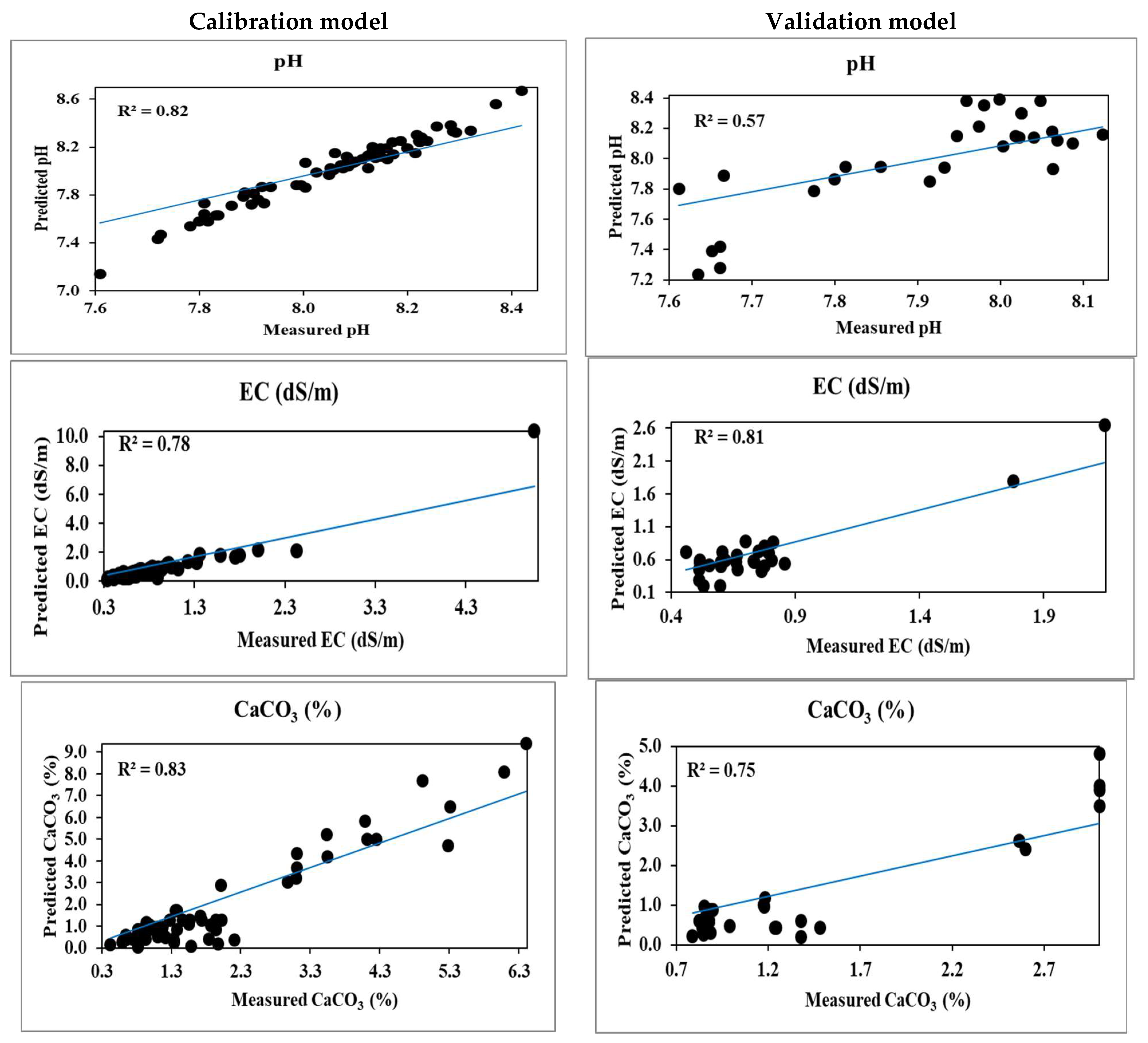
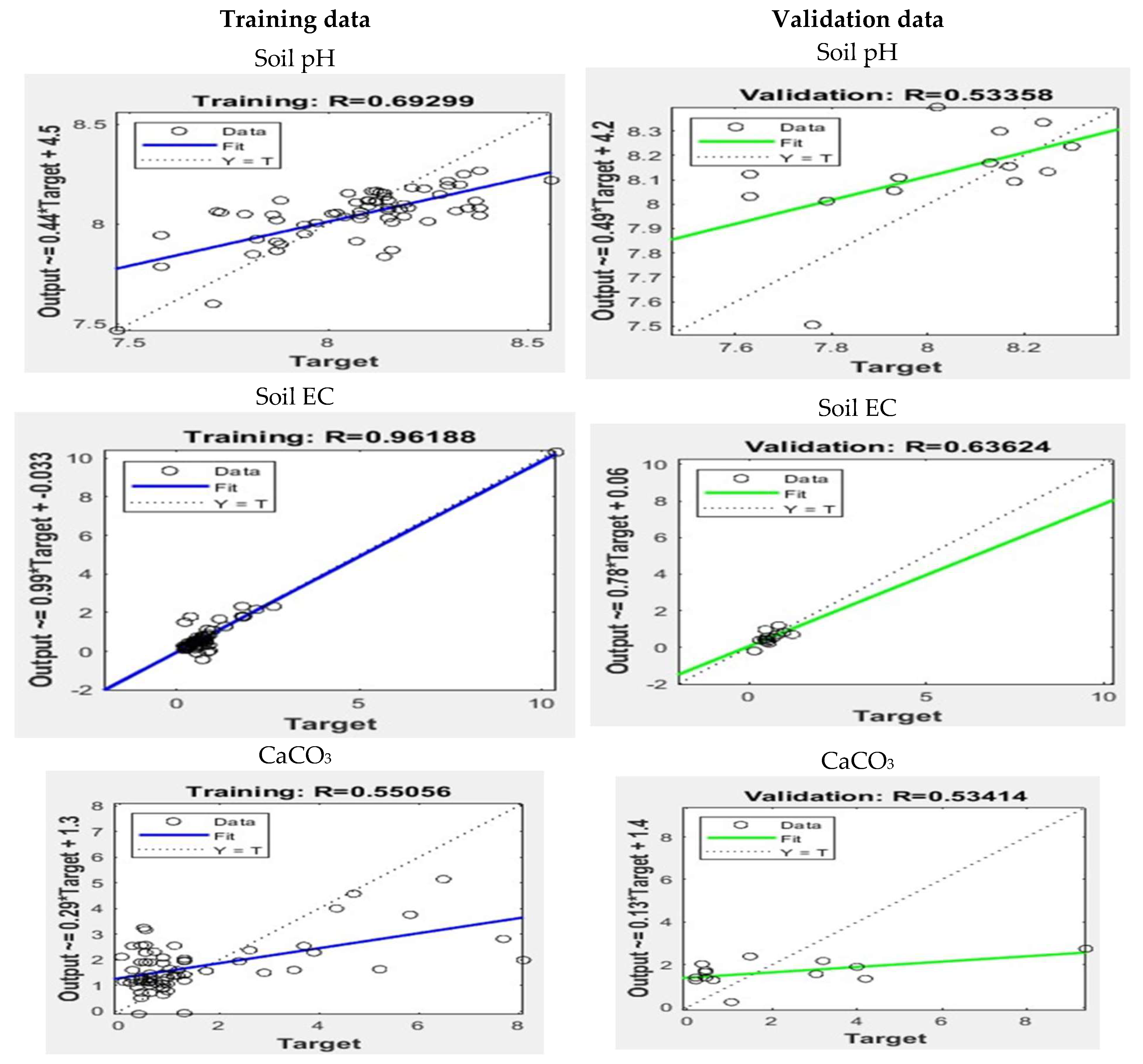
3.4.2. Artificial Neural Network (ANN)

The ANN consists of input, hidden and output layers with connected neurons (nodes) to estimate the unknown inputs. The inputs are the soil combined with observed data from the laboratory and spectra. An ANN model was performed to predict soil pH, EC and CaCO₃ and its outputs are presented in

Table 9. The obtained data of ANN models for each soil parameter.

Soil Parameter	Calibration				Validation
	n	RMSE	RPD	R2	n	RMSE	RPD	R2
pH	65	0.2391	1.438	0.69	15	0.2592	1.385	0.53
EC (dS/m)	66	0.4866	2.248	0.96	15	0.5016	1.869	0.64
CaCO3 (%)	65	1.670	1.149	0.55	14	1.723	1.114	0.53

.

The training model of ANN was tested for its accuracy, whereas RMSE was 0.2391, RPD was 1.438, and R² was 0.69 for soil pH. Regarding the ANN validation model, R² = 0.53, RMSE = 0.2592, and RPD = 1.385.

Figure 9 shows the scatter plotting of observed EC values and predicted EC values for training and validating steps using the ANN model.

The Calibration model of EC showed high performance as R² was 0.96, RMSE was 0.486, and RPD was 2.248.

The ANN validation model showed that R², RPD and RMSE values were 0.64, 1.869, and 0.5016 dS/m, respectively.

The predictability of the soil CaCO₃ was evaluated, with R² as 0.55 in the ANN training step, while it was 0.53 in the validation step. The RPD values in the ANN training and validation were 1.149 and 1.114, respectively, while the RMSE values for the two ANN models were 1.670 and 1.723%.

The relationship between measured and predicted soil parameters was demonstrated in Figure 9 for training and validation ANN models, respectively.

4. Conclusions

The current study aims to characterize and develop prediction models and evaluate the accuracy and predictability of Soil EC, pH and CaCO₃ in some soils using vis-NIR spectroscopy data in arid lands (the Elkobaneyya valley). Three multivariate regression models, PLSR, MARS, and SVR and two machine learning models were used. The PLSR model is the best model for predicting soil pH in terms of calibration and validation, where R² = 0.68 and 0.52, and the SVR model was the best model for predicting soil EC and CaCO_3, where they were R² 0.70 and 0.74, respectively for calibration. Meanwhile, the R² values were 0.26 and 0.47 for validation. The RF and ANN have good results in predicting these parameters. The result showed that the best model to predict soil pH and CaCO₃ is RF, where R² values were 0.82 and 0.83 for calibration, and 0.57 and 0.75 for validation, respectively. Furthermore, the best model for predicting soil EC was ANN; the R² was 0.96 for calibration and 0.8 for validation for selecting the most correlated bands or effective for predicting the various soil parameters. CARS technique was applied to disengage the high-response bands to soil pH; the significant bands were 492, 828, 1276, 1158, 1636, 1656, 2068, and 2350. Whereas for soil EC parameters, the significant bands were 1014, 1194, 1222, 1276, 1410, 1516, 1602 and 1626. Additionally, regarding the soil CaCO₃, the significant bands were 470, 658, 812, 1158, 1440, 1564, 1860 and 2262.

The final results showed that RF has advantages over ANN in predicting the PH and CaCO₃ in calibration and validation. Additionally, ANN has the advantage of predicting the EC more than RF.

References

1. Gunina, A.; Kuzyakov, Y. From energy to (soil organic) matter. Glob. Change Biol. 2022, 28, 2169–2182. [Google Scholar] [CrossRef]
2. El Behairy, R.A.; El Baroudy, A.A.; Ibrahim, M.M.; Mohamed, E.S.; Kucher, D.E.; Shokr, M.S. Assessment of Soil Capability and Crop Suitability Using Integrated Multivariate and GIS Approaches toward Agricultural Sustainability. Land 2022, 11, 1027. [Google Scholar] [CrossRef]
3. Abdel-Fattah, M.K.; Mohamed, E.S.; Wagdi, E.M.; Shahin, S.A.; Aldosari, A.A.; Lasaponara, R.; Alnaimy, M.A. Quantitative evaluation of soil quality using Principal Component Analysis: The case study of El-Fayoum depression Egypt Sustainability. Land 2021, 13, 1824. [Google Scholar] [CrossRef]
4. Abu-hashim, M.; Lilienthal, H.; Schnug, E.; Kucher, D.E.; Mohamed, E.S. Tempo-Spatial Variations in Soil Hydraulic Properties under Long-Term Organic Farming. Land 2022, 11, 1655. [Google Scholar] [CrossRef]
5. Nocita, M.; Stevens, A.; van Wesemael, B.; Aitkenhead, M.; Bachmann, M.; Barthès, B.; Wetterlind, J. Soil spectroscopy: An alternative to wet chemistry for soil monitoring. Adv. Agron. 2015, 132, 139–159. [Google Scholar]
6. Abuzaid, A.S.; Abdellatif, A.D.; Fadl, M.E. Modeling soil quality in Dakahlia Governorate, Egypt using GIS techniques. Egypt. J. Remote Sens. Space Sci. 2021, 24, 255–264. [Google Scholar] [CrossRef]
7. Rossel, R.V.; Walvoort, D.J.J.; McBratney, A.B.; Janik, L.J.; Skjemstad, J.O. Visible, near infrared, mid infrared or combined diffuse reflectance spectroscopy for simultaneous assessment of various soil properties. Geoderma 2006, 131, 59–75. [Google Scholar] [CrossRef]
8. Sarathjith, M.; Bhabani, S.D.; Suhas, P.W.; Kanwar, L.S.; Abhinav, G. Comparison of data mining approaches for estimating soil nutrient contents using diffuse reflectance spectroscopy. Curr. Sci. 2016, 110, 1031–1037. [Google Scholar] [CrossRef]
9. Sayed, Y.A.; Fadl, M.E. Agricultural sustainability evaluation of the new reclaimed soils at Dairut Area, Assiut, Egypt using GIS modeling. Egypt. J. Remote Sens. Space Sci. 2021, 24, 707–719. [Google Scholar] [CrossRef]
10. Hicks, W.; Rossel, R.V.; Tuomi, S. Developing the Australian mid-infrared spectroscopic database using data from the Australian Soil Resource Information System. Soil Res. 2015, 53, 922–931. [Google Scholar] [CrossRef]
11. Singh, S. Remote sensing applications in soil survey and mapping: A Review. Int. J. Geomat. Geosci. 2016, 7, 192–203. [Google Scholar]
12. Wollenhaupt, N.; Wolkowski, R.; Clayton, M. Mapping soil test phosphorus and potassium for variable-rate fertilizer application. J. Prod. Agric. 1994, 7, 441–448. [Google Scholar] [CrossRef]
13. Ji, W.; Adamchuk, V.I.; Biswas, A.; Dhawale, N.M.; Sudarsan, B.; Zhang, Y.; Shi, Z. Assessment of soil properties in situ using a prototype portable MIR spectrometer in two agricultural fields. Biosyst. Eng. 2016, 152, 14–27. [Google Scholar] [CrossRef]
14. Selmy, S.A.; Al-Aziz, S.H.A.; Jiménez-Ballesta, R.; García-Navarro, F.J.; Fadl, M.E. Soil Quality Assessment Using Multivariate Approaches: A Case Study of the Dakhla Oasis Arid Lands. Land 2021, 10, 1074. [Google Scholar] [CrossRef]
15. Demattê, J.A.; Alves, M.R.; Gallo, B.C.; Fongaro, C.T.; Souza, A.B.; Romero, D.J.; Sato, M.V. Hyperspectral remote sensing as an alternative to estimate soil attributes. Rev. Ciência Agronômica 2015, 46, 223–232. [Google Scholar] [CrossRef]
16. Soriano-Disla, J.M.; Janik, L.J.; Viscarra Rossel, R.A.; Macdonald, L.M.; McLaughlin, M.J. The performance of visible, near-, and mid-infrared reflectance spectroscopy for prediction of soil physical, chemical, and biological properties. Appl. Spectrosc. Rev. 2014, 49, 139–186. [Google Scholar] [CrossRef]
17. Abuzaid, A.S.; AbdelRahman, M.A.; Fadl, M.E.; Scopa, A. Land degradation vulnerability mapping in a newly-reclaimed desert oasis in a hyper-arid agro-ecosystem using AHP and geospatial techniques. Agronomy 2021, 11, 1426. [Google Scholar] [CrossRef]
18. Selmy, S.A.; Al-Aziz, S.H.A.; Jiménez-Ballesta, R.; García-Navarro, F.J.; Fadl, M.E. Modeling and Assessing Potential Soil Erosion Hazards Using USLE and Wind Erosion Models in Integration with GIS Techniques: Dakhla Oasis, Egypt. Agriculture 2021, 11, 1124. [Google Scholar] [CrossRef]
19. Fadl, M.E.; Abuzaid, A.S.; AbdelRahman, M.A.; Biswas, A. Evaluation of desertification severity in El-Farafra Oasis, Western Desert of Egypt: Application of modified MEDALUS approach using wind erosion index and factor analysis. Land 2021, 11, 54. [Google Scholar] [CrossRef]
20. Mohamed, E.; Ali, A.M.; El Shirbeny, M.A.; Abd El Razek, A.A.; Savin, I.Y. Near infrared spectroscopy techniques for soil contamination assessment in the Nile Delta. Eurasian Soil Sci. 2016, 49, 632–639. [Google Scholar] [CrossRef]
21. Mohamed, E.S.; Baroudy, A.A.E.; El-Beshbeshy, T.; Emam, M.; Belal, A.A.; Elfadaly, A.; Lasaponara, R. Vis-nir spectroscopy and satellite landsat-8 oli data to map soil nutrients in arid conditions: A case study of the northwest coast of egypt. Remote Sens. 2020, 12, 3716. [Google Scholar] [CrossRef]
22. Hammam, A.A.; Mohamed, W.S.; Sayed, S.E.E.; Kucher, D.E.; Mohamed, E.S. Assessment of Soil Contamination Using GIS and Multi-Variate Analysis: A Case Study in El-Minia Governorate, Egypt. Agronomy 2022, 12, 1197. [Google Scholar] [CrossRef]
23. Bartholomeus, H.; Kooistra, L.; Stevens, A.; van Leeuwen, M.; van Wesemael, B.; Ben-Dor, E.; Tychon, B. Soil organic carbon mapping of partially vegetated agricultural fields with imaging spectroscopy. Int. J. Appl. Earth Obs. Geoinf. 2011, 13, 81–88. [Google Scholar] [CrossRef]
24. Stevens, A.; van Wesemael, B.; Bartholomeus, H.; Rosillon, D.; Tychon, B.; Ben-Dor, E. Laboratory, field and airborne spectroscopy for monitoring organic carbon content in agricultural soils. Geoderma 2008, 144, 395–404. [Google Scholar] [CrossRef] [Green Version]
25. Mohamed, E.S.; Saleh, A.M.; Belal, A.B.; Gad, A. Application of near-infrared reflectance for quantitative assessment of soil properties. Egypt J. Remote Sens. Space Sci. 2018, 21, 1–14. [Google Scholar] [CrossRef]
26. Ogen, Y.; Zaluda, J.; Francos, N.; Goldshleger, N.; Ben-Dor, E. Cluster-based spectral models for a robust assessment of soil properties. Geoderma 2019, 340, 175–184. [Google Scholar] [CrossRef]
27. Chabrillat, S.; Ben-Dor, E.; Viscarra Rossel, R. Quantitative soil spectroscopy. Appl. Environ. Soil Sci. 2013, 2013, 1–3. [Google Scholar] [CrossRef] [Green Version]
28. Dor, E.B.; Ong, C.; Lau, I.C. Reflectance measurements of soils in the laboratory: Standards and protocols. Geoderma 2015, 245, 112–124. [Google Scholar]
29. Lagacherie, P.; Baret, F.; Feret, J.B.; Netto, J.M.; Robbez-Masson, J.M. Estimation of soil clay and calcium carbonate using laboratory, field and airborne hyperspectral measurements. Remote Sens. Environ. 2008, 112, 825–835. [Google Scholar] [CrossRef]
30. AbdelRahman, M.A.; Natarajan, A.; Srinivasamurthy, C.A.; Hegde, R. Estimating soil fertility status in physically degraded land using GIS and remote sensing techniques in Chamarajanagar district, Karnataka, India. Egypt J. Remote Sens. Space Sci. 2016, 19, 95–108. [Google Scholar] [CrossRef] [Green Version]
31. AbdelRahman, M.A.; Tahoun, S. GIS model-builder based on comprehensive geostatistical approach to assess soil quality. Remote Sens. Appl. Soc. Environ. 2019, 13, 204–214. [Google Scholar] [CrossRef]
32. O’rourke, S.; Holden, N. Optical sensing and chemometric analysis of soil organic carbon—A cost effective alternative to conventional laboratory methods? Soil Use Manag. 2011, 27, 143–155. [Google Scholar] [CrossRef]
33. Santra, P.; Sahoo, R.N.; Das, B.S.; Samal, R.N.; Pattanaik, A.K.; Gupta, V.K. Estimation of soil hydraulic properties using proximal spectral reflectance in visible, near-infrared, and shortwave-infrared (VIS–NIR–SWIR) region. Geoderma 2009, 152, 338–349. [Google Scholar] [CrossRef]
34. Stenberg, B. Effects of soil sample pretreatments and standardised rewetting as interacted with sand classes on Vis-NIR predictions of clay and soil organic carbon. Geoderma 2010, 158, 15–22. [Google Scholar] [CrossRef] [Green Version]
35. Kadupitiya, H.K.; Sahoo, R.N.; Ray, S.S.; Chopra, U.K.; Chakraborty, D.; Nayan, A. Quantitative assessment of soil chemical properties using visible (VIS) and near-infrared (NIR) proximal hyperspectral data. Trop. Agric. 2010, 158, 41–60. [Google Scholar]
36. Margate, D.E.; Shrestha, D.P. The use of hyperspectral data in identifying ‘desert-like’soil surface features in Tabernas area, southeast Spain. In Proceedings of the 22nd Asian Conference on Remote Sensing, Singapore, 5–9 November 2001. [Google Scholar]
37. Wold, S.; Sjöström, M.; Eriksson, L. PLS-regression: A basic tool of chemometrics. Chemom. Intell. Lab. Syst. 2001, 58, 109–130. [Google Scholar] [CrossRef]
38. Muñoz, J.; Felicísimo, Á.M. Comparison of statistical methods commonly used in predictive modelling. J. Veg. Sci. 2004, 15, 285–292. [Google Scholar] [CrossRef]
39. Díaz-Uriarte, R.; Alvarez de Andrés, S. Gene selection and classification of microarray data using random forest. BMC Bioinform. 2006, 7, 1–13. [Google Scholar] [CrossRef] [Green Version]
40. Woodcock, C.E. Uncertainty in Remote Sensing; Wiley: Hoboken, NJ, USA, 2002; pp. 19–24. [Google Scholar]
41. Gore, R.D.; Nimbhore, S.S.; Gawali, B.W. Understanding Soil Spectral Signature though RS and GIS Techniques. Int. J. Eng. Res. Gen. Sci. 2015, 3. [Google Scholar]
42. Lausch, A.; Zacharias, S.; Dierke, C.; Pause, M.; Kühn, I.; Doktor, D.; Werban, U. Analysis of vegetation and soil patterns using hyperspectral remote sensing, EMI, and gamma-ray measurements. Vadose Zone J. 2013, 12, 1–15. [Google Scholar] [CrossRef]
43. Mustard, J.F.; Sunshine, J.M. Spectral analysis for earth science: Investigations using remote sensing data. Remote Sens. Earth Sci. Man. Remote Sens. 1999, 3, 251–307. [Google Scholar]
44. Brown, D.J.; Shepherd, K.D.; Walsh, M.G.; Mays, M.D.; Reinsch, T.G. Global soil characterization with VNIR diffuse reflectance spectroscopy. Geoderma 2006, 132, 273–290. [Google Scholar] [CrossRef]
45. Ashokkumar, H.; Prasad, J. Some typical sugarcane-growing soils of Ahmadnagar district of Maharashtra: Their characterization and classification and nutritional status of soils and plants. J. Indian Soc. Soil Sci. 2010, 58, 257–266. [Google Scholar]
46. Stenberg, B.; Rossel, R.A.V.; Mouazen, A.M.; Wetterlind, J. Visible and near infrared spectroscopy in soil science. Adv. Agron. 2010, 107, 163–215. [Google Scholar]
47. Vapnik, V. The Nature of Statistical Learning Theory; Springer Science & Business Media: Berlin/Heidelberg, Germany, 1999. [Google Scholar]
48. Vapnik, V.N.; Vapnik, V. Statistical Learning Theory; Wiley: New York, NY, USA, 1998; Volume 1. [Google Scholar]
49. Garfagnoli, F.; Ciampalini, A.; Moretti, S.; Chiarantini, L.; Vettori, S. Quantitative mapping of clay minerals using airborne imaging spectroscopy: New data on Mugello (Italy) from SIM-GA prototypal sensor. Eur. J. Remote Sens. 2013, 46, 1–17. [Google Scholar] [CrossRef] [Green Version]
50. Jain, R.; Kumar, A.; Sharma, R.U. Study of Mineral Mapping Techniques Using Airborne Hyperspectral Data: Exploring the Potential of AVIRIS-NG for Mineral Identification; Lap Lambert Academic Publishing: Saarland, Germany, 2018. [Google Scholar]
51. Ge, Y.; Thomasson, J.A.; Sui, R. Remote sensing of soil properties in precision agriculture: A review. Front. Earth Sci. 2011, 5, 229–238. [Google Scholar] [CrossRef]
52. Staff, S.S. Keys to Soil Taxonomy; United States Department of Agriculture: Washington, DC, USA, 2014.
53. Embabi, N.S. The karstified carbonate platforms in the Western Desert. In Landscapes and Landforms of Egypt; World Geomorphological Landscapes; Springer: Cham, Switzerland, 2018; pp. 85–104. ISBN 978-3-319-65659-5. [Google Scholar] [CrossRef]
54. Jahn, R.; Blume, H.P.; Asio, V.B.; Spaargaren, O.; Schad, P. Guidelines for Soil Description; FAO: Rome, Italy, 2006; ISBN 9789251055212-97. [Google Scholar]
55. Nelson, R. Carbonate and gypsum. In Methods of Soil Analysis: Part 2; Chemical and Microbiological; Wiley: Medison, WI, USA, 1982; pp. 181–198. [Google Scholar]
56. Alvarenga, P.; Palma, P.; De Varennes, A.; Cunha-Queda, A.C. A contribution towards the risk assessment of soils from the São Domingos Mine (Portugal): Chemical, microbial and ecotoxicological indicators. Environ. Pollut. 2012, 161, 50–56. [Google Scholar] [CrossRef] [PubMed]
57. Bashour, I.I.; Sayegh, A.H. Methods of Analysis for Soils of Arid and Semi-Arid Regions; FAO: Rome, Italy, 2007. [Google Scholar]
58. Liu, W.; Frédéric, B.; Gu, X.; Tong, Q.; Zheng, L.; Zhang, B. Relating soil surface moisture to reflectance. Remote Sens. Environ. 2002, 81, 238–246. [Google Scholar]
59. Rinnan, Å.; Van Den Berg, F.; Engelsen, S.B. Review of the most common pre-processing techniques for near-infrared spectra. TrAC Trends Anal. Chem. 2009, 28, 1201–1222. [Google Scholar] [CrossRef]
60. Martens, H.; Naes, T. Multivariate Calibration; John Willey & Sons. Inc.: New York, NY, USA, 1989. [Google Scholar]
61. Efron, B.; Tibshirani, R.J. An Introduction to the Bootstrap; Monographs on Statistics and Applied Probability: New York, NY, USA, 1994; Volume 57, pp. 10001–12299. [Google Scholar]
62. van der Voet, H. Comparing the predictive accuracy of models using a simple randomization test. Chemom. Intell. Lab. Syst. 1994, 25, 313–323. [Google Scholar] [CrossRef]
63. Box, G.E.; Cox, D.R. An analysis of transformations. J. R. Stat. Soc. Ser. B 1964, 26, 211–243. [Google Scholar] [CrossRef]
64. Friedman, J.H. Multivariate adaptive regression splines. Ann. Stat. 1991, 19, 1–67. [Google Scholar] [CrossRef]
65. Acciani, C.; Fucilli, V.; Sardaro, R. Data mining in real estate appraisal: A model tree and multivariate adaptive regression spline approach. In Data Mining in Real Estate Appraisal: A Model Tree and Multivariate Adaptive Regression Spline Approach; Firenze University Press: Florence, Italy, 2011; pp. 27–45. [Google Scholar]
66. De Brabanter, K.; Karsmakers, P.; Ojeda, F.; Alzate, C.; De Brabanter, J.; Pelckmans, K.; Suykens, J.A.K. LS-SVMlab Toolbox User’s Guide; Version 1.8; Katholieke Universiteit Leuven, Department of Electrical Engineering: Leuven-Heverlee, Belgium, 2011. [Google Scholar]
67. Stone, M. Cross-validatory choice and assessment of statistical predictions. J. R. Stat. Soc. Ser. B 1974, 36, 111–133. [Google Scholar] [CrossRef]
68. Pelckmans, K.; Suykens, J.A.; Van Gestel, T.; De Brabanter, J.; Lukas, L.; Hamers, B.; Vandewalle, J. LS-SVMlab: A Matlab/c Toolbox for Least Squares Support Vector Machines; Tutorial. KULeuven-ESAT: Leuven, Belgium, 2002; Volume 142. [Google Scholar]
69. Breiman, L. Random forests. Mach. Learn. 2001, 45, 5–32. [Google Scholar] [CrossRef] [Green Version]
70. Quinlan, J.R. Combining instance-based and model-based learning. In Proceedings of the Tenth International Conference on Machine Learning, Amherst, MA, USA, 27–29 July 1993. [Google Scholar]
71. Boger, Z.; Guterman, H. Knowledge extraction from artificial neural network models. In Proceedings of the 1997 IEEE International Conference on Systems, Man, and Cybernetics, Computational Cybernetics and Simulation, Orlando, FL, USA, 12–15 October 1997. [Google Scholar]
72. Chang, C.W.; Laird, D.A.; Mausbach, M.J.; Hurburgh, C.R. Near-infrared reflectance spectroscopy–principal components regression analyses of soil properties. Soil Sci. Soc. Am. J. 2001, 65, 480–490. [Google Scholar] [CrossRef] [Green Version]
73. Li, S.; Ji, W.; Chen, S.; Peng, J.; Zhou, Y.; Shi, Z. Potential of VIS-NIR-SWIR spectroscopy from the Chinese Soil Spectral Library for assessment of nitrogen fertilization rates in the paddy-rice region, China. Remote Sens. 2015, 7, 7029–7043. [Google Scholar] [CrossRef] [Green Version]
74. Li, H.; Liang, Y.; Xu, Q.; Cao, D. Key wavelengths screening using competitive adaptive reweighted sampling method for multivariate calibration. Anal. Chim. Acta 2009, 648, 77–84. [Google Scholar] [CrossRef]
75. Shepherd, K.D.; Walsh, M.G. Infrared spectroscopy—Enabling an evidence-based diagnostic surveillance approach to agricultural and environmental management in developing countries. J. Near Infrared Spectrosc. 2007, 15, 1–19. [Google Scholar] [CrossRef]
76. Abdul Munnaf, M.; Nawar, S.; Mouazen, A.M. Estimation of secondary soil properties by fusion of laboratory and on-line measured Vis–NIR spectra. Remote Sens. 2019, 11, 2819. [Google Scholar] [CrossRef] [Green Version]
77. Mousavi, F.; Abdi, E.; Knadel, M.; Tuller, M.; Ghalandarzadeh, A.; Bahrami, H.A.; Majnounian, B. Combining Vis–NIR spectroscopy and advanced statistical analysis for estimation of soil chemical properties relevant for forest road construction. Soil Sci. Soc. Am. J. 2021, 85, 1073–1090. [Google Scholar] [CrossRef]
78. Seifi, M.; Ahmadi, A.; Neyshabouri, M.R.; Taghizadeh-Mehrjardi, R.; Bahrami, H.A. Remote and Vis-NIR spectra sensing potential for soil salinization estimation in the eastern coast of Urmia hyper saline lake, Iran. Remote Sens. Appl. Soc. Environ. 2020, 20, 100398. [Google Scholar] [CrossRef]
79. Clark, R.N.; Rencz, A.N. Spectroscopy of rocks and minerals, and principles of spectroscopy. Man. Remote Sens. 1999, 3, 3–58. [Google Scholar]
80. Girard, M.; Girard, C. Télédétection Appliquée: Zones Tempérées Et Intertropicales; Elsevier Mason SAS: Amsterdam, The Netherlands, 1989. [Google Scholar]
81. Hunt, G.R. Visible and near-infrared spectra of minerals and rocks: III. Oxides and hydro-oxides. Mod. Geol. 1971, 2, 195–205. [Google Scholar]
82. Yang, M.; Xu, D.; Chen, S.; Li, H.; Shi, Z. Evaluation of machine learning approaches to predict soil organic matter and pH using Vis-NIR spectra. Sensors 2019, 19, 263. [Google Scholar] [CrossRef] [Green Version]
83. Zhang, X.; Xue, J.; Xiao, Y.; Shi, Z.; Chen, S. Towards Optimal Variable Selection Methods for Soil Property Prediction Using a Regional Soil Vis-NIR Spectral Library. Remote Sens. 2023, 15, 465. [Google Scholar] [CrossRef]
84. Zhou, Y.; Chen, S.; Hu, B.; Ji, W.; Li, S.; Hong, Y.; Shi, Z. Global Soil Salinity Prediction by Open Soil Vis-NIR Spectral Library. Remote Sens. 2022, 14, 5627. [Google Scholar] [CrossRef]
85. Alomar, S.; Mireei, S.A.; Hemmat, A.; Masoumi, A.A.; Khademi, H. Prediction and variability mapping of some physicochemical characteristics of calcareous topsoil in an arid region using Vis–SWNIR and NIR spectroscopy. Sci. Rep. 2022, 12, 1–17. [Google Scholar] [CrossRef] [PubMed]
86. Clingensmith, C.M.; Grunwald, S. Predicting Soil Properties and Interpreting Vis-NIR Models from across Continental United States. Sensors 2022, 22, 3187. [Google Scholar] [CrossRef]
87. Mahajan, G.R.; Das, B.; Gaikwad, B.; Murgaokar, D.; Patel, K.P.; Kulkarni, R.M. Hyperspectral remote sensing-based prediction of the soil pH and salinity in the soil to water suspension and saturation paste extract of salt-affected soils of the west coast region. J. Indian Soc. Soil Sci. 2022, 70, 182–190. [Google Scholar] [CrossRef]
88. Kim, M.J.; Lee, H.I.; Choi, J.H.; Lim, K.J.; Mo, C. Development of a Soil Organic Matter Content Prediction Model Based on Supervised Learning Using Vis-NIR/SWIR Spectroscopy. Sensors 2022, 22, 5129. [Google Scholar] [CrossRef] [PubMed]
89. Zhu, J.; Jin, X.; Li, S.; Han, Y.; Zheng, W. Prediction of Soil Available Boron Content in Visible-Near-Infrared Hyperspectral Based on Different Preprocessing Transformations and Characteristic Wavelengths Modeling. Comput. Intell. Neurosci. 2022, 2022, 1–16. [Google Scholar] [CrossRef] [PubMed]
90. Mouazen, A.M.; Kuang, B.; De Baerdemaeker, J.; Ramon, H. Comparison among principal component, partial least squares and back propagation neural network analyses for accuracy of measurement of selected soil properties with visible and near infrared spectroscopy. Geoderma 2010, 158, 23–31. [Google Scholar] [CrossRef]
91. Zhang, X.; Huang, B. Prediction of soil salinity with soil-reflected spectra: A comparison of two regression methods. Sci. Rep. 2019, 9, 1–8. [Google Scholar] [CrossRef] [Green Version]
92. Nawar, S.; Buddenbaum, H.; Hill, J. Estimation of soil salinity using three quantitative methods based on visible and near-infrared reflectance spectroscopy: A case study from Egypt. Arab. J. Geosci. 2015, 8, 5127–5140. [Google Scholar] [CrossRef]
Figure 1. Location maps of the investigated area (Landsat-8, 2022).
Agronomy 13 00935 g001
Figure 2. Neural Network Approach flowchart.
Agronomy 13 00935 g002
Figure 3. Soil samples reflectance spectra.
Agronomy 13 00935 g003
Figure 4. Correlation between spectra and soil parameter.
Agronomy 13 00935 g004
Figure 5. PLSR calibration and validation of soil parameters.
Agronomy 13 00935 g005
Figure 6. MARS calibration and validation of soil parameters.
Agronomy 13 00935 g006
Figure 7. SVR calibration and validation of soil parameters.
Agronomy 13 00935 g007
Figure 8. RF calibration and validation of soil parameters.
Agronomy 13 00935 g008
Figure 9. ANN training/calibration and validation of soil parameters.
Agronomy 13 00935 g009