Spectral Reflectance Indices’ Performance to Identify Seawater Salinity Tolerance in Bread Wheat Genotypes Using Genotype by Yield*Trait Biplot Approach

Elfanah, Ahmed M. S.; Darwish, Mohamed A.; Selim, Adel I.; Shabana, Mahmoud M. A.; Elmoselhy, Omnya M. A.; Khedr, Rania A.; Ali, Abdelraouf M.; Abdelhamid, Magdi T.

doi:10.3390/agronomy13020353

Open AccessEditor’s ChoiceArticle

Spectral Reflectance Indices’ Performance to Identify Seawater Salinity Tolerance in Bread Wheat Genotypes Using Genotype by Yield*Trait Biplot Approach

by

Ahmed M. S. Elfanah

^1,2

,

Mohamed A. Darwish

¹,

Adel I. Selim

³,

Mahmoud M. A. Shabana

⁴

,

Omnya M. A. Elmoselhy

¹,

Rania A. Khedr

⁵,

Abdelraouf M. Ali

^3,6

and

Magdi T. Abdelhamid

^7,8,*

¹

Wheat Research Department, Field Crops Research Institute, Agricultural Research Center, Giza 12619, Egypt

²

Food Crops Research Institute, Yunnan Academy of Agricultural Sciences, Kunming 650205, China

³

National Authority for Remote Sensing and Space Sciences (NARSS), Elnozha El-Gedidah, Cairo 11843, Egypt

⁴

Soils, Water and Environment Research Institute, Agricultural Research Center, Giza 12112, Egypt

⁵

Crops Physiology Research Department, Field Crops Research Institute, Agricultural Research Center, Giza 12619, Egypt

⁶

Department of Environmental Management, Institute of Environmental Engineering, People’s Friendship University of Russia (RUDN University), 6 Mikluko–Maklaya St., 117198 Moscow, Russia

⁷

Botany Department, National Research Centre, 33 El Behouth Steet, Dokki, Cairo 12622, Egypt

⁸

Department of Soil and Crop Sciences, Texas A&M University, 370 Olsen Blvd., College Station, TX 77843-2474, USA

^*

Author to whom correspondence should be addressed.

Agronomy 2023, 13(2), 353; https://doi.org/10.3390/agronomy13020353

Submission received: 3 December 2022 / Revised: 14 January 2023 / Accepted: 18 January 2023 / Published: 26 January 2023

(This article belongs to the Special Issue Utilizing Genetic Resources for Agronomic Traits Improvement: Series II)

Download

Browse Figures

Versions Notes

Abstract

:

Salinity stress harms crop yield and productivity worldwide. This study aimed to identify genotypes with higher grain yield and/or salinity tolerance from forty bread wheat genotypes evaluated under seawater diluted at 4.0, 8.0, or 12.0 dS/m or control (0.4 dS/m) in the 2019/20 and 2020/21 seasons. Six elite genotypes, namely 6, 16, 31, 33, 34, and 36, were chosen and tested in a lysimeter under diluted seawater stress in 2020/21. The results showed significant differences (p ≤ 0.01) among the genotypes for the traits grain yield (GY), harvest index (HI), chlorophyll content index (CCI), chlorophyll fluorescence parameter Fv/Fm, and their interaction with salinity treatments. Additionally, significant differences (p ≤ 0.01) were detected among ten genotypes for all agronomic traits along with spectral reflectance indices (SRI), e.g., curvature index (CI), normalized difference vegetation index (NDVI), triangular vegetation index (TVI), modified chlorophyll absorption reflectance index (MCARI), and their interaction with salinity treatments. Genotype by traits (GT) and genotype by yield*trait (GYT) biplots are useful for genotypes screening and selection based on grain yield and other associated traits (agronomic, physiological traits, and spectral reflectance indices combinations) as well as genotypes by stress tolerance indices (GSTI). In conclusion, this study identified that genotypes 6, 16, 31, 33, 34, and 36 in the 2019/20 season and genotypes 2 and 1 performed better than Kharchia 65 and Sakha 8 in the 2020/21 season, which detected as superior genotypes and might be recommended for sowing and/or inclusion in the breeding program in salt-affected soils. It was possible to draw the conclusion that spectral reflectance indices were efficient at identifying genotypic variance.

Keywords:

salinity tolerance; spectral reflectance indices; stress tolerance indices; Triticum aestivum

1. Introduction

Salinity is an environmental and/or abiotic stress and a challenge for wheat breeders, hindering the improvement of new cultivars [1,2] and wheat production [3,4]. Salinity affects more than 6% of the world’s farmland (about 800 million ha [5], 20% of irrigated land [3,6]), and this ratio is forecast to increase to 50% of agricultural areas by 2050 [7,8].

Causes of salinization include natural factors such as global warming (climate change) and human activities, e.g., irrigation and drainage systems use, specifically in arid and semi-arid regions [3,9]. For instance, approximately 33% of the cultivated land area in Egypt is improperly irrigated with poor drainage practices. In particular, the Nile delta (the most cultivated area) represents 30–37% of the cultivated zones of the Nile River. Mohamed [10] reported that reusing roughly 10 billion m³ of drainage water adds to the soil salinity problem. This reflects limited water resources in Egypt and is considered another source of salinization. Soil and water salinity are considered constraints of food production worldwide [3,11,12,13]. Thus, salinity reduces plant yield [14,15] and the possibility of amending new land. In general, wheat is more sensitive to salinity than other field crops. Salinity inhibits plant growth and development, results in low production, or even causes crop failure when extremely severe [12,16].

Wheat (Triticum aestivum L.) is a paramount cultivated cereal crop worldwide and plays a crucial role in food security, representing 765.76 million tons produced from 215.9 million ha [11,17]. For example, an approximately 1.3-million-hectare area of cultivated wheat in Egypt produces 9 million tons. This production example represents 50% self-sufficiency in a nation’s first importer of wheat globally.

Since saline soil reclamation is expensive, another option is using existing adapted genotypes or breeding more resilient genotypes. Nevertheless, this acquires adapted genotypes or breading of resilient genotypes to increase wheat production or maintain growth conditions (crop environment). For instance, Morsy et al. [4] reported that the gypsum supply is suitable for this purpose. However, breeding salt-tolerant genotypes may be crucial for efficiency and economy [13,18]. Wheat breeders have a crucial role in improving varieties suitable for biotic and abiotic stresses. Phenotyping by the classical method depends on harvest index and grain yield [19,20], improves performance, carbon assimilation, and increases light interception, and consequently may enhance crop production. Hence, increasing the rate and duration of photosynthesis achieves high-yielding performance [19,21].

Salinity-induced osmotic and ionic stresses occur by means of reactive oxygen species (ROS). Reactive oxygen species can interact with unsaturated fatty acids to produce peroxidation of vital membrane lipids in plasmalemma; evidence suggests that membranes are the principal sites of saline harm to cells [22]. Malondialdehyde (MDA) is a lipid peroxidation product that indicates membrane damage under salt stress conditions [23]. Glycine betaine (GB) and many other osmolytes that are accumulated play essential roles in preventing cells from becoming damaged under stress. Increased GB has been considered to reflect the ability to cope with salinity stress through its role in osmotic adjustment [24,25]. Selection for such physiological traits is not common in breeding programs because it is time-consuming and requires effort to measure.

Remote sensing techniques are considered highly productive, precise, and accurate means of determining plant growth or plant vegetation, resulting from spectral reflectance indices (SRI) used to produce phenotypic data [19]. This data assists breeders in selecting and releasing new cultivars with salt tolerance and high yielding. Spectroscopic measurements are extensively used for phenotyping crop growth by producing spectral reflectance indices alternatively with conventional methods [26,27,28]. The benefit of this approach in comparison with the physiological method (estimated in the laboratory) is rapid assessment, precision, and non-destructive measurements [28,29]. To investigate plant vigor and performance, spectral reflectance indices (SRIs) rely on visible, near infrared, and shortwave infrared, which are performed in plant phenotyping and screening, such as in normalized difference vegetation index (NDVI), photochemical reflectance indices, and simple ratio index [19,30]. Based on SRIs, calculate several related traits, such as leaf and canopy water status, abundance of pigments, and photosynthesis products in many plant species [27,28,31]. For example, Jackson and Ezra [32] reported that reflectance indices were related to water stress in wheat [19,33,34] and quinoa [27]. Additionally, selection efficiency increases through the integration of grain yield and spectral reflectance indices into phenotyping potential [19,26,35]. Breeding efficiency can be increased when using spectral reflectance in these SRI indices and grain yield, which simultaneously improves performance and understanding of the genetic architecture of plants exposed to normal and saline conditions. Thus, breeding efficiency is increasing in the near-infrared region and vice versa [34,36]. Based on spectral reflectance of canopy, several vegetation indices can be estimated, particularly in plants exposed to stress, which are indirect indicators for agro-morphological traits [34]. For example, SRIs correlated with the growth and yield of cultivar Sakha 93 were greater than water indices compared to the Sakha 61 variety [34]. It was reported that reflectance ratio and NDVI were significantly correlated with above-ground biomass fresh weight of contrasting salt tolerance wheat genotypes [34,37]. Furthermore, canopy spectral reflectance represents obvious responses to changes in plant water stats [28]. The results of researchers [27] showed that genotypes Baer, Pison, and QQ 74 had the highest NDVI across environments. However, the genotype Japanese Strin had the lowest value. Canopy spectral signature can be exploited in the calculation of plant biomass, dry weight in the different growth stages, and biologically of 64 genotypes treated by 150 mM NaCl to calculate 13 SRI; genotypic differences were found between three traits and spectral reflectance indices and their interaction with growth stages and years [9].

Chlorophyll fluorescence parameters, such as maximum quantum photosystem II (PSII) photochemical efficiency estimated as Fv/Fm ratio and chlorophyll content, have been confirmed as a physiological trait of salt tolerance, expressly, under saline conditions as maintenance of photosynthetic activities [38,39], for example, the relationship between chlorophyll content and genotype salinity tolerance reported by Wu et al. [40] in barley and wheat crops [39]. Additionally, these measurements can be used in the early determination of chlorophyll fluorescence to prevent reduction of plant biomass under salinity conditions [41]. Salinity tolerance is a complex phenomenon controlled by physiological and genetic factors and influenced by growth stages [39,42,43], as well as drought and heat stresses in wheat [44].

The genotype by trait (GT) and genotype by yield*trait (GYT) was proposed by [45,46]. It is considered a graphical selection tool in breeders’ hands for screening and ranking genotypes, which subjected not only grain yield across environments but also the associated traits such as agronomic traits, physiological traits, and end-use characteristics, for example, biotic stress of rusts disease characteristics [47,48] and abiotic stress such as barley drought tolerance [49], and rice [50], and durum wheat [51]. Moreover, Sardouie–Nasab et al. [13] performed salinity tolerance indices using principal component analysis (PCA) to identify salinity tolerance of wheat genotypes. The genotype by trait (GT) and GYT biplot techniques are practical tools, which make genotype selection beneficial and appropriate, specifically in cases evaluated under stress conditions [49]. The recent GYT model calculates by multiplication of genotype grain yield mean by other traits, such as grain yield (GY) by plant height (PH), (GY*PH) in case the desired value is the highest value. However, grain yield is used when the lowest value of the combination is desired, such as for grain yield and lodging (GY/LO) [46].

Therefore, the aims of this study are (i) to characterize and screen 40 elite genotypes selected from the Egyptian national breeding program (local and exotic materials multi-location trails) under artificial saline conditions, and (ii) to identify the appropriate genotypes using genotype by yield*trait (GYT) and genotypes by stress tolerance indices (GSTI) biplots of agronomic, physiological traits, and spectral reflectance indices (SRI) to select the salinity tolerance genotypes and involve them in the breeding program.

2. Materials and Methods

2.1. Plant Materials and Experimental Site

The evaluation of plant materials across local breeding program (advanced multi-location yield trials) and International Maize and Wheat Improvement Center (CIMMYT) yield trials, e.g., 39th Elite Spring Wheat Yield Trial (ESWYT), 26th Semi-Arid Wheat Yield Trial (SAWYT), 26th High Rainfall Wheat Screening Trial (HRWYT), and 8th Stress Adaptive Trait Yield N (SATYN) (evaluated in multiple locations in Egypt in 2017/18) to select the elite breeding lines were conducted in the 2018 season. These genotypes consisted of thirty-eight lines tested with two recently released cultivars, namely Misr 3 and Sakha 95, evaluated in pot experiments in season 2019/20, as shown in Table 1. Moreover, six selected genotypes from forty, along with four varieties viz., Kharchia 65, Oasis F 86, Sakha 8, and Misr 4, were evaluated in a simulated lysimeter in the 2020/21 season, as shown in Table 2.

2.2. Pot Experiments

Pot experiments were conducted at the Sakha Agricultural Research Station located in the North of Egypt (Latitude 31°5′ N and Longitude 30°56′ E). Forty genotypes were evaluated using the randomized complete block design (RCBD) in three replicates in the first season 2019/20.

Pots with dimensions of 30 × 40 cm were filled with 9 kg sand per pot, and each pot was sown with ten seeds and thinned into five seedlings after two weeks. The sand was well-washed with tap water before sowing. Salinity treatments consisted of four levels: 0.4 or 4.0 or 8.0 or 12 dS m⁻¹ of diluted seawater for irrigation. The agronomic practices of sandy soil were applied, i.e., balanced fertilizer NPK 20:10:20 half gram per pot in irrigation water. Moreover, the other nutrients were foliar supplied each 10–15 days. A net covered this experiment to save them from bird attacks.

The measured traits were plant height in cm (PH) the number of spikes per pot (SP), spike length cm (SL), biomass gm per pot (BY), grain yield gm per pot (GY), and calculated harvest index % (HI). The chlorophyll fluorescence (Fv/Fm) parameter was measured by a portable OS30p+ chlorophyll fluorometer (Opti-Sciences, Inc., Hudson, NH, USA). In addition, the chlorophyll content index (CCI) determined by the CCM 200 plus chlorophyll content meter (Opti-Sciences, Inc., Hudson, NH, USA) of the blade flag leaf was measured (averaged three readings per pot) at a completed flowering stage between 11 a.m. to 2 p.m. on a sunny day. Traits such as PH and grain yield and yield components were measured at the end of season.

2.3. Lysimeter Experiments

Based on data analyses of agronomic traits, physiological traits, and the salinity tolerance indices of the pot experiments carried out in the 2019/20 season. We selected six elite lines, e.g., 6, 16, 31, 33, 34, and 36 from the 40 entries along with Kharchia 65 and Sakha 8 (salinity tolerant varieties), Oasis F 86 (salinity susceptible), and Misr 4 (newly released). These genotypes sown in the second season of 2020/21, represented in Table 2.

These ten genotypes were planted in simulated lysimeters, each block filled with washed sandy soil, dimensions 2 m long into 1 m width with 40 cm height plastic containers planted in ten rows. Three saline diluted seawater treatments, namely 6 and 12 dS m⁻¹, while 0.4 dS m⁻¹ tap water was considered as control, were laid out in a randomized complete block design (RCBD) with three replicates. Each genotype is represented by a row one meter long planted using 60 seeds. The agronomic practices of sandy soil were applied, i.e., using a balanced fertilizer NPK 20:10:20 half gram per liter in irrigation water. However, the other nutrients were foliar applied each 10–15 days. A net covered this experiment to save them from bird attacks.

The measured characters were days to heading (DH), days to maturity (DM), plant height cm (PH) measured at the end of season, grain filling period days (GFP), grain filling rate gm per day (GFR), number of spikes in each row (SM), 100-kernel weight gm (KW), grain yield gm pot⁻¹/row⁻¹ (GY) and biomass gm pot⁻¹/row⁻¹ (BY), and calculated harvest index (HI).

The relative water content (RWC%) proposed by [52] was calculated as follows:

RWC% = (Fw − Dw)/(Tw − Dw)

where: Fw = the sample fresh weight, Tw = the turgid weight, and Dw = the dry weight.

Chlorophyll content (Chl A and B) was measured in µg mL⁻¹ by Spectro-Photometer according to [53] the equations:

Chl A = 12.64A₆₆₄ + 2.99A₆₄₇

Chl B = −5.6A₆₆₄ + 23.26A₆₄₇

where the A₆₄₇ is the absorbance (unitless) at a wavelength of 647 nm, A₆₆₄ is the absorbance at a wavelength of 664 nm.

Malondialdehyde (MDA) in (µmol g⁻¹ of Fw) was measured [54], using the coefficient of 155 mM cm⁻¹ for expressed MDA. Glycine betaine (GB) was measured by the modified method described by Grieve and Grattan [55] and in [56].

Canopy hyperspectral reflectance was measured using a portable backpack ASD spectroradiometer (Analytical Spectral Devices Inc., Boulder, Colorado, USA) which captured the reflectance from 350 to 2500 nm using an optical fiber probe. The measurement was within ±2 h of solar noon under cloudless conditions. The first measurement was taken just at the completed flowering stage, and the second was in the middle of the grain-filling stage. The spectral reflectance indices (SRI) computed are shown in Table 3.

2.4. Salinity Tolerance/Sensitive Indices

The grain yield means of control gm row⁻¹ (GYN), and grain yield means under salinity (GY8 and GY12 = 8.0 and 12.0 dS/m) were performed to calculate the salinity tolerance/susceptible indices (control with GY8 and control with GY12 pots and lysimeter exp.), e.g., Tolerance index TOL = (YN − YS) [61], Mean Productivity MP = (YS + YN)/2 [61], Stress Tolerance Index STI = (YS ×YN)/(

\bar{Y}

N)² [62], Geometric Mean Productivity GMP = (YN × YS)^0.5 [62], Harmonic Mean HM = 2(YN × YS)/(YN + YS) [63], Stress Susceptibility Index SSI

= \frac{1 - (Ys / YN)}{S I}

where Stress Intensity (

S I

) =1 − (

\bar{Y}

S/

\bar{Y}

N) [64], Where YN yield of genotype under control GYN and YS is GY8 or GY12 genotype yield under salinity level of 8.0 or 12.0 dS/m. These STIs are employed to produce genotypes by salinity tolerance indices (GSTI) biplots by GenStat 19th edition.

2.5. Statistical Analyses

Data were employed for combined analyses (ANOVA) of all characters, separately for four and three salinity treatments in the two seasons, and genotype calculated by yield*trait tables to produce biplots for grain yield and other traits combinations (GYT) [46] by GenStat 19th Edition (VSN International Ltd., Hemel Hempstead, UK). Additionally, data were normalized before analyses as follows:

Yij = Tij - \bar{T} j / Sj

where Yij standardized value of genotype i for yield–trait combination j, Tij is the original value of genotype i for yield–trait combination j,

\bar{T} j

mean of genotype i for yield–trait combination j, Sj is the standard deviation for yield–trait combination j, by GenStat 19th edition.

Radar chart made by Microsoft Excel after traits normalized as follows:

X_N = (X_O − X_MIN)/(X_MAX − X_MIN)

where X_N is the normalized value, X_O is the original value, and X_MAX and X_MIN is the minimum and maximum value of the trait, respectively. This procedure removes the impacts of different units on comparing traits (unitless).

3. Results

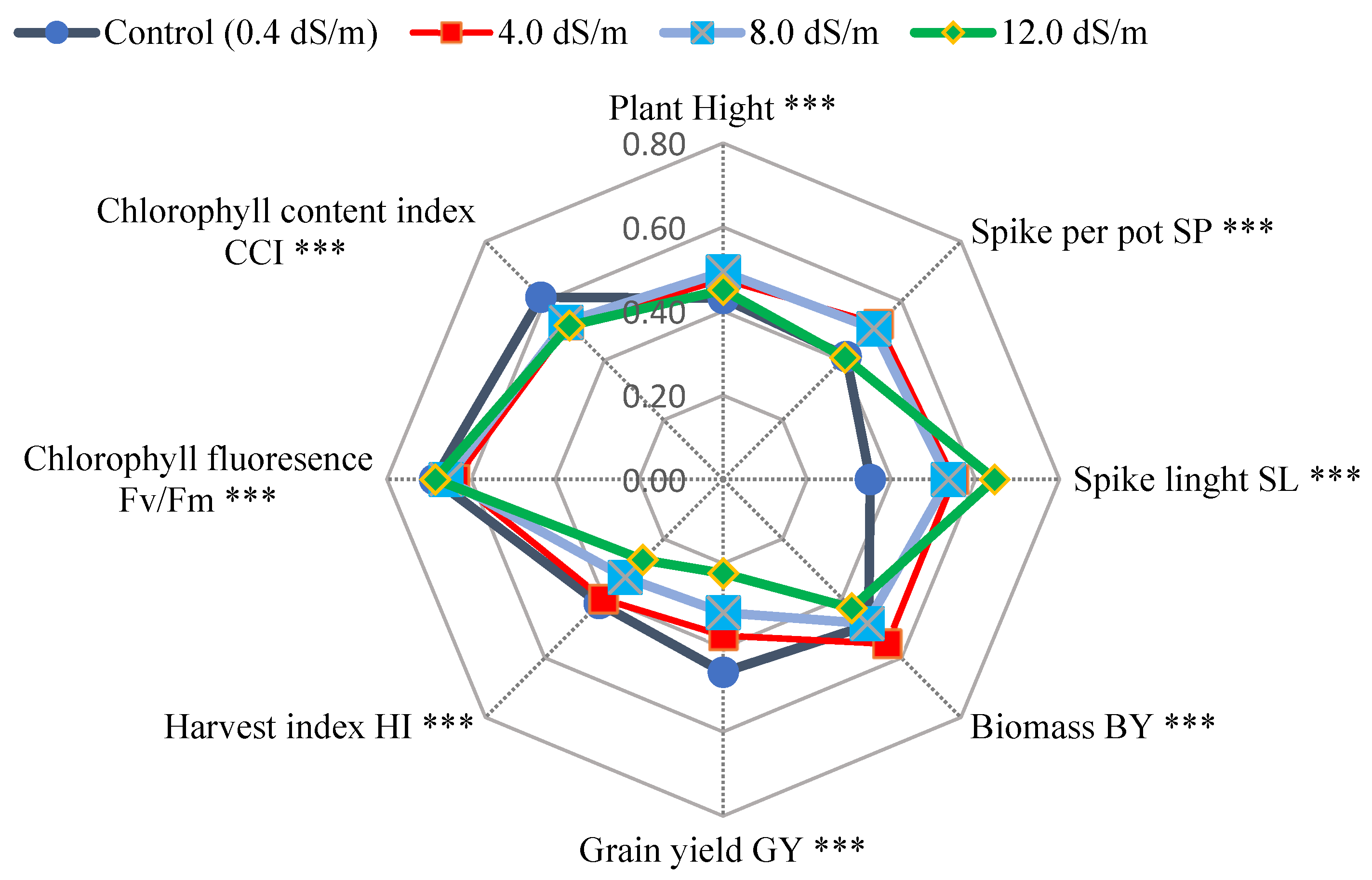
Averaged across forty wheat genotypes, the means of agronomic traits, e.g., grain yield gm per pot (GY), biomass gm per pot (BY), spikes per pot (SP), spike length in cm (SL), and harvest index % (HI), and measured physiological traits, chlorophyll fluoresce (Fv/Fm), and chlorophyll content index (CCI) under four salinity treatments (0.4, 4.0, 8.0 and 12.0 dS/m of seawater) are illustrated in Figure 1. GY and HI means were affected by the treatments gradually from 0.4 dS/m followed by 4.0, 8.0, and 12.0 dS/m as well as BY, with the exception of the control treatment, recorded the same mean of 8.0 dS/m. However, PH and Fv/Fm had almost the same performance. The control (0.4 dS/m) mean recorded was higher than other salinity treatments of CCI. In contrast, 4.0 and 8.0 dS/m means possessed similar values of SP and SL traits. Control and 12.0 dS/m behaved equally for SP, but they varied in SL. Additionally, the mean square of the genotype varied significantly (p < 0.001) for all studied traits as shown in Figure 1 and Table 4.

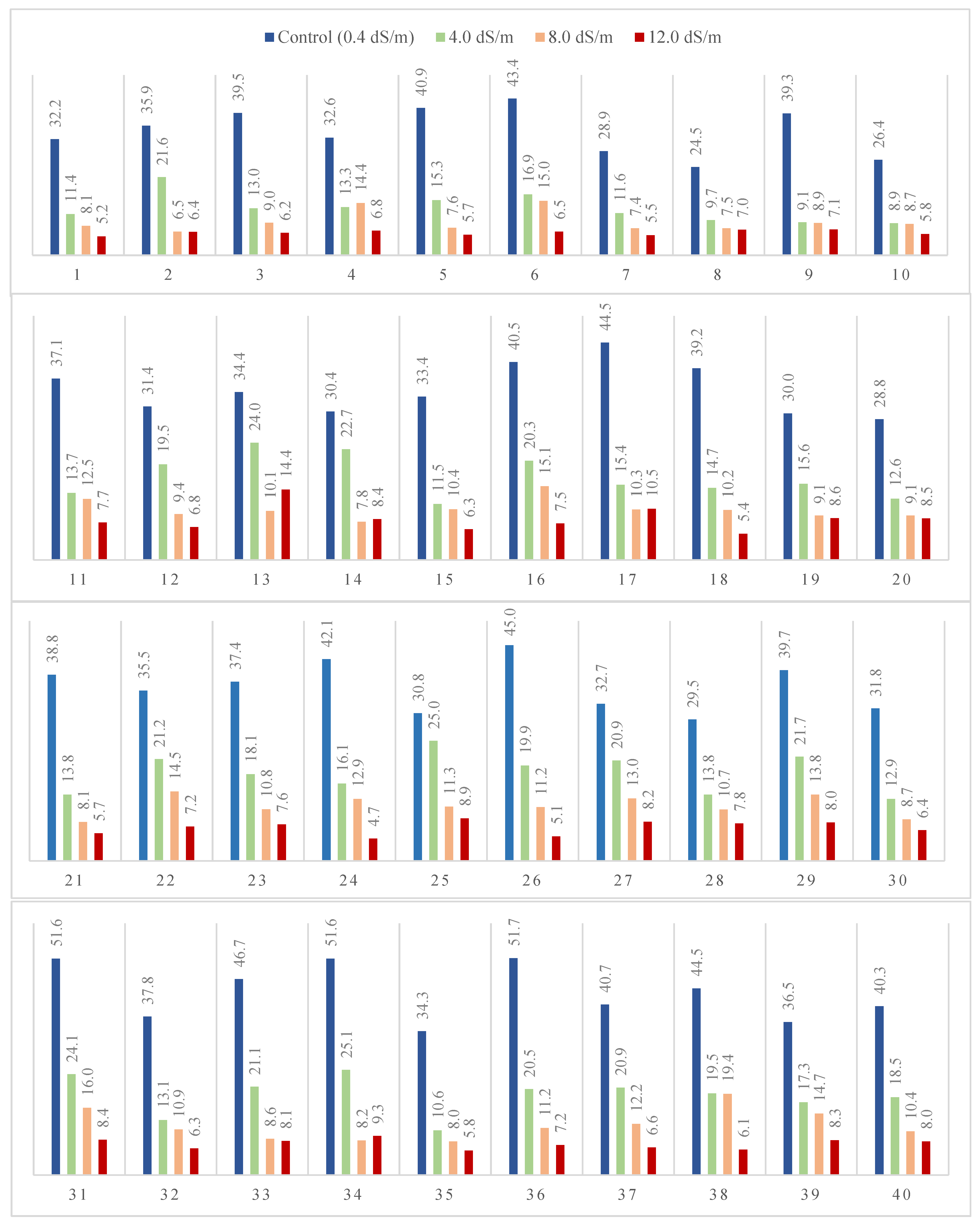
Figure 2 and Figure 3 and Table 5 and Table 6 show the grain yield mean performance of forty genotypes evaluated under four salinity treatments as well as combined data. In general, results indicate that forty genotypes decreased dramatically under salinity treatments in an orderly manner, from control followed by 4.0, 8.0, and 12.0 dS/m. Genotypes 31 and 34 had the highest values (25.0 and 22.6, respectively) in combined data over treatments Table 5 and Table 6. Moreover, 8.0 dS/m genotypes, 38 and 31 recorded 19.4 gm and 16.0 gm in comparison with the control. Additionally, genotypes 13 and 17 possess the highest values of 10.46 and 14.4 in 12.0 dS/m treatment. 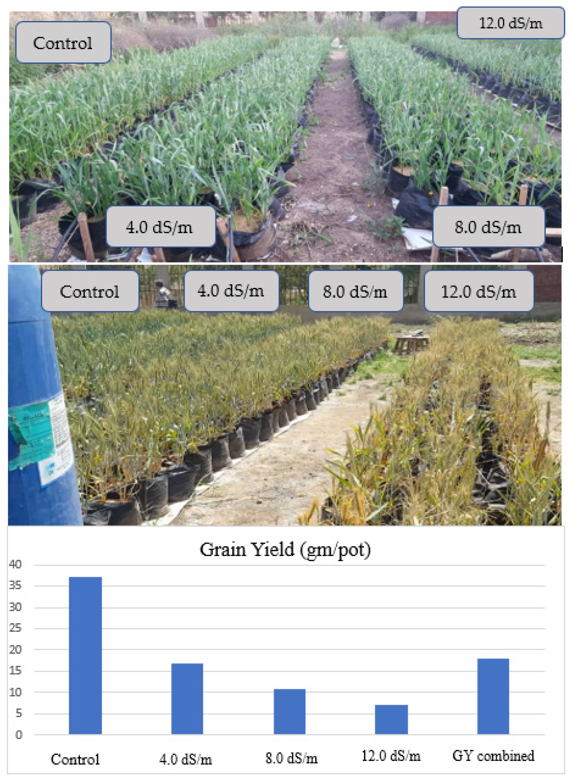Figure 7 reveals the mean of grain yield with the degradation from control followed by 4.0, 8.0, and 12.0 dS/m of forty genotypes evaluated in the pots experiment in bar plot and pictures, and the combined data analysis across all salinity treatments.

Table 5. Grain yield of control (GYN), grain yield at 8.0 dS/m (GY8), and salinity tolerance/susceptible indices of forty genotypes in 2019/20 season.

Genotype	GYN	GY8	TOL	GMP	STI	MP	HM	SSI
1	32.2^{† a–d}	8.1 ^cd	24.1	16.1	0.19	20.1	12.9	1.05
2	35.9 ^a–d	6.5 ^d	29.4	15.3	0.17	21.2	11.1	1.15
3	39.5 ^a–d	9.0 ^bcd	30.5	18.9	0.26	24.2	14.7	1.09
4	32.6 ^a–d	14.4 ^abc	18.2	21.7	0.34	23.5	20.0	0.78
5	40.9 ^a–d	7.6 ^cd	33.3	17.6	0.22	24.2	12.8	1.15
6	43.4 ^a–d	15.0 ^abc	28.4	25.6	0.47	29.2	22.3	0.92
7	28.9 ^bcd	7.4 ^cd	21.4	14.7	0.15	18.2	11.8	1.05
8	24.5 ^d	7.5 ^cd	17.0	13.5	0.13	16.0	11.5	0.98
9	39.3 ^a–d	8.9 ^bcd	30.4	18.7	0.25	24.1	14.5	1.09
10	26.4 ^cd	8.7 ^bcd	17.8	15.1	0.16	17.6	13.1	0.95
11	37.1 ^a–d	12.5 ^a–d	24.6	21.6	0.33	24.8	18.7	0.93
12	31.4 ^bcd	9.4 ^bcd	22.0	17.2	0.21	20.4	14.5	0.99
13	34.4 ^a–d	10.1 ^bcd	24.3	18.6	0.25	22.2	15.6	1.00
14	30.4 ^bcd	7.8 ^cd	22.5	15.4	0.17	19.1	12.5	1.04
15	33.4 ^a–d	10.4 ^bcd	23.0	18.7	0.25	21.9	15.9	0.97
16	40.5 ^a–d	15.1 ^abc	25.5	24.7	0.44	27.8	22.0	0.88
17	44.5 ^abc	10.3 ^bcd	34.2	21.4	0.33	27.4	16.8	1.08
18	39.2 ^a–d	10.2 ^bcd	29.0	20.0	0.29	24.7	16.2	1.04
19	30.0 ^bcd	9.1 ^bcd	20.9	16.5	0.20	19.6	14.0	0.98
20	28.8 ^bcd	9.1 ^bcd	19.7	16.2	0.19	19.0	13.8	0.96
21	38.8 ^a–d	8.1 ^cd	30.7	17.8	0.23	23.5	13.4	1.11
22	35.5 ^a–d	14.5 ^abc	21.0	22.7	0.37	25.0	20.6	0.83
23	37.4 ^a–d	10.8 ^bcd	26.6	20.1	0.29	24.1	16.7	1.00
24	42.1 ^a–d	12.9 ^a–d	29.1	23.3	0.39	27.5	19.8	0.97
25	30.8 ^bcd	11.3 ^bcd	19.4	18.7	0.25	21.1	16.6	0.89
26	45.0 ^abc	11.2 ^bcd	33.8	22.4	0.36	28.1	17.9	1.06
27	32.7 ^a–d	13.0 ^a–d	19.7	20.7	0.31	22.9	18.6	0.85
28	29.5 ^bcd	10.7 ^bcd	18.7	17.8	0.23	20.1	15.7	0.89
29	39.7 ^a–d	13.8 ^a–d	25.9	23.4	0.39	26.8	20.5	0.92
30	31.8 ^bcd	8.7 ^bcd	23.1	16.6	0.20	20.2	13.6	1.02
31	51.6 ^a	16.0 ^ab	35.5	28.8	0.59	33.8	24.5	0.97
32	37.8 ^a–d	10.9 ^bcd	27.0	20.3	0.30	24.4	16.9	1.00
33	46.7 ^ab	8.6 ^bcd	38.1	20.1	0.29	27.7	14.6	1.15
34	51.6 ^a	8.2 ^bcd	43.4	20.6	0.31	29.9	14.2	1.18
35	34.3 ^a–d	8.0 ^cd	26.3	16.6	0.20	21.2	13.0	1.08
36	51.7 ^a	11.2 ^bcd	40.5	24.1	0.42	31.5	18.4	1.10
37	40.7 ^a–d	12.2 ^a–d	28.5	22.3	0.36	26.4	18.8	0.99
38	44.5 ^abc	19.4 ^a	25.2	29.4	0.62	31.9	27.0	0.80
39	36.5 ^a–d	14.7 ^abc	21.8	23.1	0.38	25.6	20.9	0.84
40	40.3 ^a–d	10.4 ^bcd	29.8	20.5	0.30	25.4	16.6	1.04

^† Mean values within the same column for each trait with the same lower-case letter are not significantly different according to least significant difference (LSD) test at p ≤ 0.05. TOL, Tolerance index; MP, Mean productivity; STI, Stress tolerance index; GMP, Geometric mean productivity; HM, Harmonic mean stress; SSI, Susceptibility index.

Table 6. Grain yield of control (GYN), grain yield at 12.0 dS/m (GY12) treatment, and salinity tolerance/susceptible indices along with grain yield combined data (GYC) of forty genotypes in 2019/20 season.

Genotype	GYN	GY12	TOL	GMP	STI	MP	HM	SSI	GYC
1	32.2^{† a–d}	5.2 ^c	27.0	12.9	0.12	18.7	9.0	1.04	14.2 ^f–i
2	35.9 ^a–d	6.4 ^bc	29.5	15.2	0.17	21.2	10.9	1.02	17.6 ^b–i
3	39.5 ^a–d	6.2 ^bc	33.3	15.6	0.18	22.8	10.7	1.05	16.9 ^c–i
4	32.6 ^a–d	6.8 ^bc	25.8	14.9	0.16	19.7	11.2	0.98	16.8 ^c–i
5	40.9 ^a–d	5.7 ^bc	35.2	15.2	0.17	23.3	10.0	1.07	17.4 ^c–i
6	43.4 ^a–d	6.5 ^bc	36.9	16.8	0.20	25.0	11.4	1.05	20.5 ^a–e
7	28.9 ^bcd	5.5 ^bc	23.3	12.6	0.11	17.2	9.3	1.00	13.4 ^ghi
8	24.5 ^d	7.0 ^bc	17.4	13.1	0.12	15.8	10.9	0.88	12.2 ⁱ
9	39.3 ^a–d	7.1 ^bc	32.2	16.7	0.20	23.2	12.0	1.02	16.1 ^d–i
10	26.4 ^cd	5.8 ^bc	20.6	12.4	0.11	16.1	9.6	0.97	12.5 ^hi
11	37.1 ^a–d	7.7 ^bc	29.4	16.9	0.21	22.4	12.8	0.98	17.8 ^b–i
12	31.4 ^bcd	6.8 ^bc	24.6	14.6	0.15	19.1	11.1	0.97	16.8 ^c–i
13	34.4 ^a–d	14.4 ^a	20.0	22.5	0.36	24.4	20.3	0.72	20.7 ^a–e
14	30.4 ^bcd	8.4 ^bc	22.0	15.9	0.18	19.4	13.1	0.90	17.3 ^c–i
15	33.4 ^a–d	6.3 ^bc	27.1	14.5	0.15	19.9	10.6	1.01	15.4 ^d–i
16	40.5 ^a–d	7.5 ^bc	33.1	17.4	0.22	24.0	12.6	1.01	20.8 ^a–e
17	44.5 ^abc	10.5 ^ab	34.0	21.6	0.33	27.5	17.0	0.95	20.2 ^a–f
18	39.2 ^a–d	5.4 ^bc	33.9	14.5	0.15	22.3	9.4	1.07	17.4 ^b–i
19	30.0 ^bcd	8.6 ^bc	21.4	16.0	0.18	19.3	13.3	0.89	15.8 ^d–i
20	28.8 ^bcd	8.5 ^bc	20.3	15.7	0.18	18.7	13.2	0.87	14.8 ^e–i
21	38.8 ^a–d	5.7 ^bc	33.1	14.9	0.16	22.3	10.0	1.06	16.6 ^c–i
22	35.5 ^a–d	7.2 ^bc	28.3	15.9	0.18	21.3	11.9	0.99	19.6 ^a–f
23	37.4 ^a–d	7.6 ^bc	29.8	16.9	0.20	22.5	12.6	0.99	18.5 ^b–h
24	42.1 ^a–d	4.7 ^c	37.4	14.0	0.14	23.4	8.4	1.10	19.0 ^a–g
25	30.8 ^bcd	8.9 ^bc	21.9	16.5	0.20	19.8	13.8	0.88	19.0 ^a–g
26	45.0 ^abc	5.1 ^c	39.9	15.1	0.16	25.1	9.2	1.10	20.3 ^a–f
27	32.7 ^a–d	8.2 ^bc	24.6	16.4	0.19	20.5	13.1	0.93	18.7 ^b–g
28	29.5 ^bcd	7.8 ^bc	21.7	15.2	0.17	18.6	12.3	0.91	15.5 ^d–i
29	39.7 ^a–d	8.0 ^bc	31.7	17.8	0.23	23.9	13.3	0.99	20.8 ^a–e
30	31.8 ^bcd	6.4 ^bc	25.4	14.3	0.15	19.1	10.7	0.99	14.9 ^d–i
31	51.6 ^a	8.4 ^bc	43.2	20.8	0.31	30.0	14.5	1.04	25.0 ^a
32	37.8 ^a–d	6.3 ^bc	31.5	15.5	0.17	22.1	10.9	1.03	17.0 ^c–i
33	46.7 ^ab	8.1 ^bc	38.6	19.5	0.27	27.4	13.8	1.03	21.1 ^a–d
34	51.6 ^a	9.3 ^abc	42.3	21.9	0.35	30.5	15.8	1.02	23.6 ^ab
35	34.3 ^a–d	5.8 ^bc	28.5	14.2	0.14	20.1	10.0	1.03	14.7 ^e–i
36	51.7 ^a	7.2 ^bc	44.5	19.3	0.27	29.4	12.6	1.07	22.6 ^abc
37	40.7 ^a–d	6.6 ^bc	34.1	16.4	0.19	23.6	11.4	1.04	20.1 ^a–f
38	44.5 ^abc	6.1 ^bc	38.5	16.4	0.19	25.3	10.7	1.07	22.4 ^abc
39	36.5 ^a–d	8.3 ^bc	28.2	17.4	0.22	22.4	13.5	0.96	19.2 ^a–g
40	40.3 ^a–d	8.0 ^bc	32.2	18.0	0.23	24.2	13.4	0.99	19.3 ^a–g

^† Mean values within the same column for each trait with the same lower-case letter are not significantly different according to least significant difference (LSD) test at p ≤ 0.05; TOL, Tolerance index; MP, Mean productivity; STI, Stress tolerance index; GMP, Geometric mean productivity; HM, Harmonic mean stress; SSI, Susceptibility index.

Figure 2. Wheat grain yield gm per pot (GY) of forty genotypes evaluated in pot and grown under 0.4, 4.0, 8.0, or 12.0 dS/m of seawater in the 2019/20 season.

Figure 3. Bar chart of wheat genotypes grain yield gm per pot (GY) grown under 0.4, 4.0, 8.0, and 12.0 dS/m diluted seawater, and combined data over forty genotypes and photos representing the visual differences among the four saline treatments in 2019/20 season.

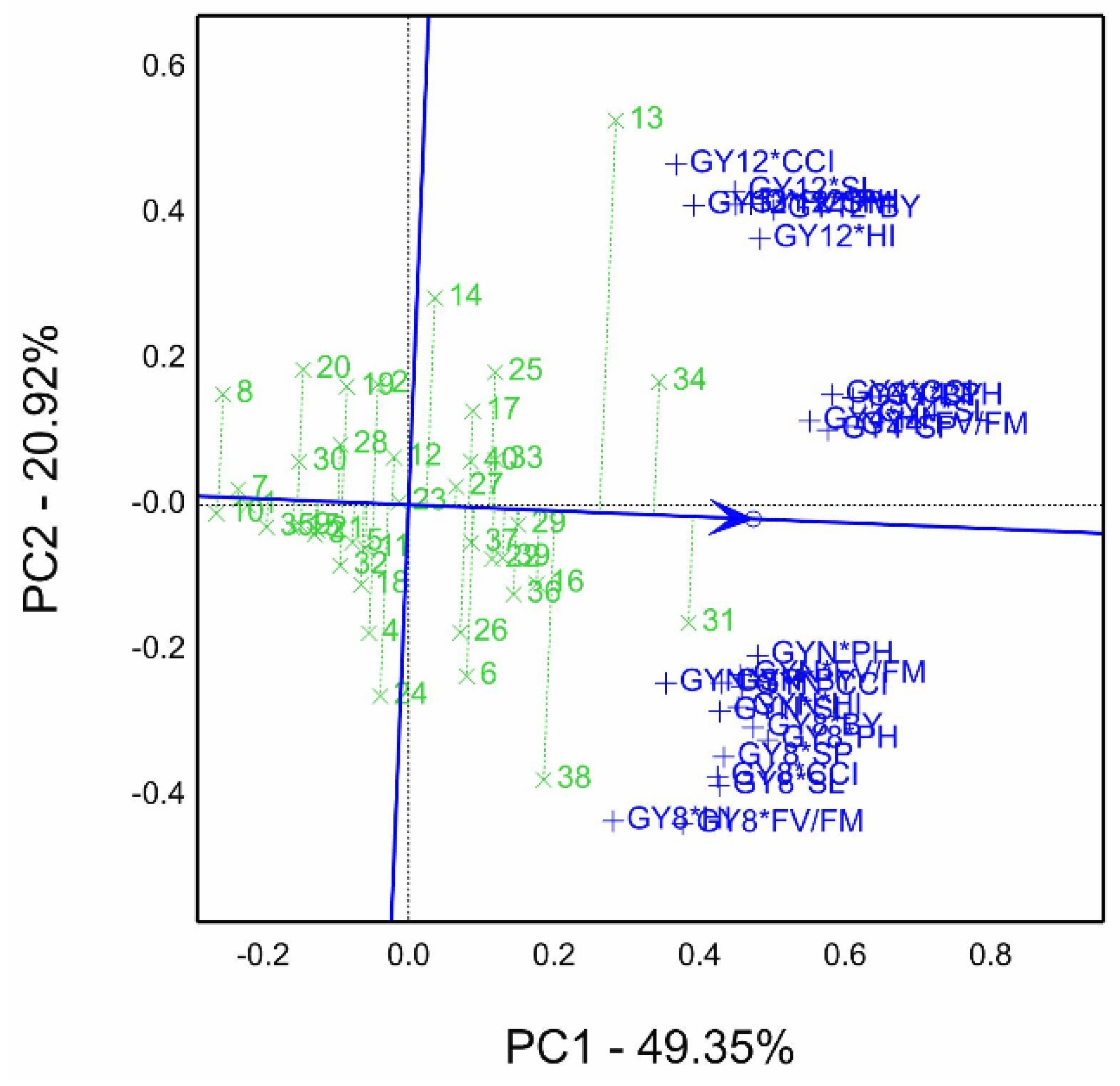
The combined means of genotypes by grain yield by all trait combinations (GY*T) evaluated under four salinity conditions (pot experiments) in the 2019/20 season is illustrated in Figure 4. Data were normalized to perform the GYT biplot, which accounted for 70.3% of total variation under four salinity levels. In the GYT biplot, the figure is divided into seven sectors, and the sector contains genotypes 13 and 34 on the polygon vertexes winner for GY12*CCI, HI, SL, BY, and GY4*BY, PH, SP, and Fv/Fm combinations. While genotype 31 is situated on the vertex of another sector with GYN*PH, CCI, Fv/Fm, BY, SL, and HI, and GY8*BY, PH, SP, SL, CCI. In the sector of genotypes 38 and 24 with combinations of GY8*HI and Fv/Fm.

Genotypes ranking based on GYT data is revealed in Figure 5. The order of genotype 31 > 34 > 13 > 38 > 16 > 36 > 29 joint with projection on average tester coordination (ATC blue line with arrow) and over grand mean (vertical line on ATC). However, genotypes 10 and 8 had the lowest performance of GYT combinations. Additionally, genotypes 31 and 34 had the best mean performance and stability; thus, they are close to the ATC line and combine the yield with all trait combinations (GY*T) evaluated under four salinity levels (pot experiments) in 2019/20 season. However, genotypes 13 and 38 are far away from ATC. Thus, they are unstable genotypes that rely on the GYT pattern of biplots.

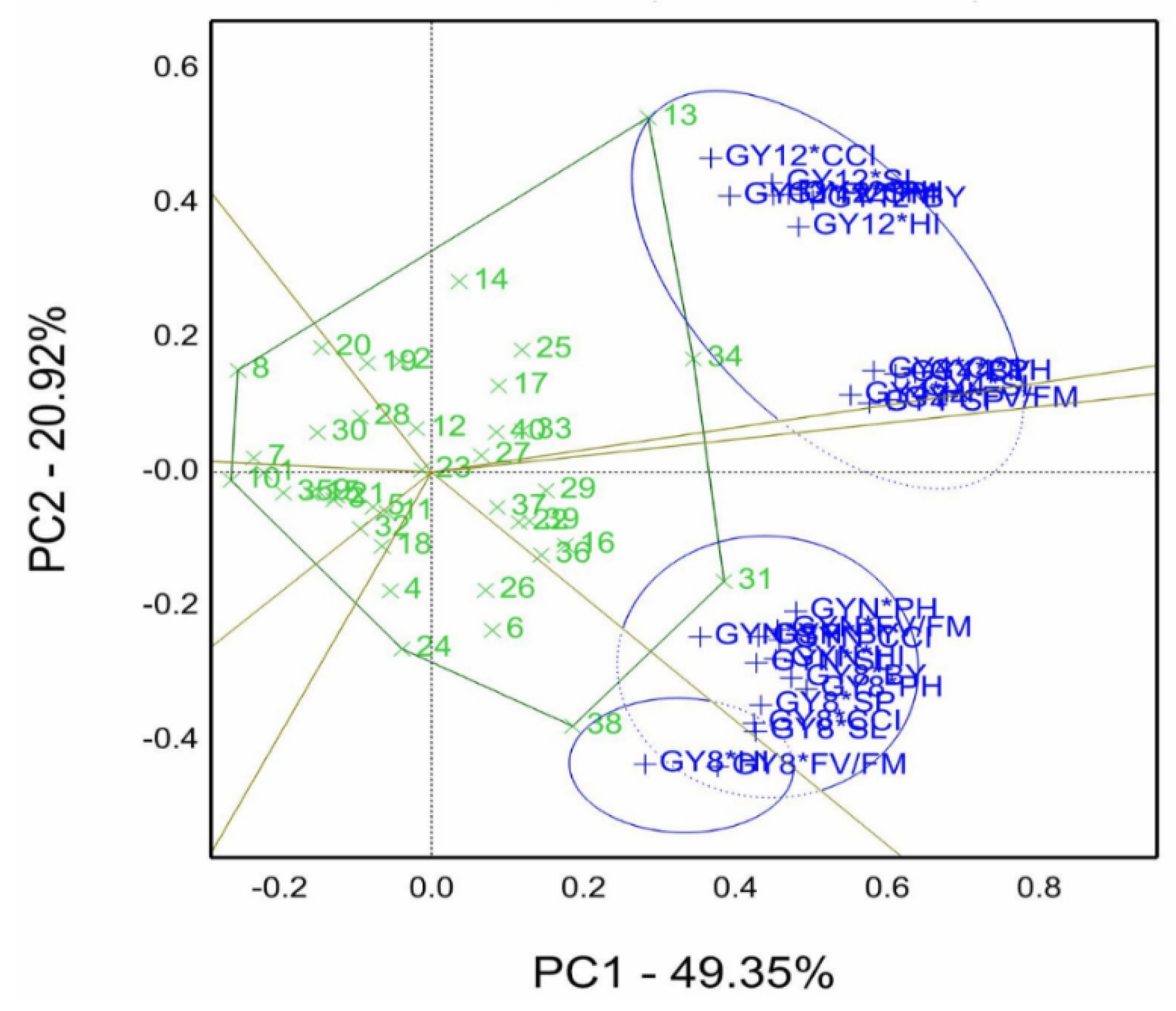
Salinity tolerance/susceptible indices (STI) calculated using grain yield gm per pot (GY) of control at 0.4 dS/m (GYN), grain yield at 8.0 dS/m (GY 8.0 dS/m), and grain yield at 12.0 dS/m (GY 12.0 dS/m) are shown in Table 3. In this study, data in Table 3 were used to estimate the graphical genotypes by traits model (GT) in Figure 6.

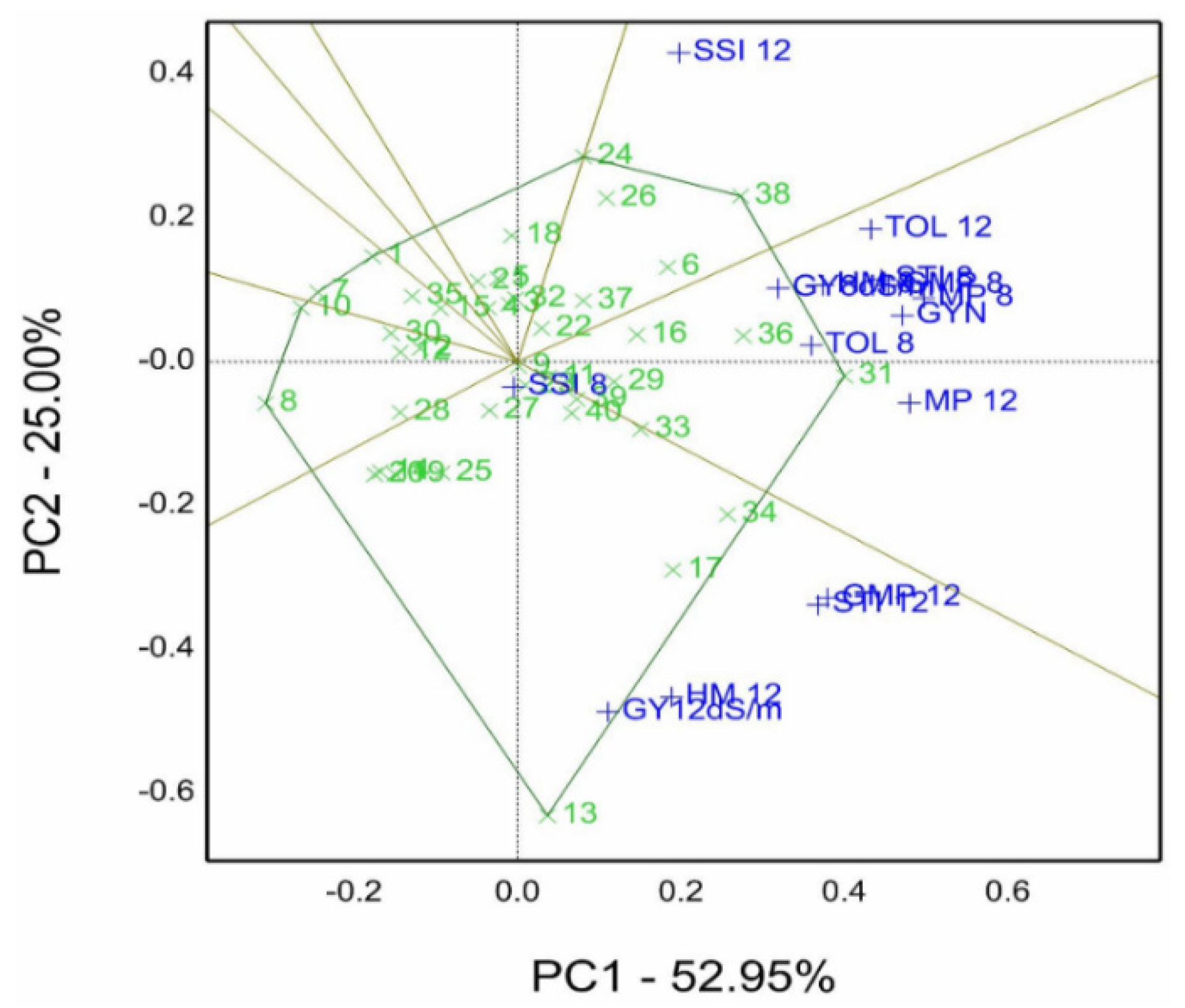
The sum of principal components PC1 and PC2 is 79.41% of the total variation of forty genotypes combined with STI, which is represented in figures in the titled genotype by salinity tolerance indices (GSTI) biplot. The findings helped to select genotypes 31 and 36, which are pointed on the vertex of the polygon in the sector containing GSTI, such as grain yield gm per pot of normal treatment (GYN), TOL8 (for 8.0 dS/m), TOL12 (for 12.0 dS/m), MP8, STI8, GMP8, MP12, STI12, HM8, and GY8. Additionally, genotype 13 is the winner of GY12, HM12, and GMP12 in its sector, but genotypes 24 and 26 situated in the sector had SSI8 and SSI12 as sensitive indies/genotypes.

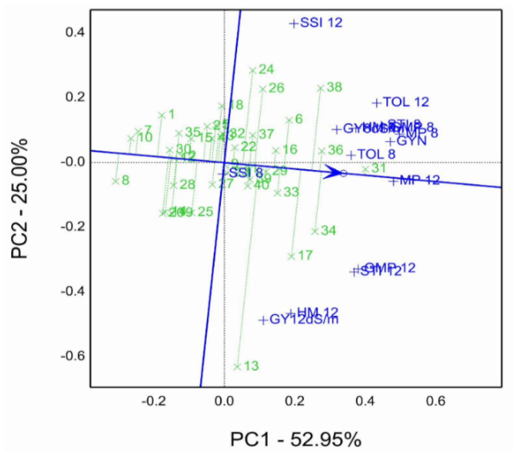
Means vs stability based on GSTI analysis divided from values in Table 5 and Table 6 and 6 of forty genotypes treated by four diluted seawaters in the 2019/20 season in pot trials, illustrated visually in Figure 7. Genotype 31, followed by 36, 34, 38, 17, 33, 6, and 16, recorded a high rank and stability for salinity tolerance indices. In contrast, genotype 8 had the lowest mean, and genotype 13 possessed the lowest stability referring to its long projection on ATC.

Figure 7. Mean vs. stability (GSTI) biplot of ranking genotypes based on grain yield gm per pot (GYN), grain yield gm per pot (GY 8.0, 12.0 dS/m), and salinity tolerance/susceptible indices (calculated at control with 0.4 dS/m, 8.0 dS/m, and 12.0 dS/m) of forty genotypes in the 2019/20 season. TOL, tolerance index; MP, mean productivity; STI, stress tolerance index; GMP geometric mean productivity; HM, harmonic mean; SSI, stress susceptibility index.

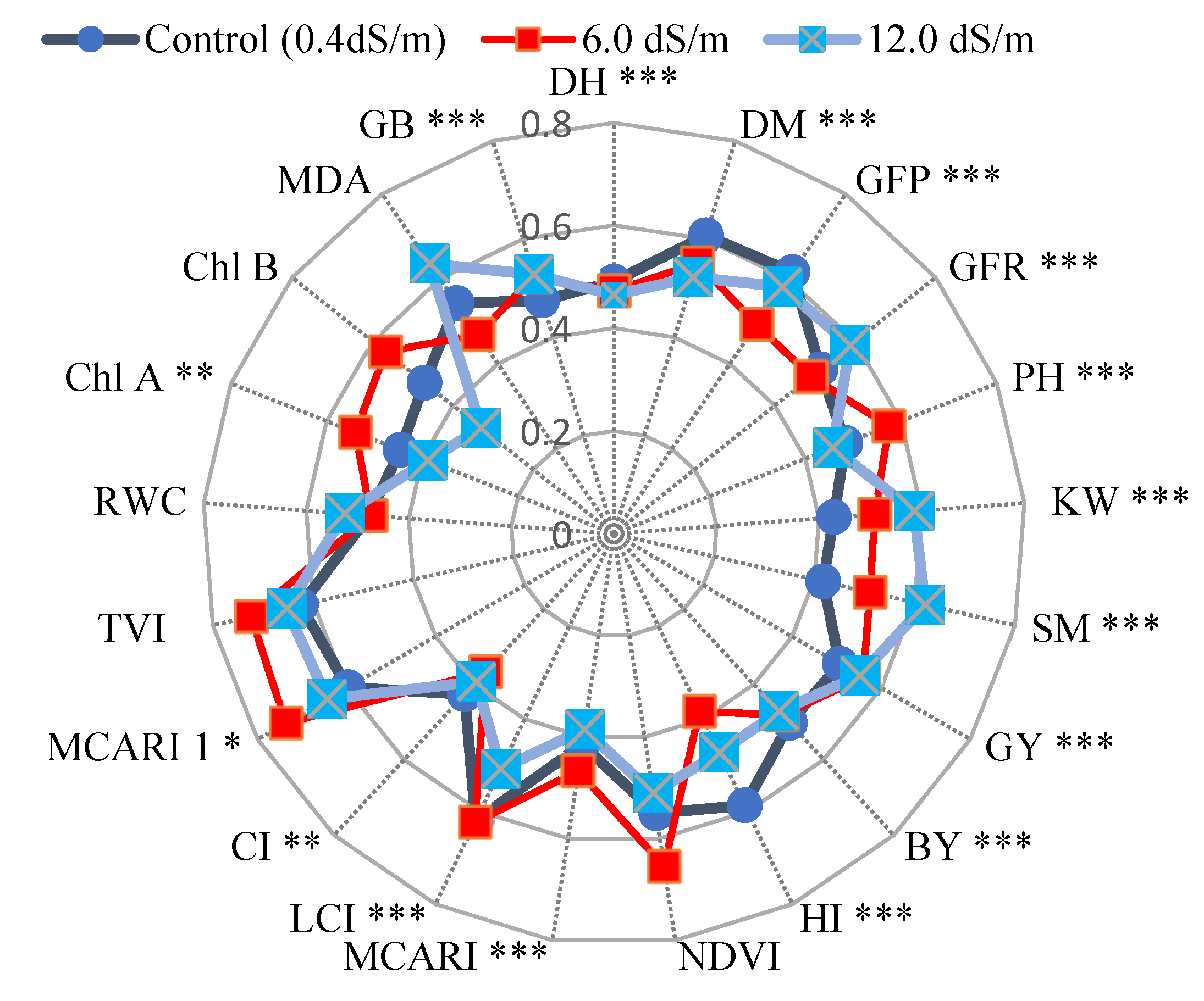
Agronomic and physiological traits, along with spectral reflectance indices (SRI), data were normalized to remove the effect of different units, in order to compare an averaged ten genotypes across three levels of salinity (seawater mitigation), e.g., control, 6.0 dS/m, and 12.0 dS/m. Figure 8 shows that traits such as GY, BY, DH, GB, CI, and RWC recorded almost the same mean performance under three salinity levels. However, traits like KW, SM, GFR, TVI, and MCARI possess high mean values of 6.0 dS/m and 12.0 dS/m in comparison with the control. Additionally, control of traits DM, GFP, and HI tend to be higher than 6.0 dS/mor 12 dS/m. In contrast, control of traits Chl A, B, PH, and MDA is situated in between other treatments. The genotype component of the source of variation for all traits varied differences significantly (p < 0.01), with the exception of TVI1, RWC, Chl B, NDVI, shown in Table 7 and Figure 8.

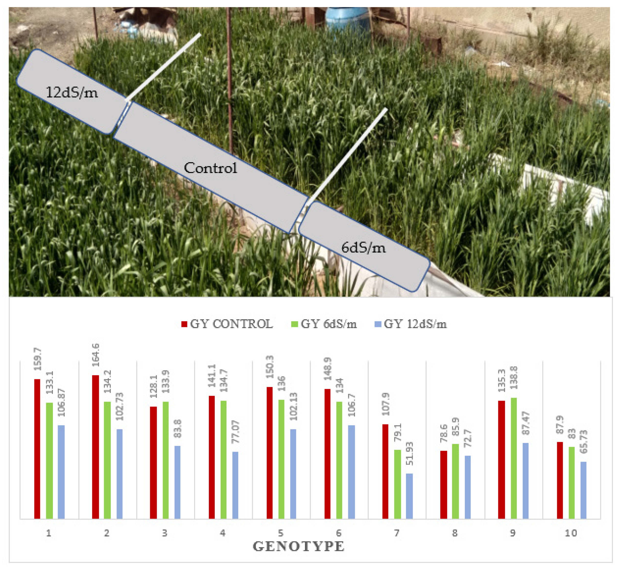
Figure 9 and Table 8 show the grain yield gm per row (GY) mean performance of ten genotypes evaluated in a simulated lysimeter and irrigated with 0.4, 6.0, and 12.0 dS/m diluted seawater. The data represent genotypes classified into two categories, i.e., genotypes 1, 2, 3, 4, 5, 6, and 9 (Misr 4) recorded as high performance, while the old varieties, i.e., genotypes 7 (Kharchia 65), 8 (Oasis F86), and 10 (Sakha 8) under 3 saline irrigation were not. In addition, in the combined analysis, genotypes, 1 and 2 recorded the highest values of 133.3 and 133.8 g, respectively. However, varieties 7, 8, and 10 had 79.6, 79.1, and 78.9, respectively, shown in Table 8.

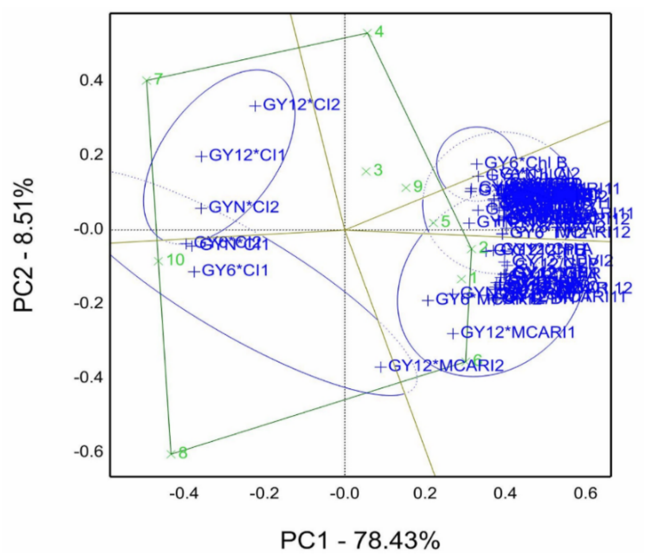
Genotype by grain yield*traits (GYT) pattern was used to select the best one from ten genotypes evaluated in a simulated lysimeter in the 2020/21 season illustrated in Figure 10. The GYT biplot accounted for 86.94% of the total variation. Moreover, the sector of genotypes 2 and 6 had the most combinations of agronomic and physiological traits and spectral reflectance indices. The sector of genotypes 8 and 10 had combinations of GY6*CI1, CI2, and GYN*CI1, while the sector of genotype 7 contains GYN*CI2, GY12*CI1, and CI2. Thus, the best genotypes that rely on this view are genotypes 2 and 6.

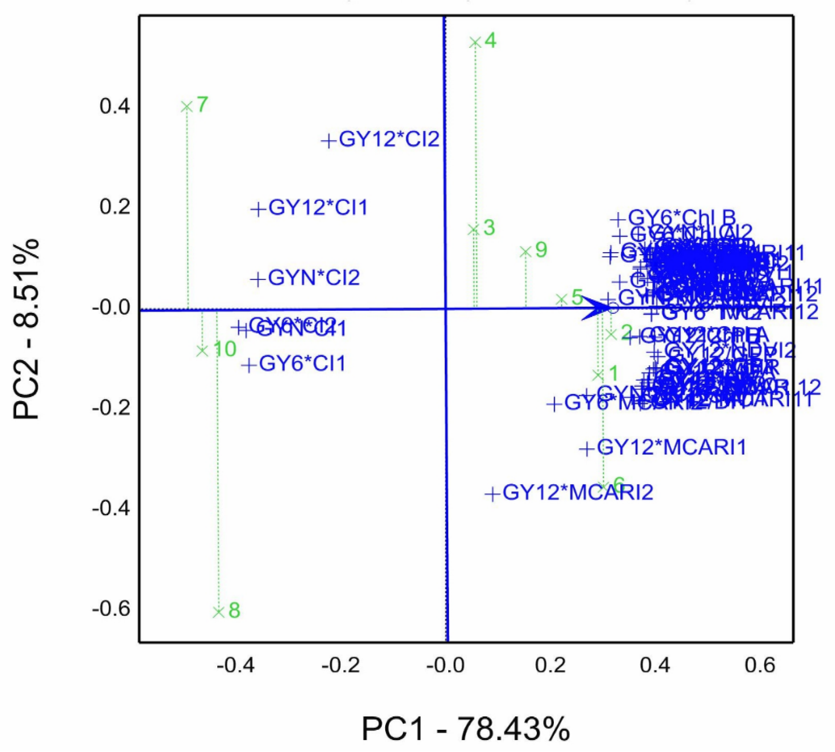
Based on the GYT model graphical analysis, ten entries were evaluated under three salinity treatments by simulated lysimeter in the 2020/21 season, as shown in Figure 11. The genotypes rank is 2 > 6>1 > 5>9 > 4>8 > 10 > 7 joint with projection on average tester coordination (ATC blue line with arrow). Additionally, genotypes 2, 1, and 5 would be the best mean performance and stability; thus, they are close to the ATC line and combine the yield with all trait combinations (GY*T). However, genotypes 6 and 4 are far away from the ATC, thus they are unstable genotypes.

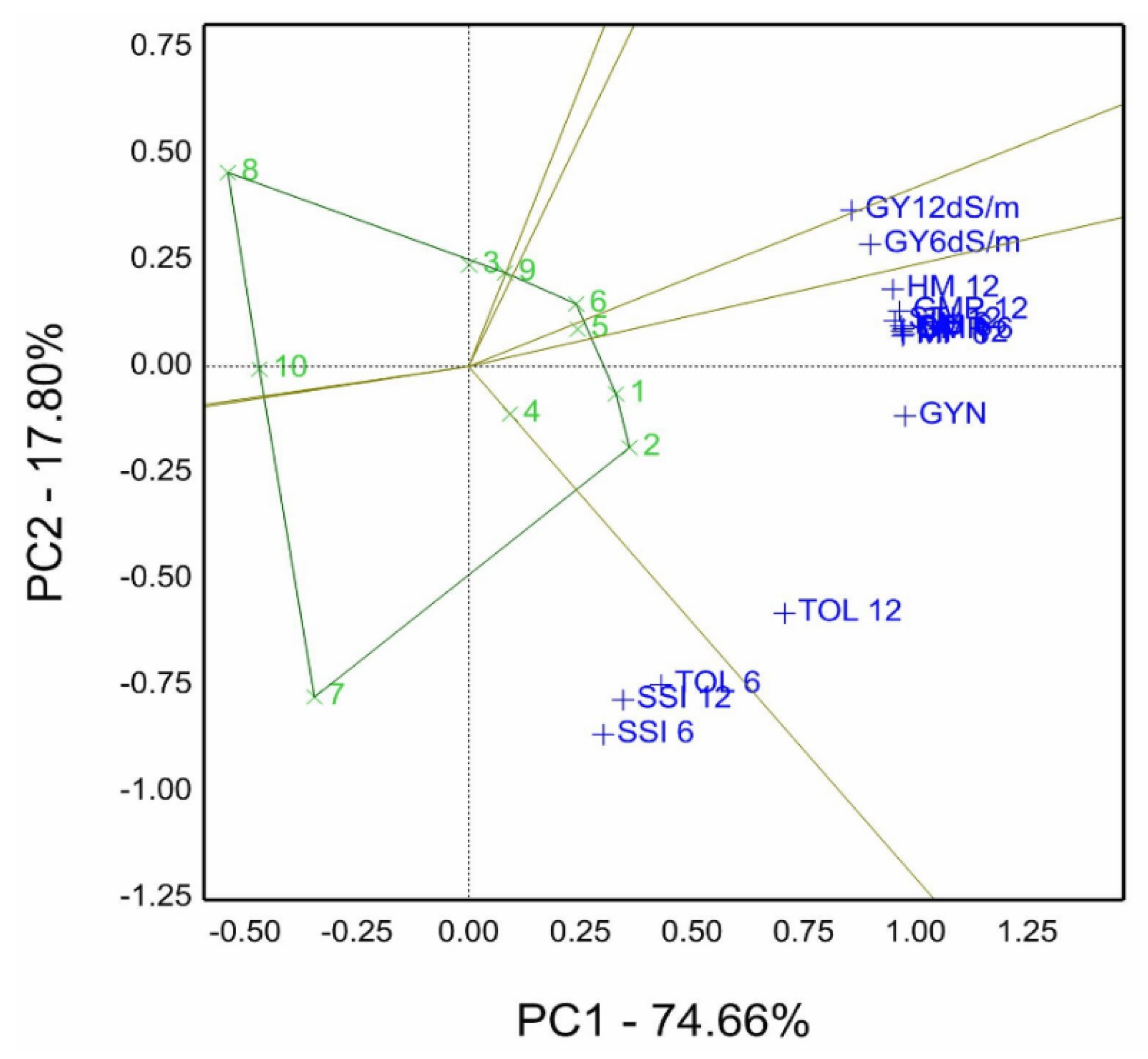
Relying on the genotype by trait (GT) biplot pattern, we compute salinity tolerance/sensitive indices (STI) using grain yield of control gm per row (GYN), grain yield of 6.0 dS/m (GY6 dS/m), grain yield of 12.0 dS/m gm per row (GY12 dS/m), and another STI of ten genotypes in Table 4. In this study, we performed data in Table 4 to depict graphical genotypes by traits model (GT) in Figure 12. The sum of principal components was 93.11% of the total variation for ten genotypes combined with STI, represented in figures termed genotype by salinity tolerance indices (GSTI) biplot. The findings indicate that genotypes 1 and 2 are located on the polygon’s vertex in its sector containing GSTI combinations such as grain yield normal gm per row (GYN), TOL12 (for 12.0 dS/m), HM12, MP6, STI6, GMP6, MP12, STI12, HM6, GMP12, and GYC combined. Additionally, genotype 7 is the winner of TOL6 (for 6.0 dS/m), SSI6, and SSI12. However, genotype 6 is the winner in its sector for GY12 dS/m.

Based on the means vs stability GSTI biplot, ten entries evaluated under three salinity treatments by simulated lysimeter in the 2020/21 season are illustrated in Figure 13. The rank commences from genotype 2 followed by 1, 5, 6, and 4 placed on the average tester coordination line (ATC blue line with an arrow). Additionally, genotypes 2 and 1 would show the best mean performance and stability. However, genotypes 7 and 8 are far away from the ATC; thus, they are unstable genotypes.

4. Discussion

The genotype by yield*trait (GYT) biplots approach, as proposed by Yan and Frégeau–Reid [46], graphically identified the relationship between genotypes and studied traits, specifically, in the case of large genotype numbers and characters. For example, in salinity and drought stress conditions with contrasting regimes. Additionally, these methodologies can be used by breeders to select the elite genotypes not only had grain yield performance but also combined with other trait combinations. For instance, the selection for barley drought tolerance reported by [47,49], wheat rusts resistance selected using genotype*traits (GT) technique by the researchers [48], the authors [65] selected common bean genotypes using the GYT model, and the researchers identified durum wheat drought tolerance evaluated in multi-years under rainfed conditions using GYT [51]. In our study, we evaluated forty bread wheat genotypes irrigated by four diluted seawater levels in the pot experiments to select six genotypes (i.e., 6, 16, 31, 33, 34, 36) in the first season based on results shown in Figure 2 and Figure 6. To evaluate wheat genotypes grown under three saline levels, lysimeter experiments were conducted in the second season to compare the performance of 10 wheat genotypes and varieties, i.e., three old varieties i.e., 7, 8, 10 (Kharchia 65, Oasis F86, and Sakha 8, respectively) along with new cultivar genotype 9 (Misr 4) for comparison with 6 other wheat genotypes. Genotypes 2 and 1 were selected, which might be salinity tolerance genotypes, as the outcome of these experiments are shown in Figure 11 and Figure 13.

The wheat grain-filling stage provides the most informative measurements using spectral reflectance indices (SRIs) [35]. Thus, more genotypic variation was detected than for early growth vegetation and heading [35]. On the contrary, ref. [9] reported significant differences in genotypes, salinity treatments, growth stages, years, and their interactions for all vegetation SRIs and water SRIs. The SRI scores detected significant differences for quinoa genotypes and contrasting water regimes [27]. Nonetheless, the SRIs in one of the locations studied (irrigated and non-irrigated) did not differ among genotypes, which may refer to the closeness of the plants ripening. In our study, reflectance indices such as MACRI 1, LCI1, and CI 1 in the first measurement, as well as all SRIs in the second reading, recorded that the genotypes significantly varied (Table 7). The results of the combination of GYT with SRIs in Figure 10 and Figure 11 confirmed that genotypes 2 and 1 are the best salinity tolerance genotypes from this view and GSTI view of salinity tolerance indices in Figure 12 and Figure 13. In this study, we used GT and GYT approaches to select the superior genotypes not only based on grain yield but also other physiological traits such as amino acid glycine betaine and chlorophyll fluorescence (Fv/Fm) and chlorophyll content index (CCI), as well as agronomic traits such as PH, HI, and BY. These findings are in agreement with the results described by other reports [9,27,66,67].

In the 2019/20 season, forty genotypes were evaluated together under four salinity treatments. This large number might have created significant variations by interaction with treatments, interpreted by the coefficient of variation (CV) of GY (32.4%), as shown in Table 4. Thus, in the second season we reduced the number to ten genotypes but added the old varieties, i.e., 7, 8, 10 (Kharchia65, Oasis F86, and Sakha 8, respectively), whose low achieved GY might refer to their yield potential, even with rusts fungicide applied (Figure 9; Table 7). The approach of GYT was used with agronomic and physiological traits and spectral reflectance indices to select the best genotypes. Figure 3 and Figure 10 identified more than thirteen combinations for genotype 31 and the other combinations situated in the sector of genotypes 34 and 13 (however, 13 was unstable, as shown in Figure 5). Moreover, genotypes 2 and 6 in the second season had several combinations of spectral reflectance indices (SRI) (Figure 10). These results were similar to those found by others [66,68,69].

Additionally, GT models suggested by [45] were used to identify and rank genotypes based on salinity tolerance/susceptible indices (GSTI), genotypes 6, 16, 31, 33, 34, and 36 were selected in the first season in pot experiments, and genotypes 2 and 1 were selected in lysimeter experiments as superior genotypes in the second season (Figure 7 and Figure 13). However, it is hard to select genotypes 13 and 8, as shown in Figure 7, as well as genotypes 7 and 8, shown in Figure 13, which are unstable and had low performance. These findings are consistent with others [50] who performed the GT technique to select the elite rice entry [13] using principal component analyses (PCA). Moreover, other reports [49] used genotype by yield stress index (GYSI) to select the best genotypes that had drought tolerance.

Both experiments used a radar chart to examine the studied characters’ relationship and genotype means. For example, GY and HI were gradually affected by salinity treatment (Figure 1 and Figure 8). Additionally, genotypes varied significantly for all traits in the first season (Figure 1 and Table 7). All agronomic, physiological traits, and spectral reflectance indices, are shown in Figure 8 and Table 7. Similarly, findings of nitrogen starvation treatments did not impact on Fv/Fm ratio [70]. While the same trend of GY is affected positively by sowing depth [71]. Other reports [72] stated that genotype clusters had varied responses to salinity levels in several traits, such as SL. Additionally, water stress treatment benefited winter wheat growth using subsurface drip irrigation of GY, HI and BY in the second season [72,73].

5. Conclusions

The two evaluation systems (pots and lysimeters) were effective in discriminating wheat plant materials tested for salt tolerance. Genotype by yield*trait (GYT) and genotype by traits (GT) approaches were supportive in facilitating genotype selection based on grain yield and other associated traits (agronomic, physiological traits, and SRI combinations) as well as stress tolerance indices. This study showed that genotypes 6, 16, 31, 33, 34, and 36 in the 2019/20 season (a large number of genotypes might be creating interaction by treatments) and genotypes 2 (16) and 1 (6) performed better than Kharchia 65 and Sakha 8 (low yielding and old varieties) in the second season of 2020/21, which were selected as superior genotypes. Thus, it can be recommended to sow those selected genotypes in salt-affected soils and involve them in wheat breeding programs. It could be concluded that spectral reflectance indices performed effectively in detecting the genotypic variation. For future work based on these findings, it is suggested that these selected genotypes could be used to release a new salinity tolerance variety and exploit these plant materials to make new hybridizations used in the wheat breeding program for salinity.

Author Contributions

Conceptualization, A.M.S.E., M.A.D. and M.T.A.; investigation, A.M.S.E., M.A.D., A.I.S., M.M.A.S., O.M.A.E., R.A.K., A.M.A.; statistical designs and analyses, A.M.S.E.; writing—original draft preparation, A.M.S.E., M.A.D.; writing—review and editing A.M.S.E., M.T.A.; All authors have read and agreed to the published version of the manuscript.

Funding

This research received no external funding.

Data Availability Statement

The authors state that all data generated or analyzed during this study are included in this article. The full data used to support the findings of this study are available from the corresponding author upon request.

Acknowledgments

This work was supported by Wheat Research Department, Field Crops Research Institute, Agricultural Research Center, Giza, Egypt.

Conflicts of Interest

The authors declare no conflict of interest.

Abbreviations

GYT	genotype by yield*trait
GT	genotype by traits
GSTI	Genotype by salinity tolerance indices
SRI	spectral reflectance indices
CCI	chlorophyll content index
Fv/Fm	chlorophyll fluorescence
GY	grain yield
PH	plant height
HI	harvest index
MDA	malondialdehyde
GB	Glycine betaine

References

Reynolds, M.P.; Braun, H.-J. Wheat Improvement. In Wheat Improvement Food Security in a Changing Climate; Reynolds, M.P., Braun, H.-J., Eds.; Springer: Cham, Switzerland, 2022; pp. 3–15. ISBN 9783030906733. [Google Scholar]
Moustafa, E.S.A.; Ali, M.M.A.; Kamara, M.M.; Awad, M.F.; Hassanin, A.A.; Mansour, E. Field Screening of Wheat Advanced Lines for Salinity Tolerance. Agronomy 2021, 11, 281. [Google Scholar] [CrossRef]
Quamruzzaman, M.; Manik, S.; Livermore, M.; Johanson, P.; Zhou, M.; Shabala, S. Multidimensional Screening and Evaluation of Morpho- Physiological Indices for Salinity Stress Tolerance in Wheat. J. Agron. Crop Sci. 2022, 208, 454–471. [Google Scholar] [CrossRef]
Morsy, S.; Elbasyoni, I.S.; Baenziger, S.; Abdallah, A.M. Gypsum Amendment Influences Performance and Mineral Absorption in Wheat Cultivars Grown in Normal and Saline-Sodic Soils. J. Agron. Crop Sci. 2022, 208, 675–692. [Google Scholar] [CrossRef]
Afridi, M.S.; Amna; Sumaira; Mahmood, T.; Salam, A.; Mukhtar, T.; Mehmood, S.; Ali, J.; Khatoon, Z.; Bibi, M.; et al. Induction of Tolerance to Salinity in Wheat Genotypes by Plant Growth Promoting Endophytes: Involvement of ACC Deaminase and Antioxidant Enzymes. Plant Physiol. Biochem. 2019, 139, 569–577. [Google Scholar] [CrossRef]
Ghonaim, M.M.; Mohamed, H.I.; Omran, A.A.A. Evaluation of Wheat (Triticum aestivum L.) Salt Stress Tolerance Using Physiological Parameters and Retrotransposon-Based Markers. Genet. Resour. Crop Evol. 2021, 68, 227–242. [Google Scholar] [CrossRef]
Aycan, M.; Baslam, M.; Asiloglu, R.; Mitsui, T.; Yildiz, M. Development of New High-Salt Tolerant Bread Wheat (Triticum aestivum L.) Genotypes and Insight into the Tolerance Mechanisms. Plant Physiol. Biochem. 2021, 166, 314–327. [Google Scholar] [CrossRef]
Jamil, A.; Riaz, S.; Ashraf, M.; Foolad, M.R. Gene Expression Profiling of Plants under Salt Stress. CRC Crit. Rev. Plant Sci. 2011, 30, 435–458. [Google Scholar] [CrossRef]
Shabala, S.; Bose, J.; Hedrich, R. Salt Bladders: Do They Matter? Trends Plant Sci. 2014, 19, 687–691. [Google Scholar] [CrossRef]
Mohamed, N.N. Management of Salt-Affected Soils in the Nile Delta. In Handbook of Environmental Chemistry; Springer: Cham, Switzerland, 2017; Volume 55, pp. 265–295. [Google Scholar]
El-Hendawy, S.; Al-suhaibani, N.; Mubushar, M.; Tahir, M.U.; Marey, S.; Refay, Y.; Tola, E. Combining Hyperspectral Reflectance and Multivariate Regression Models to Estimate Plant Biomass of Advanced Spring Wheat Lines in Diverse Phenological Stages under Salinity Conditions. Appl. Sci. 2022, 12, 1983. [Google Scholar] [CrossRef]
Rehman, H.U.; Alharby, H.F.; Bamagoos, A.A.; Abdelhamid, M.T.; Rady, M.M. Sequenced Application of Glutathione as an Antioxidant with an Organic Biostimulant Improves Physiological and Metabolic Adaptation to Salinity in Wheat. Plant Physiol. Biochem. 2021, 158, 43–52. [Google Scholar] [CrossRef]
Sardouie-Nasab, S.; Nejad, M.G.; Nakhoda, B. Field Screening of Salinity Tolerance in Iranian Bread Wheat Lines. Crop Sci. 2014, 54, 1489–1496. [Google Scholar] [CrossRef] [Green Version]
Awad, N.M.; Turky, A.S.; Abdelhamid, M.T.; Attia, M. Ameliorate of Environmental Salt Stress on the Growth of Zea mays L. Plants by Exopolysaccharides Producing Bacteria. J. Appl. Sci. Res. 2012, 8, 2033–2044. [Google Scholar]
Dawood, M.G.; Abdelhamid, M.T.; Schmidhalter, U. Potassium Fertiliser Enhances the Salt-Tolerance of Common Bean (Phaseolus vulgaris L.). J. Hortic. Sci. Biotechnol. 2015, 89, 185–192. [Google Scholar] [CrossRef]
Nassar, R.M.A.; Kamel, H.A.; Ghoniem, A.E.; Alarcón, J.J.; Sekara, A.; Ulrichs, C.; Abdelhamid, M.T. Physiological and Anatomical Mechanisms in Wheat to Cope with Salt Stress Induced by Seawater. Plants 2020, 9, 237. [Google Scholar] [CrossRef] [Green Version]
FAOSTAT. Available online: https://www.fao.org/worldfoodsituation/csdb/en/ (accessed on 14 June 2022).
Ashraf, M. Biotechnological Approach of Improving Plant Salt Tolerance Using Antioxidants as Markers. Biotechnol. Adv. 2009, 27, 84–93. [Google Scholar] [CrossRef]
Gizaw, S.A.; Jayfred Gaham, V.; Godoy, K.G.-C.; Carter, A.H. Using Spectral Reflectance Indices as Proxy Phenotypes for Genome-Wide Association Studies of Yield and Yield Stability in Pacific Northwest Winter Wheat. Crop Sci. 2018, 58, 1232–1241. [Google Scholar] [CrossRef]
Khush, G.S. Strategies for Increasing the Yield Potential of Cereals: Case of Rice as an Example. Plant Breed. 2013, 132, 433–436. [Google Scholar] [CrossRef]
Richards, R.A. Selectable Traits to Increase Crop Photosynthesis and Yield of Grain Crops. J. Exp. Bot. 2000, 51, 447–458. [Google Scholar] [CrossRef]
Esfandiari, E.; Shekari, F. The Effect of Salt Stress on Antioxidant Enzymes’ Activity and Lipid Peroxidation on the Wheat Seedling Physiology of Environmental Stresses on Crop Plants View Project. Not. Bot. Horti Agrobot. Cluj-Napoca 2007, 35, 48–56. [Google Scholar] [CrossRef]
Borzouei, A.; Kafi, M. Long Term Salinity Stress in Relation to Lipid Peroxidation, Super Oxide Dismutase Activity and Proline Content of Salt-Tolerant Wheat Cultivars Nitrification Inhibitor View Project Rural Empowerment and Agro-Tourism, Environmental Assessment of Ecotourism Area View Project. Chil. J. Agric. Res. 2012, 72, 476–482. [Google Scholar]
Chen, H.; Jiang, J.G. Osmotic Adjustment and Plant Adaptation to Environmental Changes Related to Drought and Salinity. Chil. J. Agric. Res. 2012, 74, 309–319. [Google Scholar] [CrossRef]
Rabbani, G.; Choi, I. Roles of Osmolytes in Protein Folding and Aggregation in Cells and Their Biotechnological Applications. Int. J. Biol. Macromol. 2018, 109, 483–491. [Google Scholar] [CrossRef] [PubMed]
Gizaw, S.A.; Garland-Campbell, K.; Carter, A.H. Use of Spectral Reflectance for Indirect Selection of Yield Potential and Stability in Pacific Northwest Winter Wheat. Field Crops Res. 2016, 196, 199–206. [Google Scholar] [CrossRef] [Green Version]
Hinojosa, L.; Kumar, N.; Gill, K.S.; Murphy, K.M.; Crop, D. Spectral Reflectance Indices and Physiological Parameters in Quinoa under Contrasting Irrigation Regimes. Crop Sci. 2019, 59, 1927–1944. [Google Scholar] [CrossRef] [Green Version]
Sun, H.; Feng, M.; Xiao, L.; Id, W.Y.; Wang, C.; Jia, X.; Zhao, Y.; Zhao, C.; Muhammad, S.K.; Li, D. Assessment of Plant Water Status in Winter Wheat (Triticum aestivum L.) Based on Canopy Spectral Indices. PLoS ONE 2019, 10, e0216890. [Google Scholar] [CrossRef]
Bruning, B.; Berger, B.; Lewis, M.; Liu, H.; Garnett, T. Approaches, Applications, and Future Directions for Hyperspectral Vegetation Studies: An Emphasis on Yield-Limiting Factors in Wheat. Plant Phenome J. 2020, 3, e20007. [Google Scholar] [CrossRef]
Fiorani, F.; Rascher, U.; Jahnke, S.; Schurr, U. Imaging Plants Dynamics in Heterogenic Environments. Curr. Opin. Biotechnol. 2012, 23, 227–235. [Google Scholar] [CrossRef]
Reynolds, M.P.; Pask, A.J.D.; Mullan, D.M. Physiological Breeding I: Interdisciplinary Approaches to Improve Crop; CIMMYT: Mexico City, Mexico, 2012. [Google Scholar]
Jackson, R.D.; Ezra, C.E. Spectral Response of Cotton to Suddenly Induced Water Stress. Int. J. Remote Sens. 2010, 6, 177–185. [Google Scholar] [CrossRef]
Babar, M.A.; Reynolds, M.P.; van Ginkel, M.; Klatt, A.R.; Raun, W.R.; Stone, M.L. Spectral Reflectance Indices as a Potential Indirect Selection Criteria for Wheat Yield under Irrigation. Crop Sci. 2006, 46, 578–588. [Google Scholar] [CrossRef] [Green Version]
El-Hendawy, S.E.; Hassan, W.M.; Refay, Y.; Schmidhalter, U. On the Use of Spectral Reflectance Indices to Assess Agro- Morphological Traits of Wheat Plants Grown under Simulated Saline Field Conditions. J. Agron. Crop Sci. 2017, 203, 406–428. [Google Scholar] [CrossRef]
Prasad, B.; Carver, B.F.; Stone, M.L.; Babar, M.A.; Raun, W.R.; Klatt, A.R. Genetic Analysis of Indirect Selection for Winter Wheat Grain Yield Using Spectral Reflectance Indices. Crop Sci. 2007, 47, 1416–1425. [Google Scholar] [CrossRef] [Green Version]
Tilley, D.R.; Ahmed, M.; Ho Son, J.; Badrinarayanan, H.; Ahmed, M.; Badrinarayanan, H. Hyperspectral Reflectance Response of Freshwater Macrophytes to Salinity in a Brackish Subtropical Marsh. J. Environ. Qual. 2007, 36, 780–789. [Google Scholar] [CrossRef]
Hackl, H.; Mistele, B.; Hu, Y.; Schmidhalter, U. Spectral Assessments of Wheat Plants Grown in Pots and Containers under Saline Conditions. Funct. Plant Biol. 2013, 40, 409–424. [Google Scholar] [CrossRef]
Munns, R.; Gilliham, M. Salinity Tolerance of Crops—What Is the Cost? New Phytol. 2015, 208, 668–673. [Google Scholar] [CrossRef] [Green Version]
Tao, R.; Ding, J.; Li, C.; Zhu, X.; Guo, W.; Zhu, M. Evaluating and Screening of Agro-Physiological Indices for Salinity Stress Tolerance in Wheat at the Seedling Stage. Front. Plant Sci. 2021, 12, 646175. [Google Scholar] [CrossRef]
Wu, H.; Shabala, L.; Zhou, M.; Stefano, G.; Pandolfi, C.; Mancuso, S.; Shabala, S. Developing and Validating a High-Throughput Assay for Salinity Tissue Tolerance in Wheat and Barley. Planta 2015, 242, 847–857. [Google Scholar] [CrossRef]
El-Hendawy, S.; Al-Suhaibani, N.; Elsayed, S.; Alotaibi, M.; Hassan, W.; Schmidhalter, U. Performance of Optimized Hyperspectral Reflectance Indices and Partial Least Squares Regression for Estimating the Chlorophyll Fluorescence and Grain Yield of Wheat Grown in Simulated Saline Field Conditions. Plant Physiol. Biochem. 2019, 144, 300–311. [Google Scholar] [CrossRef]
Ul Haq, T.; Gorham, J.; Akhtar, J.; Akhtar, N.; Steele, K.A. Dynamic Quantitative Trait Loci for Salt Stress Components on Chromosome 1 of Rice. Funct. Plant Biol. 2010, 37, 634–645. [Google Scholar] [CrossRef]
Oyiga, B.C.; Sharma, R.C.; Shen, J.; Baum, M.; Ogbonnaya, F.C.; Ballvora1, J.L.A. Identification and Characterization of Salt Tolerance of Wheat Germplasm Using a Multivariable Screening Approach. J. Agron. Crop Sci. 2016, 202, 472–485. [Google Scholar] [CrossRef]
Abdelhakim, L.O.A.; Rosenqvist, E.; Wollenweber, B.; Spyroglou, I.; Ottosen, C.-O.; Panzarová, K. Investigating Combined Drought- and Heat Stress Effects in Wheat under Controlled Conditions by Dynamic Image-Based Phenotyping. Agronomy 2021, 11, 364. [Google Scholar] [CrossRef]
Yan, W.; Frégeau-Reid, J. Breeding Line Selection Based on Multiple Traits. Crop Sci. 2008, 48, 417–423. [Google Scholar] [CrossRef]
Yan, W.; Frégeau-Reid, J. Genotype by Yield*Trait (GYT) Biplot: A Novel Approach for Genotype Selection Based on Multiple Traits. Sci. Rep. 2018, 8, 8242. [Google Scholar] [CrossRef] [PubMed] [Green Version]
Kendal, E. Evaluation of Some Barley Genotypes with Geotype by Yield* Trait (Gyt) Biplot Method. Agric. For. 2020, 66, 137–150. [Google Scholar] [CrossRef]
Msundi, E.A.; Owuoche, J.O.; Oyoo, M.E.; Macharia, G.; Singh, R.P.; Randhawa, M.S. Identification of Bread Wheat Genotypes with Superior Grain Yield and Agronomic Traits through Evaluation under Rust Epiphytotic Conditions in Kenya. Sci. Rep. 2021, 11, 21415. [Google Scholar] [CrossRef] [PubMed]
Bakhshi, B.; Shahmoradi, S.S. Simultaneous Selection of High-Yielding and Drought-Tolerant Barley Landraces Using GT, GYT and GYSI Methodologies. Cereal Res. Commun. 2022. [Google Scholar] [CrossRef]
Sabouri, A.; Dadras, A.R.; Azari, M.; Saberi Kouchesfahani, A.; Taslimi, M.; Jalalifar, R. Screening of Rice Drought-Tolerant Lines by Introducing a New Composite Selection Index and Competitive with Multivariate Methods. Sci. Rep. 2022, 12, 2163. [Google Scholar] [CrossRef]
Mohammadi, R. Genotype by Yield*trait Biplot for Genotype Evaluation and Trait Profiles in Durum Wheat. Cereal Res. Commun. 2019, 47, 541–551. [Google Scholar] [CrossRef]
González, L.; González-Vilar, M. Determination of Relative Water Content. In Handbook of Plant Ecophysiology Techniques; Reigosa, M.J., Ed.; Kluwer Academic Publisher: Dordrecht, The Netherlands, 2001; pp. 207–212. [Google Scholar]
Moran, R. Formulae for Determination of Chlorophyllous Pigments Extracted with N,N-Dimethylformamide. Plant Physiol. 1982, 69, 1376–1381. [Google Scholar] [CrossRef] [Green Version]
Heath, R.L.; Packer, L. Photoperoxidation in Isolated Chloroplasts: I. Kinetics and Stoichiometry of Fatty Acid Peroxidation. Arch. Biochem. Biophys. 1968, 125, 189–198. [Google Scholar] [CrossRef]
Grieve, C.M.; Grattan, S.R. Rapid Assay for Determination of Water Soluble Quaternary Ammonium Compounds. Plant Soil 1983, 70, 303–307. [Google Scholar] [CrossRef]
Valadez-Bustos, M.G.; Aguado-Santacruz, G.A.; Tiessen-Favier, A.; Robledo-Paz, A.; Muñoz-Orozco, A.; Rascón-Cruz, Q.; Santacruz-Varela, A. A Reliable Method for Spectrophotometric Determination of Glycine Betaine in Cell Suspension and Other Systems. Anal. Biochem. 2016, 498, 47–52. [Google Scholar] [CrossRef]
Rouse, J.W., Jr.; Haas, R.H.; Deering, D.W.; Schell, J.A.; Harlan, J.C.; Haas, R.H.; Deering, D.W.; Schell, J.A.; Harlan, J.C. Monitoring the Vernal Advancement and Retrogradation (Green Wave Effect) of Natural Vegetation; College Station, TX, USA, 1974. Available online: https://ntrs.nasa.gov/citations/19740022555 (accessed on 2 December 2022).
Gamon, J.A.; Surfus, J.S. Assessing Leaf Pigment Content and Activity with a Reflectometer. New Phytol. 1999, 143, 105–117. [Google Scholar] [CrossRef]
Pu, R.; Gong, P.; Yu, Q. Comparative Analysis of EO-1 ALI and Hyperion, and Landsat ETM+ Data for Mapping Forest Crown Closure and Leaf Area Index. Sensors 2008, 8, 3744–3766. [Google Scholar] [CrossRef] [Green Version]
Zarco-Tejada, P.J.; Rueda, C.A.; Ustin, S.L. Water Content Estimation in Vegetation with MODIS Reflectance Data and Model Inversion Methods. Remote Sens. Environ. 2003, 85, 109–124. [Google Scholar] [CrossRef]
Hossain, A.B.S.; Sears, R.G.; Cox, T.S.; Paulsen, G.M. Desiccation Tolerance and Its Relationship to Assimilate Partitioning in Winter Wheat. Crop Sci. 1990, 30, 622–627. [Google Scholar] [CrossRef]
Fernadez, G. Effective Selection Criteria for Assessing Plant Stress Tolerance. In Proceedings of the Effective Selection Criteria for Assessing Plant Stress Tolerance, Shanhua, Taiwan, 13–18 August 1992; pp. 257–270. [Google Scholar]
Schneider, K.A.; Rosales-Serna, R.; Ibarra-Perez, F.; Cazares-Enriquez, B.; Acosta-Gallegos, J.A.; Ramirez-Vallejo, P.; Wassimi, N.; Kelly, J.D. Improving Common Bean Performance under Drought Stress. Crop Sci. 1997, 37, 43–50. [Google Scholar] [CrossRef]
Fischer, R.A.; Maurer, R. Drought Resistance in Spring Wheat Cultivars. I. Grain Yield Responses. Aust. J. Agric. Res. 1978, 29, 897–912. [Google Scholar] [CrossRef]
Sofi, P.A.; Saba, I.; Ara, A.; Rehman, K. Comparative Efficiency of GY*T Approach Over GT Approach in Genotypic Selection in Multiple Trait Evaluations: Case Study of Common Bean (Phaseolus Vulgaris) Grown Under Temperate Himalayan Conditions. Agric. Res. 2022, 11, 373–381. [Google Scholar] [CrossRef]
Santana, D.C.; Flores, M.d.S.; Cotrim, M.F.; Rodrigues, E.V.; Santos, A.d.; Teodoro, L.P.R.; Baio, F.H.R.; Silva Junior, C.A.d.; Teodoro, P.E. Genotype × Trait Biplot and Canonical Correlations for Spectral and Agronomic Traits in Corn. Agron. J. 2021, 113, 1197–1204. [Google Scholar] [CrossRef]
Mohammadi, R.; Cheghamirza, K.; Geravandi, M.; Abbasi, S. Assessment of Genetic and Agro-Physiological Diversity in a Global Durum Wheat Germplasm. Cereal Res. Commun. 2022, 50, 117–126. [Google Scholar] [CrossRef]
Xia, Y.; Guan, K.; Copenhaver, K.; Wander, M. Estimating Cover Crop Biomass Nitrogen Credits with Sentinel-2 Imagery and Sites Covariates. Agron. J. 2021, 113, 1084–1101. [Google Scholar] [CrossRef]
Lozada, D.N.; Godoy, J.V.; Ward, B.P.; Carter, A.H. Genomic Prediction and Indirect Selection for Grain Yield in US Pacific Northwest Winter Wheat Using Spectral Reflectance Indices from High-Throughput Phenotyping. Int. J. Mol. Sci. 2019, 21, 165. [Google Scholar] [CrossRef] [PubMed] [Green Version]
Gioia, T.; Nagel, K.A.; Beleggia, R.; Fragasso, M.; Ficco, D.B.M.; Pieruschka, R.; de Vita, P.; Fiorani, F.; Papa, R. Impact of Domestication on the Phenotypic Architecture of Durum Wheat under Contrasting Nitrogen Fertilization. J. Exp. Bot. 2015, 66, 5519–5530. [Google Scholar] [CrossRef] [PubMed] [Green Version]
Amram, A.; Fadida-Myers, A.; Golan, G.; Nashef, K.; Ben-David, R.; Peleg, Z. Effect of GA-Sensitivity on Wheat Early Vigor and Yield Components under Deep Sowing. Front. Plant Sci. 2015, 6, 487. [Google Scholar] [CrossRef] [Green Version]
Al-Ashkar, I.; Alderfasi, A.; El-Hendawy, S.; Al-Suhaibani, N.; El-Kafafi, S.; Seleiman, M.F. Detecting Salt Tolerance in Doubled Haploid Wheat Lines. Agronomy 2019, 9, 211. [Google Scholar] [CrossRef] [Green Version]
Yang, M.d.; Leghari, S.J.; Guan, X.K.; Ma, S.C.; Ding, C.M.; Mei, F.J.; Wei, L.; Wang, T.C. Deficit Subsurface Drip Irrigation Improves Water Use Efficiency and Stabilizes Yield by Enhancing Subsoil Water Extraction in Winter Wheat. Front. Plant Sci. 2020, 11, 508. [Google Scholar] [CrossRef]

Figure 1. Radar chart for mean performance and significance of genotypes (p < 0.001) of plant height, spikes per pot, spike length, biomass, grain yield, harvest index, chlorophyll fluorescence, and chlorophyll content index of forty genotypes grown under 0.4, 4.0, 8.0, and 12.0 dS/m diluted seawater in the 2019/20 season. *** significant level at 0.001.

Figure 4. Which−won−where biplot of forty wheat genotypes grain yield gm per pot (GY) grown under 0.4, 4.0, 8.0, and 12.0 dS/m diluted seawater evaluated in pot experiments in the 2019/20 season.

Figure 5. Means vs stability biplot (ranking) of forty wheat genotypes grain yield gm per pot (GY) grown under 0.4, 4.0, 8.0, and 12.0 dS/m diluted seawater evaluated in pot experiments in the 2019/20 season.

Figure 6. Which−won−where (GSTI) biplot of grain yield gm pot⁻¹ (GY) at control at 0.4 dS/m (GYN), grain yield gm pot⁻¹ at 8.0 or 12.0 dS/m (GY 8, 12.0 dS/m), and salinity tolerance/susceptible indices (calculated at control with 0.4 dS/m and 8.0 dS/m and 12.0 dS/m) of forty genotypes in the 2019/20 season. TOL, tolerance index; MP, mean productivity; STI, stress tolerance index; GMP geometric mean productivity; HM, harmonic mean; SSI, stress susceptibility index.

Figure 8. Radar chart for the mean performance of agronomic trait, physiological trait, and spectral reflectance indices (SRI) of ten genotypes evaluated in simulated lysimeter grown under 0.4, 6.0, and 12.0 dS/m diluted seawater in the 2020/21 season. *, ** and *** Significant levels at 0.05, 0.01, 0.001.

Figure 9. Bar plot for ten wheat genotypes grain yield gm per row (GY) evaluated in simulated lysimeter grown under 0.4, 6.0, and 12.0 dS/m diluted seawater in the 2020/21 season.

Figure 10. Which−won−where (GYT biplot of ten wheat genotypes grain yield gm per row at control at 0.4 dS/m (GYN), 6.0, or 12.0 dS/m (GY 6.0, 12.0 dS/m) evaluated in simulated lysimeter in 2019/20 season.

Figure 11. Means vs stability GYT biplot of grain yield gm per row (GYN, GY 6.0 dS/m, and GY 12.0 dS/m) by agronomic traits, physiological trait, and spectral reflectance indices (GY*T) grown under 0.4, 6.0, and 12.0 dS/m diluted seawater evaluated in simulated lysimeter in the 2020/21 season.

Figure 12. Which−won−where (GSTI) biplot of wheat grain yield gm per row at control at 0.4 dS/m (GYN), grain yield gm per row at 6.0 or 12.0 dS/m (GY 6.0, 12.0 dS/m), and salinity tolerance/susceptible indices (calculated at control with 0.4 dS/m and 6.0 dS/m and 12.0 dS/m) of ten genotypes in the 2020/21 season. TOL, tolerance index; MP, mean productivity; STI, stress tolerance index; GMP geometric mean productivity; HM, harmonic mean; SSI, stress susceptibility index.

Figure 13. Mean vs stability (GSTI) biplot of ranking genotypes based on grain yield gm per row (GYN), grain yield gm per row (GY 6.0, 12.0 dS/m), and salinity tolerance/susceptible indices (calculated at control with 0.4 dS/m and 6.0 dS/m and 12.0 dS/m) of ten genotypes in the 2020/21 season. TOL, tolerance index; MP, mean productivity; STI, stress tolerance index; GMP geometric mean productivity; HM, harmonic mean; SSI, stress susceptibility index.

Table 1. Trial name, pedigree, selection history of selected forty genotypes to evaluation under control (tap water), and three salinity levels of diluted seawater in season 2019/20.

Ser.	Trail Name 2018/19	Pedigree	Selection History
1	26th SAWYT # 28	BORL142/3/WBLL12/TUKURU//CROSBILL #1	CMSS12B00631T-099TOPY-099M-0SY-4M-0WGY
2	26th SAWYT # 23	WORRAKATTA/2PASTOR/6/KAUZ/5/PAT10/ALD//PAT72300/3/PVN/4/BOW/7/BAJ #1/3/KIRITATI//ATTILA2/PASTOR	CMSS12B00481S-099M-0SY-18M-0WGY
3	26th SAWYT # 40	KACHU//WBLL12/BRAMBLING2/6/ROLF072/5/REH/HARE//2BCN/3/CROC_1/AE.SQUARROSA (213)//PGO/4/HUITES	CMSS12B00800T-099TOPY-099M-0SY-32M-0WGY
4	26th SAWYT # 35	WBLL12/BRAMBLING/4/BABAX/LR42//BABAX2/3/SHAMA*2/5/BECARD/QUAIU #1	CMSS12B00714T-099TOPY-099M-0SY-18M-0WGY
5	8th SATYN # 2	SOKOLL/WBLL1/5/W15.92/4/PASTOR//HXL7573/2*BAU/3/WBLL1	PTSS11Y00209S-099B-099Y-099B-39Y-020Y-0B
6	8th SATYN # 12	PBL94.14.30/4/PASTOR//HXL7573/2*BAU/3/WBLL1/5/BABAX/LR42//BABAX/3/ER2000	PTSS12SHB00003T-0TOPB-099Y-099B-6Y-020Y-0B
7	8th SATYN # 11	BAV92/SERI	CMSS96Y04084S-0Y-1B-93TLA-0B-0Y-106B-0Y-0Y-0Y-0Y
8	A—4th ESWST # 2	SHORTENED SR26 TRANSLOCATION//2WBLL12/KKTS/3/BECARD	CMSS08Y01115T-099M-099Y-099M-099NJ-14WGY-0B-0EG
9	A—4th ESWST # 16	SUP152/6/OASIS/5BORL95/5/CNDO/R143//ENTE/MEXI75/3/AE.SQ/4/2OCI	CMSA11Y00485S-099Y-099M-099NJ-099NJ-22WGY-0B-0EG
10	A—4th ESWST # 24	WHEAR/SOKOLL/3/TRCH/SRTU//KACHU	CMSS10Y00201S-099Y-099M-099NJ-099NJ-2WGY-0B-0EG
11	A—4th ESWST # 12	BECARD/FRNCLN/3/KACHU #1/KIRITATI//KACHU	CMSS11B00426S-099M-099NJ-099NJ-3WGY-0B-0EG
12	A—4th ESWST # 1	MUNAL*2/WESTONIA	CMSS08Y00833T-099TOPM-099Y-099M-099NJ-099NJ-14WGY-0B-0EG
13	A—4th ESWST # 5	WHEAR//2PRL/2PASTOR/3/WAXBI/4/COPIO	CMSS11Y00722T-099TOPM-099Y-099M-099NJ-099NJ-6WGY-0B-0EG
14	A—4th ESWST # 26	KACHU/SAUAL2/8/ATTILA2/PBW65/6/PVN//CAR422/ANA/5/BOW/CROW/BUC/PVN/3/YR/4/TRAP#1/7/ATTILA/2*PASTOR	CMSS10B01031T-099TOPY-099M-099NJ-099NJ-18WGY-0B-0EG
15	A—4th ESWST # 10	SAUAL/YANAC//SAUAL2/3/TACUPETO F2001/BRAMBLING2//KACHU	CMSS11Y01150T-099TOPM-099Y-099M-0SY-11M-0WGY-0EG
16	D—ESWFT # 6	BORLAUG100 F2014	CMSS06Y00605T-099TOPM-099Y-099ZTM-099Y-099M-11WGY-0B-0MEX-0EG
17	D—ESWFT # 5	BAJ #1	CGSS01Y00134S-099Y-099M-099M-13Y-0B-0EG
18	D—ESWFT # 10	BABAX/LR42//BABAX/3/ER2000*2/4/SRN/AE.SQUARROSA (358)//MILAN/SHA7	CMSA10Y00112T-099B-050Y-099ZTM-099NJ-099NJ-5RGY-0B-0EG
19	26th HRWYT # 38	ONIX/KBIRD2//KFA/2KACHU	CMSS12B00984T-099TOPY-099M-099NJ-099NJ-8RGY-0B
20	26th HRWYT # 39	ONIX/KBIRD2//KFA/2KACHU	CMSS12B00984T-099TOPY-099M-099NJ-099NJ-15RGY-0B
21	26th HRWYT # 44	WBLL12/BRAMBLING//WBLL12/SHAMA/3/WBLL12/BRAMBLING2/4/KACHU/KIRITATI	CMSS12B00991T-099TOPY-099M-0SY-39M-0RGY
22	26th HRWYT # 40	ONIX/KBIRD2//KFA/2KACHU	CMSS12B00984T-099TOPY-099M-099NJ-099NJ-18RGY-0B
23	26th HRWYT # 41	ONIX/KBIRD2//KFA/2KACHU	CMSS12B00984T-099TOPY-099M-099NJ-099NJ-20RGY-0B
24	26th HRWYT # 23	MUTUS2/KINGBIRD #1/3/KSW/SAUAL//SAUAL/4/MUTUS//WBLL12/BRAMBLING/3/WBLL1*2/BRAMBLING	CMSS12Y01067T-099TOPM-099Y-099M-099NJ-099NJ-7RGY-0B
25	26th HRWYT # 15	KSW/5/2ALTAR 84/AE.SQUARROSA (221)//3BORL95/3/URES/JUN//KAUZ/4/WBLL1/6/PRL/2PASTOR2//FH6-1-7/7/KIRITATI//PRL/2PASTOR/5/OASIS/SKAUZ//4BCN/3/PASTOR/4/KAUZ2/YACO//KAUZ/6/KIRITATI//PRL/2PASTOR	CMSS12Y00903T-099TOPM-099Y-099M-099NJ-099NJ-7RGY-0B
26	26th HRWYT # 13	WBLL12/BRAMBLING/4/BABAX/LR42//BABAX2/3/SHAMA2/6/BABAX/LR42//BABAX2/3/KUKUNA/4/CROSBILL #1/5/BECARD	CMSS12Y00849T-099TOPM-099Y-099M-099NJ-099NJ-8RGY-0B
27	26th HRWYT # 21	K9644//KIRITATI/2*TRCH/3/BECARD/QUAIU #1/4/BABAX/LR42//BABAX/3/ER2000	CMSS12Y01031T-099TOPM-099Y-099M-099NJ-099NJ-19RGY-0B
28	26th HRWYT # 18	BLOUK #1/KINGBIRD #1*2//BECARD/QUAIU #1	CMSS12Y00979T-099TOPM-099Y-099M-099NJ-099NJ-5RGY-0B
29	39th ESWYT # 18	NADI//TRCH/HUIRIVIS #1/3/NADI	CMSS12Y00880T-099TOPM-099Y-099M-0SY-17M-0WGY
30	39th ESWYT # 6	SUP152/QUAIU #2//BECARD/QUAIU #1	CMSS11B00405S-099M-099NJ-099NJ-26WGY-0M
31	39th ESWYT # 22	KIRITATI/WBLL1//2BLOUK #12/3/KACHU #1/KIRITATI//KACHU	CMSS12Y00946T-099TOPM-099Y-099M-0SY-13M-0WGY
32	39th ESWYT # 34	KACHU/BECARD//WBLL12/BRAMBLING/3/FRNCLN2/TECUE #1	CMSS12B00317S-099M-0SY-1M-0WGY
33	39th ESWYT # 10	SUP152/AKURI//SUP152/3/MUCUY	CMSS12Y00300S-099Y-099M-0SY-4M-0WGY
34	39th ESWYT # 41	CNO79//PF70354/MUS/3/PASTOR/4/BAV92*2/5/HAR311/6/BECARD/QUAIU #1/7/BECARD/QUAIU #1	CMSS12B00640T-099TOPY-099M-0SY-14M-0WGY
35	39th ESWYT # 45	KACHU//WBLL12/BRAMBLING2/3/KACHU/KIRITATI	CMSS12B00801T-099TOPY-099M-0SY-36M-0WGY
36	39th ESWYT # 50	FRET22/BRAMBLING//BECARD/3/WBLL12/BRAMBLING*2/4/BECARD/QUAIU #1	CMSS12B00944T-099TOPY-099M-0SY-33M-0WGY
37	39th ESWYT # 36	CIRO16/2*BORL14	CMSS12B00569T-099TOPY-099M-0SY-53M-0WGY
38	39th ESWYT # 46	KACHU//WBLL12/BRAMBLING2/3/KACHU/KIRITATI	CMSS12B00801T-099TOPY-099M-0SY-46M-0WGY
39	MISR 3 (cultivar)	ATTILA2/PBW652/KACHU	CMSS06Y00582T-099TOPM-099Y-099ZTM-099Y-099M-10WGY-0B-0EGY
40	Sakha 95 (cultivar)	PASTOR//SITE/ MO/3/CHEN/AEGILOPS SQUARROSA (TAUS)//BCN/4/WBLL1	CMA01Y00158S-040POY-040M-030ZTM-040SY-26M-0Y-0SY-0S

SAWYT, Semi-Arid Wheat Yield Trial; SATYN, Stress Adaptive Trait Yield N; A-ESWST, Elite Spring Bread Wheat Trial under Water stress Conditions; D-ESWFT, Elite Spring Bread Wheat Trial Favorable Conditions; HRWYT, High Rainfall Wheat Screening Trial; and ESWYT, Elite Spring Wheat Yield Trial.

Table 2. The selected ten elite entries out of forty genotypes for evaluation in a simulated lysimeter under diluted seawater or control (tap water) in seasons 2020/21.

Serial	Source 2019/20	Trail Name	Pedigree	Selection History
1	6	8th SATYN # 12	PBL94.14.30/4/PASTOR//HXL7573/2*BAU/3/WBLL1/5/BABAX/LR42//BABAX/3/ER2000	PTSS12SHB00003T-0TOPB-099Y-099B-6Y-020Y-0B
2	16	D—ESWFT # 6	BORLAUG100 F2014	CMSS06Y00605T-099TOPM-099Y-099ZTM-099Y-099M-11WGY-0B-0MEX-0EG
3	31	39th ESWYT# 22	KIRITATI/WBLL1//2BLOUK #12/3/KACHU #1/KIRITATI//KACHU	CMSS12Y00946T-099TOPM-099Y-099M-0SY-13M-0WGY
4	33	39th ESWYT # 10	SUP152/AKURI//SUP152/3/MUCUY	CMSS12Y00300S-099Y-099M-0SY-4M-0WGY
5	34	39th ESWYT # 41	CNO79//PF70354/MUS/3/PASTOR/4/BAV92*2/5/HAR311/6/BECARD/QUAIU #1/7/BECARD/QUAIU #1	CMSS12B00640T-099TOPY-099M-0SY-14M-0WGY
6	36	39th ESWYT # 50	FRET22/BRAMBLING//BECARD/3/WBLL12/BRAMBLING*2/4/BECARD/QUAIU #1	CMSS12B00944T-099TOPY-099M-0SY-33M-0WGY
7		CIMMYT	Kharchia 65
8		CIMMYT	Oasis F 86
9		Cultivar	Misr 4
10		CIMMYT	Sakha 8

SATYN, Stress Adaptive Trait Yield N; D-ESWFT, Elite Spring Bread Wheat Trial favorable Conditions; and ESWYT, Elite Spring Wheat Yield Trial.

Table 3. The spectral reflectance indices (SRI) involved in the lysimeter experiment in the 2019/20 season.

Vegetation Index	Abbreviation	Formula	Reference
Normalized difference vegetation index	NDVI	(R₈₀₀ − R₆₇₀) / (R₈₀₀ + R₆₇₀)	Rouse et al. [57]
Modified chlorophyll absorption reflectance index	MCARI	((R₇₀₁ − R₆₇₀) − 0.2 (R₇₀₁ − R₅₅₀₎)) × (R₇₀₁/R₆₇₀)	Gamon and Surfus [58]
Leaf Chlorophyll Index	LCI	(R₈₅₀) − (R₇₁₀) / (R₈₅₀) + (R₆₈₀)	Pu et al. [59]
Curvature Index	CI	R₆₇₅ × R₆₉₀/R²₆₈₃	Zarco-Tejada et al. [60]
Triangular Vegetation Index	TVI 2	0.5(120 (R₇₅₀ − R₅₅₀) − 200 (R₆₇₀ − R₅₅₀))	Rouse et al. [57]

Table 4. Mean square of the analysis of variance of plant height cm (PH), spike length cm (SL), number of spikes per pot (SP), grain yield gm per pot (GY), biomass yield gm per pot (BY), harvest index % HI, chlorophyll fluorescence Fv/Fm, and chlorophyll content index CCI of forty genotypes grown under 0.4, 4.0, 8.0, and 12.0 dS/m of seawater in the 2019/20 season.

Trait	DF	PH	SL	SP	GY	BY	HI	FVFM	CCI
Salinity (S)	3	29,207.17 ***	54.208 **	2145.34 ***	21,653.41 ***	149,253.2 ***	0.4838 ***	0.075888 *	1354.7 ***
Genotype (G)	39	232.64 ***	4.596 ***	31.68 ***	105.79 ***	478.8 ***	0.013205 ***	0.005389 ***	50.35 ***
S × G	117	28.1 ^NS	1.147 ^NS	11.1 ^NS	43.91 *	233.1 NS	0.007956 ***	0.005085 ***	12.28 ^NS
CV		11.7	9.6	21.4	32.4	21.0	28.3	7.1	10.0

CV, coefficient of variation; *, ** and *** Significant levels at 0.05, 0.01, 0.001; ^NS, not significant.

Table 7. Mean square of the analysis of variance for days to heading (DH), days to maturity (DM), grain filing period days (GFP), grain filling rate gm per day (GFR), plant height cm (PH), kernel weight gm per spike (KW), number of meter long spikes (SM), grain yield gm per row (GY), biomass gm per row (BY), harvest index % (HI), two measurements of spectral reflectance indices (SRI), relative water content % (RWC), chlorophyll A and B (Chl A and Chl B), malondialdehyde (MDA), and glycine beaten (GB) of ten genotypes traded by control and two diluted seawater levels in the 2020/21 season.

Trait	d.f.	DH	DM	GFP	GFR	PH	KW	SM
Salinity (S)	2	0.17 ^NS	781.2 ***	1073.911 **	2.05805 **	1366.94 *	3.1788 ^NS	4418.5 **
Genotype (G)	9	12.42 ***	13.857 ***	45.912 ***	2.00466 ***	451.88 ***	3.0441 ***	920.8 ***
S × G	18	1.79 *	9.99 **	26.257 ***	0.12141 ^NS	33.92 ^NS	0.2942 **	660.5 ***
CV		3.6	1.6	6.1	14.1	6.3	7.5	12.7
Trait	d.f.	GY	BY	HI	NDVI 1	MCARI 1	LCI1	CI 1
Salinity (S)	2	16,138 ***	90,827 ***	0.00567 ^NS	0.002618 ^NS	0.00049731 ^NS	0.0029349 ^NS	0.016242 ^NS
Genotype (G)	9	4894.6 ***	16,197 ***	0.010818 ***	0.001648 ^NS	0.00043293 ***	0.0048775 ***	0.023373 **
S × G	18	374.7 *	3186 **	0.001696 ^NS	0.001263 ^NS	0.00008868 ^NS	0.0009475 ^NS	0.015096 *
CV		12.8	13.4	9.6	5.2	17.8	6.8	12.9
Trait	d.f.	MCARI 1 1	TVI 1	NDVI 2	MCARI 2	LCI 2	CI 2	MCARI 1 2
Salinity (S)	2	0.001677 ^NS	3.035 ^NS	0.009114 ^NS	0.0021788 **	0.028702 ***	0.06738 **	0.001186 ^NS
Genotype (G)	9	0.009616 *	11.059 ^NS	0.00405 **	0.0019896 ***	0.015242 ***	0.09429 ***	0.008033 ***
S × G	18	0.004991 ^NS	9.727 ^NS	0.003719 **	0.0002091 *	0.003493 *	0.02059 ^NS	0.006654 ***
CV		10.2	9.7	9.7	6.1	10.8	12.8	7.2
Trait	d.f.	TVI 2	RWC	Chl A	C hl B	MDA	GB
Salinity (S)	2	3.011 ^NS	385.508 ^NS	38.974 ^NS	0.5808 ^NS	212,319 ***	0.0323717 ^NS
Genotype (G)	9	11.499 ***	5.953 ^NS	3.6874 **	0.5072 ^NS	2603 ^NS	0.0023141 ***
S × G	18	9.71 ***	6.065 ^NS	1.7832 *	0.311 ^NS	1790 ^NS	0.0003457 ^NS
CV		6.8	2.3	11.2	18.7	12.2	4

CV, coefficient of variation; *, ** and *** Significant levels of 0.05, 0.01, 0.001; ^NS, not significant.

Table 8. Grain yield gm per row and salinity tolerance/susceptible indices, along with grain yield combined data gm per row (GYC) of ten wheat genotypes grown at control at 0.4 dS/m (GYN) or at 6.0 and 12.0 dS/m diluted seawater in 2020/21 Season.

6.0 dS/m
Genotype	GYN	GY 6 dS/m	TOL	GMP	STI	MP	HM	SSI
1	159.7 ^{† a}	133.1 ^a	26.6	145.8	1.25	146.4	145.2	1.98
2	164.6 ^a	134.2 ^a	30.4	148.6	1.30	149.4	147.9	2.19
3	128.1 ^abc	133.9 ^a	−5.8	131.0	1.01	131.0	130.9	−0.54
4	141.1 ^ab	134.7 ^a	6.4	137.9	1.12	137.90	137.8	0.54
5	150.3 ^ab	136.0 ^a	14.3	143.0	1.21	143.2	142.8	1.13
6	148.9 ^ab	134.0 ^a	14.9	141.3	1.18	141.5	141.1	1.19
7	107.9 ^bcd	79.1 ^b	28.8	92.4	0.50	93.5	91.3	3.17
8	78.6 ^d	85.9 ^b	−7.3	82.2	0.40	82.3	82.1	−1.10
9	135.3 ^abc	138.8 ^a	−3.5	137.0	1.11	137.1	137.0	−0.31
10	87.9 ^cd	83.0 ^b	4.9	85.4	0.43	85.5	85.4	0.66
12.0 dS/m
Genotype	GY12 dS/m	TOL	GMP	STI	MP	HM	SSI	GYC
1	106.9 ^a	52.8	130.6	1.01	133.3	128.1	0.97	133.2 ^a
2	102.7 ^ab	61.9	130.0	1.00	133.7	126.5	1.10	133.8 ^a
3	83.8 ^abc	44.3	103.6	0.63	106.0	101.3	1.01	115.2 ^b
4	77.1 ^bcd	64.0	104.3	0.64	109.1	99.7	1.33	117.6 ^ab
5	102.1 ^ab	48.2	123.9	0.90	126.2	121.6	0.94	129.5 ^ab
6	106.7 ^a	42.2	126.1	0.94	127.8	124.3	0.83	129.8 ^ab
7	51.9 ^d	56.0	74.9	0.33	79.9	70.1	1.52	79.6 ^c
8	72.7 ^cd	5.9	75.6	0.34	75.7	75.5	0.22	79.1 ^c
9	87.5 ^abc	47.8	108.8	0.70	111.4	106.3	1.03	120.5 ^ab
10	65.7 ^cd	22.2	76.0	0.34	76.8	75.2	0.74	78.9 ^c

^† Mean values within the same column for each trait with the same lower-case letter are not significantly different according to least significant difference (LSD) test at p ≤ 0.05. The rank of genotypes was based on combined analysis. TOL, tolerance index; MP, mean productivity; STI, stress tolerance index; GMP geometric mean productivity; HM, harmonic mean; SSI, stress susceptibility index.

Disclaimer/Publisher’s Note: The statements, opinions and data contained in all publications are solely those of the individual author(s) and contributor(s) and not of MDPI and/or the editor(s). MDPI and/or the editor(s) disclaim responsibility for any injury to people or property resulting from any ideas, methods, instructions or products referred to in the content.

© 2023 by the authors. Licensee MDPI, Basel, Switzerland. This article is an open access article distributed under the terms and conditions of the Creative Commons Attribution (CC BY) license (https://creativecommons.org/licenses/by/4.0/).

Share and Cite

MDPI and ACS Style

Elfanah, A.M.S.; Darwish, M.A.; Selim, A.I.; Shabana, M.M.A.; Elmoselhy, O.M.A.; Khedr, R.A.; Ali, A.M.; Abdelhamid, M.T. Spectral Reflectance Indices’ Performance to Identify Seawater Salinity Tolerance in Bread Wheat Genotypes Using Genotype by Yield*Trait Biplot Approach. Agronomy 2023, 13, 353. https://doi.org/10.3390/agronomy13020353

AMA Style

Elfanah AMS, Darwish MA, Selim AI, Shabana MMA, Elmoselhy OMA, Khedr RA, Ali AM, Abdelhamid MT. Spectral Reflectance Indices’ Performance to Identify Seawater Salinity Tolerance in Bread Wheat Genotypes Using Genotype by Yield*Trait Biplot Approach. Agronomy. 2023; 13(2):353. https://doi.org/10.3390/agronomy13020353

Chicago/Turabian Style

Elfanah, Ahmed M. S., Mohamed A. Darwish, Adel I. Selim, Mahmoud M. A. Shabana, Omnya M. A. Elmoselhy, Rania A. Khedr, Abdelraouf M. Ali, and Magdi T. Abdelhamid. 2023. "Spectral Reflectance Indices’ Performance to Identify Seawater Salinity Tolerance in Bread Wheat Genotypes Using Genotype by Yield*Trait Biplot Approach" Agronomy 13, no. 2: 353. https://doi.org/10.3390/agronomy13020353

Note that from the first issue of 2016, this journal uses article numbers instead of page numbers. See further details here.

Article Menu

Spectral Reflectance Indices’ Performance to Identify Seawater Salinity Tolerance in Bread Wheat Genotypes Using Genotype by Yield*Trait Biplot Approach

Abstract

1. Introduction

2. Materials and Methods

2.1. Plant Materials and Experimental Site

2.2. Pot Experiments

2.3. Lysimeter Experiments

2.4. Salinity Tolerance/Sensitive Indices

2.5. Statistical Analyses

3. Results

4. Discussion

5. Conclusions

Author Contributions

Funding

Data Availability Statement

Acknowledgments

Conflicts of Interest

Abbreviations

References

Share and Cite

Article Metrics

Article Access Statistics

Further Information

Guidelines

MDPI Initiatives

Follow MDPI