Change Trend and Attribution Analysis of Reference Evapotranspiration under Climate Change in the Northern China

Abstract

Reference evapotranspiration (ET₀), an essential variable used to estimate crop evapotranspiration, is expected to change significantly under climate change. Detecting and attributing the change trend in ET₀ to underlying drivers is therefore important to the adoption of agricultural water management under climate change. In this study, we focus on a typical agricultural region of the Fenwei Plain in northern China and use the Mann–Kendall test and contribution rate to detect the change and trend in ET₀ at annual and seasonal scales and determine the major contribution factors to ET₀ change for the baseline period (1985–2015) and the future period (2030–2060) based on high-resolution gridded data and climatic data from the Coupled Model Intercomparison Project Phase 6 (CMIP6). The results indicate that the annual ET₀ of the Fenwei Plain showed a significant decreasing trend in the baseline period but insignificant and significant increasing trends in the future period under the SSP245 and SSP585 scenarios, respectively. The annual ET₀ of the plain under the SSP245 and SSP585 scenarios increase by 4.6% and 3.0%, respectively, compared to the baseline period. The change and trend in ET₀ between the four seasons are different in the baseline and future periods. Winter and autumn show clear increases in ET₀. VPD is the major contribution factor to the ET₀ change in the plain. The change in ET₀ is mainly driven by the climatic variables that change the most rather than by the climatic variables that are the most sensitive to the ET₀ change. The change and trend in ET₀ in the plain showed clear spatial differences, especially between the eastern and western area of the plain. To adapt to the impact of climate change on ET₀, the irrigation schedule of the crops cultivated in the plain, the cropping system and management of the irrigation district in the plain need to be adjusted according to the change characteristics of spatial and temporal ET₀ in the future. These results contribute to understanding the impacts of climate change on evapotranspiration in the study region and provide spatial and temporal references for adaptation in managing agricultural water use and crop cultivation under climate change.

1. Introduction

Evapotranspiration is the sum of soil evaporation and vegetation transportation. The method of energy balance is the most used method for calculating the actual evapotranspiration because of lower cost with fair accuracy [1] Reference evapotranspiration (ET₀) is a crucial factor used to estimate evapotranspiration in the method of energy balance and plays an indispensable role in studies of the atmosphere, the hydrosphere and water resource management, especially in agricultural water management [2]. Many studies have shown that the ET₀ has been substantially affected by climate change and an increasing in ET₀ will lead to an increasing crop water requirement directly [3,4]. Therefore, clarifying the increase or decrease in ET₀ under climate change would provide important references for future irrigation scheduling and water resource management [5]. The Penman–Monteith method developed by FAO is the most reliable standard method for calculating ET₀ [6]. The method involves many climate variables, such as temperature, wind speed, relative humidity and solar radiation [1], and the change in these variables under climate change directly leads to changes in ET₀. Thus, studying the changing attribution of these climate variables to ET₀ can help us to understand the changing mechanism of ET₀ under climate change.

Evapotranspiration is generally expected to increase under global warming. However, some studies showed a decreasing trend in actual evapotranspiration (the evapotranspiration paradox) in regions of Asia, Europe and North America, which also indicate that evapotranspiration trends may differ between regions under climate change, mainly because of the different regional land uses and climate [7,8,9,10]. Moreover, the agricultural water management is usually formulated based on an agricultural region or zone with a similar landform and climate [11]. Therefore, studying ET₀ at a regional scale under climate change is directly beneficial to support the regional hydrological assessments and water resource allocation.

Several studies have analyzed the ET₀ change and the attribution of climate variables to the ET₀ change trend under climate change in South Korea, Slovenia, Egypt, West Africa and China [12,13,14,15,16,17], and different regions showed both increasing or decreasing change trends of ET₀. Many of these studies only analyzed the ET₀ for historical climatic data and lacked analysis for future periods under climate change. Although it is possible to statistically predict future trends of climatic variables to some extent, based on the analysis of historical climatic data over a period of time (normally requires more than 30 years of data), the results of direct analysis for future climatic data, which are produced by various mechanistic models, show lower uncertainty than the analysis based on historical data [12]; this, of course, brings about extra and heavy work, such as downscaling and bias correction. Along with the increasing performance of computers, predicting the trend in future climatic variables should be further analyzed using future climatic data generated by mechanistic models. The Coupled Model Intercomparison Project (CMIP) provides sets of mechanistic models and corresponding climatic data and is the most widely used project in the research of climate change. ET₀ exhibits aspects of spatio-temporal variability due to the determining factors for evapotranspiration [2], and spatial data with a higher resolution (climate variables and land use) would provide more reliable and accurate results for improving water resource management. So, the higher spatial resolution of data sources needs to be applied in the further study of ET₀ change [11]. Some studies have pointed out that climate variables show different change trends at different temporal scales under climate change [12,18], which could lead to ET₀ showing varying change trends at annual and seasonal scales. In addition, agricultural production is characterized by distinct seasonality also with respect to water use. Therefore, it is important to understand and assess changes in trends of ET₀ at annual and seasonal scales under current and future climate change.

In summary, this study uses the climatic data from CMIP6, which is the latest project and performs more accurately than previous projects including CMIP5 and CMIP3 [19], to evaluate ET₀ trends and changes under climate change in the Fenwei Plain in China, a typical and crucial agricultural region, which is one of seven main agriculture production areas in China. The specific objectives of this study are to (1) detect the trend and changes of ET₀ at annual and seasonal scales for the historical period (1985–2015) and the future period (2030–2060) under climate change, (2) analyze the attribution of the relevant climatic variables to ET₀ changes using the sensitivity index and contribution rate and (3) explore the change mechanisms of ET₀ at the regional scale and provide a high accuracy of reference on temporal and spatial scales to the adaptation and management of water resources under climate change.

2. Materials and Methods

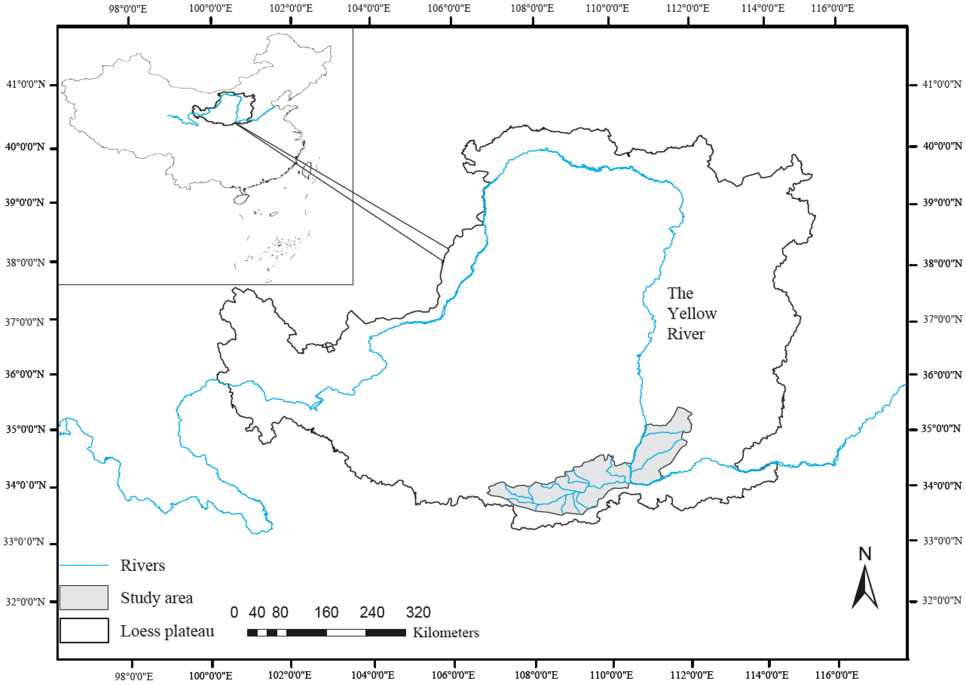
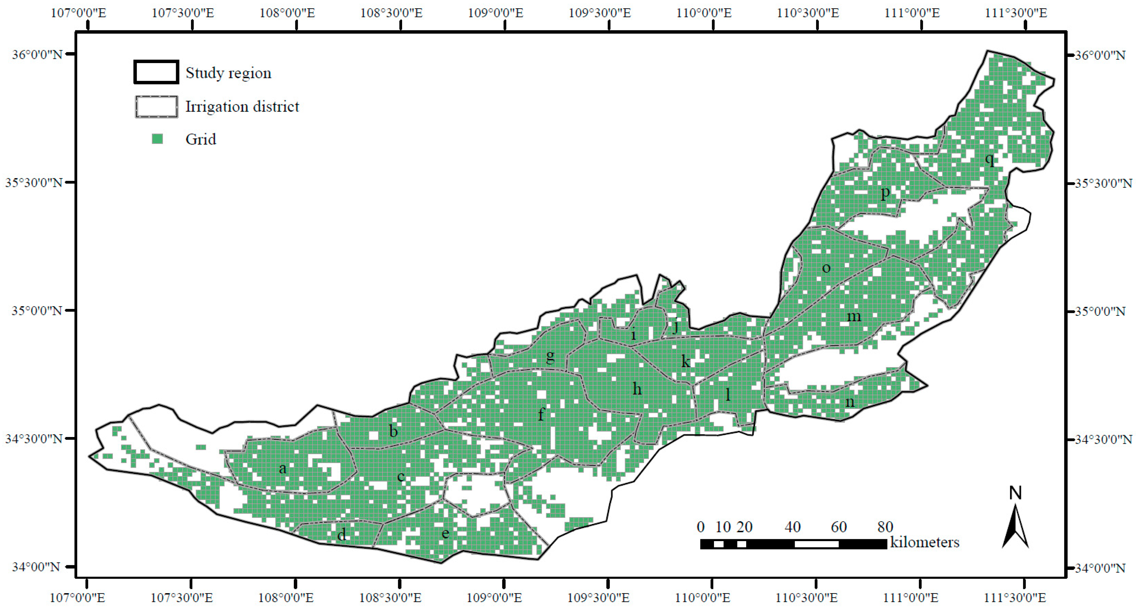
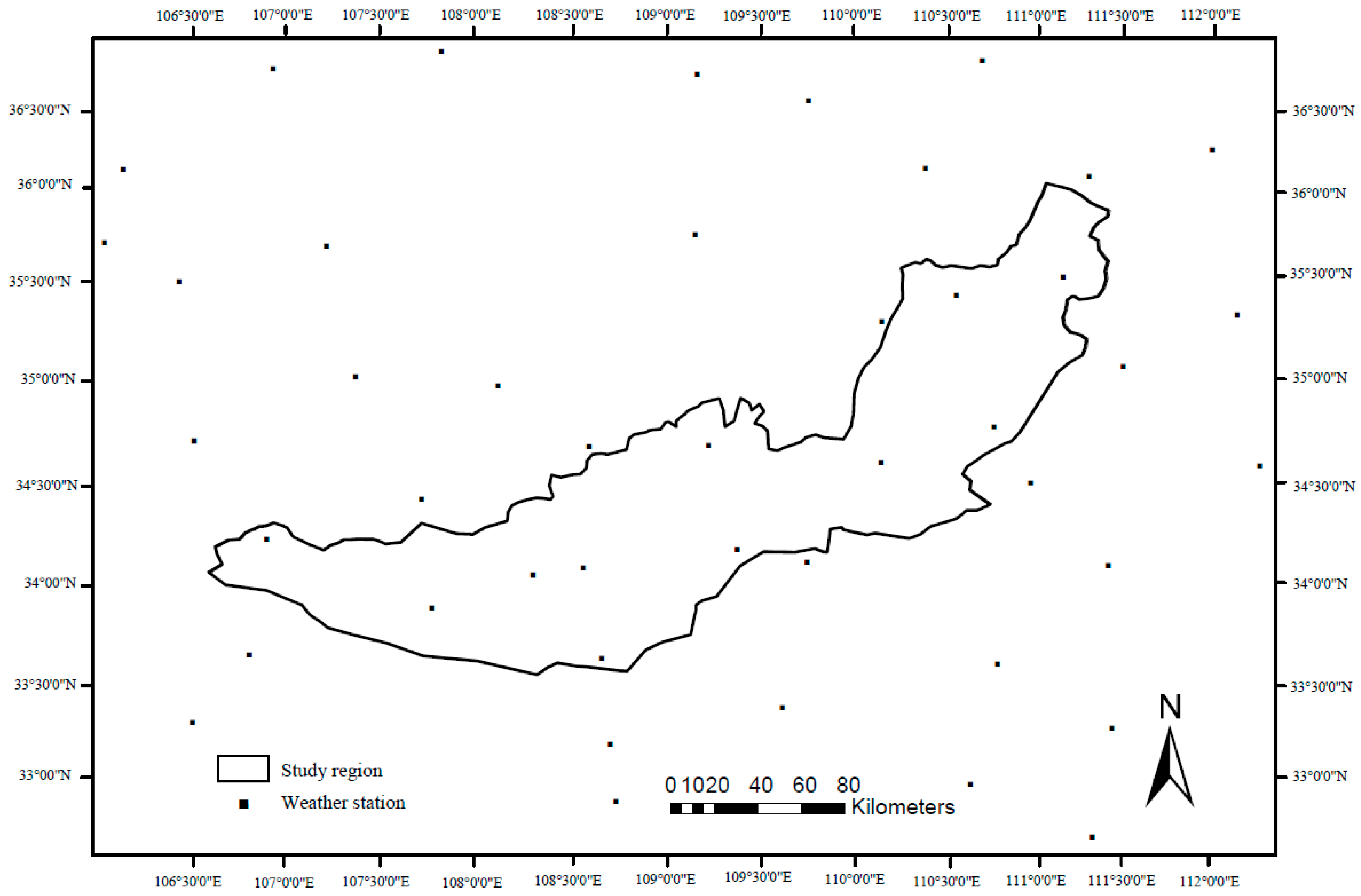
2.1. Study Region

The study region is the Fenwei Plain with an acreage of about 70,000 km² (34–36° N and 107°0′0″–111.30°0′48″ E). The plain is located in northern China and consumes more than 30% of the water amount of the Yellow River, which is the most important water resource in northern China (Figure 1). The climate of the region is semi-arid with a mean annual precipitation of 550 mm and temperature of 14.4 °C. The elevation of the region varies from 350 to 650 m. The agricultural production in the plain also contributes significantly to Chinese food security and highly depends on irrigation, but climate change already has had negative impacts on agriculture production, especially on agriculture water use of the plain [5]. Therefore, determining the impact of climate change on crop water requirements and the relevant driven factor are important to the development of regional and national agriculture.

2.2. Spatial and Temporal Analysis for Reference Evapotranspiration

2.2.1. Spatial and Temporal Scales

Compared to station data, interpolated gridded data provide regular and continuous spatial and temporal features allowing for studies of the spatial variability of climatic variables [20]. Gridded data are also of potential interest for high-precision simulations to provide more detailed results, but the computation time increases significantly with increasing spatial resolution [21]. To balance the spatial resolution and computation time, a 2×2 km grid resolution was applied in this study, and the spatial data of weather and land use were interpolated and resampled to this resolution. Considering that the results of this study can directly benefit the agricultural water management of the Fenwei Plain, the spatial distribution of the grids in the plain follow the distribution of agricultural land in the plain, which was collected by the Data Registration and Publication System for Resources and Environmental Sciences “www.resdc.cn/DOI/doiList.aspx (accessed on 30 January 2023)” and was mainly constructed from the satellite of Landsat 8 (Figure 2). The study region included 4811 grids after the resampling. The mean value of ET₀ and the climatic variables of the entire Fenwei Plain were calculated as the arithmetic mean of all grids in the study region.

Over 90% of the agriculture water amount was managed by 17 irrigation districts in the Fenwei Plain (Figure 3). The water management of these irrigation districts was usually planned on annual and seasonal time scales [8]. Since ET₀ is highly correlated with climatic variables, ET₀ also shows obvious seasonal variations similar to the changes in climatic variables [19,22]. Therefore, to consider the potential reference of the results for agriculture water use and agrometeorology, two temporal scales were analyzed in this study: annual and seasonal. The seasonal scale encompassed spring (March to May), summer (June to August), autumn (July to November) and winter (December to February), whereas the annual scale runs from January to December. Spatial analysis and computation were accomplished using ArcGIS 10.8 and MATLAB 2016a.

2.2.2. Calculation of Reference Evapotranspiration

ET₀ was calculated using the Penman–Monteith method with many meteorological variables, which showed wide applicability and high accuracy for estimating evapotranspiration [6]. The detailed equation is as follows (Allen, 1998):

$${ET}_0=\frac{0.408\Delta \left(R_n-G\right)+\gamma \left(e_s{-e}_a\right)u_2\left[900/(T_a+273)\right]}{\Delta +\gamma (1+0.34u_2)},$$

(1)

where R_n is the net radiation (MJ m⁻²d⁻¹), G is the soil heat flux (MJ m⁻²d⁻¹), T_a is the mean air temperature at 2 m height (°C), u₂ is the mean wind speed at 2 m height (m s⁻¹), e_s is the saturation vapor pressure (kPa), e_a is the actual vapor pressure (kPa), Δ is the slope of the saturation vapor pressure versus the air temperature curve (kPa °C⁻¹) and γ is the psychometric constant (kPa °C⁻¹).

The term (e_s − e_a) in Formula (1) is the vapor pressure deficit (VPD), which represents the dryness of the air and is one of the main drivers of vegetation evapotranspiration. VPD is a crucial variable used to understand how hydrology affects ecology and agriculture under climate change [23]. VPD was calculated from the maximum air temperature (T_max), minimum air temperature (T_min) and relative humidity (RH) as

$$VPD=\left(e_s-e_a\right)$$

(2)

$$e_s=\left[0.6108\times \exp \left(\frac{17.27\times T_{max}}{T_{max}+237.3}\right)+0.6108\times \exp \left(\frac{17.27\times T_{min}}{T_{min}+237.3}\right)\right]/2$$

(3)

$$e_a=\frac{RH}{100}\times e_s$$

(4)

Δ can be calculated by T_a. The specific calculation formula is as follows [1]:

$$\Delta =\frac{4098\times \left[0.6018\times \left(\frac{17.27\times T_a}{T_a+237.3}\right)\right]}{{(T_a+237.3)}^2}$$

(5)

γ can be calculated by air pressure (P). The calculation formula is as follows [1]:

$$\mathsf{\gamma }=0.665\times {10}^{-3}\times P$$

(6)

In summary, the terms in Equation (1) were transferred to or involved in five climatic variables including mean air temperature (T_a), wind speed (u₂), air pressure (P), vapor pressure deficit (VPD) and net radiation (R_n). These five variables were analyzed in the attribution analysis (Section 2.3) of changes in ET₀.

2.2.3. Historical and Future Climatic Data

This study involved monthly historical observed, historical simulated and future simulated climatic data. The historical observed variables of maximum, minimum and mean air temperature, wind speed, air pressure, relative humidity and duration of sunshine were collected from 45 national weather stations located in and around the study region to calculate observed ET₀ (Figure 3). The missing climatic data are generated using the linear interpolation method. Then, gridded historical observed data with a 2×2 km grid were interpolated using these weather station data and passed the generalized cross-validation. The software ANUSPLIN v4.4 was used for the interpolation, and the independent variables were longitude and latitude, with elevation as the covariate. More interpolation details are showed in [5]. The data of 31 years from 1985 to 2015 were collected as the historical period (baseline period).

The historical and future simulated climatic data were collected among the global climate models (GCM) in CMIP6 “https://esgf-data.dkrz.de/search/cmip6-dkrz/ (accessed on 30 January 2023)”. The periods from 1985 to 2015 and from 2030 to 2060 were defined as the baseline period and future period, respectively. The simulated monthly climatic data of maximum, minimum and mean air temperature, wind speed, air pressure, relative humidity and solar radiation were collected from the GCM models to calculate the simulated ET₀. For better simulation of ET₀, the net radiation term R_n in Formula (1) was calculated as follows [24]:

$$R_{n\_CMIP6}=\left(rsds-rsus\right)-(rlus-rlds),$$

(7)

where R_{n_CMIP6} is the net radiation calculated by the data from CMIP6, and rsds, rsus, rlus and rlds are surface downwelling shortwave radiation, surface upwelling shortwave radiation, surface upwelling longwave radiation and surface downwelling longwave radiation, respectively.

As mentioned before, the accuracy of CMIP6 has been further improved compared with previous projects, for example, the resolution of some GCM models has reduced to 100 km. Therefore, to meet more accurate and detailed needs for water management and to reduce the downscaling uncertainty, the GCM models possessing the same monthly scale, variant label (r1i1p1f1), nominal resolution (100 km) and variables (the given climatic variables) were selected from CMIP6. Thus, four GCM models (MPI-ESM1-2-HR, MRI-ESM2-0, CMCC-ESM2 and CAS-ESM2-0) were selected. Then, four sets of the simulated climatic variables were calculated to obtain four sets of the simulated ET₀ after the downscaling and bias correction for the climatic variables (see the next Section 2.2.4). The method of multi-model ensemble mean (MME) has shown better simulation performance than individual GCM in many studies [25]. So, the ensemble prediction of simulated ET₀ was used in this study using the MME with equal weighing, which was calculated by the arithmetic mean value of the four sets of simulated ET₀.

At the current rate of adoption of climate change mitigation measures, global mean temperature is projected to rise by 3.2 °C in 2100 [26]. Therefore, we chose the middle forcing scenario SSP245 and high forcing scenario SSP585 in this study, which implies a radiative forcing in 2100 of 4.5 W m⁻² and 8.5 W m⁻² with a global mean temperature rise of about 3 °C and 5 °C, respectively [19].

2.2.4. Downscaling Process and Bias Correction

The output of GCMs is normally large-scale data with the resolution ranging from 100 km to 500 km and needs downscaling for application at regional scale [19]. Downscaling includes two steps: temporal downscaling and spatial downscaling. Since this study involved seasonal and annual scales, monthly data were selected from the CMIP6 without further temporal downscaling. Regarding spatial downscaling, the method of inverse distance-weighted interpolation was used, which has shown satisfactory interpolation performance in many downscaling studies [27]. The spatial resolution of simulated climatic data after downscaling is 2 × 2 km.

The simulated climatic variables from the GCMs need bias correction through comparison with the observed climatic variables before the data can be used in further applications [16]. The bias correction process in this study included creating a q–q function to calibrate the bias between the observed and simulated data, which were collected from the same period of 1965 to 1994, and then using the data from the period of 1995 to 2015 to validate this correction function [28]. Eventually, the simulated climatic data in the future period were corrected by this function. In consideration of the gridded simulation in this study, the q–q function was created for each grid.

The performance of downscaling and bias correction was evaluated by the correlation coefficient (R²) and the root mean square error (RMSE), which were calculated as

$$R^2={\left[\frac{\sum \left(S_i-\overline{S}\right)\left(O_i-\overline{O}\right)}{\sqrt{\sum {\left(S_i-\overline{S}\right)}^2{\left(O_i-\overline{O}\right)}^2}}\right]}^2,$$

(8)

where $O_i$ and $S_i$ are the observed and simulated climatic variables, respectively. $\overline{O}$ and $\overline{S}$ are mean values of the observed and simulated data, respectively. $R^2$ close to 1 indicates a favorable agreement between the observed and simulated climatic variables.

$$RMSE=\sqrt{\sum {\left(O_i-S_i\right)}^2/n},$$

(9)

where n is the number of observed data. RMSE close to 0 indicates a small deviation between the observed and simulated climatic variables.

2.2.5. Trend Detection

Detecting the change trend of climatic variables is an essential step in the research on the impact of climate change. A non-parametric Mann–Kendall method (MMK) was used for the trend detection, which has shown satisfactory performance in the studies of long-term trend analysis [29]. The Z statistic in MMK follows the standard normal distribution with a mean of variance of one under the null hypothesis of no trend in the detected series. The significant level is 0.05 in this study, and the trend in the series is significant when |Z| ≥ 1.96 [16]. Positive and negative values of Z indicate an increased and decreased tendency, respectively. The ET₀ trend in each grid was detected by the MMK.

2.3. Methods of Attribution Analysis

2.3.1. Sensitivity Index

The sensitivity index has been frequently used for studying the impact of climatic variable changes on evapotranspiration changes [30]. In the calculation of the sensitivity index, the ET₀ changes are dimensionless by using the partial derivative for calculation simplicity. The specific calculation is as follows [31]:

$${SI}_x=\underset{\Delta x\to 0}{\lim }\left(\frac{\Delta E{T}_0/E{T}_0}{\Delta x/x}\right)=\frac{\partial E{T}_0}{\partial x}·\frac{x}{E{T}_0},$$

(10)

where SI_x is the sensitivity index of a climatic variable regarding ET₀ changes and x is the value of the climatic variable. The sensitive degrees are divided by the absolute value of S_x: |SI_x| ≤ 0.05 indicates no sensitivity, 0.05 ≤ |SI_x| ≤ 0.2 indicates moderate sensitivity, 0.2 ≤ |SI_x| ≤ 1.0 indicates high sensitivity and |SI_x| ≥ 1.0 indicates extreme sensitivity [32]. The calculation of SI_x was accomplished using MATLAB 2016a.

2.3.2. Contribution Rate

A previous study has pointed out that using the sensitivity index alone cannot comprehensively analyze the impact of climatic variables on ET₀ changes [31]. Thus, a contribution rate of climatic variables impacting ET₀ was defined based on the sensitivity index as [31]:

$${Con}_x={SI}_x·{RC}_x$$

(11)

$${RC}_x=\frac{n·B_x}{\left|M_x\right|}·100\%,$$

(12)

where Con_x is the contribution rate of a climatic variable regarding ET₀ changes, SI_x is the sensitivity index of the climatic variable, RC_x is the relative changes of the climatic variable over the studied period, n is years in the time period of the study, i.e., 31 years in this study, M_x is the mean value of the climatic variable in the n years and B_x is the annual (or seasonal) linear rate (least square method) of the climatic variable over the n years. Negative and positive contribution rates indicate that changes of the climatic variable cause an increase and decrease in ET₀, respectively. The larger the absolute value of Con_x, the greater impact of climatic variable changes on the ET₀ change. The climatic variable with the largest absolute value of Con_x is the dominant factor for ET₀ change. The actual change rate of ET₀ over n years was calculated by Equation (12) and indicated as RC_ET0.

The relative change rate of ET₀ is the sum of the contribution rate of each climatic variable, and the specific calculation was as follows:

$${Con}_{{ET}_0}={Con}_{VPD}+{Con}_{Ta}+{Con}_{WS}+{Con}_{R_n}+{Con}_P,$$

(13)

where Con_ET0 is the relative change rate of ET₀ caused by the combined effect of the five climatic variables, and Con_VPD, Con_Ta, Con_u2, Con_Rn and Con_P are, respectively, the contribution rate of VPD, T_a, u₂, R_n and P regarding change in ET₀.

3. Results

3.1. Evaluation of Bias Correction

The performance of the four GCMs in simulating the five climatic variables and ET₀ were all improved after downscaling and bias correction (

Table 1. Simulation performance of the climatic variables and reference evapotranspiration after downscaling and bias correction.

GCM Models		Air Temperature (°C)		Air Pressure (k Pa)		Wind Speed (m s−1)		Solar Radiation (W m−2)		Vapor Pressure Deficit (k Pa)		ET0 (mm)
		R2	RMSE	R2	RMSE	R2	RMSE	R2	RMSE	R2	RMSE	R2	RMSE
MPI-ESM1-2-HR	Calibration	71.2%	0.87	83.2%	2.56	56.9%	0.93	53.6%	0.77	74.1%	0.11	55.1%	30.9
	Validation	81.9%	0.83	85.7%	1.15	68.7%	0.91	61.8%	0.67	81.5%	0.09	68.3%	26.2
MRI-ESM2-0	Calibration	80.9%	1.44	96.3%	3.61	62.6%	1.71	62.5%	0.81	77.9%	0.12	79.4%	18.1
	Validation	92.7%	0.64	98.5%	1.67	76.2%	1.23	69.1%	0.62	82.8%	0.1	88.1%	14.1
CMCC-ESM2	Calibration	79.1%	2.99	80.5%	4.33	55.7%	1.96	73.9%	0.52	72.3%	0.16	65.3%	31.3
	Validation	90.2%	2.1	85.2%	2.62	69.1%	1.44	79.2%	0.43	79.3%	0.13	76.7%	27.5
CAS-ESM2-0	Calibration	87.3%	1.94	90.7%	5.79	50.6%	1.55	69.5%	0.23	81.9%	0.19	76.6%	26.3
	Validation	95.2%	1.23	93.9%	3.98	64.9%	1.26	76.8%	0.2	86.2%	0.16	85.2%	22.9
Ensemble	Calibration											78.9%	17.7
	Validation											89.5%	13.9

). The R² and RMSE of the variables and ET₀ in validation were all, respectively, increased and decreased compared to the values in calibration. Similarly, the ranges of R² and RMSE of the variables and ET₀ were narrowed after the correction. The simulation performance of air temperature and pressure were better than other climatic variables, demonstrated by lower RMSE and higher R² ranging from 81.9% to 98.5%. The R² and RMSE of the ensemble-simulated ET₀ were both, respectively, higher and smaller than the values of the individual GCM.

3.2. Trend Detection and Changes of ET₀ under Climate Change

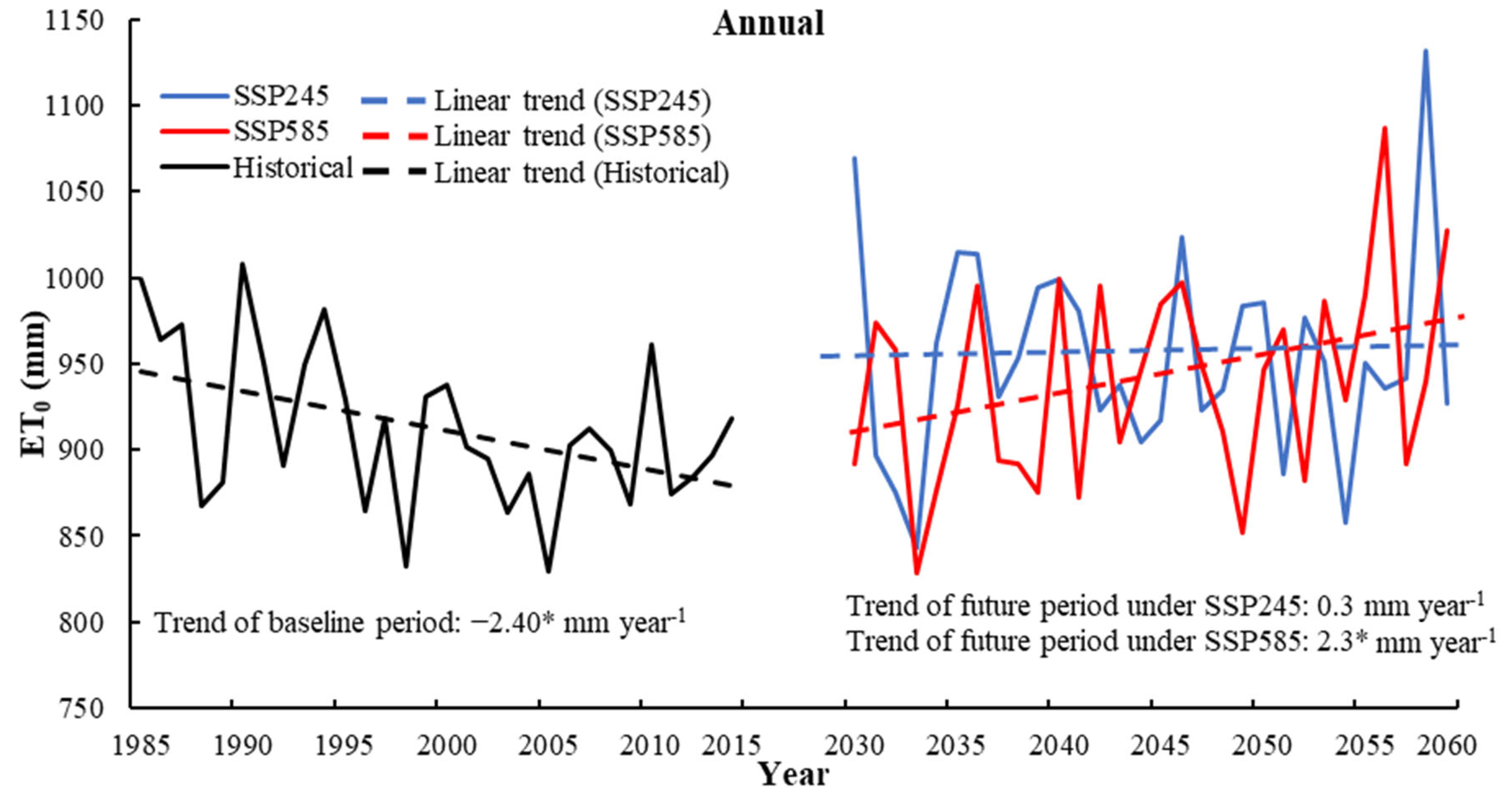
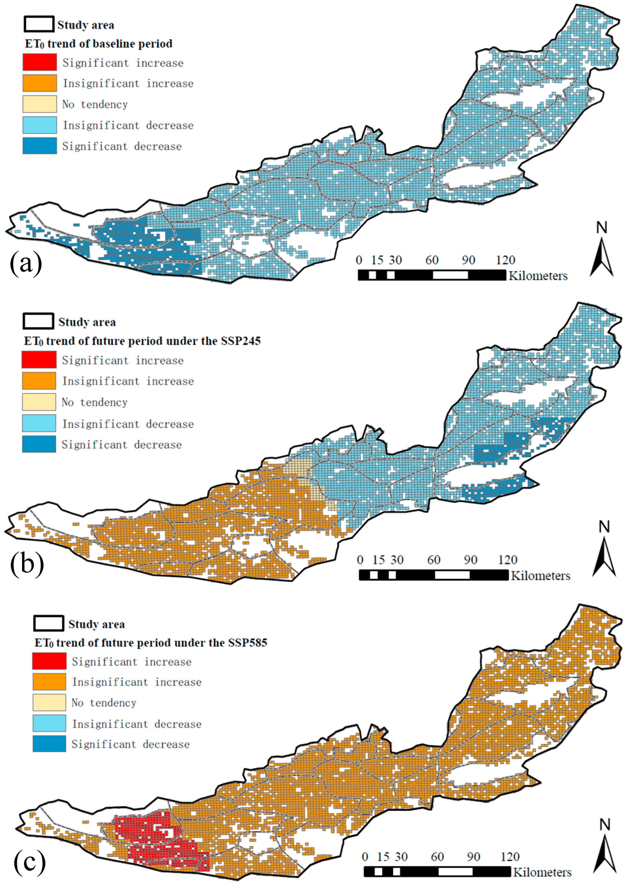
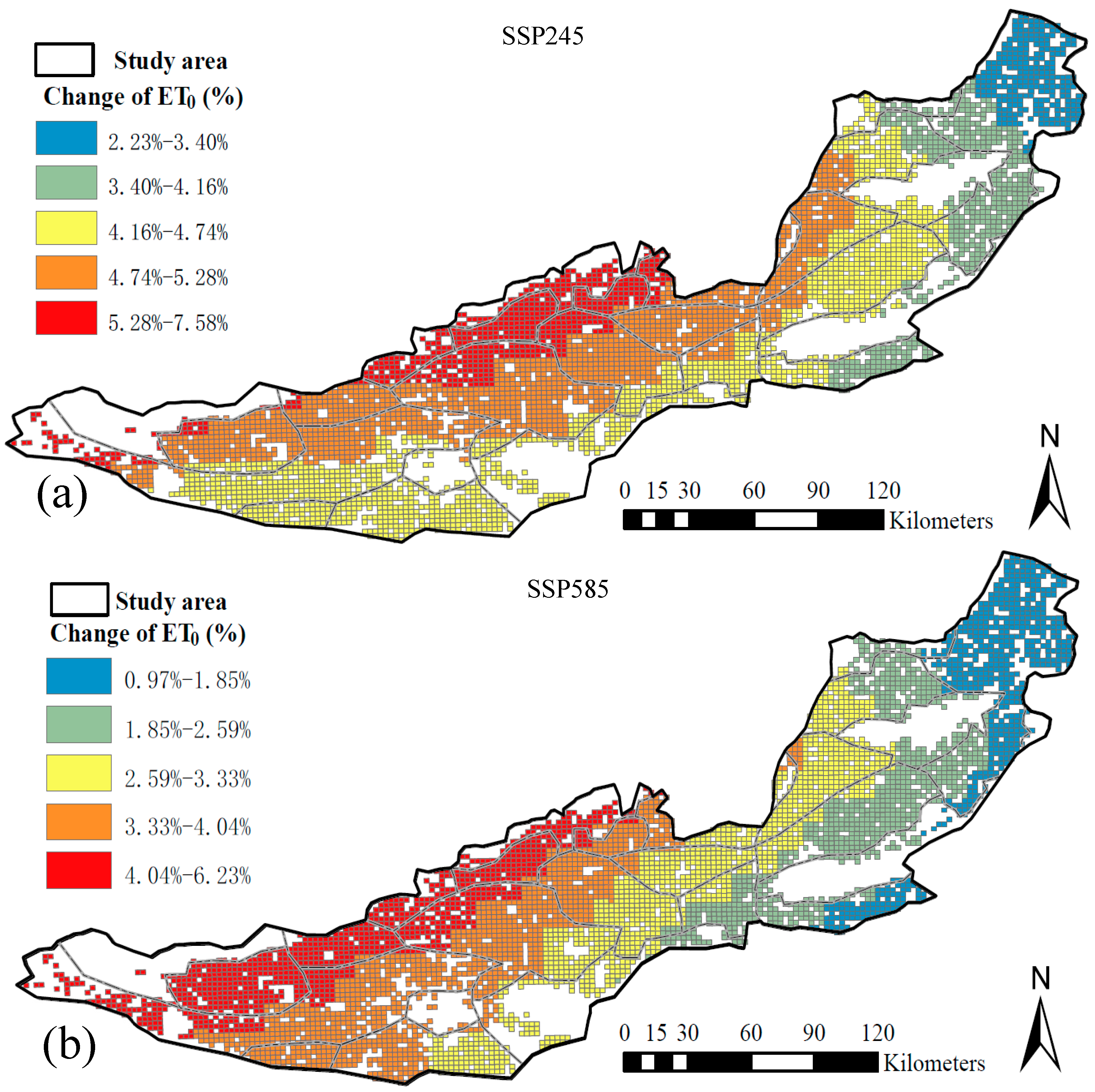
3.2.1. Trend Detection and Relative Changes of ET₀ at Annual Scale

The mean annual ET₀ of the entire Fenwei Plain showed a significant decreasing trend in the baseline period from 1985 to 2015 with a rate of −2.4 mm per year (Figure 4). In the future period from 2030 to 2060, the annual ET₀ showed an insignificant increasing trend under the SSP245 scenario. Under the SSP585 scenario with higher radiative forcing and temperature compared to the SSP245 scenario, the annual ET₀ showed a significant increasing trend at a rate of 2.3 mm per year.

In the future period, the mean annual ET₀ of the entire Fenwei Plain is 954 mm and 939 mm under the SSP245 and SSP585 scenarios, respectively, which increases 4.6% and 3.0%, respectively, compared to 912 mm in the baseline period.

The annual ET₀ of all grids in the Fenwei Plain showed significant and insignificant decreasing trends in the baseline period (Figure 5a). In the future period under the SSP245 scenario, about half of the grids in the Fenwei Plain showed significant and insignificant decreasing trends, and these grids were mostly located in the eastern area of the plain. Accordingly, about half of the grids in the Fenwei Plain showed insignificant increasing trend, and these grids were mostly located in the western area of the plain (Figure 5b). In the future period under the SSP585 scenario, all grids showed significant and insignificant increasing trends (Figure 5c).

The annual ET₀ changes between the future period relative to the baseline period were calculated as the difference between the mean annual ET₀ of the future and baseline period (Figure 6). The ET₀ of all grids showed varying increases in the future period. The ET₀ under the SSP245 scenario increased from 2.2% to 7.6% compared to the baseline period. The ET₀ under the SSP585 scenario increased from 1.0% to 6.2% compared to the baseline period. The increases in ET₀ become greater from the eastern to western areas of the Fenwei Plain under both the SSP245 and SSP585 scenarios.

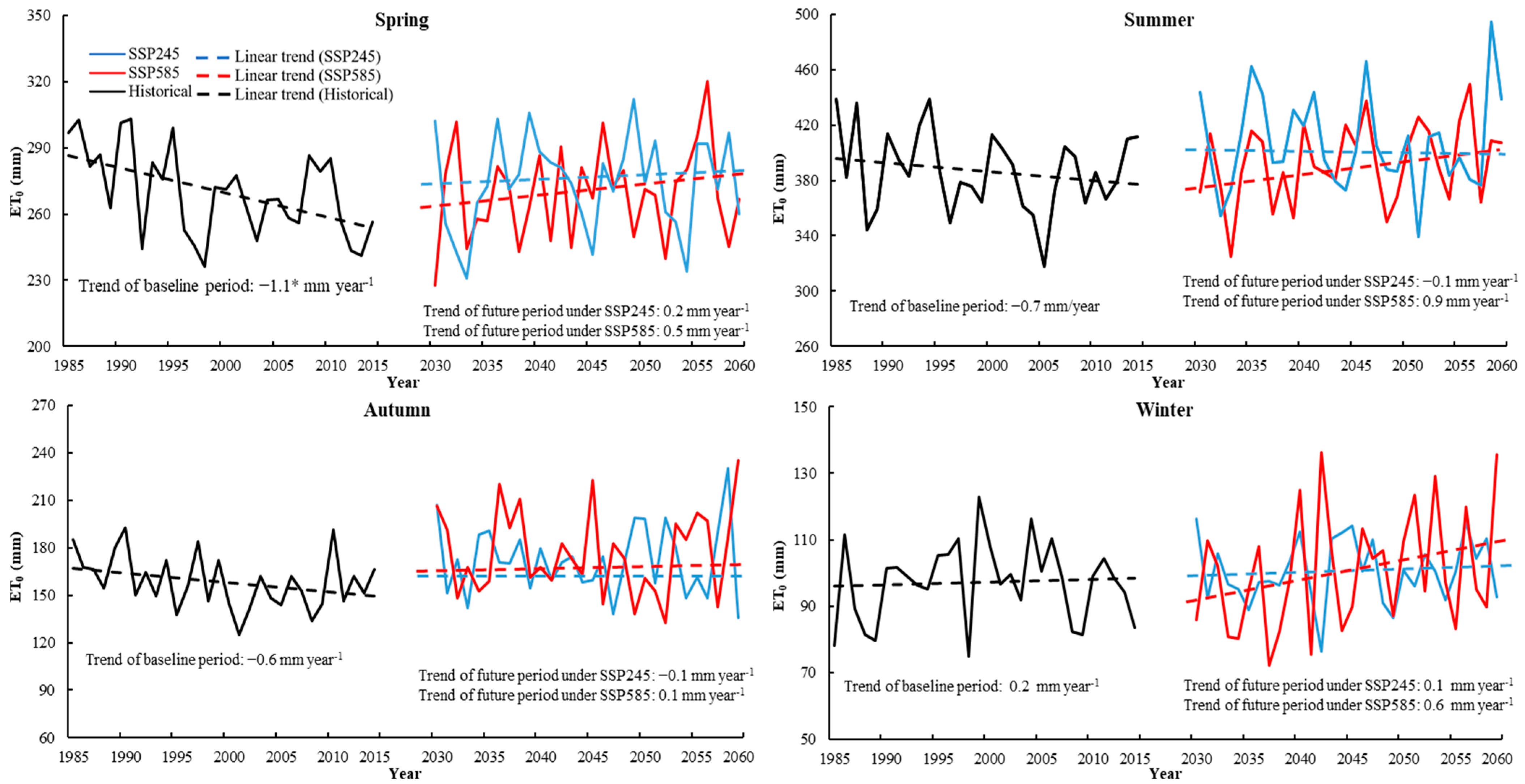
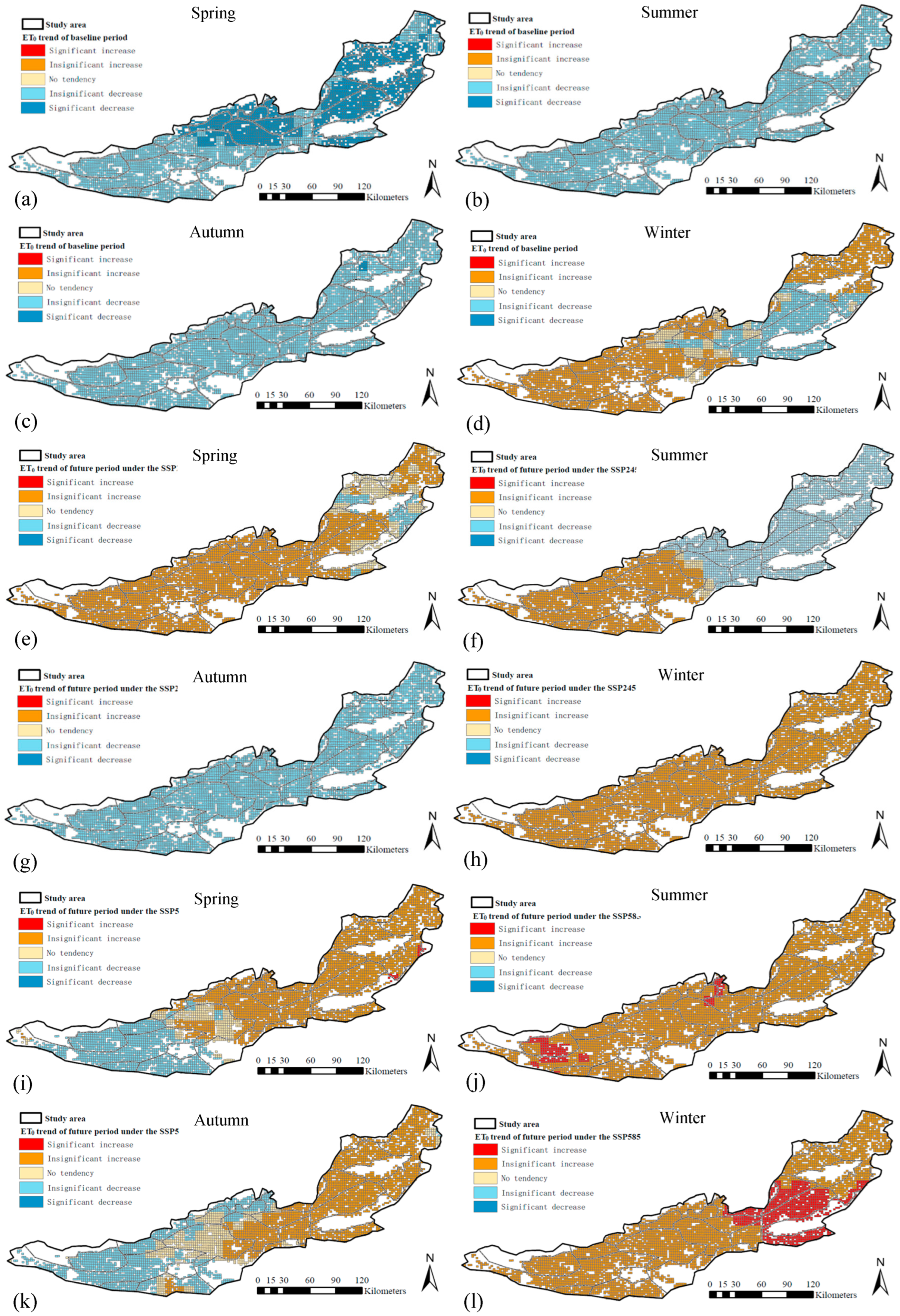
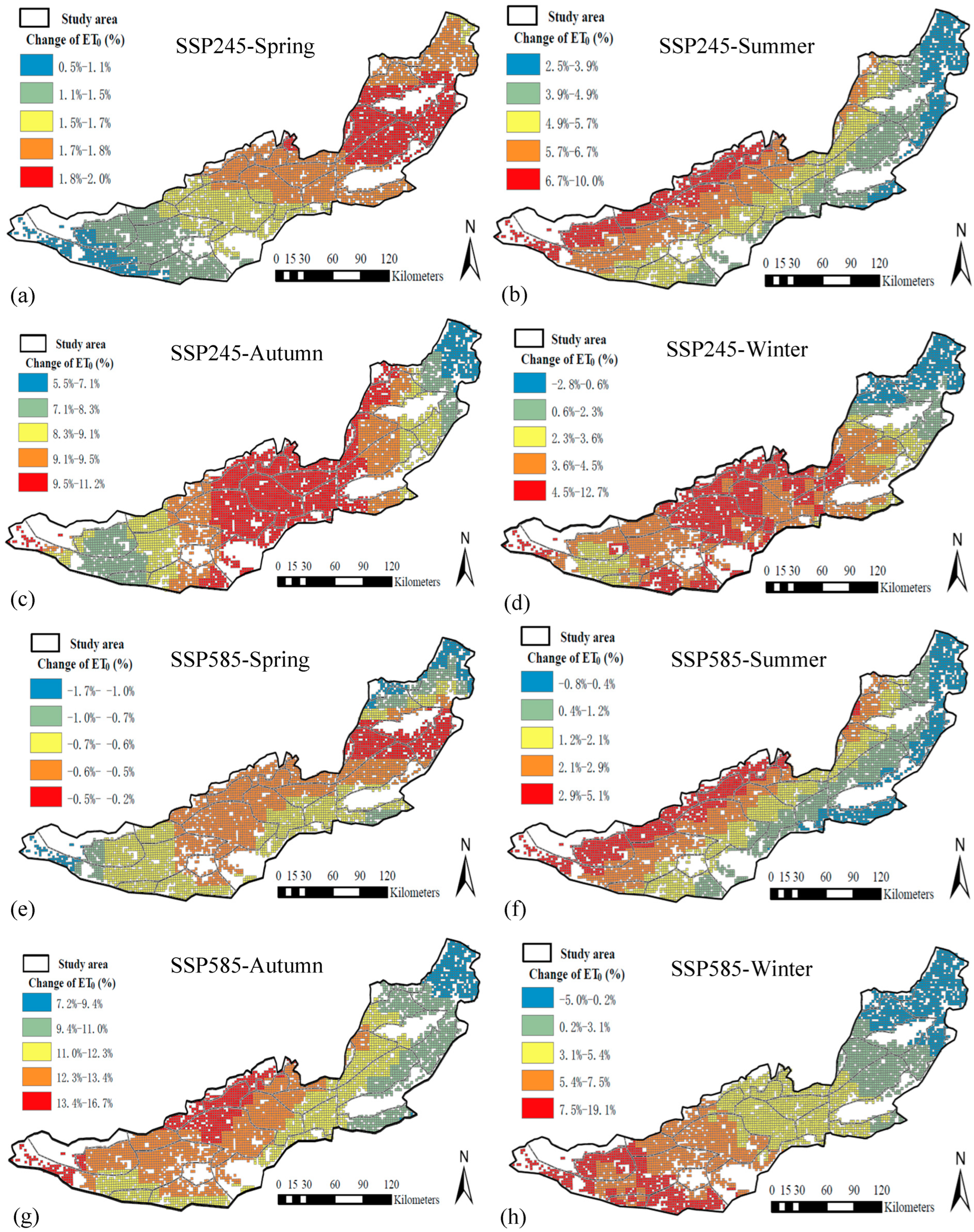
3.2.2. Trend Detection and Relative Changes of ET₀ at Seasonal Scale

The ET₀ in the four seasons showed different change trends (Figure 7). In the baseline period from 1985 to 2015, the ET₀ showed a significant decreasing trend in spring with a decrease rate of 1.1 mm per year. The ET₀ in summer and autumn both showed insignificant decreasing trends. The ET₀ in winter showed a slight insignificant increasing trend. In the future period from 2030 to 2060, the ET₀ in the four seasons showed slight insignificant decreasing or increasing trends under the SSP245 scenario, and the ET₀ in the four seasons all showed insignificant increasing trends under the SSP585 scenario.

Compared to the baseline period, the mean ET₀ of the entire Fenwei Plain increased in all four seasons under the SSP245 scenario, with autumn showing the largest increase of 8.6% (

Table 2. Changes in seasonal mean ET₀ (mm) of the entire Fenwei Plain under the SSP245 and SSP585 scenarios for the future period relative to the baseline period.

Seasons	ET0 in the Baseline Period	ET0 under the SSP245 Scenario	The SSP245 Scenario Relative to the Baseline Period	ET0 under the SSP585 Scenario	The SSP585 Scenario Relative to the Baseline Period
Spring	270.1	274.5	1.6%	269.3	−0.3%
Summer	386.6	407.0	5.3%	393.1	1.7%
Autumn	158.4	172.1	8.6%	176.7	11.6%
Winter	97.3	100.5	3.3%	101.0	3.9%

Note: ‘The SSP245/585 scenario relative to the baseline period’ indicates the ET₀ changes under the SSP245/SSP585 scenarios relative to the baseline period.

). Under the SSP585 scenario, the ET₀ in summer, autumn and winter increased, and autumn showed the largest increase of 11.6%. The mean ET₀ in spring showed a slight decrease of 0.3% under the SSP585 scenario relative to the baseline period.

All grids for the plain in the baseline period showed insignificant or significant decreasing trends in spring, summer and autumn, and the number of the grids showing significant decreasing trends was highest in spring (Figure 8a–c). Part of the grids in the plain showed an insignificant increasing trend in winter (Figure 8d). Under the SSP245 scenario, the grids showed slight insignificant decreasing, increasing or no trends (Figure 8e–h). Under the SSP585, all the grids showed significant and insignificant increasing trends in summer and winter (Figure 8j,l), and the grids showed slight insignificant decreasing, increasing or no trends in spring and autumn (Figure 8i,k).

The ET₀ of all grids in the Fenwei Plain showed varying increases in spring, summer and autumn under the SSP245 scenario relative to the baseline period, with an increase in autumn ranging from 5.5% to 11.2%, thereby being higher than for other seasons (Figure 9a–c). In the winter under the SSP245 scenario, the ET₀ increased for most of the grids and decreased for a few (Figure 9d). Under the SSP585 scenario, the ET₀ increased for all grids in autumn (Figure 9c), and ET₀ increased for most of the grids and decreased for the other grids in spring, summer and winter (Figure 9e,f,h).

3.3. Attribution Analysis of Climatic Variables to ET₀ Change

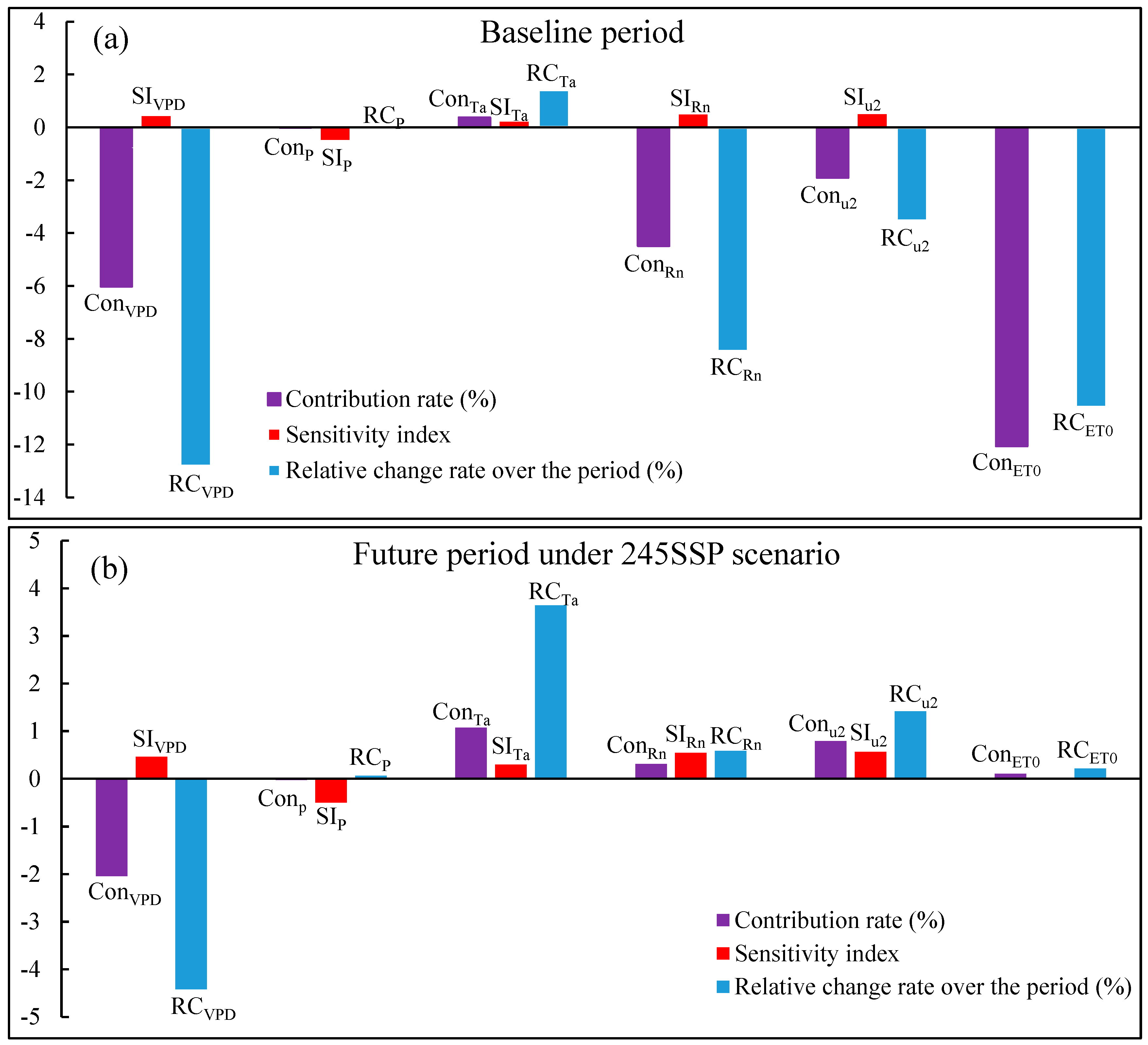
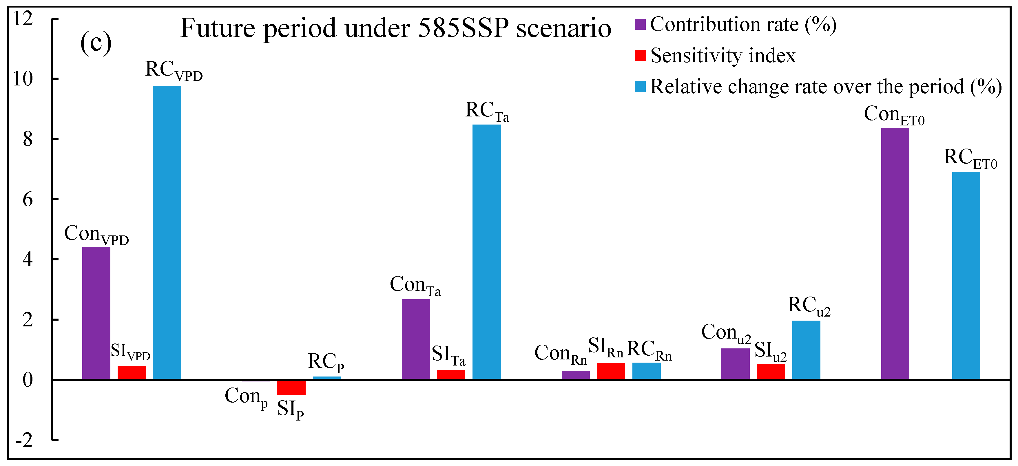
3.3.1. Attribution Analysis at Annual Scale

In the baseline period, VPD was the largest contribution factor with a contribution rate of −6.0% to the decrease in ET₀ (Figure 10). The contribution rate is the product of the sensitivity index (SI) and relative change rate (RC) over the period (Equation (11)), and the RC of VPD showed the largest decrease of 12.8%, which was the main reason why VPD showed the largest contribution. Meanwhile, the VPD did not achieve the highest SI, i.e., VPD was not the most sensitive climatic variable to ET0 change. The R_n was the second largest contribution and sensitive factor to ET₀ change in the baseline period. For those climatic variables having a larger contribution rate in the baseline period (Figure 10a), such as VPD, R_n and u₂, the absolute values of RC were far higher than the absolute values of SI.

In the future period, VPD also showed the largest contribution rates with −2.0% and 4.4% to ET₀ change under the SSP245 and SSP585 scenarios, respectively. Like for the baseline period, VPD showed the largest decrease rate over the period under the SSP245 and SSP585 scenarios but was not the most sensitive climatic variable to ET₀ change. T_a was the second largest contribution factor to ET₀ change in the future period under the SSP245 and SSP585 scenarios. Like for the baseline period, the absolute values of RC of those variables having larger contributions were far higher than the absolute values of SI of the variables in the future period, such as VPD, T_a and u₂ (Figure 10b,c).

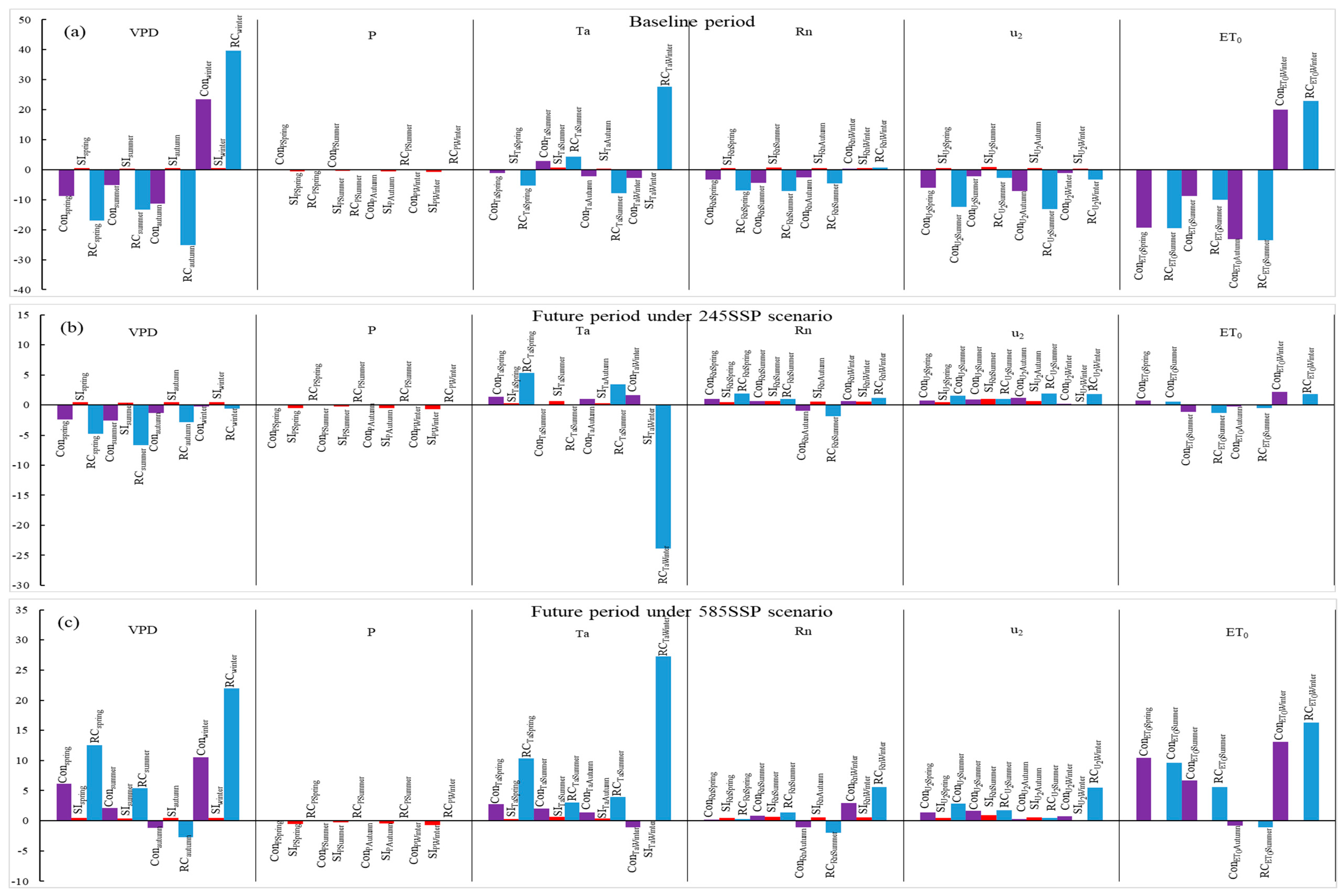
3.3.2. Attribution Analysis at Seasonal Scale

In the baseline period, VPD showed the largest contribution to ET₀ change in all four seasons (Figure 11a), as was the case at the annual scale. The large RC was the main reason for the contribution of VPD to ET₀ change, while the second largest contribution to ET₀ change differed in the four seasons; u₂ was the second contribution factor in spring and autumn, R_n was the second contribution factor in summer and T_a was the second contribution factor in winter.

In the future period under the SSP245 scenario, VPD showed the largest contribution to ET₀ change in spring, summer and autumn, and T_a showed the largest contribution to ET₀ change in winter (Figure 11b). T_a had the second largest contribution in spring, u₂ had the second largest contribution in summer and autumn and R_n had the second largest contribution in winter. The largest RC of VPD in spring and summer and the largest RC of T_a in winter caused the corresponding climatic variables to be the greatest contribution factors to ET₀ change. In the future period under the SSP585, VPD still showed the largest contribution to ET₀ change in spring, summer and winter, and T_a showed the largest contribution to ET₀ change in autumn (Figure 11c). T_a had the second largest contribution in spring and summer, and VPD had the second largest contribution in autumn. Similarly, the largest RC of VPD in spring and summer and the largest RC of T_a in autumn are still the reason for the corresponding climatic variables being the largest contribution factors to ET₀ change. Like at the annual scale, the absolute values of RC of the most contribution factors at the seasonal scale are far higher than the absolute values of SI of those factors.

There was little difference between Con_ET0 and RC_ET0 at both the annual and seasonal scale, which indicates that the relative changes of ET₀ caused by the five climatic variables are very close to the actual changes of ET₀.

4. Discussion

4.1. The Simulation Performance of the GCM Models

The simulation performance of the GCM models was improved after downscaling and bias correction, and the simulated ensemble ET₀ showed better simulation performance than the performance of the individual GCM. The simulation performance of air temperature and pressure were better than other climatic variables, which may be explained by the greater stability of air pressure relative to the other variables and the focus on simulation of temperature in the development of the GCM models [33]; similar results have been reported in studies simulating with the GCM models [34]. The temperature varies from day to day, and this variation is not reflected in the monthly temperature used here [35]. Since there is a non-linear relationship between vapor pressure and temperature, our use of monthly temperatures to calculate the VPD would lead to a slight underestimation compared with using daily values. This is reflected in slightly lower ET₀ estimates. However, the same procedure was used across the entire study; thus, it does not affect conclusions of ET₀ trends and attribution analysis.

4.2. The Trend and Changes of ET₀ at Annual Scale

Evapotranspiration is expected to increase with increasing temperature under climate change. However, some actual and simulated data have shown a decreasing trend in ET₀ (evaporation paradox) during the 1950s to 2010s [36,37]. Our study showed a significant decreasing trend in annual ET₀ in the Fenwei Plain during the baseline period from 1985 to 2015 (Figure 4). The attribution analysis indicates the large RC of VPD and R_n are the two main reasons for the ET₀ decrease in the baseline period. Huang et al. [38] and Yuan et al. [33] reported similar results of decreased VPD and R_n during the 1980s to 2010s in northern China. Du et al. [12] detected no significant trend in ET₀ for the entire Loess Plateau (which covers the Fenwei Plain) during 1974–2019, which indicates that different spatial scales lead to different analytical results, and different research subjects need to be studied with their appropriate scales [21].

In the future period from 2030 to 2060, the trend in annual ET₀ turned to an increasing trend. Specifically, the annual ET₀ under the SSP245 and SSP585 scenarios showed insignificant and significant increasing trends, respectively. The attribution analysis indicates that the large RC of VPD and T_a are the main reasons for the ET₀ increase. The VPD showed opposite change trends between the baseline and future period, which could be explained by the fact that an abrupt increasing VPD was detected in the late 2000s in northwest China, and this change may have been caused by increasing temperature and decreasing actual vapor pressure [23,39]. Temperature replaced R_n as the second largest contribution factor in the future period, partly because the relative change amplitude of temperature in the future period is larger than the other variables in the projected data of CMIP6 [19]. The results showed that the annual ET₀ of the Fenwei Plain in the future period is higher than the ET₀ in the baseline period, which is consistent with the increasing trend in the future period relative to the decreasing trend in the baseline period. The mean annual ET₀ under the SSP245 scenario is slightly higher than the ET₀ under the SSP585 despite the ET₀ showing a significant increasing trend under the SSP585 and an insignificant increasing trend under the SSP245, respectively. This indicates that the mean value over the period cannot directly represent the change trend over the period; the existence of fluctuation in climatic variables and the impact of climate change on ET₀ is nonlinear and complex [40]. The spatial variation of the annual ET₀ change and trend in the Fenwei Plain is mainly reflected in the differences between the eastern and western area of the plain.

4.3. The Trend and Changes of ET₀ at Seasonal Scale

The ET₀ trends of spring, summer and autumn in the baseline and future periods were roughly in accordance with the ET₀ trend at the annual scale in the corresponding periods. However, the winter ET₀ showed a continuous increasing trend in both the baseline and future period even though the annual ET₀ showed an opposite trend from the baseline period to the future period (Figure 4 and Figure 7). Feng et al. [41] reported a significant increasing trend in ET₀ for winter in northern China, which is similar to this study. The ET₀ change and trend between the four seasons showed obvious differences since the relevant climatic variables show distinctly different seasonal characteristics of change and trend [42].

The contribution ranks for the four seasons differed and they further changed from the baseline period to the future period, although VPD was the major contribution factor to ET₀ change in both periods. Like for the annual scale, the contribution of T_a increased from the baseline period to the future period, which could be caused by the greater relative change in air temperature in the future. The large RCs of seasonal climatic variables were still the main reasons for ET₀ change. The results at annual and seasonal scales both indicate that the major contribution factors are mostly the climatic variables with large RCs (relative changes over the period) instead of the most sensitive variables for affecting change in ET₀, which demonstrates that SI can quantify the impact extent of climatic variable changes on ET₀ change but cannot fully determine the actual contribution of changes in the variables to ET₀ changes, because ET₀ change is not only determined by the sensitivity of the variables, but is also related to the actual changes in the variables.

Like the results at the annual scale, the spatial differences of the seasonal ET₀ change and trend are also mainly reflected in the differences between the eastern and western area of the Fenwei Plain. Due to the impact of the mountains surrounding the Fenwei Plain, the eastern area of the plain showed a higher temperature and drier climate compared to the western area of the plain [43], so these regional climate differences may be the reason for the spatial differences of ET₀ change in the plain.

4.4. Impaction and Adaptation Prospects of Agriculture Water Use and Crop Cultivation

The increasing ET₀ would lead to a significant increase in crop evapotranspiration [1], but would not directly lead to a significant increase in crop yield. The results in this study showed an increasing annual ET₀ in the Fenwei Plain under the two future scenarios. Therefore, improving the efficiency of crop water use is a crucial adaptation under climate change for the plain with constraints on the water resources. Adapting the irrigation schedule is another important adaptation for the impact of climate change on agriculture water use [4]. The crop evapotranspiration in summer and autumn will increase more in the future (Table 2), which indicates the crops that critical periods of water requirement are in summer and autumn need to increase irrigation, such as for the spring and summer maize, apple and kiwi fruit cultivated in the plain. Similarly, more water needs to be allocated in summer and autumn for the water management of the irrigation district. The irrigation in winter also needs to increase appropriately for the crops that have critical periods of water requirement in the winter, such as increasing irrigation in the seedling stage of winter wheat. In addition, with the decreasing ET0 of spring under the SSP585 scenario, allocating the water amount of spring to another season moderately is also a fair adaptation.

A shorter time scale (e.g., daily scale) is more conducive to agricultural practices, but this also implies a huge computing time. With the improvement of computer performance, future studies with shorter time scales should be conducted.

The differences in ET₀ change between the eastern and western area of the Fenwei Plain indicate that the western area of the plain will need more water in annual water allocation to satisfy the relative higher crop evapotranspiration in the future (Figure 5 and Figure 6). Using the established aqueducts between irrigation districts could balance the water requirement differences between the eastern and western area of the plain in the future. Improving crop water use efficiency and increasing irrigation may not be sufficient to address the impact of climate change in conditions with limited water resources like the Fenwei Plain [5]. The adjustment of cropping systems is also a fair adaptation in agronomy. Based on the results of this study, we suggest enlarging the area of crops with lower water requirement in the western area of the plain and reducing the area of crops with higher water requirements in the eastern area, such as, enlarging the planting area of summer maize and jujube in the corresponding area and reducing the planting area of winter wheat and spring maize appropriately in the corresponding area. The adaptations under the two scenarios also need to be differentiated, for instance, the irrigation districts g, i and j require increasing irrigation under the SSP245 scenario, but the irrigation districts a, b and g require increasing irrigation under the SSP585 scenario (Figure 6). At the seasonal scale, the adaptation need to be various due to the different change and trend in ET₀ between the seasons, for instance, the increasing irrigation needs to be allocated more in the eastern area of the plain in winter under the SSP585 scenario, and the increasing irrigation needs to allocated more in the middle area of the plain in winter under the SSP245 scenario (Figure 9).

VPD showed a large contribution to ET₀ change, and VPD also affected vegetation transpiration and soil evaporation directly [44,45], although previous studies often ignored the impact of VPD on agricultural water use under climate change [46]. Therefore, VPD should be considered directly in water resource management under climate change.

5. Conclusions

The annual ET₀ of the Fenwei Plain showed a significant decreasing trend in the baseline period (1985–2015) but insignificant and significant increasing trends in the future period (2030–2060) under SSP245 and SSP585 scenarios, respectively. The change and trend in ET₀ between the four seasons were different in the baseline and future periods. Winter and autumn showed clear increases in ET₀. VPD was the main contribution factor to the change in both annual and seasonal ET₀. The change in ET₀ was mainly driven by the most changed climatic variables rather than by the most sensitive variables to the ET₀ change. The change and trend in ET₀ in the Fenwei Plain showed clear spatial differences, especially between the eastern and western area of the plain. The irrigation schedule of the crops cultivated in the plain needs to be adjusted according to the change characteristics of annual and seasonal ET₀ under climate change. The cropping system and water management of the irrigation district also need to be adjusted according to the spatial differences in ET₀ in the future. The results of this study provide basis and reference for regional water resource management under climate change.

References

1. Allen, R.G. Crop Evapotranspiration-Guidelines for Computing Crop Water Requirements; FAO Irrigation and Drainage Paper (FAO): Rome, Italy, 1998; p. 56. [Google Scholar]
2. Basso, B.; Martinez-Feria, R.A.; Rill, L.; Ritchie, J.T. Contrasting long-term temperature trends reveal minor changes in projected potential evapotranspiration in the US Midwest. Nat. Commun. 2021, 12, 1476. [Google Scholar] [CrossRef] [PubMed]
3. IPCC. Climate Change 2022—Impacts, Adaptation and Vulnerability; Cambridge University Press: Cambridge, UK; New York, NY, USA, 2022; p. 3056. [Google Scholar] [CrossRef]
4. Rashid, M.A.; Jabloun, M.; Andersen, M.N.; Zhang, X.; Olesen, J.E. Climate change is expected to increase yield and water use efficiency of wheat in the North China Plain. Agric. Water Manag. 2019, 222, 193–203. [Google Scholar] [CrossRef]
5. Guo, D.; Olesen, J.E.; Manevski, K.; Ma, X. Optimizing irrigation schedule in a large agricultural region under different hydrologic scenarios. Agric. Water Manag. 2021, 245, 106575. [Google Scholar] [CrossRef]
6. Allen, R.G.; Dhungel, R.; Dhungana, B.; Huntington, J.; Kilic, A.; Morton, C. Conditioning point and gridded weather data under aridity conditions for calculation of reference evapotranspiration. Agric. Water Manag. 2021, 245, 106531. [Google Scholar] [CrossRef]
7. Teuling, A.J.; Van Loon, A.F.; Seneviratne, S.I.; Lehner, I.; Aubinet, M.; Heinesch, B.; Bernhofer, C.; Gruenwald, T.; Prasse, H.; Spank, U. Evapotranspiration amplifies European summer drought. Geophys. Res. Lett. 2013, 40, 2071–2075. [Google Scholar] [CrossRef]
8. Wang, C.; Niu, W. Effect Factors and Tendency of Water Demand and Water Use in Guanzhong lrrigation District. J. Irrig. Drain. 2014, 33, 17–21, (In Chinese with English abstract). [Google Scholar] [CrossRef]
9. Yang, Y.; Chen, R.; Song, Y.; Han, C.; Liu, J.; Liu, Z. Sensitivity of potential evapotranspiration to meteorological factors and their elevational gradients in the Qilian Mountains, northwestern China. J. Hydrol. 2018, 568, 147–159. [Google Scholar] [CrossRef]
10. Zhao, G.; Siebert, S.; Enders, A.; Rezaei, E.E.; Yan, C.; Ewert, F. Demand for multi-scale weather data for regional crop modeling. Agric. For. Meteorol. 2015, 200, 156–171. [Google Scholar] [CrossRef]
11. Jones, J.W.; Antle, J.M.; Basso, B.; Boote, K.J.; Conant, R.T.; Foster, I.; Godfray, H.C.J.; Herrero, M.; Howitt, R.E.; Janssen, S.; et al. Brief history of agricultural systems modeling. Agric. Syst. 2017, 155, 240–254. [Google Scholar] [CrossRef] [PubMed]
12. Du, Y.; Zhao, J.; Huang, Q. Quantitative driving analysis of climate on potential evapotranspiration in Loess Plateau incorporating synergistic effects. Ecol. Indic. 2022, 141, 109076. [Google Scholar] [CrossRef]
13. Macek, U.; Bezak, N.; Sraj, M. Reference evapotranspiration changes in Slovenia, Europe. Agric. For. Meteorol. 2018, 260, 183–192. [Google Scholar] [CrossRef]
14. Nam, W.-H.; Hong, E.-M.; Choi, J.-Y. Has climate change already affected the spatial distribution and temporal trends of reference evapotranspiration in South Korea? Agric. Water Manag. 2015, 150, 129–138. [Google Scholar] [CrossRef]
15. Ndiaye, P.M.; Bodian, A.; Diop, L.; Dezetter, A.; Guilpart, E.; Deme, A.; Ogilvie, A. Future trend and sensitivity analysis of evapotranspiration in the Senegal River Basin. J. Hydrol.-Reg. Stud. 2021, 35, 100820. [Google Scholar] [CrossRef]
16. Yao, N.; Li, Y.; Li, N.; Yang, D.; Ayantobo, O.O. Bias correction of precipitation data and its effects on aridity and drought assessment in china over 1961–2015. Sci. Total Environ. 2018, 639, 1015–1027. [Google Scholar] [CrossRef] [PubMed]
17. Zhou, X.; Yang, S.; Liu, X.; Liu, C.; Zhao, C.; Zhao, H.; Zhou, Q.; Wang, Z. Comprehensive analysis of changes to catchment slope properties in the high-sediment region of the Loess Plateau, 1978–2010. J. Geogr. Sci. 2015, 25, 437–450. [Google Scholar] [CrossRef]
18. Benettin, P.; Soulsby, C.; Birkel, C.; Tetzlaff, D.; Botter, G.; Rinaldo, A. Using SAS functions and high-resolution isotope data to unravel travel time distributions in headwater catchments. Water Resour. Res. 2017, 53, 1864–1878. [Google Scholar] [CrossRef]
19. O’Neill, B.C.; Tebaldi, C.; van Vuuren, D.P.; Eyring, V.; Friedlingstein, P.; Hurtt, G.; Knutti, R.; Kriegler, E.; Lamarque, J.-F.; Lowe, J.; et al. The Scenario Model Intercomparison Project (ScenarioMIP) for CMIP6. Geosci. Model Dev. 2016, 9, 3461–3482. [Google Scholar] [CrossRef]
20. Zeng, P.; Sun, F.; Liu, Y.; Wang, Y.; Che, Y. Mapping future droughts under global warming across China: A combined multi-timescale meteorological drought index and SOM-Kmeans approach. Weather. Clim. Extrem. 2021, 31, 100304. [Google Scholar] [CrossRef]
21. Zhang, B.; Soden, B.J. Constraining Climate Model Projections of Regional Precipitation Change. Geophys. Res. Lett. 2019, 46, 10522–10531. [Google Scholar] [CrossRef]
22. Yang, Y.; Roderick, M.L.; Guo, H.; Miralles, D.G.; Zhang, L.; Fatichi, S.; Luo, X.; Zhang, Y.; McVicar, T.R.; Tu, Z.; et al. Evapotranspiration on a greening Earth. Nat. Rev. Earth Environ. 2023, 4, 626–641. [Google Scholar] [CrossRef]
23. Grossiord, C.; Buckley, T.N.; Cernusak, L.A.; Novick, K.A.; Poulter, B.; Siegwolf, R.T.W.; Sperry, J.S.; McDowell, N.G. Plant responses to rising vapor pressure deficit. New Phytol. 2020, 226, 1550–1566. [Google Scholar] [CrossRef]
24. Yuan, W.; Zheng, Y.; Piao, S.; Ciais, P.; Lombardozzi, D.; Wang, Y.; Ryu, Y.; Chen, G.; Dong, W.; Hu, Z.; et al. Increased atmospheric vapor pressure deficit reduces global vegetation growth. Sci. Adv. 2019, 5, eaax1396. [Google Scholar] [CrossRef] [PubMed]
25. Tegegne, G.; Melesse, A.M.; Worqlul, A.W. Development of multi-model ensemble approach for enhanced assessment of impacts of climate change on climate extremes. Sci. Total Environ. 2020, 704, 135357. [Google Scholar] [CrossRef] [PubMed]
26. Hermans, T.H.J.; Malagon-Santos, V.; Katsman, C.A.; Jane, R.A.; Rasmussen, D.J.; Haasnoot, M.; Garner, G.G.; Kopp, R.E.; Oppenheimer, M.; Slangen, A.B.A. The timing of decreasing coastal flood protection due to sea-level rise. Nat. Clim. Change 2023, 13, 359–366. [Google Scholar] [CrossRef]
27. Merve, G.; Levent, K.M.; Kei, I. Assessing the impacts of future climate change on the hydroclimatology of the Gediz Basin in Turkey by using dynamically downscaled CMIP5 projections. Sci. Total Environ. 2018, 648, 481–499. [Google Scholar]
28. Liu, D.L.; Zuo, H. Statistical downscaling of daily climate variables for climate change impact assessment over New South Wales, Australia. Clim. Change 2012, 115, 629–666. [Google Scholar] [CrossRef]
29. Stojkovic, M.; Kostic, S.; Prohaska, S.; Plavsic, J.; Tripkovic, V. A New Approach for Trend Assessment of Annual Streamflows: A Case Study of Hydropower Plants in Serbia. Water Resour. Manag. 2017, 31, 1089–1103. [Google Scholar] [CrossRef]
30. Yang, C.; Lei, H. Climate and management impacts on crop growth and evapotranspiration in the North China Plain based on long-term eddy covariance observation. Agric. For. Meteorol. 2022, 325, 109147. [Google Scholar] [CrossRef]
31. Li, C.; Wu, P.; Li, X.; Zhou, T.; Sun, S.; Wang, Y.; Luan, X.E.; Yu, X.A. Spatial and temporal evolution of climatic factors and its impacts on potential evapotranspiration in Loess Plateau of Northern Shaanxi, China. Sci. Total Environ. 2017, 589, 165–172. [Google Scholar] [CrossRef]
32. Lenhart, T.; Eckhardt, K.; Fohrer, N.; Frede, H.G. Comparison of two different approaches of sensitivity analysis. Phys. Chem. Earth 2002, 27, 645–654. [Google Scholar] [CrossRef]
33. Maraun, D. Bias Correcting Climate Change Simulations—A Critical Review. Curr. Clim. Change Rep. 2016, 2, 211–220. [Google Scholar] [CrossRef]
34. Zarch, M.A.A.; Sivakumar, B.; Sharma, A. Assessment of global aridity change. J. Hydrol. 2015, 520, 300–313. [Google Scholar] [CrossRef]
35. Vincent, L.A.; Zhang, X.; Bonsal, B.R.; Hogg, W.D. Homogenization of daily temperatures over Canada. J. Clim. 2002, 15, 1322–1334. [Google Scholar] [CrossRef]
36. Fan, Z.-X.; Thomas, A. Decadal changes of reference crop evapotranspiration attribution: Spatial and temporal variability over China 1960–2011. J. Hydrol. 2018, 560, 461–470. [Google Scholar] [CrossRef]
37. Mo, X.-G.; Hu, S.; Lin, Z.-H.; Liu, S.-X.; Xia, J. Impacts of climate change on agricultural water resources and adaptation on the North China Plain. Adv. Clim. Change Res. 2017, 8, 93–98. [Google Scholar] [CrossRef]
38. Huang, Z.W.; Yang, H.B.; Yang, D.W. Dominant climatic factors driving annual runoff changes at the catchment scale across China. Hydrol. Earth Syst. Sci. 2016, 20, 2573–2587. [Google Scholar] [CrossRef]
39. Yao, N.; Li, L.; Feng, P.; Feng, H.; Liu, D.L.; Liu, Y.; Jiang, K.; Hu, X.; Li, Y. Projections of drought characteristics in China based on a standardized precipitation and evapotranspiration index and multiple GCMs. Sci. Total Environ. 2020, 704, 135245. [Google Scholar] [CrossRef]
40. Yassen, A.N.; Nam, W.-H.; Hong, E.-M. Impact of climate change on reference evapotranspiration in Egypt. CATENA 2020, 194, 104711. [Google Scholar] [CrossRef]
41. Feng, T.; Su, T.; Ji, F.; Zhi, R.; Han, Z. Temporal Characteristics of Actual Evapotranspiration Over China Under Global Warming. J. Geophys. Res.-Atmos. 2018, 123, 5845–5858. [Google Scholar] [CrossRef]
42. Nouri, M.; Homaee, M.; Bannayan, M. Quantitative Trend, Sensitivity and Contribution Analyses of Reference Evapotranspiration in some Arid Environments under Climate Change. Water Resour. Manag. 2017, 31, 2207–2224. [Google Scholar] [CrossRef]
43. Ning, T.; Li, Z.; Liu, W. Vegetation dynamics and climate seasonality jointly control the interannual catchment water balance in the Loess Plateau under the Budyko framework. Hydrol. Earth Syst. Sci. 2017, 21, 1515–1526. [Google Scholar] [CrossRef]
44. Rashid, M.A.; Andersen, M.N.; Wollenweber, B.; Zhang, X.; Olesen, J.E. Acclimation to higher VPD and temperature minimized negative effects on assimilation and grain yield of wheat. Agric. For. Meteorol. 2018, 248, 119–129. [Google Scholar] [CrossRef]
45. Yang, Y.T.; Roderick, M.L.; Zhang, S.L.; McVicar, T.R.; Donohue, R.J. Hydrologic implications of vegetation response to elevated CO2 in climate projections. Nat. Clim. Change 2019, 9, 44–48. [Google Scholar] [CrossRef]
46. Li, S.; Wang, G.; Sun, S.; Hagan, D.F.T.; Chen, T.; Dolman, H.; Liu, Y. Long-term changes in evapotranspiration over China and attribution to climatic drivers during 1980–2010. J. Hydrol. 2021, 595, 126037. [Google Scholar] [CrossRef]
Figure 1. Location of the Fenwei Plain in China.
Agronomy 13 03036 g001
Figure 2. Spatial distribution of the grids and irrigation districts (a–q) in the Fenwei Plain.
Agronomy 13 03036 g002
Figure 3. The distribution of the weather stations in and around the study region.
Agronomy 13 03036 g003
Figure 4. The mean annual ET0 trend of the entire Fenwei Plain in the baseline period of 1985–2015 and the future period of 2030–2060 under the SSP245 and SSP585 scenarios. The symbol ‘*’ indicates a statistically significant difference at the 95% confidence level.
Agronomy 13 03036 g004
Figure 5. Spatial distribution of annual ET0 trend detection for the Fenwei Plain in the baseline period (a) and future period under the SSP245 (b) and SSP585 (c) scenarios.
Agronomy 13 03036 g005
Figure 6. Spatial distribution of annual ET0 changes under the SSP245 (a) and SSP585 (b) scenarios for the future period (1985–2015) relative to the baseline period (2030–2060) in the Fenwei Plain.
Agronomy 13 03036 g006
Figure 7. The seasonal ET0 changes of the entire Fenwei Plain in the baseline period of 1985–2015 and the future period of 2030–2060 under the SSP245 and SSP585 scenarios.
Agronomy 13 03036 g007
Figure 8. Spatial distribution of the seasonal ET0 trend detection in the Fenwei Plain in the baseline period of 1985–2015 (ad) and the future period of 2030–2060 under the SSP245 (eh) and SSP585 (il) scenarios.
Agronomy 13 03036 g008
Figure 9. Spatial distribution of seasonal ET0 changes under SSP245 (ad) and SSP585 (eh) scenarios for the future period (1985–2015) relative to the baseline period (2030–2060) in the Fenwei Plain.
Agronomy 13 03036 g009
Figure 10. Contribution of the five climatic variables to ET0 changes and the changes of ET0 in the baseline (a) and future period (b,c) at annual scale. VPD, P, Ta, Rn and u2 indicate the vapor pressure deficit, air pressure, mean air temperature, net radiation and wind speed, respectively. ConET0 indicates the relative change rate of ET0 over the period, which is caused by the combined effect of the five climatic variables. RCET0 indicates the actual change rate of ET0 over the period.
Agronomy 13 03036 g010aAgronomy 13 03036 g010b
Figure 11. Contribution of the five climatic variables to ET0 changes and the changes of ET0 in the baseline (a) and future period (b,c) on a seasonal scale. VPD, P, Ta, Rn and u2 indicate the vapor pressure deficit, air pressure, mean air temperature, net radiation and wind speed, respectively. ConET0 indicates the relative change rate of ET0 over the period, which is caused by the combined effect of the five climatic variables. RCET0 indicates the actual change rate of ET0 over the period.
Agronomy 13 03036 g011