Effects of Aerosol on Reference Crop Evapotranspiration: A Case Study in Henan Province, China

Abstract

An increase in atmospheric pollution markedly affects the climatic environment. Aerosol is the main component of atmospheric pollutants and has a significant influence on the changes of reference crop evapotranspiration (ET₀), while the effects of aerosol on ET₀ are still unclear. In this study, the influence of aerosol on the changes in meteorological elements and ET₀ in Henan Province was evaluated using online two-way coupling of WRF (Weather Research Forecast)–Chem. The results of the 30-day Online Two-way Coupling indicated that the WRF–Chem model accurately simulated the temporal and spatial variation of each meteorological element in Henan Province. Aerosol decreased the overall temperature in Henan Province by 0.036 °C, wind speed by 0.176 m s⁻¹, and barometric pressure by 20 Pa, while the relative humidity increased by 1.39%. The effect of aerosol on meteorological elements led to the change in ET₀. The extent of the effect of aerosol on ET₀ was closely related to the aerosol concentration. The variation of ET₀ ranged from −0.545 to 0.676 mm d⁻¹ for a pollution condition and −0.309 to 0.380 mm d⁻¹ for an excellent condition. The extent of the effect of aerosol on ET₀ varied among regions, and the variation of ET₀ showed distinct spatial patterns under different pollution levels. The varying degree of ET₀ in the daytime (ET_0-d) was greater than ET_0-n (ET₀ in the nighttime) regardless of the circumstances. Shortwave aerosol radiative forcing was the main cause of this phenomenon. For an excellent condition, aerosol showed positive regulation of ET_0-d in 63% of the regions and of ET_0-n in 88% of the regions. ET_0-A (aerodynamic term of ET₀) plays a dominant role in ET₀ changes in most of Henan Province. However, as the pollution level increased, more urban ET_0-R (radiation term of ET₀) also began to dominate the ET₀ changes. These results contribute to an in-depth understanding of the response of regional evapotranspiration to atmospheric pollutants and climate change.

1. Introduction

Reference crop evapotranspiration (ET₀) is the key factor for calculating crop water requirement, and this parameter is of great significance for agriculture, forestry, water resources, and other related research. It has been demonstrated that there is a complicated nonlinear relationship between ET₀ and climatic factors, and the surface environment has different influences on these factors [1,2,3,4,5]. Under the background of global warming, the ET₀ of areas changes at different levels interannually and interdecadally [6,7,8,9,10]. Accelerated industrialization is the main cause of global warming, which has led to the rapid increase in air pollutants in only a few decades [11]. It has been demonstrated that the increased aerosol content in the convective layer has an important effect on global warming. Aerosol means a stable suspension system that is constructed by homogeneous solid or liquid particles in the air, with a kinetic diameter of 0.002~100 μm. The mechanism of aerosol affecting meteorological elements is always a research hotspot [12,13,14,15,16,17]. The effects of aerosol on solar radiation and air temperature have been proven by many researchers. Some researchers simulated the climate effects of aerosol on the continental U.S. in 2001 using WRF–Chem, and they found that the solar radiation of January and July decreased by 9% and 16% due to the aerosol effects, and the air temperature decreased by 0.16 K and 0.37 °C [18]. Additionally, some related research shows that the air temperature decreased by 0.18 °C, as the maximum (in Texas) influence by aerosol. PM2.5, as the main composition of aerosol, can lead to a 4.1%~5.6% decrease in surface solar radiation and a 0.2%~0.4% decrease in air temperature [19]. Indeed, the presence of aerosol will not only influence solar radiation and air temperature. Kedia et al. [20] investigated the effects of aerosol radiation effect and aerosol on precipitation in India using WRF–Chem. Vinoj et al. [21] demonstrated that aerosol has significant effects on the seasonal variation of precipitation. In a weather system, there is a complicated relationship between aerosol and meteorological elements, and the effects of aerosol on meteorological elements may vary in different areas.

Currently, studies of aerosol in China are aggregated in the northern part, the coastal southeastern part, and other economically developed areas [22,23,24,25,26], while other areas have seldom been discussed. Henan Province, which is the most important province with grain production in China, is in the hinterland of central China. Agricultural production will be influenced a lot by climate and water resources. On the one hand, the conflict between agricultural water supply and demand has become much more serious in Henan due to the influences of climate change. On the other hand, the problem of air pollution has also become serious in Henan with the rapid development of industry and the economy, so the problem of air quality has been paid attention to in recent years. Indeed, some conventional research methods have been applied to aerosol studies and achieved some good results [27,28].

Different meteorological elements and regional evapotranspiration are influenced by the direct or indirect effects of aerosol. Roderick and Farquhar believe that in China, where aerosol has increased greatly, special attention should be paid to the effect of aerosol on crop yield formation [29]. Liu Xiuwei et al. pointed out that atmospheric aerosols affect farmland evapotranspiration mainly by affecting scattered radiation and near-surface microclimate environment [30]. Zhang et al. have found that due to the decrease in the temperature difference between day and night and the decrease in sunshine hours in the past 10 years, the yield of winter wheat in typical locations in North China is 8% to 10% lower than it was in the 1980s, while the increase in atmospheric aerosol concentration will adversely affect these two meteorological factors [31]. Previous studies [29,30] have confirmed that air pollutants do affect the growth of crops, though they only used a large number of observed data to analyze them; the observation and research of air pollutants have only developed rapidly in the past two decades, before which long-series observation data are often difficult to obtain. In this paper, the model test is used to simulate the influence of aerosol on meteorological elements and then quantitatively analyze the temporal and spatial variation of ET₀ under the influence of aerosol. This method is a supplement to the previous research.

In this study, online two-way coupling of WRF–Chem was applied to simulate the variation of ET₀ in Henan during 20 May 2016–20 June 2016 under the effects of aerosol and the effects of aerosol on ET₀ at the daily timescale and day–night timescale; the mechanism of aerosol affecting ET₀ was investigated, and the effects of aerosol on radiation and aerodynamic terms of ET₀ were investigated. Research about the effects of aerosol on ET₀ in Henan is beneficial for understanding the effects of aerosol on regional water resource allocation and has great significance for creating the irrigation quota, agricultural planting, and management.

2. Study Area and Dataset

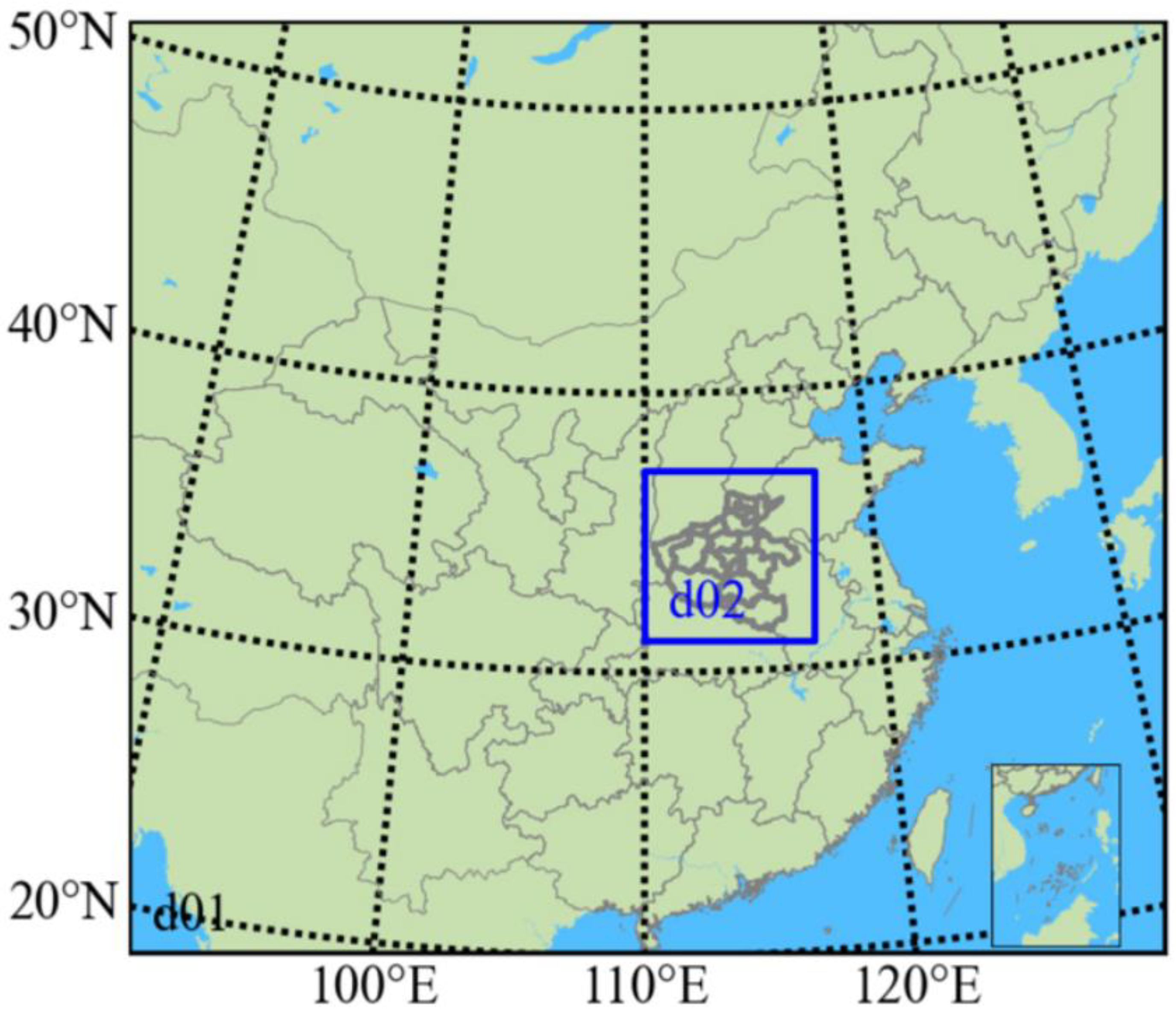
2.1. Study Area

Henan is in the middle eastern part of China, near the middle and lower reaches of the Yellow River, between 31°23′–36°22′ north latitude and 110°21′–116°39′ east longitude. It has a warm temperate–subtropical, humid–semi-humid monsoon climate, with an average annual precipitation of about 500~900 mm. Henan Province is hot in summer with abundant rainfall. The annual average air temperature in the province is typically 12–16 °C, with a large annual air temperature and daily range. The altitude of Henan Province is generally high in the east and south and low in the west and north. The difference between the mountains and plains is obvious, and the elevation of the province is 23.2–2413.8 m. The primary industry of Henan Province takes up a large proportion, and changes in the natural environment such as climate will have a great impact on agricultural production.

2.2. Dataset

2.2.1. Meteorological Data

The basic meteorological data from 1978 to 2017 come from the China Meteorological Forcing Data Sharing Service System (http://data.cma.cn accessed on 10 November 2022). There are 124 weather stations in Henan Province. The data in this paper include daily minimum (T_min), maximum (T_max), and mean (T) air temperature (°C); average pressure (P, kPa); relative humidity (RH, %); sunshine hours (n, h); and average wind speed (u, m s⁻¹).

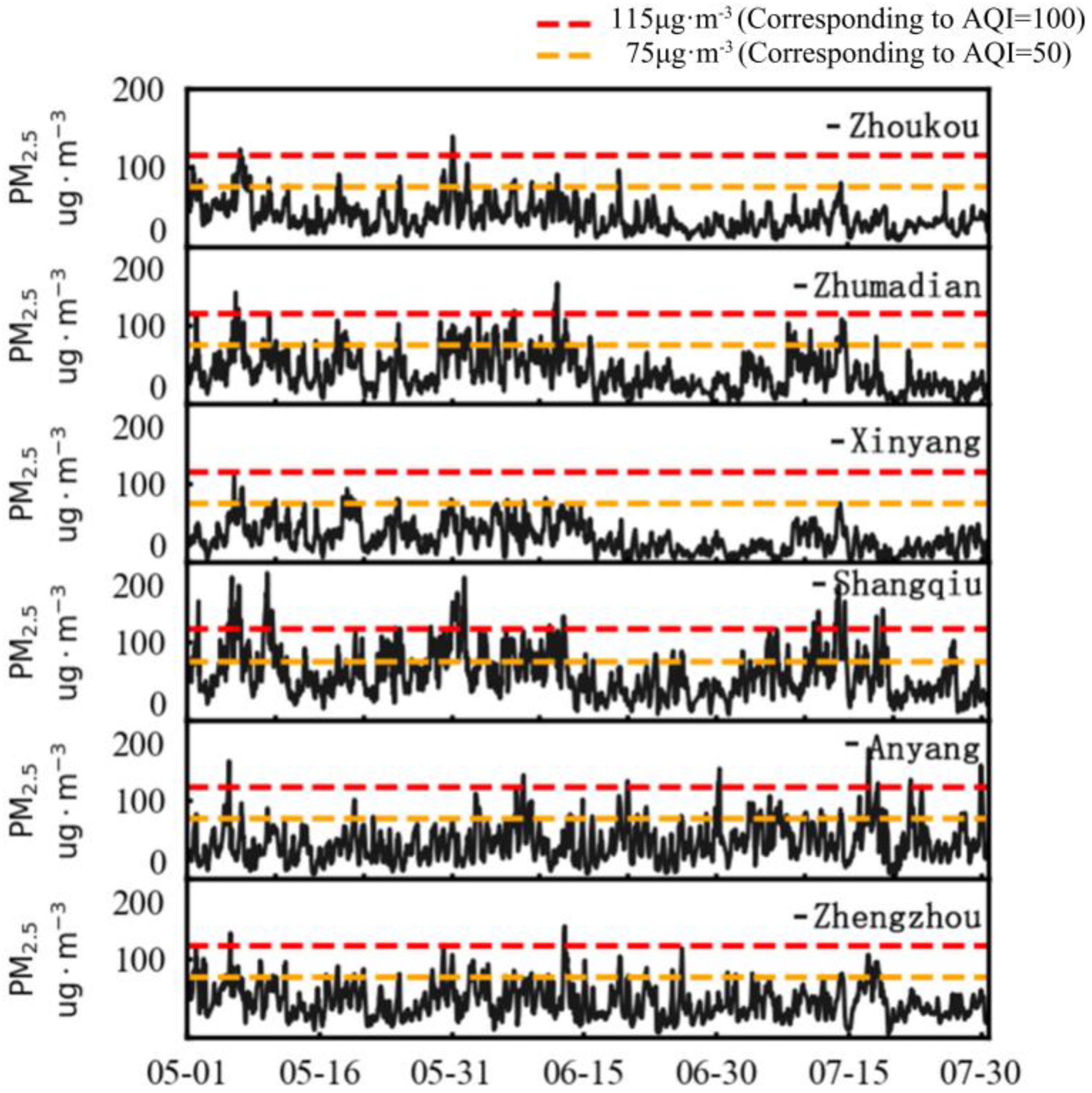
2.2.2. Air Quality Data

Hourly concentration data of six conventional pollutants (e.g., PM2.5, PM10, O₃, NO₂, SO₂, and CO) during 20 May 2016–20 June 2016 were extracted from the China National Environmental Monitoring Center and the national urban air quality real-time release platform. Seventeen (except for Jiyuan) national air quality automatic monitoring stations have been established in Henan Province. In this study, the observational data from Jiaozuo are used to replace the Jiyuan air quality data.

2.2.3. Final (FNL) Reanalysis Data

FNL reanalysis data [32] are used to drive the operation of the Weather Research and Forecasting (WRF) model. This product comes from the GDAS (Global Data Assimilation System) of the NCEP (National Center for Environmental Prediction). The GDAS system covers all regions of the world, with a spatial resolution of 1° × 1° and a time resolution of 6 h. It assimilates ground observations, satellite observation data, sounding ball data, and aircraft observation data.

2.2.4. Emissions Listing

To describe the pollutant-concentration-change trend in China and Henan Province more reasonably and accurately, the emission inventory used in this study is derived from the Multi-resolution Emission Inventory for China (MEIC, http://meicmodel.org/ accessed on 10 November 2022) [33,34,35,36]. The total emissions of PM_2.5, PM₁₀, CO, SO₂, NO_x, BC, OC, NH₃, and VOCs in Henan Province in 2016 were 49.2, 66.8, 815.1, 53.0, 130.6, 8.2, 11.8, 97.3, and 1.462 million tons, respectively. The chemical mechanism is selected as CB05.

3. Methods

3.1. Calculation of Reference Evapotranspiration

The Penman–Monteith (PM) model is the reference crop evapotranspiration (ET₀) calculation method recommended by FAO-56 in 1998. Based on the principles of energy balance and aerodynamics, this model has a relatively complete theoretical basis and high calculation accuracy and has been widely used in the world. In this study, the PM model is used to calculate ET₀ of the daily timescale and day–night timescale, respectively.

ET₀ of the daily timescale can be calculated by Equation (1) [37]:

$$E{T}_0=\frac{0.408\mathrm{\Delta }\left(R_n-G\right)+\gamma \frac{900}{T + 273}{u}_2\left(e_s-e_a\right)}{\mathrm{\Delta }+\gamma \left(1+0.34u_2\right)}$$

(1)

where $E{T}_0$ is the daily reference crop evapotranspiration, mm d⁻¹; $G$ is the soil heat flux density, MJ m⁻² d⁻¹; $R_n$ is the crop surface net radiation, MJ m⁻² d⁻¹; $T$ is the air temperature at 2 m above the ground, °C; $e_s$ is the saturated vapor pressure, kPa; $e_a$ is the actual vapor pressure, kPa; $\mathrm{\Delta }$ is the vapor pressure curve slope, kPa °C⁻¹; $\gamma$ is the humidity constant, kPa °C⁻¹; and $u_2$ is the wind speed at 2 m above the ground, m s⁻¹.

According to the research period, the calculation formula of ET₀ on the day–night timescale is slightly different:

$$E{T}_{0-\mathrm{d}}=\frac{0.408\mathrm{\Delta }\left(R_n-G\right)+\gamma \frac{520}{T + 273}{u}_2\left(e_s-e_a\right)}{\mathrm{\Delta }+\gamma \left(1+0.34u_2\right)}$$

(2)

$$E{T}_{0-\mathrm{n}}=\frac{0.408\mathrm{\Delta }\left(R_n-G\right)+\gamma \frac{370}{T + 273}{u}_2\left(e_s-e_a\right)}{\mathrm{\Delta }+\gamma \left(1+0.34u_2\right)}$$

(3)

where $E{T}_{0-\mathrm{d}}$ is the reference crop evapotranspiration in day time, and $E{T}_{0-\mathrm{n}}$ is the reference crop evapotranspiration during night. The meaning of other parameters is the same as Equation (1).

3.2. Online Two-Way Coupling of WRF–Chem

3.2.1. Model Setting

The simulation time of this study is May and June 2016, and the study area is set at 36.5° N, 110° E as the center, and the first and second standard latitudes are 20° N and 30° N, respectively. Two layers are nested in the simulated region (Figure 1). The first layer covers all regions of China with a resolution of 27 × 27 km² and a grid number of 148 × 133 from east to west. The second layer covers all cities in Henan Province with a resolution of 9 × 9 km² and a grid number of 72 × 72 from east to west. The model adopts a terrain-following coordinate system with 35 vertical layers. To more reasonably describe the vertical change characteristics of meteorological elements and pollutant concentration in the boundary layer, the number of vertical layers in the boundary layer is encrypted, and the boundary layer includes 9 to 13 layers below.

The hourly meteorological elements of WRF–Chem, such as air temperature, air pressure, humidity, wind direction, and wind speed, are provided by the mesoscale meteorological model WRFv4.1.3. The simulation period is from 10 May 2016 to 20 June 2016, the first 10 days are the initialization time of the mode, and the simulation results after 20 May 2016 are used for analysis. The integral time step is 5 min, and the output frequency is 1 h. Simulation results of the global model MOZARTv2.4 are adopted for the initial boundary conditions. Since PM2.5 is the main pollutant in summer air in Henan Province, this experiment mainly simulates PM2.5 to represent the influence of aerosol changes during this period. The simulated PM2.5 included sulfates, ammonium salts, nitrates, organic matter, black carbon, primary PM2.5, sand, and sea salt.

3.2.2. Experimental Design

Based on the variation trend of PM2.5 concentration in Zhoukou, Zhumadian, Xinyang, Shangqiu, Anyang, and Zhengzhou from May to July 2016 (Figure 2), it can be seen that light pollution is the main focus from May to July, and some cities such as Shangqiu, Zhumadian, and Zhoukou can reach medium pollution in certain periods. When the pollution is heavy, the particulate concentration in the atmosphere can change the solar radiation reaching the ground and change the meteorological elements (e.g., temperature, humidity, and wind speed) in the atmosphere. This study selected 20 May 2016–20 June 2016 as the study period to quantitatively evaluate the effects of particulate concentration in the atmosphere on meteorological elements and ET₀ by comprehensively considering the pollution level and the growth process of crops.

The online two-way coupling experiment design is shown in

Table 1. Experimental design.

	Date	Group	Simulation of Meteorological Elements
Initialization	10 May 2016–19 May 2016	fb: contains all meteorological and chemical processes as well as aerosol radiation and feedback fdda: assimilates meteorological observations nofb: shuts down the emission source for simulation	air temperature at 2 m (T), relative humidity (RH), air pressure (P), and wind speed at 10 m(u), short-wave radiation (SW), and long-wave radiation (LW)
Analysis	20 May 2016–20 June 2016

. The simulation experiment includes an aerosol feedback group (fb), a control group with observations assimilation (fdda), and a non-aerosol feedback group (nofb). The fb group and the fdda group are compared to test the simulation accuracy, and fb minus nofb can produce the effects of aerosol on different meteorological elements. The meteorological data of fb group and the nofb group are used to calculate ET_0-fb and ET_0-nofb, respectively. ET_0-fb minus ET_0-nofb is the effect of aerosol on ET₀ (ΔET₀).

3.3. Simulation Evaluation

The coefficient of determination (R²) is mainly used to measure the linear correlation between two variables. It can be calculated by

$$R^2=\frac{{\left({\displaystyle \sum _{i=1}^n\left(O_i-\overline{O}\right)\left(P_i-\overline{P}\right)}\right)}^2}{{\displaystyle \sum _{i=1}^n{\left(O_i-\overline{O}\right)}^2{\displaystyle \sum _{i=1}^n{\left(P_i-\overline{P}\right)}^2}}}$$

(4)

where O_i and P_i represent the observed value and simulated value corresponding to a given variable, respectively. $\overline{O}$ and $\overline{P}$ represent the corresponding average values, respectively, and n represents the total amount of samples.

Normalized mean bias (NMB) is used to normalize the mean deviation to avoid excessive dispersion of the observed value range. It can be calculated by

$$NMB=\frac{{\displaystyle \sum _{i=1}^n\left(P_{x,t}^i-O_{x,t}^i\right)}}{{\displaystyle \sum _{i=1}^n{O}_{x,t}^i}}\times 100\%$$

(5)

where $O_{x,t}^i$ is the ith observation value at point x and time t, $P_{x,t}^i$ is the ith simulated value at point x and time t, and n is the total number of samples.

4. Results Analysis

4.1. Verification of Simulation Accuracy

The air temperature at 2 m, the wind speed at 10 m, and the time series of the relative humidity and air pressure observed by 124 ground stations were used to evaluate the simulation results of the online two-way coupling of the WRF–Chem experiment. Herein, 2 m air temperature, 10 m wind speed, and relative humidity used hourly data. Due to the lack of hourly observational data on air pressure, daily observational data were used for verification.

Table 2. Simulation accuracy verification.

City	T		u		RH		P
	R2	NMB	R2	NMB	R2	NMB	R2	NMB
Anyang	0.906	12.11%	0.700	−32.61%	0.888	−18.03%	0.998	0.47%
Hebi	0.906	12.14%	0.643	−24.87%	0.825	−22.09%	0.998	−0.78%
Jiaozuo	0.902	15.21%	0.670	−11.63%	0.830	−35.86%	0.997	0.01%
Kaifeng	0.890	13.61%	0.574	−0.04%	0.813	−17.40%	0.997	−0.01%
Luoyang	0.889	13.12%	0.540	−10.04%	0.805	−18.22%	0.996	0.06%
Nanyang	0.911	12.99%	0.662	−15.20%	0.861	−15.14%	0.998	−0.15%
Pingdingshan	0.884	14.35%	0.580	−8.87%	0.794	−16.53%	0.997	−0.22%
Puyang	0.908	11.63%	0.640	−5.54%	0.831	−28.75%	0.998	−0.01%
Sanmenxia	0.907	15.16%	0.512	−27.07%	0.797	−13.03%	0.995	−0.40%
Shangqiu	0.904	11.07%	0.590	13.82%	0.823	−21.28%	0.998	−0.02%
Luohe	0.896	15.33%	0.654	17.15%	0.755	−18.37%	0.997	0.01%
Xinxiang	0.903	13.66%	0.672	−8.18%	0.862	−20.40%	0.997	−0.01%
Xinyang	0.889	12.36%	0.705	6.21%	0.845	−18.07%	0.997	0.53%
Xuchang	0.893	16.12%	0.572	−5.87%	0.780	−19.23%	0.997	0.04%
Zhengzhou	0.887	13.69%	0.591	−2.83%	0.829	−18.23%	0.997	1.44%
Zhoukou	0.890	11.89%	0.572	24.13%	0.819	−11.87%	0.998	−0.02%
Jiyuan	0.905	10.12%	0.541	17.69%	0.815	16.28%	0.997	−0.18%
Zhumadian	0.916	13.96%	0.619	8.84%	0.831	−13.26%	0.998	−0.06%

shows the accuracy verification of the simulation test. Compared with the observed values of air temperature and air pressure, R² was above 0.88, and NMB was within 16.5% and 1.5%, respectively. The simulation accuracy of wind speed and relative humidity was slightly lower: R² was above 0.5 and 0.75, and NMB was within −36%, respectively. As can be seen from the online two-way coupling simulation experiment, the simulation results of the air temperature of each city were overestimated, the simulation accuracy of air pressure was significantly higher than other meteorological elements, and the simulation results of wind speed and relative humidity in most cities were underestimated. The wind speed simulation results of Anyang, Hebi, Zhoukou, and Sanmenxia had a large deviation; among them, the wind speed simulation results of Anyang, Hebi, and Sanmenxia were underestimated (NMB < −20%), while the wind speed simulation results of Zhoukou were overestimated (NMB > 20%). The relative humidity of the Hebi, Jiaozuo, Puyang, and Xinxiang simulation results was underestimated (NMB < −20%). Figure 3 shows the comparison between the observed values of different meteorological elements in some cities (Puyang, Kaifeng, Xuchang, Luohe, Zhoukou, and Xinxiang) and the simulated values without aerosol feedback and with aerosol feedback. The results show that online two-way coupling of the WRF–Chem simulation can better represent the fluctuation characteristics and time variation trend of different meteorological elements. Although the simulation results of some stations vary, the overall simulation accuracy is relatively high, and the results are reliable. In summary, WRF–Chem can better simulate the atmospheric conditions from 20 May 2016 to 20 June 2016. In the simulation test, aerosol reduced air temperature in Henan Province by 0.036 °C, and wind speed by 0.176 m/s, air pressure by 20 Pa and increased relative humidity by 1.39%.

4.2. Effects of Aerosol on ET₀

4.2.1. Time Scale

Previous studies of the effects of aerosol ET₀ at time scale are mainly based on the day scale (24 h) and day–night scale comparison. According to the air quality index (AQI), the observed values of cities are classified as excellent (0~50), good (51~100), light pollution (101~150), and medium pollution (151~200) (based on the meteorological observations provided by the National Air Quality Observatory, there was no heavy pollution in Henan Province during this period). In this study, an AQI of 0~100 is classified as an excellent condition, and an AQI of 101~200 is classified as a polluted condition. To better understand the effects of aerosol on ET₀ under different levels of pollution, the daily ΔET₀ of different stations are classified according to the corresponding AQI of their cities and analyzed spatially. As shown in Figure 4, ΔET₀ showed significant spatial differences under two different conditions. In the polluted condition, the ΔET₀ of different stations is −0.545~0.676 mm d⁻¹, and extreme values appear at the Nanle Station (−0.545 mm d⁻¹) and the Gushi Station (0.676 mm d⁻¹). Aerosol shows positive regulation of ET₀ at 75 stations and shows negative regulation at the remaining 49 stations. Figure 4a shows that positive regulation mainly occurs in the eastern, southeastern, and northwestern parts of Henan Province, while negative regulation mainly occurs in the northeastern, central, and western parts of Henan Province. For an excellent condition, the ΔET₀ of different stations is −0.309~0.380 mm d⁻¹, and extreme values appeared at the Weihui Station (−0.309 mm d⁻¹) and the Jili Station (0.380 mm d⁻¹), indicating that the influence of aerosol is lower than that of a polluted condition. Aerosol shows positive regulation of ET₀ at 74 stations and shows negative regulation at the remaining 50 stations. Figure 4b shows that positive regulation mainly occurs in western, southern, and a part of eastern Henan Province, while negative regulation mainly occurs in northern and central Henan Province.

Taking into account the short days and long nights in the Northern Hemisphere from May to June, the period of short-wave radiation (SW) > 0 in the WRF–Chem calculation results is regarded as the day, and the period of SW < 0 is regarded as the night. In this way, the daytime mentioned in this paper is 14 h, from 6:00 to 20:00 Beijing time, and the nighttime is 10 h, from 20:00 to 6:00 Beijing time, because the aerosol function is a continuous process. Under the two different conditions, the spatial pattern of daytime ΔET_0-d and all-day ΔET₀ is similar (Figure 5a,b), while the spatial pattern of nighttime ΔET_0-d is different (Figure 5c,d). In terms of the daytime, the extreme values of ΔET_0-d in a polluted condition appear at the Puyang Station (−0.302 mm d⁻¹) and the Huaibin Station (0.559 mm d⁻¹), respectively. Aerosol shows positive regulation of ET₀ at 68 stations and shows negative regulation at the remaining 56 stations. For an excellent condition, the extreme values of ΔET_0-d for different stations appear at the Zhongmu Station (−0.325 mm d⁻¹) and the Shangcai Station (0.306 mm d⁻¹). Aerosol shows positive regulation of ET₀ at 78 stations and shows negative regulation at the remaining 46 stations. Compared with an excellent condition, the influence of aerosol on ΔET_0-d in a contaminated condition shows a stronger positive regulation, while the negative regulation is closer.

At night, due to the disappearance of solar short-wave radiation, surface energy continues to escape to the outside world in the form of long-wave radiation, and the net surface radiation at night becomes negative. However, due to the existence of the atmosphere and aerosol, long-wave radiation cannot completely escape to outer space, and part of long-wave radiation still returns to the ground in the form of atmospheric inverse radiation, thereby reducing the loss of ground energy at night. This process is influenced by the microclimate and topography, which also explains the spatial difference between nighttime ΔET_0-n and daytime ΔET_0-d under a polluted condition. As shown in Figure 5c, the extreme values of ΔET_0-n appeared at the Mianchi Station (−0.342 mm d⁻¹) and the Fanxian Station (0.140 mm d⁻¹) under a polluted condition. As shown in Figure 5d, the extreme values of ΔET_0-n appeared at the Shangjie Station (−0.325 mm d⁻¹) and the Gushi Station (0.306 mm d⁻¹) under an excellent condition. Overall, for polluted conditions, positive regulation mainly occurred in the eastern, central, and a few areas in northern and southeastern Henan Province, while negative regulation mainly occurred in the northern, western, and a few areas in eastern Henan Province. For an excellent condition, the central region still mainly showed positive regulation, and only a few areas showed negative regulation. As observed, aerosol shows positive regulation of ET₀ at 109 stations for an excellent condition and shows negative regulation at 81 stations in a polluted condition, which means that the positive regulation of aerosol on ET_0-n is stronger in more areas than in a polluted condition.

Due to the influence of natural factors such as topography and human factors such as economic development, air pollution has regional characteristics. As shown in Figure 6, the effects of aerosol on ET₀ are different in different cities. The clustering analysis of cities is consistent with the spatial analysis results in Figure 4 and Figure 5. For polluted conditions, the diurnal influence of aerosol varies the most between cities, and Puyang has the highest value of negative regulation, indicating that the impact of aerosol in this area has reduced ET₀ to the greatest extent. Zhoukou has the highest value of positive regulation, that is, the impact of aerosol in this area has increased ET₀ to the greatest extent. Notably, in this study period, Xinyang showed light pollution only for one day (June 12), and the AQI was less than 100 for the rest of the period. Due to the small sample size, Xinyang’s analysis results may be underestimated or overestimated in a polluted condition, but the analysis results under an excellent condition are still reliable. The results of cluster analysis show that the effects of aerosol show little difference between the whole day and the daytime under an excellent condition, which also conforms to the spatial pattern with highly similar time scales in Figure 4 and Figure 5. Meanwhile, although the daily and day-time aerosol effects in a polluted condition are divided into one category, and spatial analysis also shows that the two groups have similar spatial distribution characteristics, as the specific differences in the two timescales between cities are still obvious. At night, ET_0-n is affected by radiation and decreases, as the effects of aerosol on ET_0-n are weaker than those in the daytime, and the difference in the effects of aerosol at night is not obvious under the two conditions.

4.2.2. Radiation and Aerodynamic Terms

The P-M formula for ET₀ is a synthesis of radiation and aerodynamic factors, and aerosol affects both. As for radiation, the forcing of aerosol radiation affects the surface energy budget to a great extent. In terms of airflow, the existence of aerosol affects the boundary layer height and horizontal airflow. The mechanism of aerosol affecting ET₀ is easy to understand by analyzing the effects of aerosol on radiation (ET_0-R) and aerodynamic terms (ET_0-A) of ET₀ in Henan Province.

Figure 7 shows the spatial analysis of the numerical variation of the radiation (Figure 7a) and aerodynamic (Figure 7b) terms of ET₀ of different stations in Henan Province under the influence of aerosol. The ΔET_0-R of different stations is −0.180–0.200 mm d⁻¹, the ΔET_0-R of 38 different stations is negative, and the ET_0-R of the remaining 86 stations is increased. As observed, significant changes have taken place in ET_0-R in some areas in the eastern and southern Henan Province. Aerosol shows negative regulation of ET_0-R mainly appearing in the eastern region and shows positive regulation mainly appearing in the southern region. The ΔET_0-A of different stations is −0.260~0.598 mm d⁻¹, which is more variable than ΔET_0-R; the ΔET_0-A of 32 stations is negative, and aerosol has a positive regulation on the ΔET_0-A of the remaining 92 stations. Meanwhile, aerosol shows positive regulation of ET_0-A high-value regions mainly appearing in the eastern region, which is highly overlapped with the negative regulation regions of ET_0-R, while aerosol shows negative regulation of ET_0-A high-value regions mainly appear in the parts of northern, central, southern, and western parts of Henan Province, and there is no obvious distribution pattern.

Figure 8 shows the numerical changes of ET_0-R and ET_0-A in Henan Province’s cities with and without aerosol feedback. Figure 8a shows the overall change in ET_0-R and ET_0-A in the whole period of 20 May 2016 to 20 June 2016. Under the influence of aerosol, the cities in Henan Province have obvious differences in ET_0-R and ET_0-A. The average ΔET_0-R of each city is −0.159~0.169 mm d⁻¹, and the average ΔET_0-A is −0.118–0.449 mm d⁻¹. The values of ΔET_0-R in 16 cities are positive, indicating that the influence of aerosol increases the values of ET_0-R in these areas. The values of ΔET_0-A in 10 cities are negative, indicating that the influence of aerosol decreases the value of ET_0-A in these areas. According to ΔET_0-R and ΔET_0-A of different cities, Zhoukou, Zhengzhou, Shangqiu, and Pingdingshan, the increase in ΔET_0-A in Nanyang and Luoyang is the main reason for the increase in ET₀ in these cities. The decrease in ΔET_0-A in Xuchang, Xinxiang, Sanmenxia, Puyang, Luohe, Kaifeng, Hebi, and Anyang is the main reason for the decrease in ET₀ in these cities, while the increase in ΔET_0-R of Zhumadian and Jiaozuo leads to the increase in ET₀. Overall, during the period from May 20th to June 20th, ΔET_0-A in most areas under the influence of aerosol will have greater changes, which will dominate the change in ET₀. Figure 8b,c compare ΔET_0-R and ΔET_0-A in a polluted condition and an excellent condition, respectively. As observed, significant changes have taken place in ΔET_0-R and ΔET_0-A in a polluted condition and an excellent condition. In a polluted condition, for a total of eight cities in the province, ΔET_0-A dominated the increase in ΔET₀, while the decrease in ΔET_0-A in Sanmenxia, Puyang, and Nanyang led to the corresponding decrease in ΔET₀. In an excellent condition, for a total of eight cities in the province, ΔET_0-A dominated the increase in ΔET₀, and, for seven cities, ΔET_0-A dominated the decrease in ΔET₀. In contrast, the leading role of ΔET_0-R was not obvious. Comparing the analysis results on a daily scale from Figure 6, Figure 8 explains the causes of the daily scale of ΔET₀ of each city in the two scenarios. In this regard, a preliminary summary of the above phenomenon can be made: during May and June 2016, the change in ΔET_0-A under the influence of aerosol is the main reason for the change in ET₀ in Henan Province. Compared with the full-time and excellent conditions, the ET₀ in more cities (5) under a polluted condition is mainly affected by ΔET_0-R; compared with a polluted condition, ΔET_0-A dominates the ET₀ changes in more cities (15) under an excellent condition.

5. Discussion

In 2002, Rodrick et al. pointed out that ET₀ changes in Australia and New Zealand were largely affected by increased cloud cover and aerosol concentrations in the Southern Hemisphere [38]. However, they did not calculate the impact. In this study, online two-way coupling of a WRF–Chem experiment was used to simulate variations of different meteorological elements in Henan Province during May and June under the influence of aerosol in 2016; the accuracy of the simulation results is verified by meteorological observation data, and the variation of ET₀ in the whole province under the influence of aerosol is analyzed. As observed, aerosol causes obvious changes in ET₀ in Henan Province during May and June 2016. These results can facilitate an understanding of the variation of aerosol ET₀ and its response mechanism and provide a new idea for agricultural meteorology research.

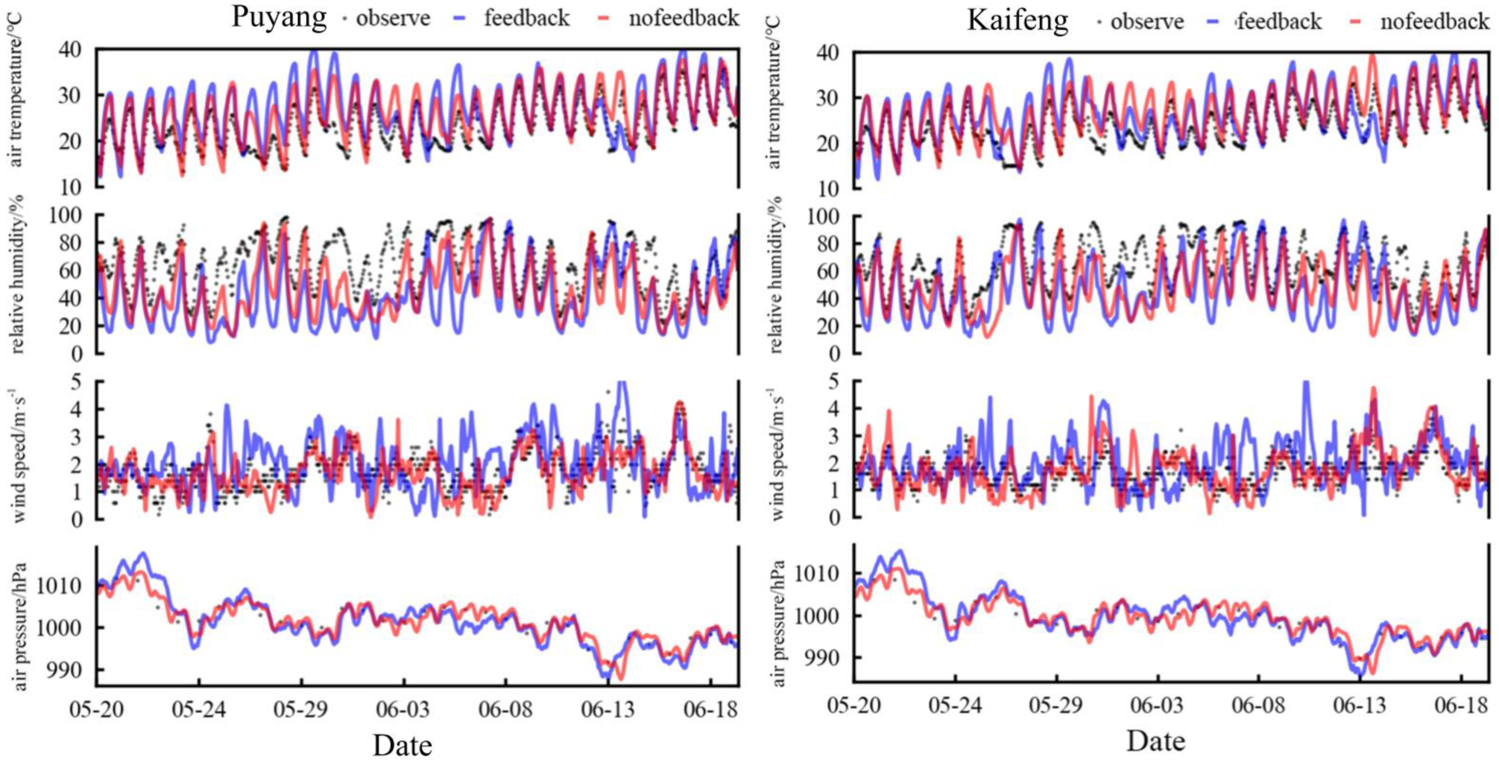
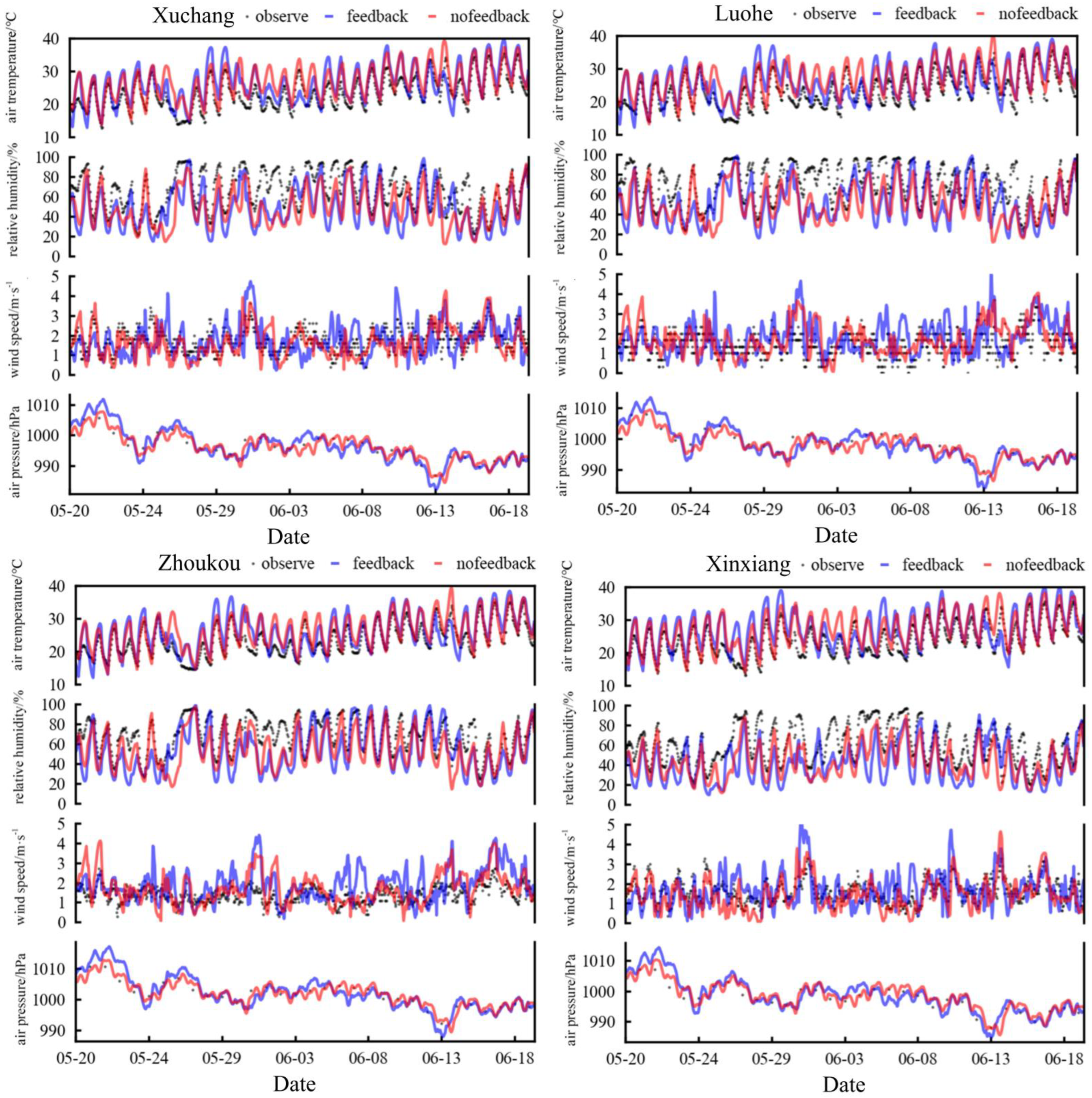
5.1. Meteorological Elements Simulation Accuracy

The longitude, latitude, and elevation of all stations involved in this study were extracted from the Meteorological Information Center of China National Meteorological Administration. During the research, it was found that the simulated data of basic meteorological elements extracted from the online two-way coupling of the WRF–Chem simulation results are quite different from the actual observation data. This can be attributed to the fact that the simulation results of WRF–Chem at each point cannot achieve sufficient accuracy. In this study, the cell grid value of the different stations in the simulation results was used as the simulated value of the meteorological elements of the station, and it was found that the simulation accuracy has been greatly improved (R² increased by 0.5, and NMB decreased by 30%).

5.2. Mechanism of Aerosol Affecting ET₀

During May and June 2016, the change degree of ET₀ in a polluted condition is greater than that in an excellent condition. In the whole province, the extreme value of ΔET₀ becomes higher in a polluted condition. This fully shows that the effects of aerosol on ET₀ are closely related to aerosol concentration, but a simple linear relationship cannot explain the correlation between aerosol concentration and ET₀ changes. With the increase in aerosol concentration, the ET₀ in western Henan Province changes from increasing to decreasing, while the ET₀ in some parts of northwestern Henan Province changes from decreasing to increasing. Increased air pollution will reduce the solar radiation reaching the ground during the day and reduce the loss of long-wave radiation, which is an important reason for the changes in air temperature. Additionally, the direct and indirect effects of different aerosol components are different. When the aerosol components are not uniformly distributed in time and space, the changes in meteorological elements also show differences. These factors work together to make ΔET₀ present a completely different spatial pattern in the two situations.

For an excellent condition, aerosol shows a more general positive regulation of ET_0-d and ET_0-n. The 30-day simulation results show that 55% of stations have ΔET_0-d greater than 0, 65% of stations have ΔET_0-n greater than 0 in polluted conditions, and, for an excellent condition, the proportions of stations with ET_0-d and ET_0-n greater than 0 are 63% and 88%, respectively. ET_0-A plays a leading role in the change in ET₀ in most areas of Henan Province. In the study period, whether positive regulation or negative regulation, ΔET_0-A always determines the positive and negative values of ΔET₀ in most cities, and this phenomenon becomes more significant in an excellent condition. This phenomenon cannot deny the effect of aerosol on the regulation of ET_0-R. During May and June, the sun in the Northern Hemisphere directly points near the Tropic of Cancer, and solar radiation provides enough energy that aerosol still has enough energy to “heat” the ground after cutting through the radiation. Meanwhile, with the aggravation of pollution, ET_0-R began to dominate the change in ET₀ in more cities. This further indicates that when air pollution is heavy enough, the effects of aerosol on ET₀ also tend to regulate radiation terms.

5.3. Uncertainties of the Study

The online two-way coupling experiment takes the presence of aerosol as the only variable (for example, haze is not included in this paper, but haze also has an impact on ET₀), so the change in ET₀ in this test can be completely attributed to the direct and indirect effects of aerosol in the paper. The simulation results of this test are generally reliable, but there are still some uncertainties.

First, the number of stations determines the accuracy of simulation results. The number of available radiation stations in Henan Province is far less than that of ordinary meteorological observation stations, and the simulation accuracy of short-wave and long-wave radiations cannot be fully tested. Additionally, each city has only one available aerosol observation station. On the one hand, when the geographic area of some cities is too large, and the topography is more complex, the reliability of using the aerosol observations of a single radiation as the city average will be reduced. On the other hand, the distribution of aerosol space is uneven. When the variation of urban meteorological elements and ET₀ is investigated, it is reasonable to classify conditions according to urban AQI, while radiation is analyzed, so the rationality of this classification method needs to be verified.

Meanwhile, no heavy pollution occurred in Henan Province’s cities during the study period, so the change in different meteorological elements under heavy pollution situations could not be simulated. However, the effects of aerosol on ET₀ in heavy pollution can only be predicted based on existing results.

Additionally, the WRF–Chem simulation will be restricted by many factors. For instance, WRF–Chem has a poor simulation effect on rainfall, especially meteorological elements during continuous rainfall. When there is obvious rainfall in the weathering process, the analysis results of this period are likely to have a large deviation. Currently, in research using WRF–Chem for simulation, there are almost no continuous simulations for more than one month. In this study, the meteorological conditions of Henan Province in various periods were comprehensively considered, and the longest possible simulation period was selected under the conditions of ensuring the stability of the meteorological environment, to ensure the reliability of the simulation results and the rationality of the analysis results to the greatest extent.

6. Conclusions

This study used the WRF–Chem air quality model to simulate temperature, wind speed, relative humidity, air pressure, short-wave radiation, and long-wave radiation with online two-way coupling feedback, the changes of ET₀ under the influence of aerosol are quantified, and the response mechanism of ET₀ to aerosol is analyzed. The conclusions can be drawn:

(1)

In the online two-way coupling experiment, the simulation results of air temperature and air pressure are better than those of wind speed and relative humidity. WRF–Chem better simulated the fluctuation characteristics and time variation trend of different meteorological elements in Henan Province during May–July 2016, so this method is proven to be reliable for studying the change in ET₀ under the action of aerosol. Aerosol reduces air temperature in Henan Province by 0.036KORENKO, wind speed by 0.176 m/s, and air pressure by 20 Pa and increases relative humidity by 1.39%.

(2)

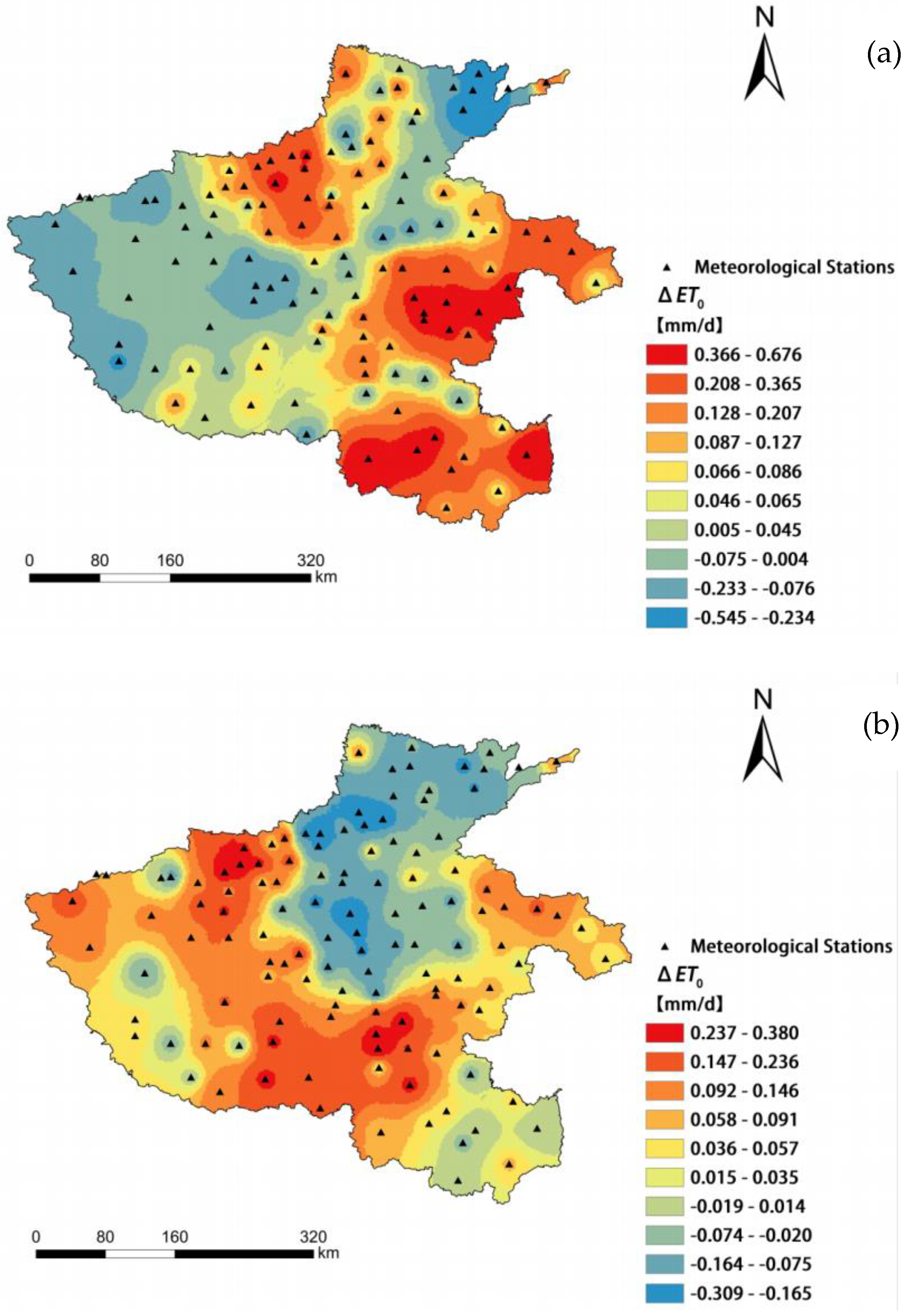
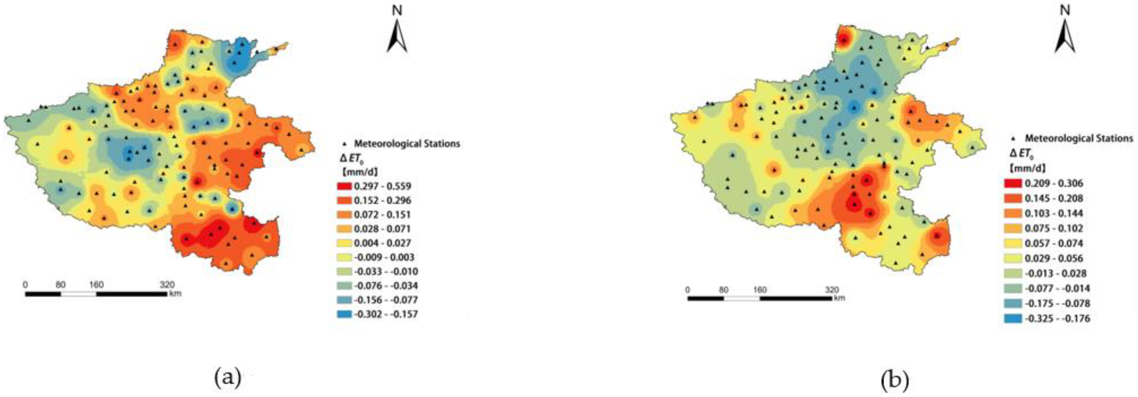
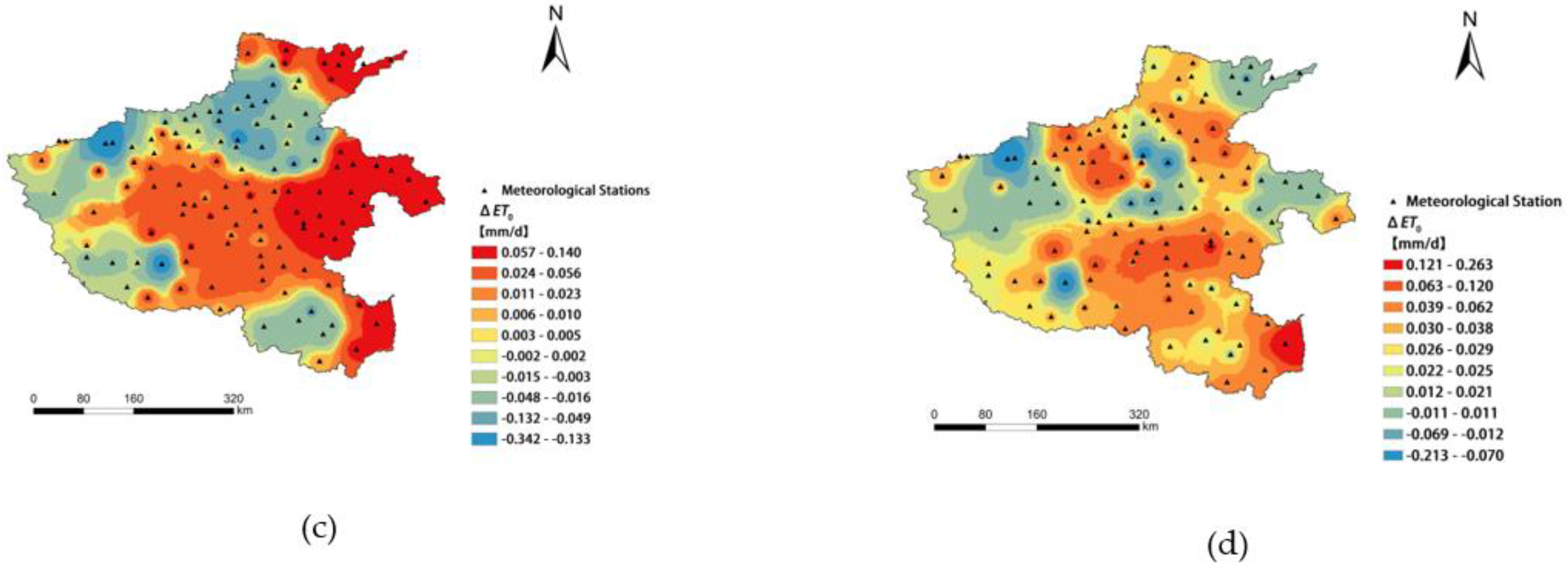
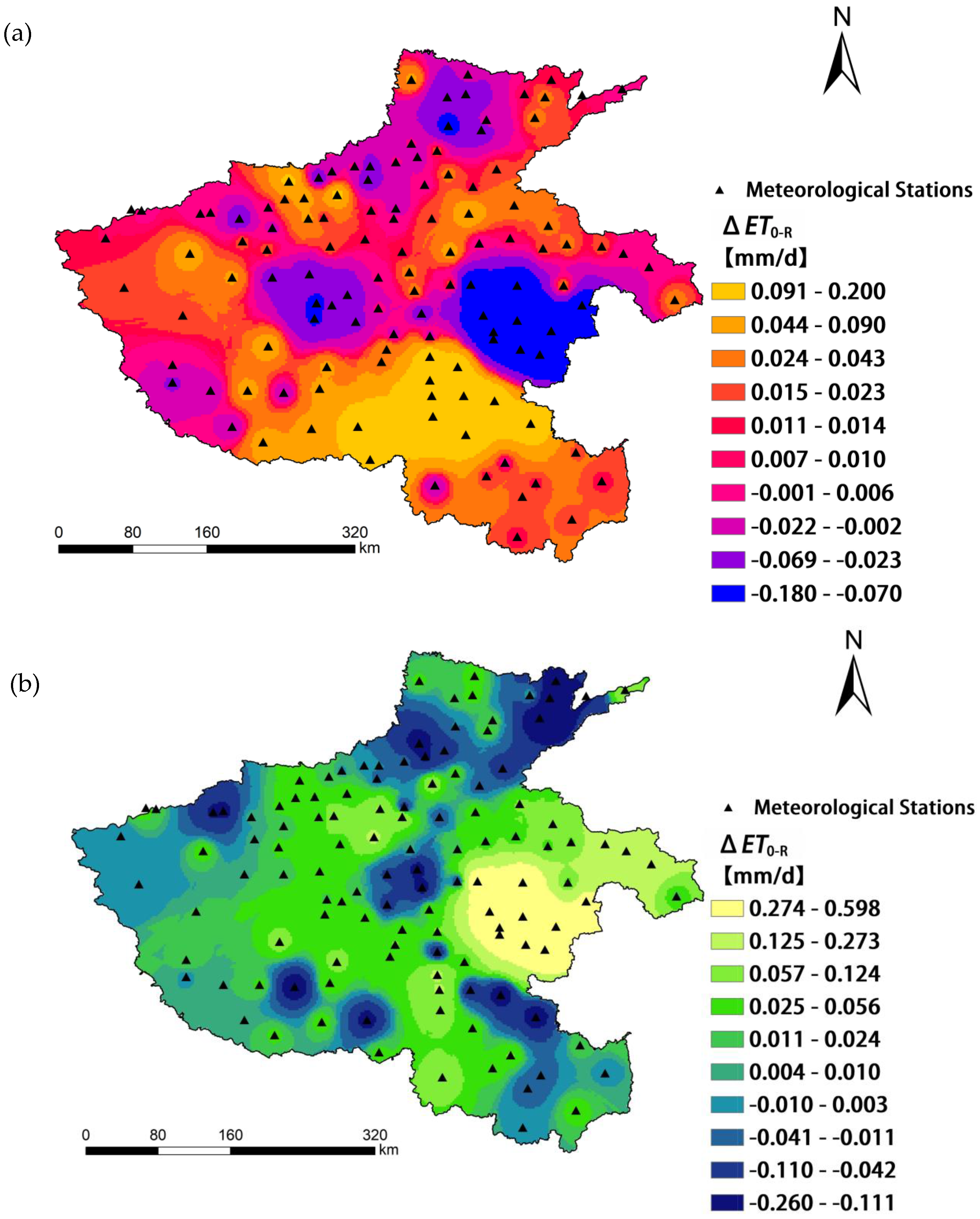
The effects of aerosol on ET₀ are closely related to aerosol concentration. The change degree of ET₀ in a polluted condition is greater than that in an excellent condition. The effects of aerosol on ET₀ vary from region to region, and the spatial pattern of ET₀ changes in contaminative and excellent conditions is quite different. In any condition, the variation of ET_0-d in the whole province is always greater than that of ET_0-n. In an excellent condition, aerosol shows a more general positive regulation of ET_0-d and ET_0-n.

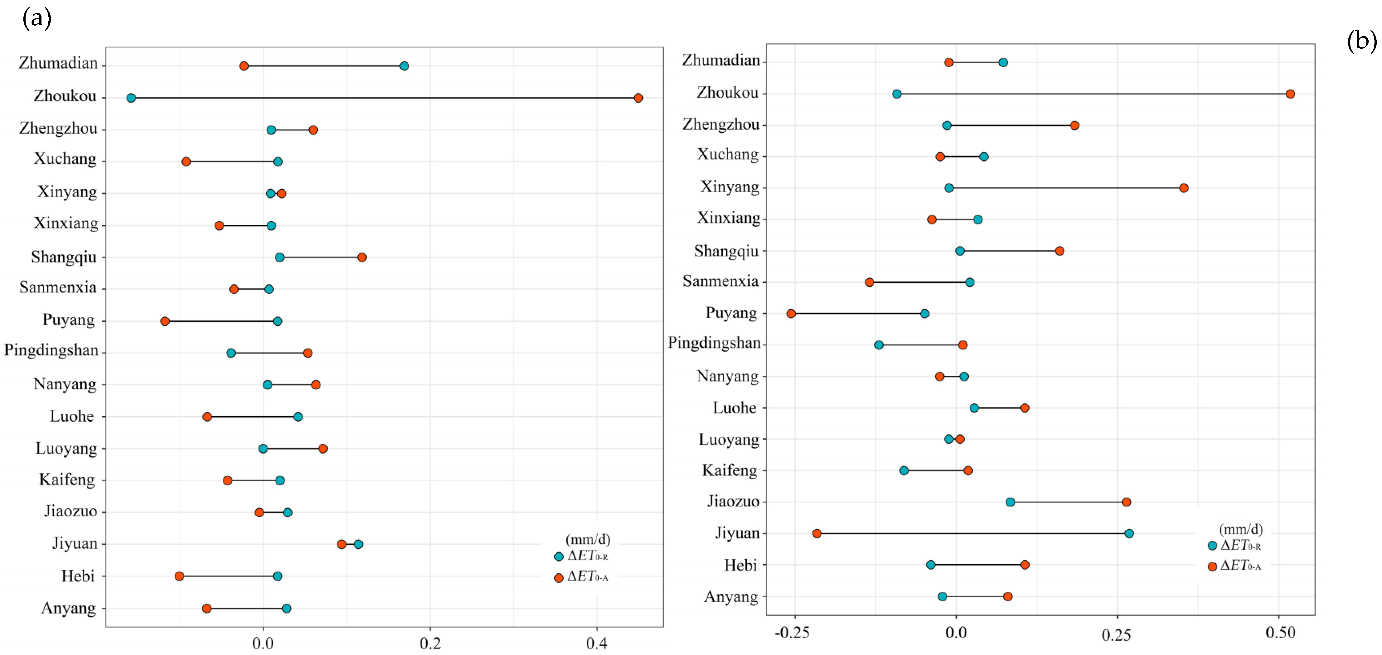
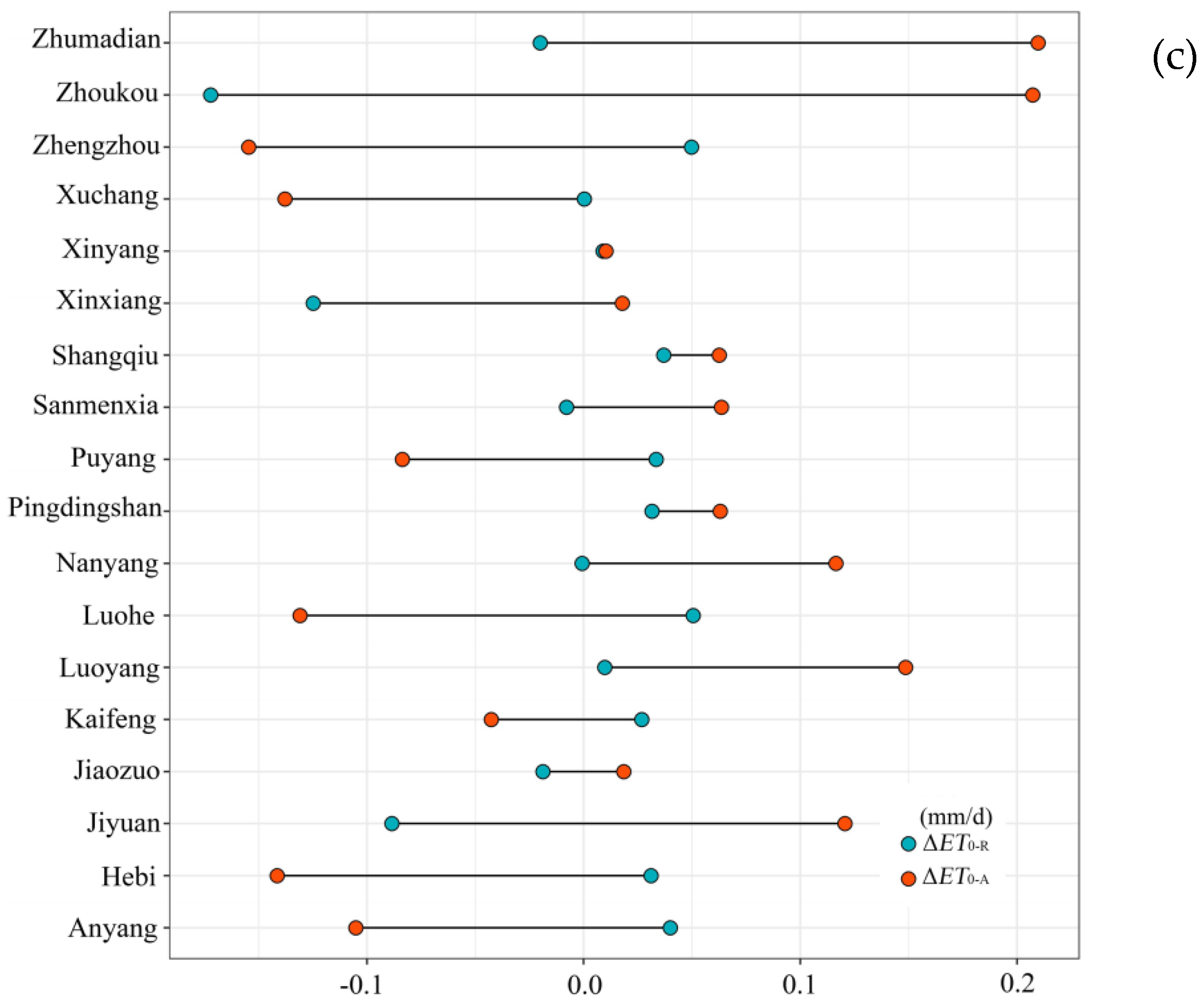
(3)

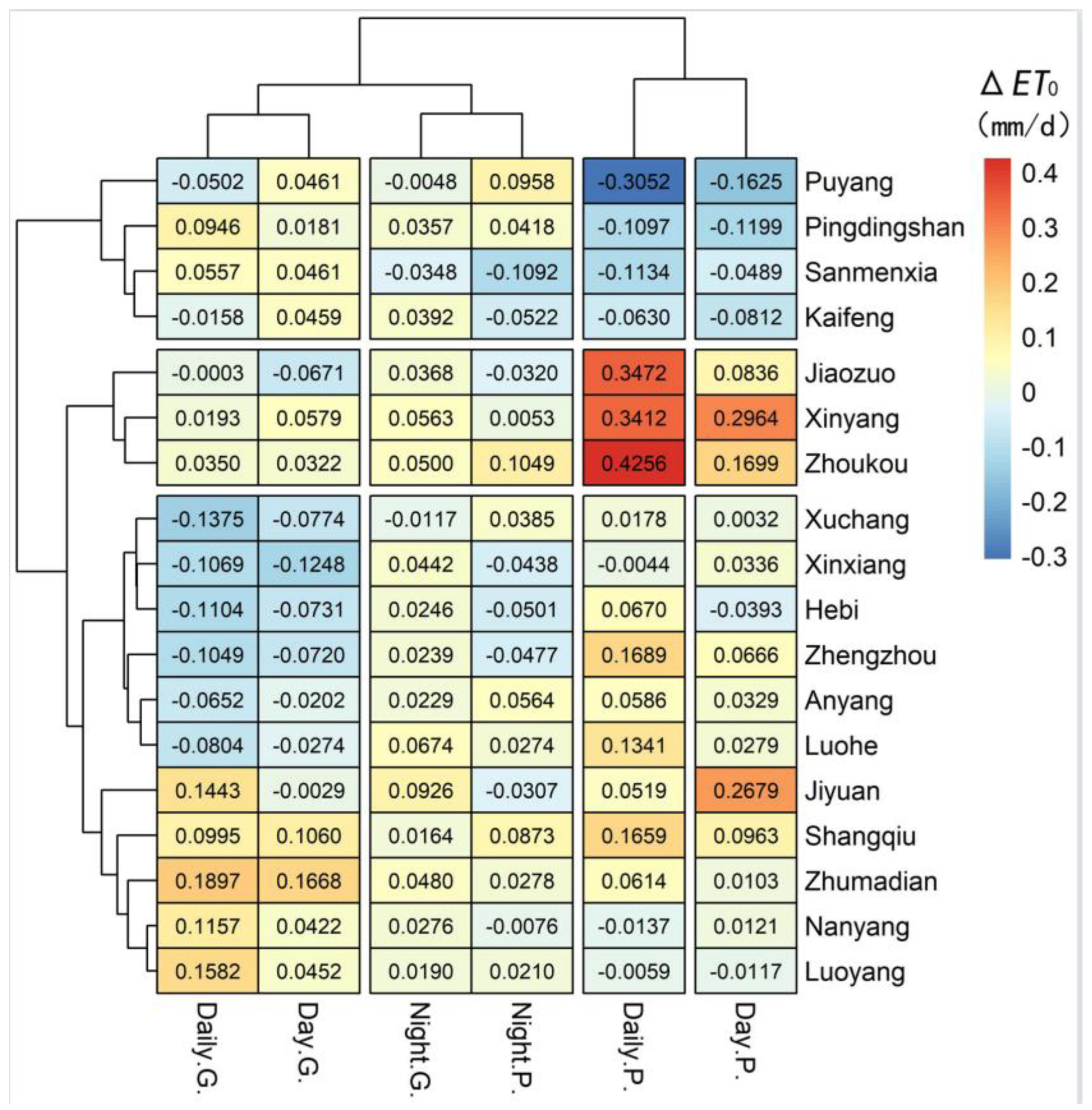
During the study period, ET_0-A played a leading role in the change in ET₀ in most regions of Henan Province. With the increase in pollution, ET_0-R also began to dominate the ET₀ changes in more cities. The cause of this phenomenon is related to the season. In this period, enough surface radiation makes the cooling effect of aerosol not obvious.

The changes and causes of different meteorological elements and ET₀ under the influence of aerosols were investigated to help understand the effects of air pollution on agricultural production and the regional water cycle. In the context of global warming and “darkening”, the effects of aerosol on regional evapotranspiration and agricultural production are more deserving of attention.

References

1. Peng, S.Z.; Xu, J.Z.; Ding, J.L.; Zhang, R.M. Influence of as and bs Values on Determination of Reference Crop Evapotranspiration by Penman-Monteith Formula. J. Irrig. Drain. 2006, 25, 5–8. [Google Scholar]
2. Xu, J.Z.; Peng, S.Z.; Zhang, R.M.; Li, D.X. A neural network model for reference crop evapotranspiration prediction based on weather forecast. J. Hydraul. Eng. 2006, 37, 376–379. [Google Scholar]
3. Wang, S.F.; Wang, S.S.; Duan, A.W.; Liu, Z.D.; Luo, C.Q. Evaluation on Several Methods for Estimating ET0 and Modified Hargeaves Formulas. J. Irrig. Drain. 2010, 29, 29–33. [Google Scholar]
4. Jia, Y.; Cui, N.B.; Wei, X.P.; Gong, D.Z.; Hu, X.T. Modifying Hargreaves model considering radiation to calculate reference crop evapotranspiration in hilly area of central Sichuan Basin. Trans. Chin. Soc. Agric. Eng. 2016, 32, 152–160. [Google Scholar]
5. Xia, X.S.; Zhu, X.F.; Pan, Y.Z.; Zhang, J.S. Influence of Solar Radiation Empirical Values on Reference Crop Evapotranspiration Calculation in Different Regions of China. Trans. Chin. Soc. Agric. Mach. 2020, 51, 254–266. [Google Scholar]
6. Vna, B.; Ge, B.; Ja, B. Multi-step ahead modeling of reference evapotranspiration using a multi-model approach. J. Hydrol. 2019, 3, 581. [Google Scholar]
7. Thomas, A. Spatial and temporal characteristics of potential evapotranspiration trends over China. Int. J. Climatol. 2015, 20, 381–396. [Google Scholar] [CrossRef]
8. Reis, M.M.; Silva, A.J.D.; Junior, J.Z.; Santos, L.D.T.; Lopes, R.M.G. Empirical and learning machine approaches to estimating reference evapotranspiration based on temperature data. Comp. Electr. Agric. 2019, 165, 104937. [Google Scholar] [CrossRef]
9. Villaverde, A.B.A.; Pavón-Domínguez, P.; Carmona-Cabezas, R.; Ravé, E.G.D.; Jiménez-Hornero, F.J. Joint multifractal analysis of air temperature, relative humidity and reference evapotranspiration in the middle zone of the Guadalquivir river valley. Agric. For. Meteorol. 2019, 278, 107657. [Google Scholar] [CrossRef]
10. Zhang, L.; Traore, S.; Cui, Y.; Luo, Y.; Zhu, G.; Liu, B.; Fipps, G.; Karthikeyan, R.; Singh, V. Assessment of spatiotemporal variability of reference evapotranspiration and controlling climate factors over decades in China using geospatial techniques. Agric. Water Manag. 2019, 213, 499–511. [Google Scholar] [CrossRef]
11. IPCC Climate Change 2013—The Physical Science Basis; Cambridge University Press: Cambridge, UK, 2013.
12. Wang, Z.; Yang, L. Delinking indicators on regional industry development and carbon emissions: Beijing-Tianjin-Hebei economic band case. Ecol. Ind. 2015, 48, 41–48. [Google Scholar] [CrossRef]
13. Takemura, T. Simulation of climate response to aerosol direct and indirect effects with aerosol transport-radiation model. J. Geophys. Res. Atmos. 2005, 110, 3–16. [Google Scholar] [CrossRef]
14. Wu, L.; Kaneko, S.; Matsuoka, S. Driving forces behind the stagnancy of China’s energy-related CO2 emissions from 1996 to 1999: The relative importance of structural change, intensity change and scale change. Energy Policy 2005, 33, 319–335. [Google Scholar] [CrossRef]
15. Wang, Y.; Che, H.; Ma, J.; Wang, Q.; Shi, G.; Chen, H.; Goloub, P.; Hao, X. Aerosol radiative forcing under clear, hazy, foggy, and dusty weather conditions over Beijing, China. Geophys. Res. Lett. 2009, 36, L06804. [Google Scholar] [CrossRef]
16. Qin, S.; Liu, F.; Wang, J.; Sun, B. Analysis and forecasting of the particulate matter (PM) concentration levels over four major cities of China using hybrid models. Atmos. Environ. 2014, 98, 665–675. [Google Scholar] [CrossRef]
17. Li, X.; Liu, W.; Chen, Z.; Zeng, G.; Hu, C.; Leon, T.; Liang, J.; Huang, G.; Gao, Z.; Li, Z.; et al. The application of semicircular-buffer-based land use regression models incorporating wind direction in predicting quarterly NO2 and PM10 concentrations. Atmos. Environ. 2015, 103, 18–24. [Google Scholar] [CrossRef]
18. Zhang, Y.; Wen, X.Y.; Jang, C.J. Simulating chemistry–aerosol–cloud–radiation–climate feedbacks over the continental U.S. using the online-coupled Weather Research Forecasting Model with chemistry (WRF/Chem). Atmos. Environ. 2010, 44, 3568–3582. [Google Scholar] [CrossRef]
19. Zhang, Y. Online-coupled meteorology and chemistry models: History, current status, and outlook. Atmos. Chem. Phys. 2008, 8, 2895–2932. [Google Scholar] [CrossRef] [Green Version]
20. Kedia, S.; Cherian, R.; Islam, S.; Das, S.K.; Kaginalkar, A. Regional simulation of aerosol radiative effects and their influence on rainfall over India using WRFChem model. Atmos. Res. 2016, 182, 232–242. [Google Scholar] [CrossRef]
21. Vinoj, V.; Rasch, P.J.; Wang, H.; Yoon, J.H.; Ma, P.L.; Landu, K.; Singh, B. Short-term modulation of Indian summer monsoon rainfall by West Asian dust. Nat. Geosci. 2014, 7, 308–313. [Google Scholar] [CrossRef]
22. Mao, J.J. A Study on Characteristics of Aerosol Inversion and Spatial and Temporal Distribution over East China with MODIS Data. Master’s Thesis, Nanjing University of Information Science and Technology, Nanjing, China, 2011. [Google Scholar]
23. Wang, Z.; Wang, Z.F.; Li, J.; Zheng, H.T.; Yan, P.Z.; Li, J.J. Development of a Meteorology−Chemistry Two-Way Coupled Numerical Model (WRF−NAQPMS) and Its Application in a Severe Autumn Haze Simulation over the Beijing−Tianjin−Hebei Area, China. Clim. Environ. Res. 2014, 19, 153–163. [Google Scholar]
24. Yang, D.D.; Wang, T.J.; Li, S.; Ma, C.Q.; Liu, C.; Yang, F. Air pollution characteristics and source tracking in the Yangtze River Delta based on cruise observation. China Environ. Sci. 2019, 39, 3595–3603. [Google Scholar]
25. Yu, Z.Q.; Ma, J.H.; Cao, Y.; Chang, L.Y.; Xu, J.M.; Zhou, G.Q. Numerical simulations of sources and transport pathways of different PM2.5 pollution types in Shanghai. China Environ. Sci. 2019, 39, 21–31. [Google Scholar]
26. Yu, C.X.; Shi, C.E.; Ling, X.F.; Zhu, J.Y.; Fan, Y. Analysis of a severe fog-haze process in central and eastern China based oncomprehensive observations. Acta Sci. Circumst. 2020, 40, 2346–2355. [Google Scholar]
27. Li, Y.F.; Chen, W.Z. Correlation between aerosol optical depth and ocean primary productivity based on MODIS and CALIOP data. China Environ. Sci. 2017, 37, 76–86. [Google Scholar]
28. Yu, Y.; Wang, Z.H.; Cui, X.D.; Chen, F.; Xu, H.H. Effects of Emission Reductions of Key Sources on the PM2.5 Concentrations in the Yangtze River Delta. Environ. Sci. 2019, 40, 11–23. [Google Scholar]
29. Roderick, M.L.; Farquhar, G.D. The Cause of Decreased Pan Evaporation over the Past 50 Years. Science 2002, 298, 1410–1411. [Google Scholar] [CrossRef]
30. Liu, X.W.; Zhang, X.Y.; Zhang, X.Y. A review of the research on crop responses to the increase in aerial aerosol. Acta Ecol. Sin. 2016, 36, 2084–2090. [Google Scholar]
31. Zhang, X.Y.; Wang, S.F.; Sun, H.Y.; Chen, S.Y.; Shao, L.W.; Liu, X.W. Contribution of cultivar, fertilizer and weather to yield variation of winter wheat over three decades: A case study in the North China Plain. Eur. J. Agron. 2013, 50, 52–59. [Google Scholar] [CrossRef]
32. FNL Reanalysis Data. Available online: https://rda.ucar.edu/datasets/ds083.3/ (accessed on 16 June 2021).
33. Zhang, Q.; Streets, D.G.; Carmichael, G.R.; He, K.B.; Huo, H.; Kannari, A.; Klimont, Z.; Park, I.S.; Reddy, S.; Fu, J.S. Asian emissions in 2006 for the NASA INTEX-B mission. Atmos. Chem. Phys. 2009, 9, 5131–5153. [Google Scholar] [CrossRef] [Green Version]
34. Li, M.; Zhang, Q.; Streets, D.G.; He, K.B.; Zhang, Y. Mapping Asian anthropogenic emissions of non-methane volatile organic compounds to multiple chemical mechanisms. Atmos. Chem. Phys. 2013, 13, 32649–32701. [Google Scholar] [CrossRef] [Green Version]
35. Zheng, B.; Huo, H.; Zhang, Q.; Yao, Z.L.; Wang, X.T.; Yang, X.F.; Liu, H.; He, K.B. High-resolution mapping of vehicle emissions in China in 2008. Atmos. Chem. Phys. 2014, 14, 9787–9805. [Google Scholar] [CrossRef] [Green Version]
36. Liu, F.; Zhang, Q.; Tong, D.; Zheng, B.; Li, M.; Huo, H.; He, K.B. High-resolution inventory of technologies, activities, and emissions of coal-fired power plants in China from 1990 to 2010. Atmos. Chem. Phys. 2015, 15, 18787–18837. [Google Scholar] [CrossRef]
37. Allen, R.G.; Pereira, L.S.; Raes, D.; Smith, M.; Allen, R.G.; Pereira, L.S.; Martin, S. Crop Evapotranspiration Guidelines for Computing Crop Water Requirements; Food and Agriculture Organization of United Nation: Rome, Italy, 1998; p. 56. [Google Scholar]
38. Roderick, M.L.; Farquhar, G.D. Geoengineering: Hazy, cool and well fed? Nat. Clim. Chang. 2012, 2, 76–77. [Google Scholar] [CrossRef]
Figure 1. Location of the simulation area.
Agronomy 13 00082 g001
Figure 2. Time variation of pollutant concentration.
Agronomy 13 00082 g002
Figure 3. Comparisons of observations and model simulations without (blue line) and with (red line) aerosol feedback.
Agronomy 13 00082 g003aAgronomy 13 00082 g003b
Figure 4. Effect of aerosols on ET0 at the daily scale for pollution (a) and good (b) air quality conditions.
Agronomy 13 00082 g004
Figure 5. Effect of aerosols on ET0 during daytime (a,b) and nighttime (c,d) for pollution (a,c) and good (b,d) air quality conditions.
Agronomy 13 00082 g005aAgronomy 13 00082 g005b
Figure 6. Effect of aerosols on ET0 at daily and day-night scales under different pollution conditions in various cities.
Agronomy 13 00082 g006
Figure 7. The effect of aerosol on the ET0 radiation term (a) and aerodynamic term (b).
Agronomy 13 00082 g007
Figure 8. The effect of aerosols on the ET0 radiation term and aerodynamic term values in each city under the full-time (a), pollution (b), and good (c) conditions.
Agronomy 13 00082 g008aAgronomy 13 00082 g008b