Development of Deep Learning Methodology for Maize Seed Variety Recognition Based on Improved Swin Transformer

Abstract

In order to solve the problems of high subjectivity, frequent error occurrence and easy damage of traditional corn seed identification methods, this paper combines deep learning with machine vision and the utilization of the basis of the Swin Transformer to improve maize seed recognition. The study was focused on feature attention and multi-scale feature fusion learning. Firstly, input the seed image into the network to obtain shallow features and deep features; secondly, a feature attention layer was introduced to give weights to different stages of features to strengthen and suppress; and finally, the shallow features and deep features were fused to construct multi-scale fusion features of corn seed images, and the seed images are divided into 19 varieties through a classifier. The experimental results showed that the average precision, recall and F1 values of the MFSwin Transformer model on the test set were 96.53%, 96.46%, and 96.47%, respectively, and the parameter memory is 12.83 M. Compared to other models, the MFSwin Transformer model achieved the highest classification accuracy results. Therefore, the neural network proposed in this paper can classify corn seeds accurately and efficiently, could meet the high-precision classification requirements of corn seed images, and provide a reference tool for seed identification.

1. Introduction

In many countries, corn is not only one of the important food crops, but it also plays an important role in feed production, industrial raw materials, and bioenergy [1,2]. Improving maize production technology can effectively promote the high-quality development of agriculture and drive the growth of the national economy. In the process of agricultural production, seeds are the most basic means of production and the “chip” of agriculture [3,4]. At present, in order to meet the needs of grower recognition of varieties and the different regional environment planting needs, breeders have developed a considerable number of maize varieties. Although these varieties meet the market demand, the risk of mixing seeds is raised. For example, in the process of seed production, processing, storage and transportation, the quality of seed has not been completely effective in detection and control; or in the process of selling seeds, some individuals or enterprises use low-quality corn varieties to fake high-quality corn varieties to make huge profits [5]. All these behaviors will eventually lead to the low purity of seeds. However, the poor purity of maize seeds would potentially reduce the germination rate, seedling rate and disease resistance of maize, evenly affecting the yield of crops and the income of farmers [6]. The accurate identification of seed varieties plays an important role in reducing seed mixing, improving seed purity and ensuring market circulation order. Therefore, it is urgent to explore a nondestructive, efficient and environmental friendly identification method to select high-quality maize seed varieties, provide pure maize seeds for the market and consumers, enhance the international competitiveness of one country’s agricultural products and ensure the sustainable development of agricultural production.

The traditional identification methods of seed purity include the morphological inspection method, field planting inspection method, chemical identification method and electrophoresis technology inspection method [7,8,9,10], however, the above methods are time-consuming, cumbersome in their identification processes and need professional personnel, so they are not suitable for mass analysis and nondestructive testing of seeds. In recent years, hyperspectral imaging technology [11,12,13,14] has been widely studied in seed purity detection, which has the characteristics of combining image and spectral information. For example, Wang [15] combined hyperspectral spectral data with image texture features and used least squares support vector machine to classify different corn seed varieties. Based on the two data fusion methods, the classification accuracy of 88.889% is obtained, and the classification effect is better. The results show that hyperspectral imaging technology has the potential of online and real-time variety classification. Xia [16] et al. collected hyperspectral images (400–1000 nm) of corn seeds of 17 varieties, and extracted 14 features including spectral features and imaging features from the hyperspectral images, and a LS-SVM classification model based on MLDA wavelength selection algorithm is proposed, which achieves high classification accuracy. This method can be effectively used for seed classification and identification. Zhang [17] combined hyperspectral imaging with deep convolutional neural network (DCNN) to classify the endosperm side average spectra extracted from four different varieties of maize seeds, and compared DCNN, K nearest neighbor (KNN), and Support Vector Machine (SVM) performance of three networks. In most cases, DCNN outperforms the other two networks in all aspects, achieving 93.3% accuracy. But hyper-spectrometer equipment is expensive, which is not conducive to practical application. With the rapid development of machine vision technology, more and more researchers rely on extracting seed characteristics, such as color, size, texture, and so on, and combined with classifier to classify seed varieties. For example, Wang [18] and others extracted the color and geometric features of corn seeds, reduced the dimension of the extracted features by using the principal component analysis method, and used them as the input of BP neural network for variety recognition. The comprehensive recognition rate of this method can reach more than 97%, which shows that it is feasible to use seed characterization for variety recognition and identification. Kantip [19] et al. proposed a method combining the color and texture features of corn seeds with support vector machine classifier to classify more than ten categories of seed defects. In tens of thousands of sample images, the accuracy of normal seed category is 95.6%, and the accuracy of defective seed category is 80.6%. This method provides useful information for the future development of seed quality identification. However, in the process of artificial feature selection and extraction, the operation steps are cumbersome, the time cost is high, and the recognition accuracy is greatly affected by the error of feature extraction. In summary, these seed inspection methods are difficult to meet the need for real-time seed classification during seed processing. Therefore, there is a need to investigate a nondestructive, efficient and end-to-end method for classifying maize seed varieties.

Deep learning [20,21,22] has continuously made breakthroughs in image fields such as image classification [23,24,25], object detection [26,27,28] and semantic segmentation [29,30,31] by virtue of its strong learning ability and wide coverage. Solve the tedious feature extraction, and the features extracted by deep learning have more generalization ability. The seed variety classification model based on convolutional neural network (CNN) has also become the focus of many scholars’ research [32,33]. However, maize seeds of different varieties are highly similar in appearance, and the spatial perception of CNN is localized and cannot model the long-distance dependencies within the images, which has limited ability to extract similar features and cannot achieve accurate classification of maize seeds.

In order to extract the characteristic information of corn seeds more comprehensively and improve the accuracy of identification of corn seed varieties. In this study, a corn seed classification model based on the Swin Transformer is proposed. The self-attention mechanism of this model can efficiently extract image information. At the same time, the model is improved for the characteristics of maize seeds and images, so that it can effectively learn the detailed differences between different varieties of maize seeds, to provide new ideas for seed classification to achieve refinement.

2. Materials and Methods

2.1. Image Acquisition and Preprocessing

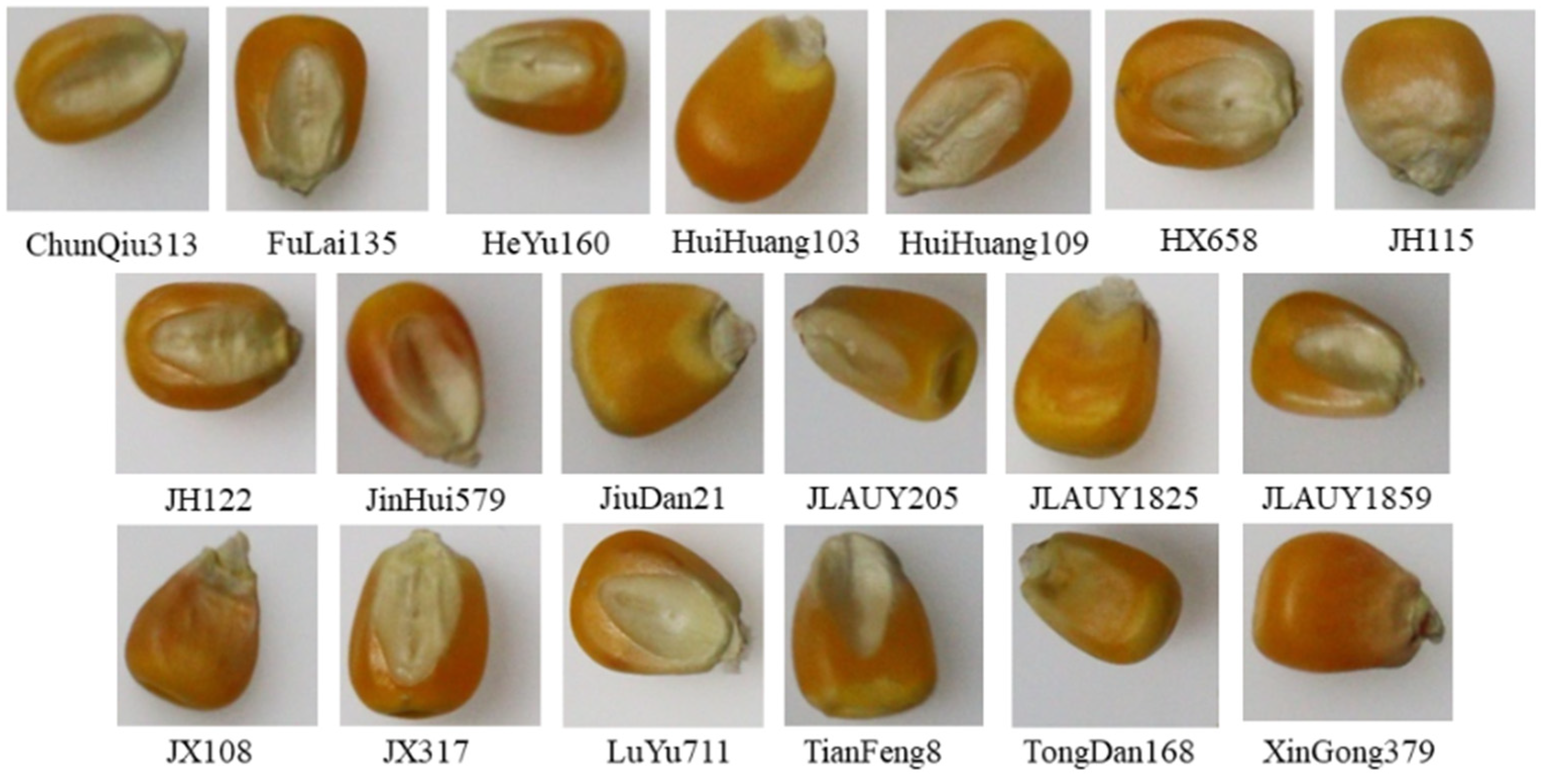
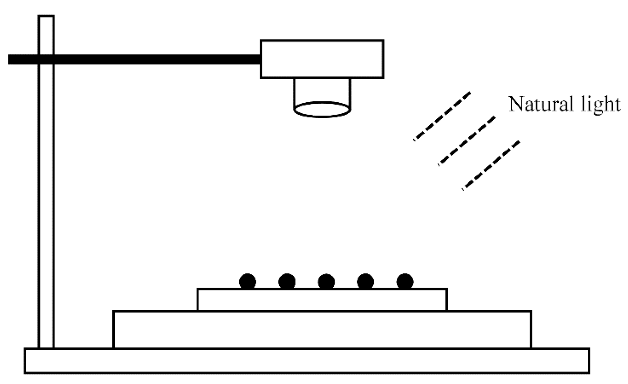
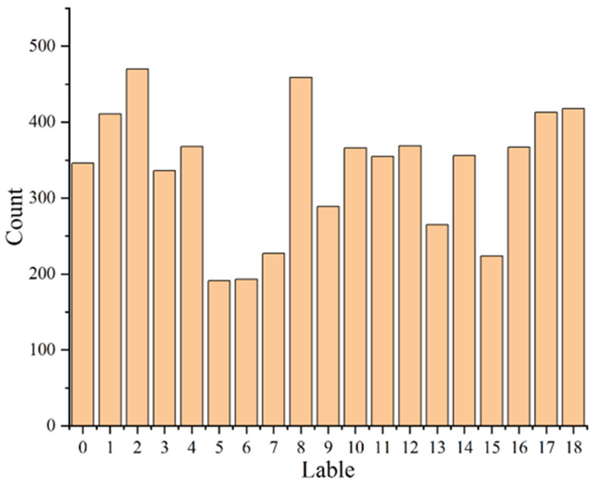
2.1.1. Data Source and Acquisition

In this study, 19 different maize seeds were selected, including ChunQiu313, FuLai135, HeYu160, HuiHuang103, HuiHuang109, HX658, JH115, JH122, JinHui579, JiuDan21, JLAUY205, JLAUY1825, JLAUY1859, JX108, JX317, LuYu711, TianFeng8, TongDan168, XinGong379 (Figure 1). In the process of sample selection, seeds with plump grains and uniform shape were manually screened as experimental samples, and the varieties to which they belonged were identified by experts. Then the image acquisition work is carried out. To ensure the randomness of the data, the canon 70D camera is used to capture the corn seed image under the indoor natural light. The acquisition equipment is shown in Figure 2.

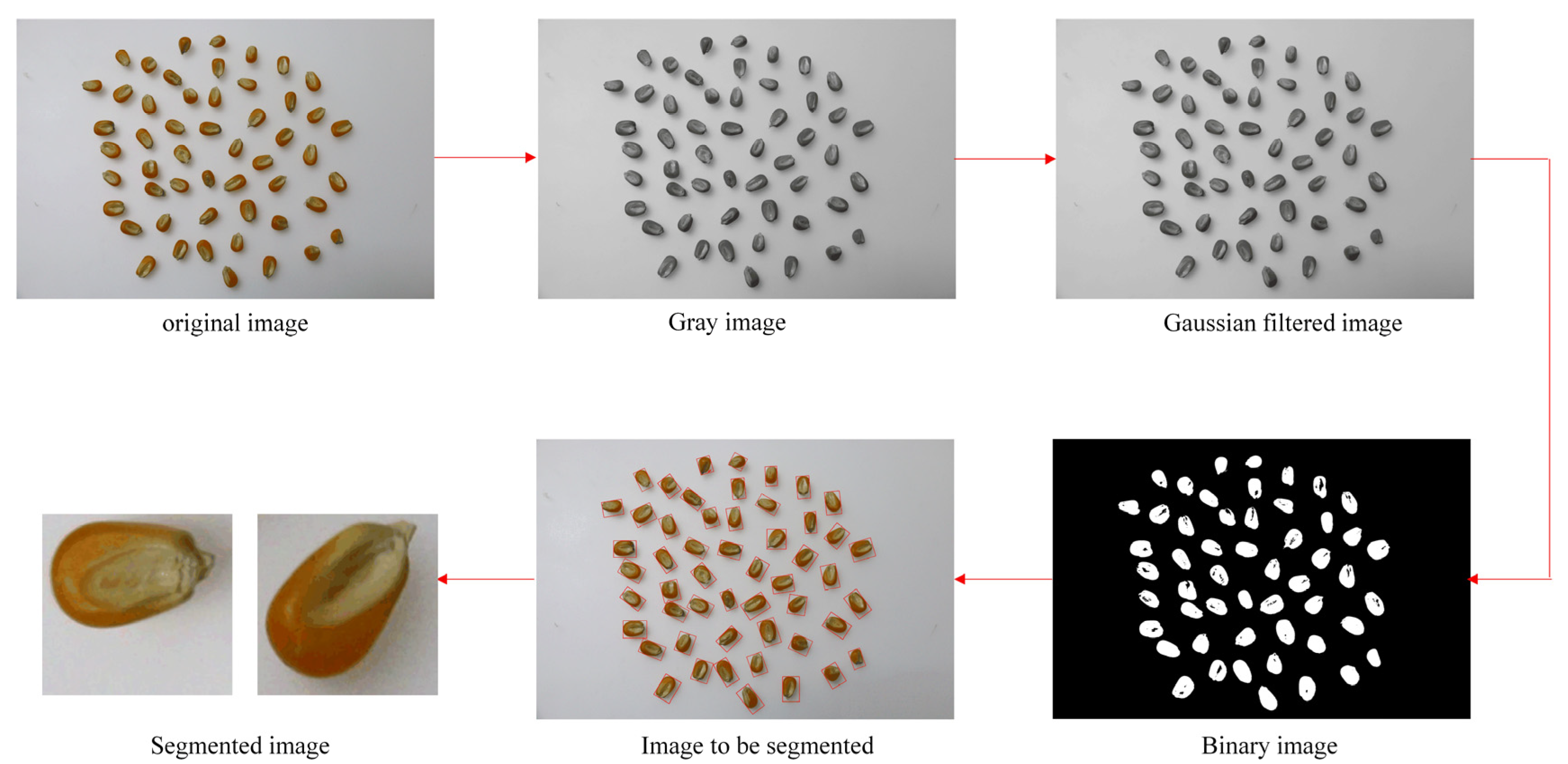
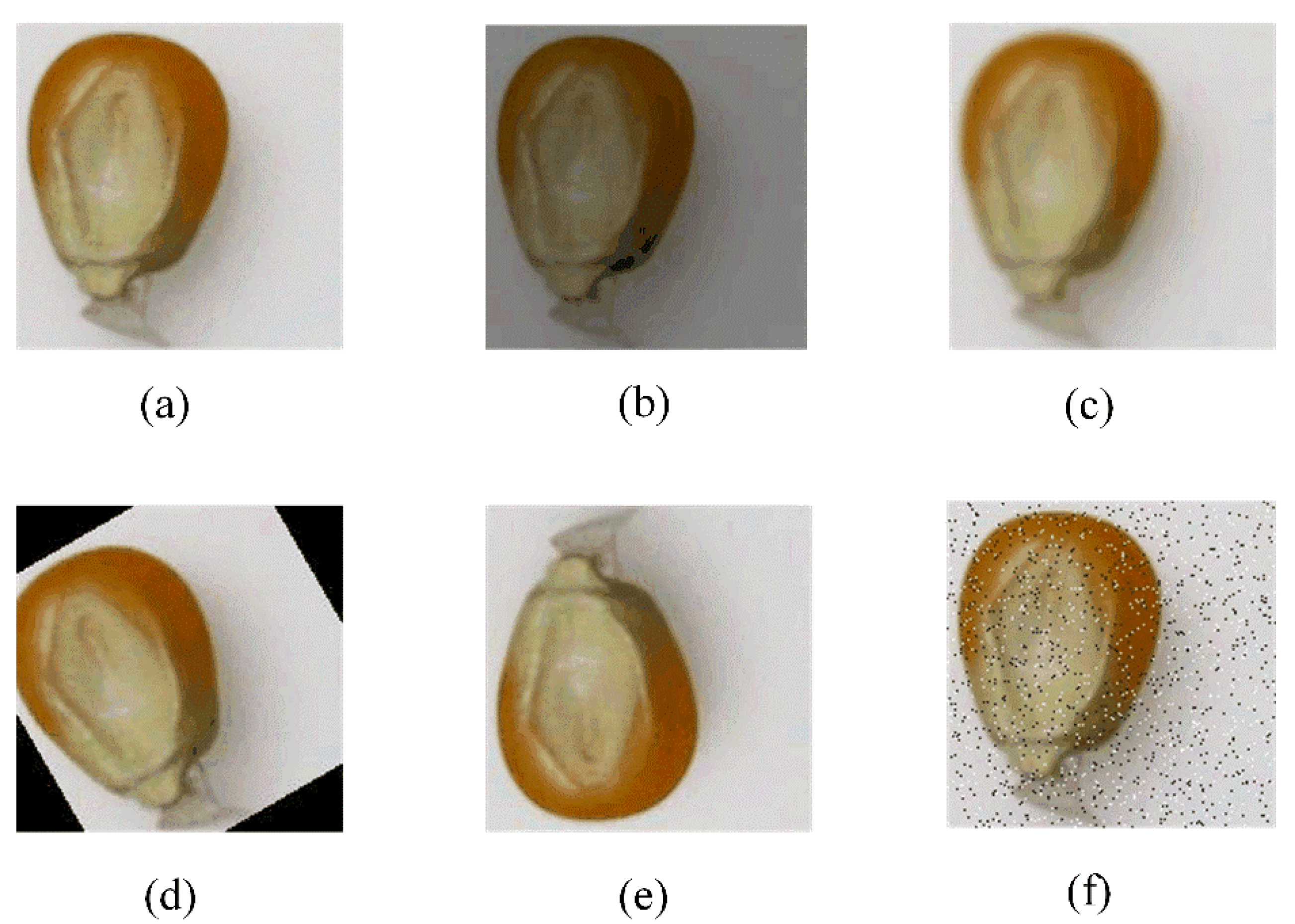
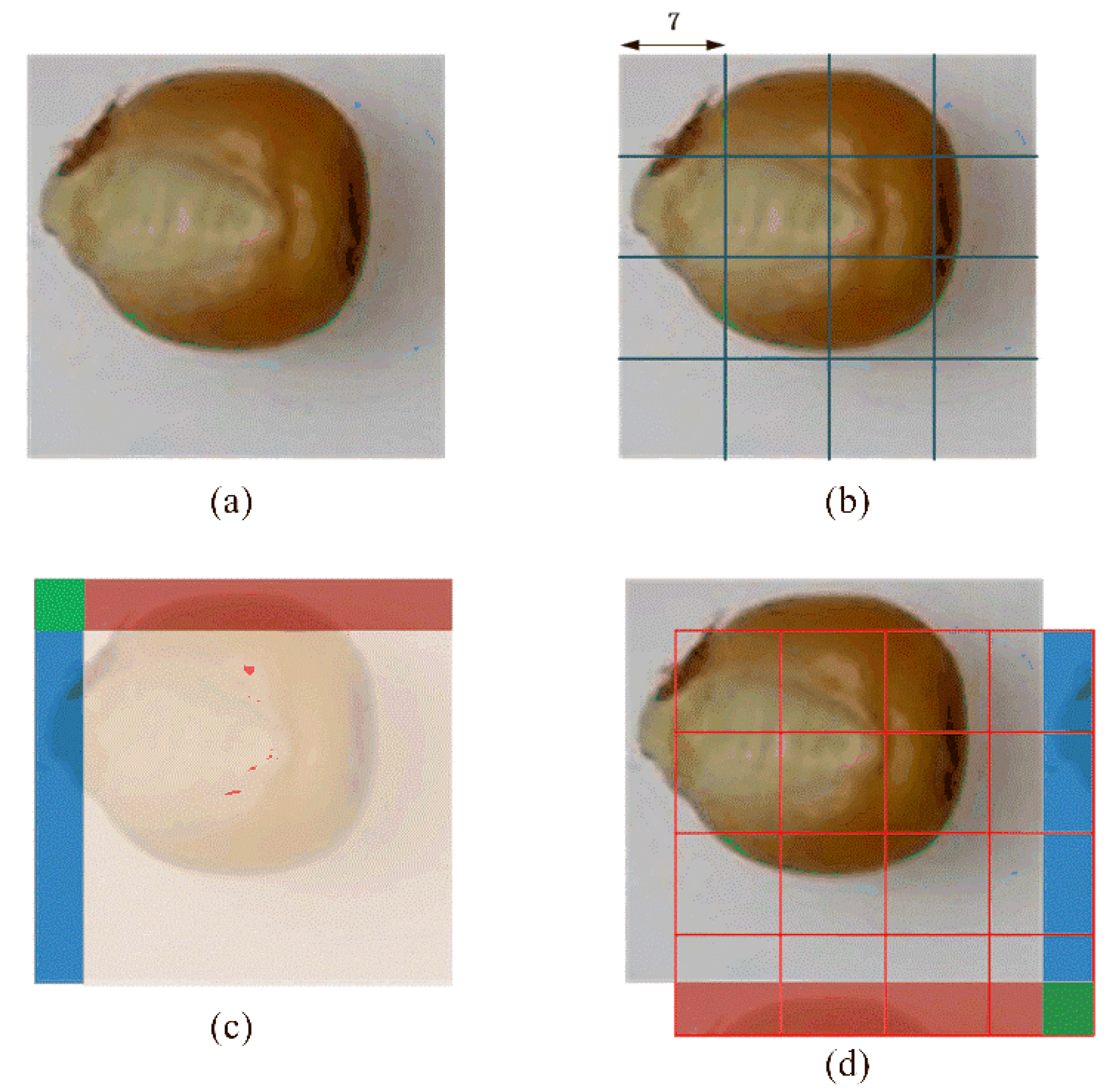
2.1.2. Image Preprocessing

The research on Maize Variety identification is the research on the authenticity and purity of maize seeds. Because the seed purity is composed of the authenticity of a single seed, the single seed identification method is used to identify the seed varieties [34]. The image containing multiple corn seeds needs to be cut (Figure 3). Firstly, the image is denoised by Gray processing and Gaussian filter [35], and then Thresholding [36]. The edge of the corn seed is obtained by the contour extraction algorithm, and then the coordinates of the center point and four vertices of the corn seed are obtained by the minimum circumscribed matrix method. Finally, the samples completely containing corn seeds were obtained by cutting, and a total of 6423 original images were obtained.

The sample distribution of the dataset is shown in Figure 4, where 0 is ChunQiu313, 1 is FuLai135, 2 is HeYu160, 3 is HuiHuang103, 4 is HuiHuang109, 5 is HX658, 6 is JH115, 7 is JH122, 8 is JinHui579, 9 is JiuDan21, 10 is JLAUY205, 11 is JLAUY1825, 12 is JLAUY1859, 13 is JX108, 14 is JX317, 15 is LuYu711, 16 is TianFeng8, 17 is TongDan168, and 18 is XinGong379.

It can be seen from Figure 4 that the total number of samples in the data set is insufficient and the distribution of various samples is uneven, which will affect the classification effect of the model [37,38]. To improve the generalization ability and robustness of the model, data enhancement methods such as vertical rotation, random brightness and salt and pepper noise are used to increase the number of data sets.

Figure 5 shows an example of image enhancement. Taking LuYu711 as an example, 224 original images are enhanced to 896 by random rotation and vertical flip, and then the images are expanded from 896 to 1563 by Gaussian blur, random brightness and salt and pepper noise.

As shown in

Table 1. Profile of samples.

Seed Category	Number of Original Samples	Number of Enhanced Samples	Label
ChunQiu313	346	1730	0
FuLai135	411	1631	1
HeYu160	470	1882	2
HuiHuang103	336	1680	3
HuiHuang109	368	1843	4
HX658	191	1329	5
JH115	193	1351	6
JH122	227	1580	7
JinHui579	459	1836	8
JiuDan21	289	1728	9
JLAUY205	366	1830	10
JLAUY1825	355	1774	11
JLAUY1859	369	1845	12
JX108	265	1847	13
JX317	356	1773	14
LuYu711	224	1563	15
TianFeng8	367	1835	16
TongDan168	413	1703	17
XinGong379	418	1740	18
Total	6423	32,500	/

, all kinds of samples in the expanded data set are basically balanced, with a total of 32,500. Then, 80% of the data set is randomly selected as the training set and 20% as the test set. This paper adopts the 5-fold cross verification method [39], that is, 20,790 pictures are extracted from the training set as training data and 5197 pictures as verification data each time, and the verification data is not repeated.

2.2. Model Building

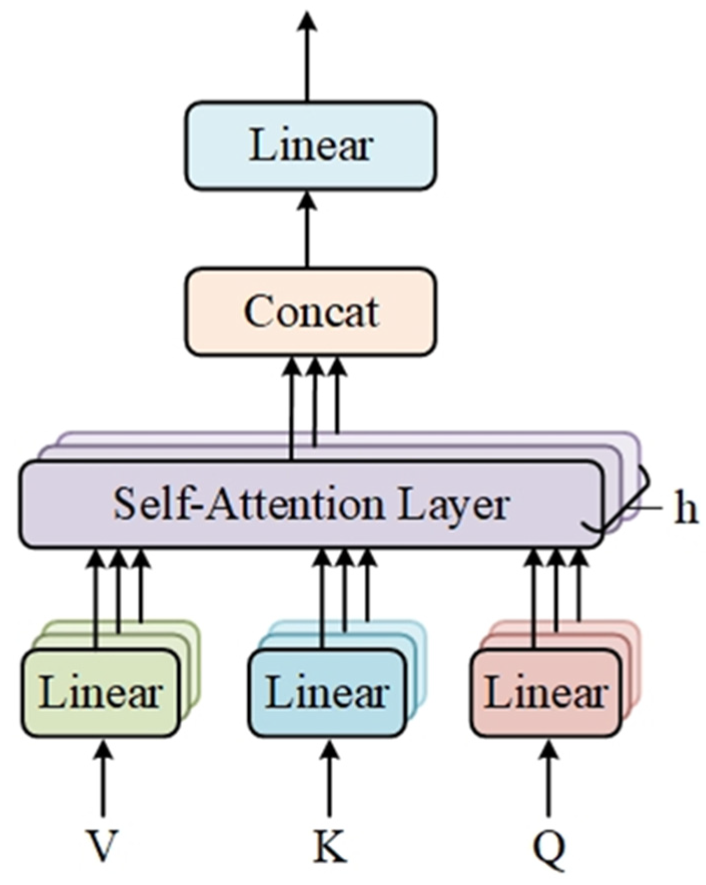
2.2.1. Transformer Model

The transformer model [40] was first applied in the field of natural language processing. It adopts encoder decoder architecture. Both are stacked by multi head attention layer, and feed forward network connection layer. Skip, connect and layer normalization layers are added behind each sub-layer. The core concept of the transformer is the multi head attention mechanism [41], which is connected by multiple self-attention. The structure is shown in Figure 6. The attention mechanism [42] actually wants the computer to imitate the human visual system and efficiently pay attention to the more critical information in the task goal. Self-attention first needs to set three trainable weight matrices Q, K and V; the input vector is multiplied by Q matrix, K matrix and V matrix to obtain the query vector, key vector and value vector, and then use the Scaled dot-product attention to calculate the attention weight,

$$self\_attention\left(Q,K,V\right)=Softmax\left(\frac{Q{K}^T}{\sqrt{d_k}}\right)V$$

(1)

where, Q, K and V represent query, key and value matrices, respectively; The vector dimension of each key is $d_k$,The dimension of the value is $d_v$. Finally, connect multiple self-attention mechanisms to form a multi head attention mechanism, and its calculation formula is as follows:

$$\begin{array}{c}MultiHead\left(Q,K,V\right)=Concat\left(hea{d}_1,\dots ,hea{d}_h\right)W^o\\ hea{d}_i=Attention\left(Q{W}_i^Q,K{W}_i^K,V{W}_i^V\right)\end{array}$$

(2)

where, $W^o$ is the weight matrix, $W_i^Q$, $W_i^K$, $W_i^V$ is the conversion matrix of Q, K and V, respectively; Concat means to merge the attention information of all headers.

With the continuous advancement of research, some scholars have migrated transformer technology to the field of computer vision [43,44]. Compared with convolutional neural network (CNN), the Transformer’s self-attention is not limited by local interaction, so that the model can not only be parallelized training, but also mine long-distance dependencies and extract more powerful features. Vision Transformer (ViT) [45,46] is the first work of transformer to replace standard convolution in machine vision. But the ViT model still has shortcomings such as being unable to model the spatial information of pictures, requiring large computing resources, and low learning efficiency. When the amount of data is not large enough, its advantages cannot be reflected.

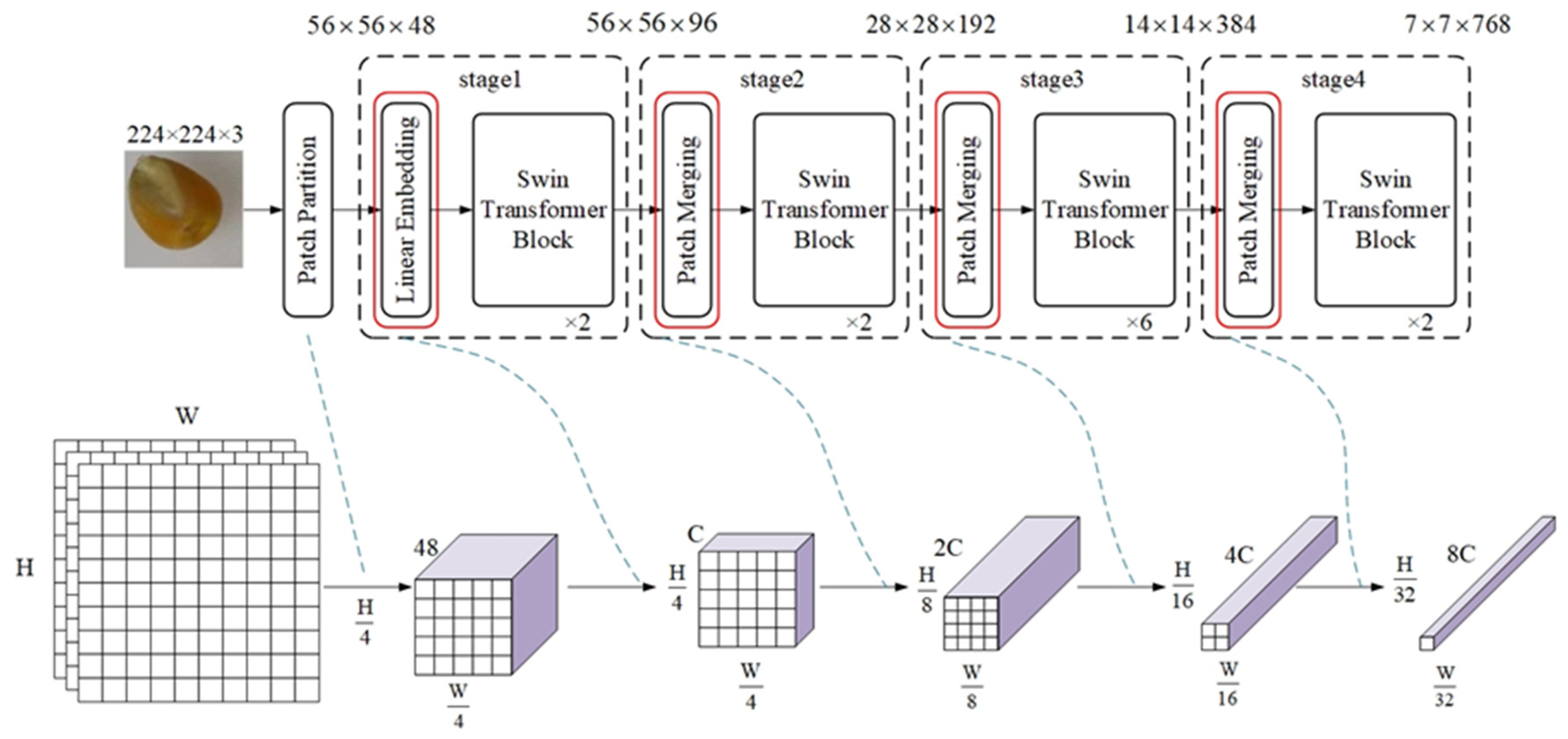
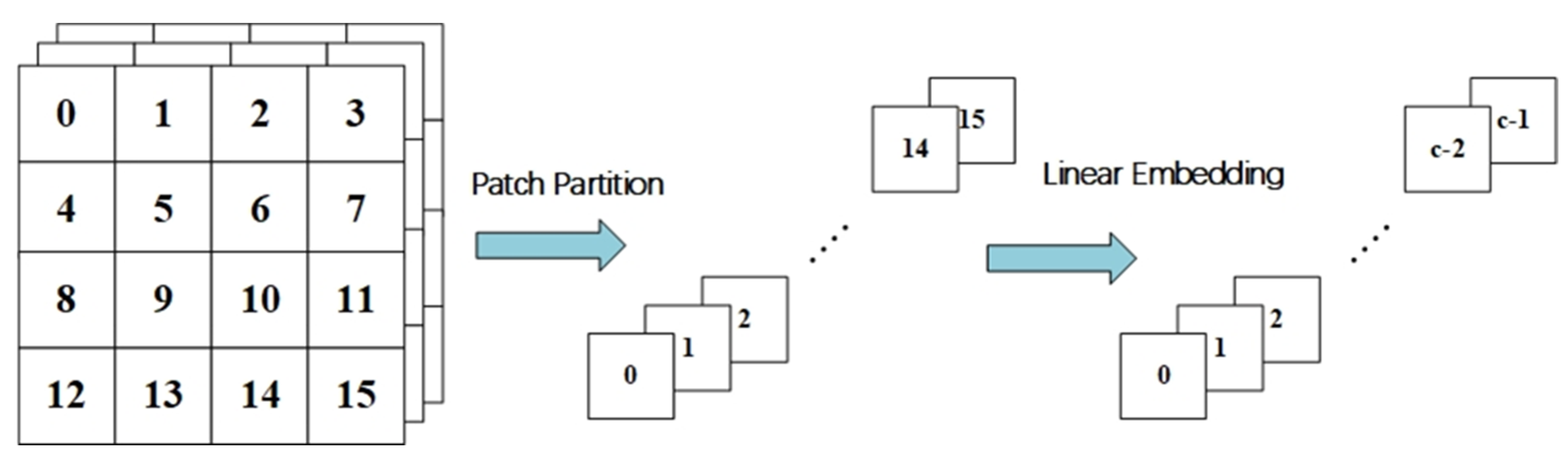
2.2.2. Swin Transformer Model

Aiming at some problems of Transformer model in CV field, Microsoft proposed an improved model-Swin Transformer model [47,48]. It adopts a hierarchical construction method, which not only has the advantages of CNN processing large-size images, but also has the advantages of using moving windows to establish long-range dependencies, which solves the problems of computational complexity and lack of information interaction between groups. The Swin-T network structure is shown in Figure 7.

Swin-T consists of four stages, and each stage reduces the resolution of the input feature map to expand the receptive field layer by layer. Similar to ViT, the image is first input into the Patch Partition module to divide the image into non-overlapping image blocks, each divided image block is regarded as a token, and the flattening operation is performed in the channel direction. The Linear Embedding module then uses linear variation to map it into a vector of dimension C (Figure 8). Each Swin Transformer module consists of two Blocks.

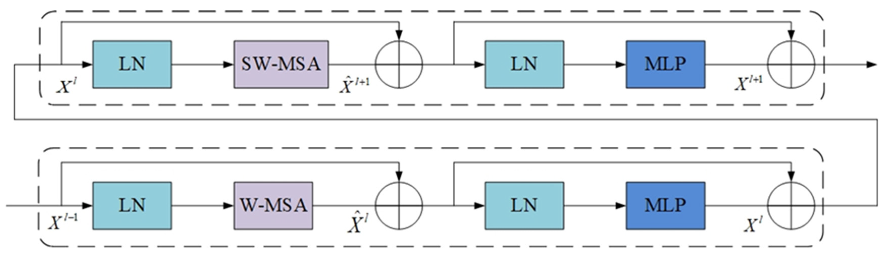
2.2.3. Swin Transformer Block

The core part of Swin-T is the Swin Transformer block, the detailed structure is shown in Figure 9. This module is a cascade of two multi-head attention modules, consisting of Windowed Multi-Head Self-Attention (W-MSA), Shifted Windowed Multi-Head Self-Attention (SW-MSA) and Multilayer Perceptron (MLP) [49].The LayerNorm layer is used before each MSA module and each MLP to make the training more stable and connected by residual after each module. Expressed as:

$$\begin{array}{c}{\widehat{X}}^l=W-MSA\left(\mathrm{LN}\right(X^{l-1}\left)\right)+X^{l-1}\\ X^l=MLP\left(LN\left({\widehat{X}}^l\right)\right)+{\widehat{X}}^l\\ {\widehat{X}}^{l+1}=SW-MSA\left(LN\left(X^l\right)\right)+X^l\\ X^{l+1}=MLP\left(LN\left({\widehat{X}}^{l+1}\right)\right)+{\widehat{X}}^{l+1}\end{array}$$

(3)

where, $X^l$ and ${\widehat{X}}^l$ denote the output features of the two self-attention modules and the MLP module in block L, respectively.

2.2.4. W-MSA Module and SW-MSA Module

Different from the multi-head self-attention used in the ViT model, the window multi-head self-attention (W-MSA) in the Swin-T model first divides the input image into non-overlapping windows, and then the pixels in each window can only be the inner product is performed with other pixels in the window to obtain information, so that the computational complexity of W-MSA is linearly related to the image size. In this way, the computational complexity of the network can be greatly reduced, thereby improving the computational efficiency of the network. The computational complexity of MSA and W-MSA are:

$$\begin{array}{c}\Omega (\mathrm{MSA})=4\mathrm{hw}{C}^2+2{(\mathrm{hw})}^{2}C\\ \Omega \left(W-MSA\right)=4hw{C}^2+2M^{2}hwC\end{array}$$

(4)

Among them, the former h × w has quadratic complexity, while the latter has linear complexity when M is fixed.

Although the computational complexity problem has been solved, the information interaction between windows can’t be carried out, resulting in the inability to obtain more globally accurate information, which will affect the accuracy of the network. To achieve information exchange between different windows, Shifted Window Multi-Head Self-Attention (SW-MSA) [50] is introduced. Each loop image is simultaneously shifted to the left and up by a certain window, then the cyan and red regions in Figure 10c are shifted to the right and below of the image, respectively. The SW-MSA mechanism can complete the pixel self-attention calculation of the offset window, thereby indirectly increasing the receptive field of the network and improving the efficiency of information utilization. The specific operation is shown in Figure 10.

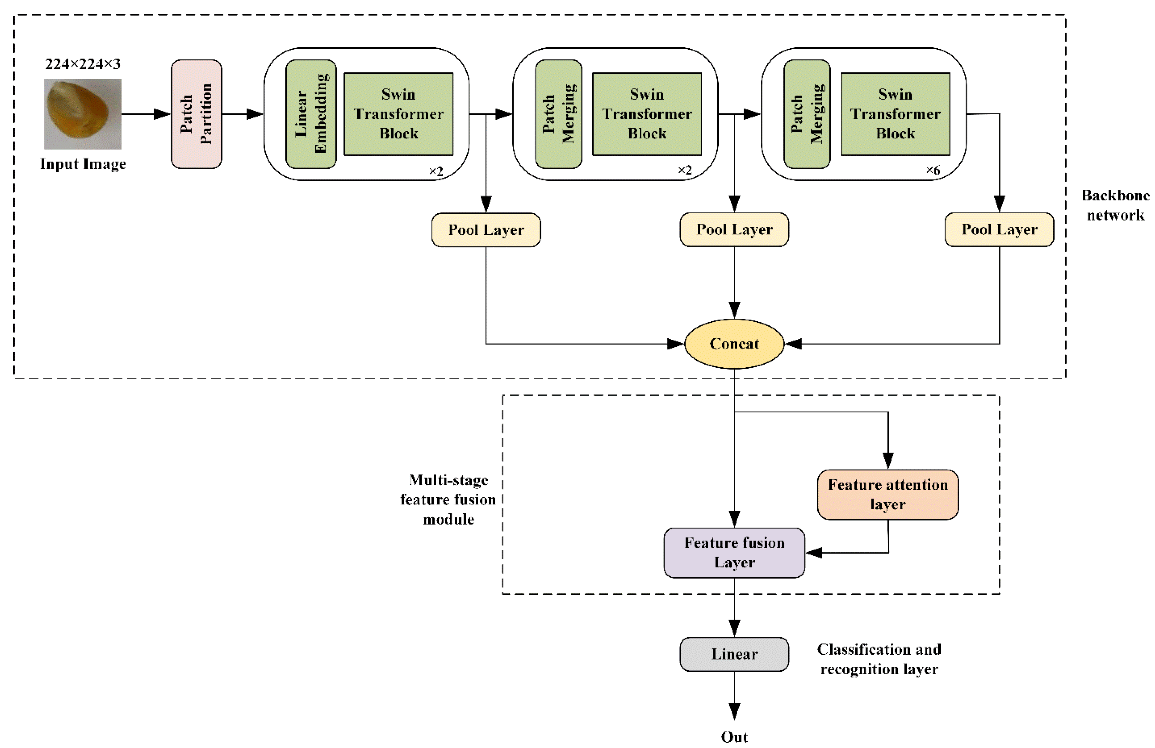
2.3. MFSwin-T Model Design

Swin-T can automatically learn from images and find discriminative and representative features and obtain final classification results by training the model. However, considering that the characters of corn seeds of different varieties are not obvious and difficult to distinguish, and there are differences between different varieties not only in shape and outline, but also in texture and details. The Swin-T model usually only utilizes the high-order features of the last stage, and the high-order features reflect more abstract semantic features, such as contour, shape and other features. The low-level semantic information is usually in the first few layers of the deep network, which can reflect the subtle changes in texture and color of seeds. Shallow networks contain more features and have the ability to extract key subtle features [51]. Although the shallow network has a strong ability to represent detailed information, its receptive field is small and lacks generalization of the overall seed image. In response to this problem, this paper considers the fusion of shallow network and deep network features, so as to learn a more comprehensive and effective feature representation, and extract corn seed information more completely [52]. Therefore, this paper establishes a network MFSwin-Transformer based on multi-scale feature fusion to classify 19 different varieties of maize seeds. The specific structure is shown in the Figure 11.

As can be seen from the figure, MFSwin-T model is composed of a backbone network, multi-stage feature fusion module and classification and recognition layer.

2.3.1. Backbone Network

The original Swin-T backbone network includes four stages. However, due to the increase in multi-head attention and the number of channels, it still occupies a large amount of computing resources and cannot meet the needs of real-time identification of corn seeds on resource-constrained devices. To avoid too many parameters, the increase in computational complexity leads to overfitting, so this paper cuts off stage 4 in the backbone network of the Swin-T model. First, input the image $I\in R^{C\times H\times W}$ into the network, and obtain the characteristics of each stage $F_1\in R^{C_1\times H_1\times W_1}$, where: C, H and W represent the input height, width and number of channels of the image, respectively; $C_1$, $H_1 \mathrm{and} W_1$ represent the height, width and number of channels of features at each stage, respectively. Specifically, the input image $I\in R^{224\times 224\times 3}$ is sent to the backbone network, the output size of stage1 is $F_1\in R^{56\times 56\times 96}$, the output of stage2 is $F_2\in R^{28\times 28\times 192}$, and the output of stage3 is $F_3\in R^{14\times 14\times 384}$. The Pool Layer is added after each stage, which consists of Linear, GELU, LayerNorm, and Average Pool. It mainly performs downsampling operation through the adaptive average pooling layer to unify the dimension of the feature vector, so that the dimensions of the features in different stages are the same. The unified dimensions are $F_{1,2,3}\in R^{1\times 1\times 384}$. Finally, the Concat method is used to splice the feature vectors obtained in different stages.

$$F_4=Concat\left(F_1,F_2,F_3\right)$$

(5)

Among them, $F_4$∈$R^{1\times 3\times 384}$ represents the dimension obtained by splicing the feature vectors of the three stages.

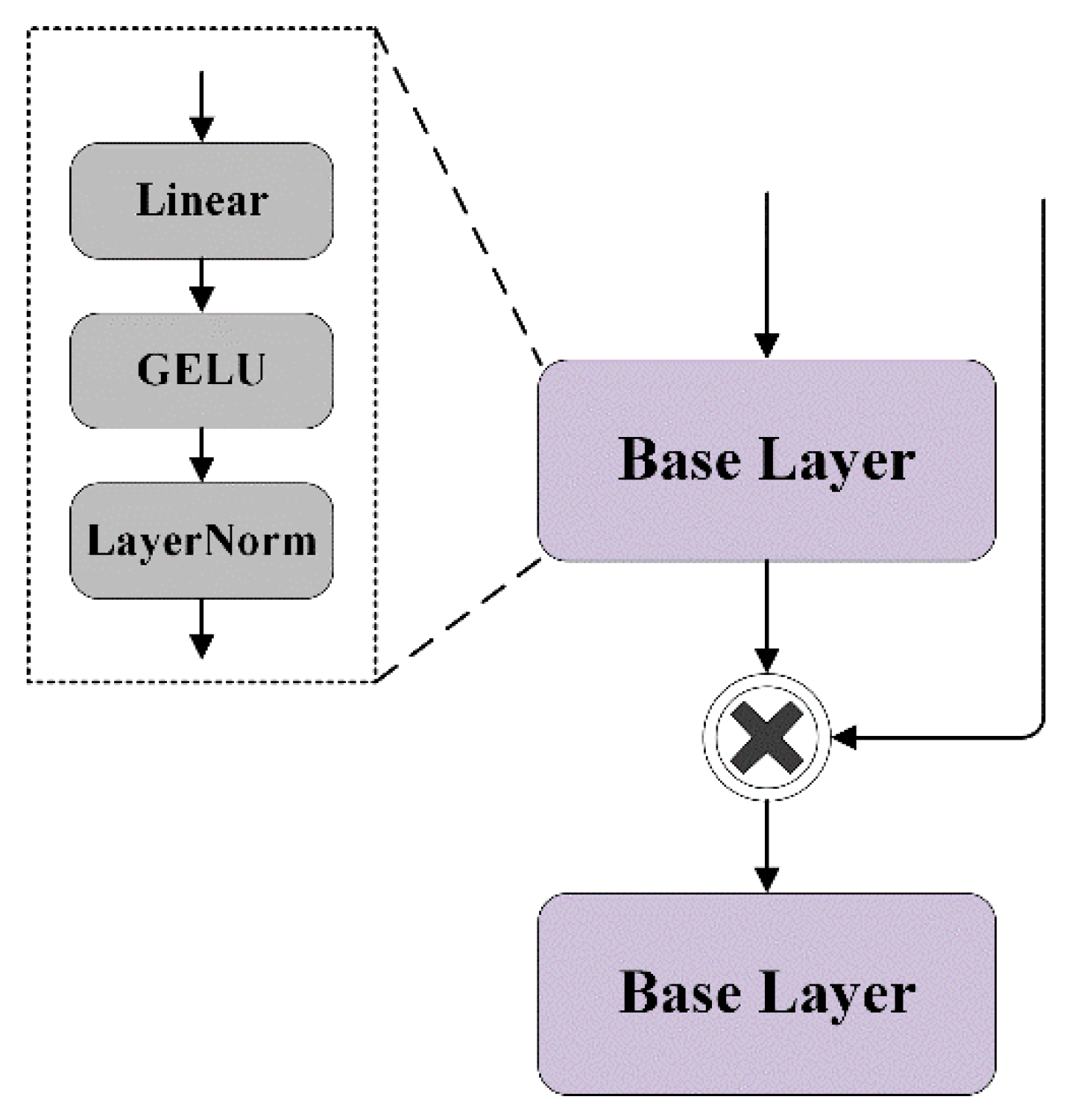
2.3.2. Multi-Stage Feature Fusion Module

The multi-stage feature fusion module takes the output of the backbone network feature extraction unit as input. To enable the model to selectively emphasize key features, this paper designs a feature attention layer, which consists of Linear and Softmax (Figure 12). The specific calculation is as follows:

$$w=Softmax\left(Linear\left(Mean\left(F_4\right)\right)\right)$$

(6)

Among them, w∈$R^{1\times 3\times 1}$, w represents the weight, Linear is a linear transformationMean ():$R^{1\times 3\times 384}$ -> $R^{1\times 1\times 384}$, represents the average operation of three eigenvectors. Softmax represents the normalized exponential function. Softmax’s formula is as follows:

$$Softmax\left(z_i\right)=\frac{\exp \left(z_i\right)}{{{\displaystyle \sum }}_j\exp \left(z_j\right)}$$

(7)

where z is a vector, $z_i$ and $z_j$ is one of the elements.

The stitched feature vectors are input into the feature attention layer, which gives different weights to the feature vectors in different stages to obtain $w_1,w_2,w_3$, Make the important features be assigned large weight to achieve enhancement, while other features are assigned small weight to achieve autonomous inhibition, so as to learn the key characteristics of different maize seed varieties. After the feature weight is obtained, it is passed into the feature fusion layer structure as shown in Figure 13, and the feature weight is multiplied by the feature vector element by element, and finally the multi-scale fusion feature $F\_final$ is obtained. The specific calculation is as follows:

$$F\_final=BL\left(Sum\left(\left(BL\left(F_4\right)\times w\right)\right)\right)$$

(8)

Among them, $F\_final$∈$R^{1\times 1\times 384}$, Sum ():$R^{1\times 3\times 384}$ -> $R^{1\times 1\times 384}$, BL is composed of Linear, GELU and LayerNorm.

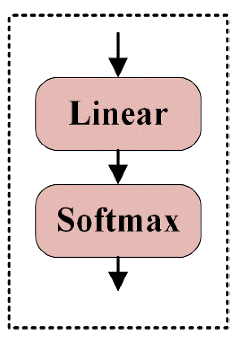
2.3.3. Classification and Recognition Layer

Finally, $F\_final$ is input into the SoftMax classifier for classification and recognition of 19 different varieties of corn seeds. Its specific calculation is as follows:

$$Out=Softmax\left(Linear\left(F\_final\right)\right)$$

(9)

Among them, $F\_final$∈$R^{1\times 19}$, represents the category of corn seeds.

3. Results

3.1. Experimental Environment and Hyperparameters

The classification model and comparative experiments proposed in this paper are all carried out in the Windows 10 operating environment, and the experimental models are implemented using the Pytorch deep learning framework. The specific experimental environment parameters are shown in

Table 2. Experimental environment configuration.

Accessories	Operating System	Development Framework	Development Language	CUDA	GPU	RAM
Parameter	Windows10	Pytorch1.11.0	Python3.8.3	11.4	GeForce RTX 3080	32 G

.

In order to train the best model, we conduct multiple pre-experiments using the original Swin transformer model, and the hyperparameters of the model are set as follows: The size of the input corn seed image is set to 224 × 224, and the learning rate is an important hyperparameter for deep learning. If the learning rate is set too small, the convergence of the network will be too slow and the training time will be prolonged; if the learning rate is set too large, it will lead to the shock cannot converge. Therefore, during the pre-experiment, the learning rate was divided into four groups, 0.1, 0.01, 0.001 and 0.0001, respectively, and the batch size was set to 8, 16, 32 and 64. Through the comparative experiment, the learning rate is finally set to 0.0001 and the batch size is set to 32. At the same time, in the pre-experiment process, it was found that the model can converge when the number of Epochs is less than 50, so the number of experimental training iterations Epochs is set to 50. At the same time, the optimizer of the network selects the Adaptive Moment (Adam), and selects the Cross-Entropy loss function. The hyperparameters of the specific model are shown in

Table 3. Parameters for model training.

Parameter.	Parameter Value
Epoch	50
Learning rate	0.0001
Batch-size	32
Optimizer	Adam

.

3.2. Evaluation Indicators

In the field of machine learning, confusion matrices are often used to compare the results of model classification in supervised learning. Each column of the matrix represents the predicted class, and each row represents the actual class. Taking the binary classification problem as an example, define the actual result as positive and the predicted result as positive, denoted as TP; if the actual result is negative, the predicted result is positive, denoted as FP; if the actual result is positive, the predicted result is negative, denoted as FN; The actual result is negative, the predicted result is negative, denoted as TN. The specific structure of the confusion matrix is shown in

Table 4. Confusion matrix of binary classification problem.

Confusion Matrix		Actual Results
		Positive	Negative
Forecast Results	Positive	TP	FP
	Negative	FN	TN

.

For the corn seed data set built in this paper, the confusion matrix is used to calculate the Accuracy, Precision, Recall and F1 score of each network as the index to evaluate the effect of the model on corn seed variety recognition. In a multi-class classification task, treat each breed individually as “positive” and all other breeds as “negative”. To measure the performance of the entire network, the average precision and recall of 19 different varieties were calculated. Usually, Precision and Recall are a pair of contradictory indicators, so this paper uses the F1 score to calculate the weighted average of Precision and Recall. The higher the F1 score, the higher the model prediction accuracy and the better the performance. The calculation process of each evaluation index is shown in

Table 5. Calculation formulas of each indicator.

Index	Formula	Significance
Accuracy	$Accuracy=\frac{TP+TN}{TP+TN+FP+FN}$	The number of correct predictions by the model, as a proportion of the total sample size
m-Precision	$m-Precision=\frac{TP}{TP+FP}$	Among the samples that the model predicts as positive, the model predicts the correct proportion of samples
Precision	$Precision=avg({\displaystyle {\displaystyle \sum }_{m=1}^{19}}m-Precision)$	Average accuracy of 19 varieties
m-Recall	$m-Recall=\frac{TP}{TP+FN}$	In the samples whose true value is positive, the model predicts the correct proportion of samples
Recall	$Recall={\displaystyle {\displaystyle \sum }_{m=1}^{19}}\left(m-Recall\right)$	Average recall rate of 19 varieties
F1-Score	$F1=2\times \frac{Recall\times Precision}{Recall+Precision}$	F1 score is the harmonic average of accuracy and recall

:

At the same time, in order to measure the performance of the network, the parameter memory requirements and FLOPs are also used as the evaluation indicators of the model. The parameter memory demand is determined by the number of parameters. On the premise of meeting the task requirements, the smaller the parameter memory, the less the consumption of computer memory resources and the higher the applicability. FLOPs refer to the number of floating point calculations, that is, the time complexity of the model. The lower the FLOPs, the less computation the model needs and the shorter the network execution time. FPS refers to the number of corn seed images processed per second, which can measure the recognition speed of the model. The larger the FPS, the faster the inference speed of the classification model.

3.3. Analysis of Experimental Results and Evaluation of Network Performance

3.3.1. Deep Feature Extraction Experiment

This experiment uses the Swin Transformer model. First, input the corn seed image into the network to get 7 × 7 deep features with 768 channels. Then, through the classification layer, the probability of 19 categories is predicted. The deep feature extraction experiment is the Baseline experiment in this paper. Finally, the average accuracy on the corn seed image dataset is 92.9%.

3.3.2. Multi-Scale Feature Fusion Experiment

This experiment extracts multi-scale features of corn seed images. To prevent overfitting due to too many parameters, we cut off Stage 4 in the Swin Transformer model. First, the corn seed image is input into the network, and the adaptive average pooling method is used to sample the features of the three stages, and the features are uniformly mapped to the channel dimension of 384. Then the features of the above three stages are spliced and fused on average to obtain multi-scale fusion features. Finally, the classifier is used for seed classification. The experimental accuracy is shown in the

Table 6. Indicators of ablation experiments.

Evaluation Indicators	Method
	Baseline	Multiscale Features	Multi-Scale Features + Feature Attention
Average Accuracy (%)	92.91	94.77	96.47
Average Precision (%)	93.36	94.26	96.53
Average Recall (%)	92.86	94.38	96.46
Average F1-Score (%)	93.00	94.27	96.47

. The average accuracy on the corn seed image dataset is 94.8%, which is 1.9% higher than that of the Baseline experiment. The experimental results show that the fusion of shallow network features and deep network features is effective, the shallow feature resolution is higher, and it has a strong ability to represent seed detail information.

3.3.3. Multi-Scale Feature Fusion Experiment with Feature Attention Layer

This experiment adds the feature attention layer based on the above experiment. Three feature weights can be obtained by passing the above average fused features through the attention layer, and then the feature weights are multiplied with the features of each stage to obtain the final multi-scale fused features. The experimental accuracy is shown in the Table 6. Compared with the 4.3.2 experiment, the accuracy is increased by 1.6%. The experimental results show that adding the feature attention layer can effectively integrate the features of different stages and improve the classification ability of the model for corn seed varieties.

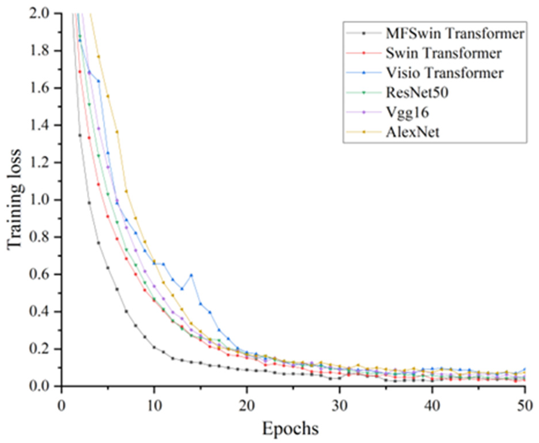
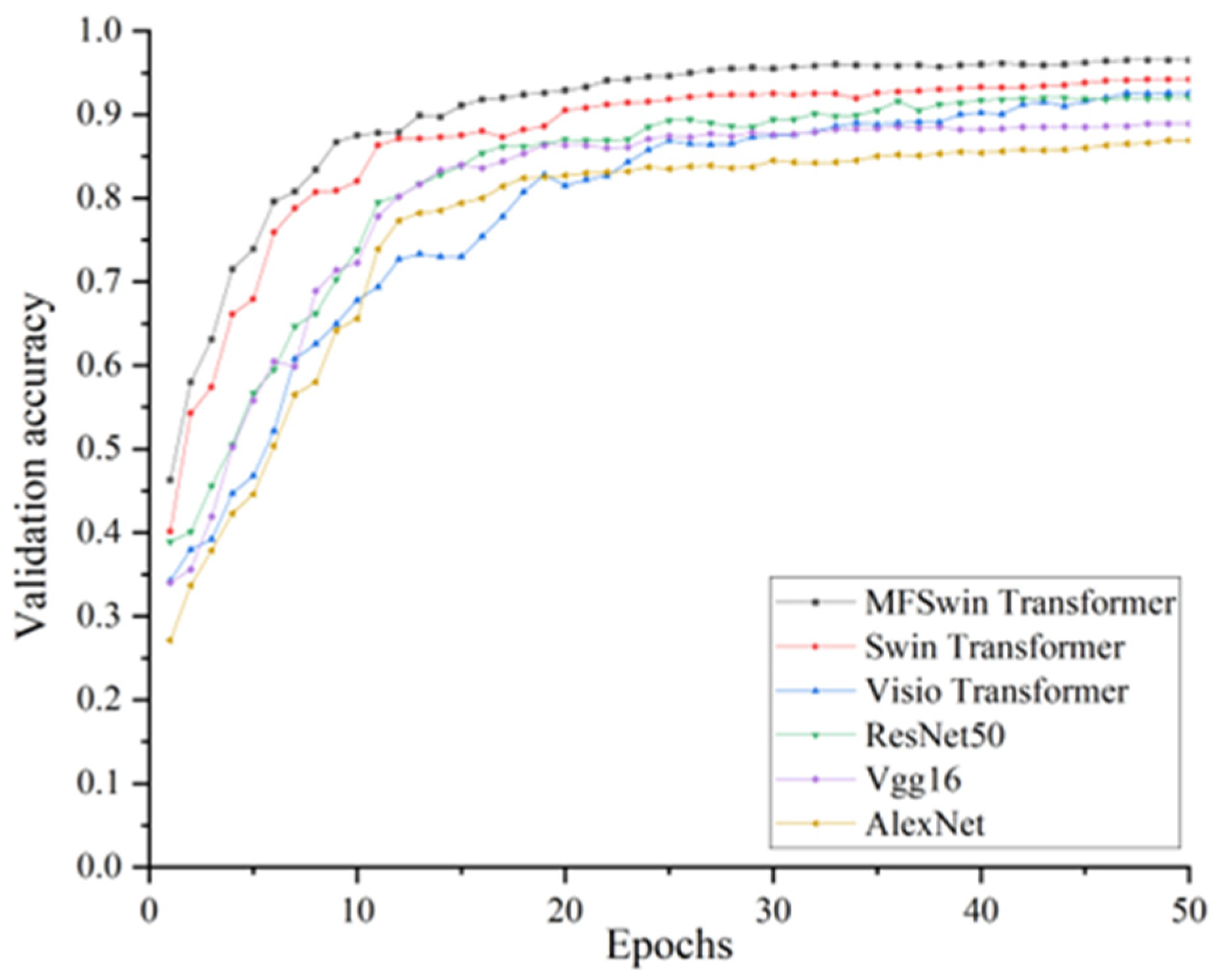
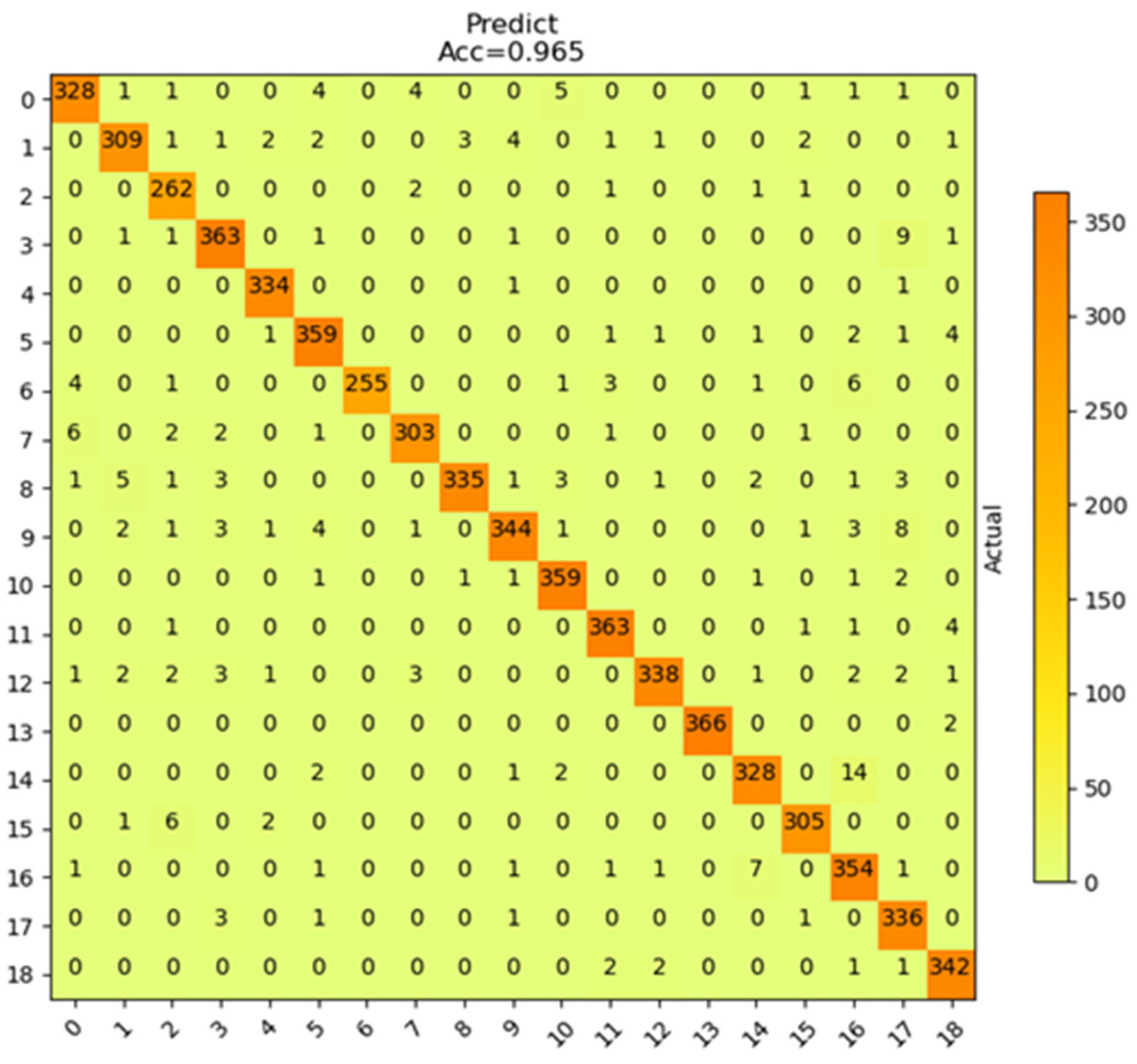
3.4. Comparative Experiment and Analysis

To verify the effectiveness and superiority of the improved model proposed in this paper, the MFSwin-Transformer model is compared with some representative convolutional neural networks [53,54,55] under the same dataset, experimental environment and the same network parameter configuration. Comparative experiments are carried out, including AlexNet [56,57,58], Vgg16 [59,60,61], ResNet50 [62,63,64], Visio-Transformer, Swin-Transformer models.

Table 7. Main parameters of classical convolutional neural network.

AlexNet	VGG16	ResNet50
Layer1: 11 × 11, 96; 3 × 3 Maxpool Layer2: 5 × 5, 256; 3 × 3 Maxpool Layer3: 3 × 3, 384 Layer4: 3 × 3, 384 Layer5: 3 × 3, 256; 3 × 3 Maxpool FC-1: 4096 FC-2: 4096 FC-3: 19 Classifier: Softmax	$\mathrm{Layer}1: \left[\begin{array}{c}3\times 3, 64\\ 3\times 3, 64\end{array}\right]$; 2 × 2 Maxpool $\mathrm{Layer}2: \left[\begin{array}{c}3\times 3, 128\\ 3\times 3, 128\end{array}\right]$; 2 × 2 Maxpool $\mathrm{Layer}3: \left[\begin{array}{c}3\times 3, 256\\ 3\times 3, 256\\ 3\times 3, 256\end{array}\right]$; 2 × 2 Maxpool $\mathrm{Layer}4: \left[\begin{array}{c}3\times 3, 512\\ 3\times 3, 512\\ 3\times 3, 512\end{array}\right]$; 2 × 2 Maxpool $\mathrm{Layer}5: \left[\begin{array}{c}3\times 3, 512\\ 3\times 3, 512\\ 3\times 3, 512\end{array}\right]$; 2 × 2 Maxpool FC-1: 4096 FC-2: 4096 FC-3: 19 Classifier: Softmax	Layer1: 7 × 7, 64; 3 × 3 Maxpool $\mathrm{Layer}2: \left[\begin{array}{c}1\times 1, 64\\ 3\times 3, 64\\ 1\times 1, 256\end{array}\right]\times 3$ $\mathrm{Layer}3: \left[\begin{array}{c}1\times 1, 128\\ 3\times 3, 128\\ 1\times 1, 512\end{array}\right]\times 4$ $\mathrm{Layer}4: \left[\begin{array}{c}1\times 1, 256\\ 3\times 3, 256\\ 1\times 1, 1024\end{array}\right]\times 6$ $\mathrm{Layer}5: \left[\begin{array}{c}1\times 1, 512\\ 3\times 3, 512\\ 1\times 1, 2048\end{array}\right]\times 3$ FC-1: 19 Classifier: Softmax

lists the main parameters of some comparison networks.

Figure 14 shows the relationship between the training loss value of each model and the iteration rounds. The loss curve represents the deviation between the predicted value and the real value of the network with the increase in iteration rounds. The smaller the loss value, the stronger the classification ability of the model and the smaller the probability of prediction error. It can be clearly seen from the figure that in the initial stage of training, the loss values of all networks are continuously decreasing, and eventually become stable without large fluctuations. Among them, the convergence speed of the MFSwin Transformer model is significantly better than other models. After the 13th epoch, the loss value of the MFSwin Transformer remained below 0.15, while the other models dropped below 0.15 after the 20th epoch. From the perspective of loss convergence, the training effect of the MFSwin Transformer model is optimal.

Figure 15 shows the relationship between the validation accuracy of each model and the number of iterations. The verification accuracy curve can describe the fluctuation of the recognition accuracy of the network as the number of iterations increases. As can be seen from the figure, the recognition accuracy of the MFSwin Transformer network has been continuously improved during the verification process. Compared with other comparative networks, the curve of the recognition accuracy of the MFSwin-T network is relatively smooth and stable, and there is no overfitting situation. The accuracy stabilizes above 90% after 13 epochs, while the other models only reach around 80% at the 13th epoch. It shows that the network has good recognition accuracy and generalization ability.

Table 8. Classification and comparison results of different networks.

Network	MFSwin-T	Swin-T	ViT	ResNet50	AlexNet	Vgg16
Average Accuracy (%)	96.47	92.91	92.00	91.29	88.75	85.95
Average Precision (%)	96.53	93.36	92.23	91.58	88.87	86.06
Average Recall (%)	96.46	92.86	92.06	91.31	88.82	86.06
Average F1-Score (%)	96.47	93.00	92.06	91.35	88.76	85.97

lists the classification performance of six different models, AlexNet, Vgg16, ResNet50, Swin Transformer, Visio Transformer, and MFSwin Transformer. Among them, the average accuracy, precision, recall, and F1-Score of the MFSwin-T model reached 96.47%, 96.54%, 96.46%, and 96.48%, respectively. It has better performance and higher accuracy than other models.

In addition, MFSwin-T has lower parameter memory and model complexity than other network models. As shown in

Table 9. Performance comparison results of different networks.

Network	FLOPs (G)	Params (M)	FPS
MFSwin-T	3.783	12.83	341.18
Swin-T	4.351	27.49	306.62
Vit	16.848	86.21	240.09
ResNet50	4.1095	23.55	304.65
AlexNet	0.711	57.08	365.76
Vgg16	15.480	134.34	294.80

, the computational complexity and parameter amount of the six models are shown. Under the same experimental environment and configuration, when the input corn seed image size is 224 × 224, the computational complexity of the MFSwin-T model is 3.783 G, and the parameter memory is 12.83 M. This is a reduction of 0.568 G and 14.66 M, respectively, compared to the network before the improvement. Meanwhile, compared with other networks, MFSwin Transformer has lower computational complexity and number of model parameters, where Vgg16 and Vit models have more than five times the computational complexity and seven times the number of parameters. And the image processing speed of MFSwin Transformer is also advantageous among all comparison models. It can be seen that MFSwin-T not only has faster network performance, but also can more accurately identify different varieties of corn seeds. These comparisons are enough to show the feasibility and superiority of the MFSwin-T model.

In order to evaluate the performance of the network more comprehensively, this paper draws a comparison and analysis diagram of the confusion matrix to reflect the actual recognition of each variety by the MFSwin Transformer network. As shown in Figure 16, due to the similar characteristics between seeds of different varieties, some varieties have large errors, such as JX317 and TianFeng8, which are prone to misclassification. However, it has higher accuracy and more advantages than manual recognition. But in general, the confusion matrix and classification results prove that the model proposed in this paper has good recognition ability for 19 kinds of corn seed categories, and the seeds of most varieties can be correctly recognized, indicating that the model can lay a good foundation for the recognition of highly similar seeds.

4. Discussion

In this work, we propose a non-destructive and efficient model for maize seed variety identification. First, we established a maize seed dataset with 19 varieties, and segmented the multi-seed images into images containing only single seeds by methods such as Gaussian filtering and contour extraction. In order to improve the generalization ability of the model, the data is augmented. According to the characteristics of different maize seed varieties with small differences in characteristics and details that cannot be ignored, this paper designs a maize seed variety recognition model MFSwin Transformer based on feature attention and multi-scale feature fusion. The model has high recognition accuracy and less parameters and has strong practicability. Maize seed varieties have the characteristics of small inter-class differences and large intra-class differences. Although a deeper network can obtain the outline and shape of seeds, it is easy to ignore some detailed features. Therefore, feature attention and multi-scale feature fusion are introduced to combine deep features and shallow features, so that the model can extract richer seed features. At the same time, to avoid overfitting caused by too many parameters, we cut off stage 4 in the backbone network. It can be seen from the ablation experiments that the improved method designed in this paper can improve the classification accuracy of the model and reduce the number of parameters and computational complexity of the model. However, it can be seen from the confusion matrix of the MFSwin Transformer model that some varieties are still classified incorrectly, which also reflects the need to further improve the ability of the model to extract fine features, so that it can provide better performance and accuracy under highly similar seed datasets. Because only low-cost digital cameras are needed to collect images, this method can be widely used and popularized in smart agriculture.

By comparing the performance of different models, the model proposed in this paper is better than other classic network models in terms of performance and recognition effect. Using deep learning to automatically extract image features is not only more effective but also avoids complex feature extraction in traditional recognition methods. However, this study only considers the classification effect of corn seed samples in the same year, and corn seeds of different years will have certain errors in color. In the follow-up study, the effects of different years, climatic and environmental factors, and geographical factors on seed classification can be compared.

5. Conclusions

In this paper, a non-destructive identification method is proposed, which can automatically classify different varieties of corn seeds from images, thereby overcoming the issue of large errors and low efficiency from the traditional methods. The main contributions of this study are:

(1) Collect the image containing multiple corn seeds, denoise and segment the image by using Gray processing, Gaussian filter and minimum circumscribed matrix, and get the image containing only a single corn seed. Finally, a dataset of maize seeds containing 19 different varieties was constructed, containing a total of 32,500 images. (2) According to the highly similar characteristics of maize seeds among different varieties, this paper integrates the shallow and deep features, and proposes a neural network maize seed image classification model MFSwin transformer based on feature attention and multi-scale feature fusion. The models and methods proposed in this paper provide a new idea for seed classification. (3) For the maize seed variety identification task, the proposed model (MFSwin Transformer) in this paper achieves relatively high classification results, and its accuracy, recall, and F1-score are substantially improved compared with the original model Swin Transformer, with an average recognition accuracy of 96%. Meanwhile, the number of parameters is only half of the original model, and the computational complexity of the model has been reduced. These results demonstrate the advantages and certain potential of the method in seed classification, which can provide high-quality maize seeds for agricultural production.

However, there are still some problems in this method that need to be solved urgently. Through experiments, it is found that the classification ability of this model between highly similar seeds still needs to be improved. Future research will continue to optimize the model so that it can be provided in more complex data sets with higher accuracy, forming an online real-time identification system capable of identifying multiple similar seeds.

References

1. García-Lara, S.; Serna-Saldivar, S.O.J.C. Corn History and Culture. Corn 2019, 1–18. [Google Scholar] [CrossRef]
2. Aimin, C.; Jiugang, Z.; Hu, Z. Preliminary exploration on current situation and development of maize production in China. J. Agric. Sci. Technol. 2020, 22, 10. [Google Scholar]
3. Costa, C.J.; Meneghello, G.E.; Jorge, M.H. The importance of physiological quality of seeds for agriculture. Colloquim Agrar. 2021, 17, 102–119. [Google Scholar] [CrossRef]
4. Queiroz, T.; Valiguzski, A.; Braga, C. Evaluation of the physiological quality of seeds of traditional varieties of maize. Revista da Universidade Vale do Rio Verde 2019, 17, 20193215435. [Google Scholar]
5. Sun, J.; Zou, Y. Analysis on the Method of Corn Seed Purity Identification. Hans J. Agric. Sci. 2020, 10, 292–298. [Google Scholar]
6. TeKrony, D.M. Seeds: The delivery system for crop science. Crop Sci. 2006, 46, 2263–2269. [Google Scholar] [CrossRef]
7. Sundaram, R.; Naveenkumar, B.; Biradar, S. Identification of informative SSR markers capable of distinguishing hybrid rice parental lines and their utilization in seed purity assessment. Euphytica 2008, 163, 215–224. [Google Scholar] [CrossRef]
8. Ye-Yun, X.; Zhan, Z.; Yi-Ping, X. Identification and purity test of super hybrid rice with SSR molecular markers. Rice Sci. 2005, 12, 7. [Google Scholar]
9. Satturu, V.; Rani, D.; Gattu, S. DNA fingerprinting for identification of rice varieties and seed genetic purity assessment. Agric. Res. 2018, 7, 379–390. [Google Scholar] [CrossRef]
10. Pallavi, H.; Gowda, R.; Shadakshari, Y. Identification of SSR markers for hybridity and seed genetic purity testing in sunflower (Helianthus annuus L.). Helia 2011, 34, 59–66. [Google Scholar] [CrossRef] [Green Version]
11. Lu, B.; Dao, P.D.; Liu, J. Recent Advances of Hyperspectral Imaging Technology and Applications in Agriculture. Remote Sens. 2020, 12, 2659. [Google Scholar] [CrossRef]
12. Wang, C.; Liu, B.; Liu, L. A review of deep learning used in the hyperspectral image analysis for agriculture. Artif. Intell. Rev. 2021, 54, 5205–5253. [Google Scholar] [CrossRef]
13. ElMasry, G.; Mandour, N.; Al-Rejaie, S. Recent applications of multispectral imaging in seed phenotyping and quality monitoring—An overview. Sensors 2019, 19, 1090. [Google Scholar] [CrossRef] [PubMed] [Green Version]
14. Hong, W.; Kun, W.; Jing-zhu, W. Progress in Research on Rapid and Non-Destructive Detection of Seed Quality Based on Spectroscopy and Imaging Technology. Spectrosc. Spectr. Anal. 2021, 41, 52–59. [Google Scholar]
15. Wang, L.; Sun, D.; Pu, H. Application of Hyperspectral Imaging to Discriminate the Variety of Maize Seeds. Food Anal. Methods 2015, 9, 225–234. [Google Scholar] [CrossRef]
16. Xia, C.; Yang, S.; Huang, M. Maize seed classification using hyperspectral image coupled with multi-linear discriminant analysis. Infrared Phys. Technol. 2019, 103, 103077. [Google Scholar] [CrossRef]
17. Zhang, J.; Dai, L. Corn seed variety classification based on hyperspectral reflectance imaging and deep convolutional neural network. Food Meas. Charact. 2020, 15, 484–494. [Google Scholar] [CrossRef]
18. Wang, Y.; Liu, X.; Su, Q. Maize seeds varieties identification based on multi-object feature extraction and optimized neural network. Trans. Chin. Soc. Agric. Eng. 2010, 26, 199–204. [Google Scholar]
19. Kiratiratanapruk, K.; Sinthupinyo, W. Color and texture for corn seed classification by machine vision. In Proceedings of the 2011 International symposium on intelligent signal processing and communications systems (ISPACS), Chiang Mai, Thailand, 7–9 December 2011. [Google Scholar]
20. Kamilaris, A.; Prenafeta-Boldú, F.X. Deep learning in agriculture: A survey. Comput. Electron. Agric. 2018, 147, 70–90. [Google Scholar] [CrossRef] [Green Version]
21. Stevens, E.; Antiga, L.; Viehmann, T. Deep Learning with PyTorch; Manning Publications: Greenwich, CT, USA, 2020. [Google Scholar]
22. Wani, J.A.; Sharma, S.; Muzamil, M. Machine learning and deep learning based computational techniques in automatic agricultural diseases detection: Methodologies, applications, and challenges. Arch. Comput. Methods Eng. 2021, 29, 641–677. [Google Scholar] [CrossRef]
23. Rawat, W.; Wang, Z. Deep convolutional neural networks for image classification: A comprehensive review. Neural Comput. 2017, 29, 2352–2449. [Google Scholar] [CrossRef]
24. Jena, B.; Saxena, S.; Nayak, G.k. Artificial intelligence-based hybrid deep learning models for image classification: The first narrative review. Comput. Biol. Med. 2021, 137, 104803. [Google Scholar] [CrossRef] [PubMed]
25. Thenmozhi, K.; Reddy, U.S. Crop pest classification based on deep convolutional neural network and transfer learning. Comput. Electron. Agric. 2019, 164, 104906. [Google Scholar] [CrossRef]
26. Zhao, Z.-Q.; Zheng, P.; Xu, S. Object detection with deep learning: A review. IEEE Trans. Neural Netw. Learn. Syst. 2019, 30, 3212–3232. [Google Scholar] [CrossRef] [PubMed] [Green Version]
27. Chen, Y.; Wu, Z.; Zhao, B. Weed and corn seedling detection in field based on multi feature fusion and support vector machine. Sensors 2020, 21, 212. [Google Scholar] [CrossRef] [PubMed]
28. Hu, D.; Ma, C.; Tian, Z. Rice Weed detection method on YOLOv4 convolutional neural network. In Proceedings of the 2021 International Conference on Artificial Intelligence, Big Data and Algorithms (CAIBDA), Xi’an, China, 28–30 May 2021. [Google Scholar]
29. Yu, C.; Wang, J.; Peng, C. Bisenet: Bilateral segmentation network for real-time semantic segmentation. In Proceedings of the European Conference on Computer Vision (ECCV 2018), Munich, Germany, 8–14 September 2018; pp. 325–341. [Google Scholar]
30. Giménez-Gallego, J.; González-Teruel, J.; Jiménez-Buendía, M. Segmentation of multiple tree leaves pictures with natural backgrounds using deep learning for image-based agriculture applications. Appl. Sci. 2019, 10, 202. [Google Scholar] [CrossRef] [Green Version]
31. Su, D.; Kong, H.; Qiao, Y. Data augmentation for deep learning based semantic segmentation and crop-weed classification in agricultural robotics. Comput. Electron. Agric. 2021, 190, 106418. [Google Scholar] [CrossRef]
32. Gulzar, Y.; Hamid, Y.; Soomro, A.B. A Convolution Neural Network-Based Seed Classification System. Symmetry 2020, 12, 2018. [Google Scholar] [CrossRef]
33. Sabanci, K.; Aslan, M.F.; Ropelewska, E. A convolutional neural network-based comparative study for pepper seed classification: Analysis of selected deep features with support vector machine. J. Food Process Eng. 2022, 45, e13955. [Google Scholar] [CrossRef]
34. Hong, P.T.T.; Hai, T.T.T.; Hoang, V.T. Comparative study on vision based rice seed varieties identification. In Proceedings of the 2015 Seventh International Conference on Knowledge and Systems Engineering (KSE), Ho Chi Minh City, Vietnam, 8–10 October 2015. [Google Scholar]
35. Buades, A.; Coll, B.; Morel, J.-M. A review of image denoising algorithms, with a new one. Multiscale Model. Simul. 2005, 4, 490–530. [Google Scholar] [CrossRef]
36. Szostek, K.; Gronkowska-Serafin, J.; Piórkowski, A. Problems of corneal endothelial image binarization. Schedae Inform. 2011, 20, 211. [Google Scholar]
37. Buda, M.; Maki, A.; Mazurowski, M.A. A systematic study of the class imbalance problem in convolutional neural networks. Neural Netw. 2018, 106, 249–259. [Google Scholar] [CrossRef] [PubMed] [Green Version]
38. Wan, X.; Zhang, X.; Liu, L. An Improved VGG19 Transfer Learning Strip Steel Surface Defect Recognition Deep Neural Network Based on Few Samples and Imbalanced Datasets. Appl. Sci. 2021, 11, 2606. [Google Scholar] [CrossRef]
39. Lopez-del Rio, A.; Nonell-Canals, A.; Vidal, D. Evaluation of cross-validation strategies in sequence-based binding prediction using deep learning. J. Chem. Inf. Modeling 2019, 59, 1645–1657. [Google Scholar] [CrossRef] [Green Version]
40. Vaswani, A.; Shazeer, N.; Parmar, N. Attention is all you need. Adv. Neural Inf. Processing Syst. 2017, 30, 1–11. [Google Scholar]
41. Xi, C.; Lu, G.; Yan, J. Multimodal sentiment analysis based on multi-head attention mechanism. In Proceedings of the 4th International Conference on Machine Learning and Soft Computing, Haiphong City, Vietnam, 17–19 January 2020. [Google Scholar]
42. Niu, Z.; Zhong, G.; Yu, H. A review on the attention mechanism of deep learning. Neurocomputing 2021, 452, 48–62. [Google Scholar] [CrossRef]
43. Han, K.; Wang, Y.; Chen, H.; Chen, X.; Guo, J.; Liu, Z.; Tang, Y.; Xiao, A.; Xu, C.; Xu, Y.; et al. A survey on visual transformer. arXiv 2020, arXiv:2012.12556. [Google Scholar]
44. Khan, S.; Naseer, M.; Hayat, M. Transformers in vision: A survey. ACM Comput. Surv. 2022. [Google Scholar] [CrossRef]
45. Dosovitskiy, A.; Beyer, L.; Kolesnikov, A. An image is worth 16x16 words: Transformers for image recognition at scale. arXiv 2020, arXiv:2010.11929. [Google Scholar]
46. Naseer, M.M.; Ranasinghe, K.; Khan, S.H. Intriguing properties of vision transformers. Adv. Neural Inf. Processing Syst. 2021, 34, 23296–23308. [Google Scholar]
47. Liu, Z.; Lin, Y.; Cao, Y. Swin transformer: Hierarchical vision transformer using shifted windows. In Proceedings of the IEEE/CVF International Conference on Computer Vision, Montreal, QC, Canada, 10–17 October 2021. [Google Scholar]
48. Liu, Z.; Lin, Y.; Cao, Y. Video swin transformer. In Proceedings of the IEEE/CVF Conference on Computer Vision and Pattern Recognition, New Orleans, LA, USA, 19–23 June 2022. [Google Scholar]
49. Zheng, H.; Wang, G.; Li, X. Swin-MLP: A strawberry appearance quality identification method by Swin Transformer and multi-layer perceptron. J. Food Meas. Charact. 2022, 1–12. [Google Scholar] [CrossRef]
50. Xu, X.; Feng, Z.; Cao, C. An Improved Swin Transformer-Based Model for Remote Sensing Object Detection and Instance Segmentation. Remote Sens. 2021, 13, 4779. [Google Scholar] [CrossRef]
51. Jiang, W.; Meng, X.; Xi, J. Multilevel Attention and Multiscale Feature Fusion Network for Author Classification of Chinese Ink-Wash Paintings. Discret. Dyn. Nat. Soc. 2022, 2022, 1–10. [Google Scholar] [CrossRef]
52. Qu, Z.; Cao, C.; Liu, L. A deeply supervised convolutional neural network for pavement crack detection with multiscale feature fusion. IEEE Trans. Neural Networks Learn. Syst. 2021, 1–10. [Google Scholar] [CrossRef] [PubMed]
53. Gu, J.; Wang, Z.; Kuen, J. Recent advances in convolutional neural networks. Pattern Recognit. 2018, 77, 354–377. [Google Scholar] [CrossRef] [Green Version]
54. Albawi, S.; Mohammed, T.A.; Al-Zawi, S. Understanding of a convolutional neural network. In Proceedings of the 2017 International conference on engineering and technology (ICET), Antalya, Turkey, 21–23 August 2017. [Google Scholar]
55. Kamilaris, A.; Prenafeta-Boldú, F.X. A review of the use of convolutional neural networks in agriculture. J. Agric. Sci. 2018, 156, 312–322. [Google Scholar] [CrossRef] [Green Version]
56. Zhu, L.; Li, Z.; Li, C. High performance vegetable classification from images based on alexnet deep learning model. J. Agric. Biol. Eng. 2018, 11, 217–223. [Google Scholar] [CrossRef]
57. Wang, L.; Sun, J.; Wu, X. Identification of crop diseases using improved convolutional neural networks. IET Comput. Vis. 2020, 14, 538–545. [Google Scholar] [CrossRef]
58. Lv, M.; Zhou, G.; He, M. Maize leaf disease identification based on feature enhancement and DMS-robust alexnet. EEE Access 2020, 8, 57952–57966. [Google Scholar] [CrossRef]
59. Albashish, D.; Al-Sayyed, R.; Abdullah, A. Deep CNN model based on VGG16 for breast cancer classification. In Proceedings of the2021 International Conference on Information Technology (ICIT), Amman, Jordan, 14–15 July 2021. [Google Scholar]
60. Zhu, H.; Yang, L.; Fei, J. Recognition of carrot appearance quality based on deep feature and support vector machine. Comput. Electron. Agric. 2021, 186, 106185. [Google Scholar] [CrossRef]
61. Ishengoma, F.S.; Rai, I.A.; Said, R.N. Identification of maize leaves infected by fall armyworms using UAV-based imagery and convolutional neural networks. Comput. Electron. Agric. 2021, 184, 106124. [Google Scholar] [CrossRef]
62. Mukti, I.Z.; Biswas, D. Transfer learning based plant diseases detection using ResNet50. In Proceedings of the 2019 4th International Conference on Electrical Information and Communication Technology (EICT), Khulna, Bangladesh, 20–22 December 2019. [Google Scholar]
63. Gupta, K.; Rani, R.; Bahia, N.K. Plant-Seedling Classification Using Transfer Learning-Based Deep Convolutional Neural Networks. Int. J. Agric. Environ. Inf. Syst. 2020, 11, 25–40. [Google Scholar] [CrossRef]
64. Sethy, P.K.; Barpanda, N.K.; Rath, A.K. Deep feature based rice leaf disease identification using support vector machine. Comput. Electron. Agric. 2020, 175, 105527. [Google Scholar] [CrossRef]
Figure 1. Image of maize seed varieties.
Agronomy 12 01843 g001
Figure 2. Corn seed image acquisition system.
Agronomy 12 01843 g002
Figure 3. Corn seed image cutting processing.
Agronomy 12 01843 g003
Figure 4. Data distribution and labeling.
Agronomy 12 01843 g004
Figure 5. Image enhancement effect: (a) original image (b) Random brightness (c) Gaussian blur (d) Random rotation (e) Vertical rotation (f) Salt and pepper noise.
Agronomy 12 01843 g005
Figure 6. Structure of multi head attention mechanism.
Agronomy 12 01843 g006
Figure 7. Swin Transformer model structure diagram.
Agronomy 12 01843 g007
Figure 8. Patch Embedding module.
Agronomy 12 01843 g008
Figure 9. Swin Transformer module network structure.
Agronomy 12 01843 g009
Figure 10. (a) Input image (b) Window segmentation of input image through W-MSA (c) Operation of moving window (d) Different window segmentation methods through SW-MSA.
Agronomy 12 01843 g010
Figure 11. MFSwin- T network structure diagram.
Agronomy 12 01843 g011
Figure 12. Feature attention layer.
Agronomy 12 01843 g012
Figure 13. Feature fusion layer.
Agronomy 12 01843 g013
Figure 14. Relationship between model training loss and iteration rounds.
Agronomy 12 01843 g014
Figure 15. Relationship between model verification accuracy and iteration rounds.
Agronomy 12 01843 g015
Figure 16. MFSwin-T Confusion matrix.
Agronomy 12 01843 g016