A Dynamic Detection Method for Phenotyping Pods in a Soybean Population Based on an Improved YOLO-v5 Network

Abstract

Pod phenotypic traits are closely related to grain yield and quality. Pod phenotype detection in soybean populations in natural environments is important to soybean breeding, cultivation, and field management. For an accurate pod phenotype description, a dynamic detection method is proposed based on an improved YOLO-v5 network. First, two varieties were taken as research objects. A self-developed field soybean three-dimensional color image acquisition vehicle was used to obtain RGB and depth images of soybean pods in the field. Second, the red–green–blue (RGB) and depth images were registered using an edge feature point alignment metric to accurately distinguish complex environmental backgrounds and establish a red–green–blue-depth (RGB-D) dataset for model training. Third, an improved feature pyramid network and path aggregation network (FPN+PAN) structure and a channel attention atrous spatial pyramid pooling (CA-ASPP) module were introduced to improve the dim and small pod target detection. Finally, a soybean pod quantity compensation model was established by analyzing the influence of the number of individual plants in the soybean population on the detection precision to statistically correct the predicted pod quantity. In the experimental phase, we analyzed the impact of different datasets on the model and the performance of different models on the same dataset under the same test conditions. The test results showed that compared with network models trained on the RGB dataset, the recall and precision of models trained on the RGB-D dataset increased by approximately 32% and 25%, respectively. Compared with YOLO-v5s, the precision of the improved YOLO-v5 increased by approximately 6%, reaching 88.14% precision for pod quantity detection with 200 plants in the soybean population. After model compensation, the mean relative errors between the predicted and actual pod quantities were 2% to 3% for the two soybean varieties. Thus, the proposed method can provide rapid and massive detection for pod phenotyping in soybean populations and a theoretical basis and technical knowledge for soybean breeding, scientific cultivation, and field management.

1. Introduction

The pod phenotype is an important agronomic soybean trait [1]. As a leaf homologous organ [2], the pod is an essential factor in determining grain yield and quality of the grain [3,4]. The accurate and rapid acquisition of soybean pod physiological and ecological traits is of great significance for soybean breeding, yield estimation and field management [5]. Traditional crop phenotype acquisition methods are mainly measured manually, which has the disadvantages of subjective error, low efficiency, and high labor cost. In particular, it is difficult to analyze crop group phenotyping on a large scale.

In recent years, with the development of computer and machine vision technology, plant high-throughput phenotyping technology has become a hotspot in agricultural information engineering research [6]. Currently, phenotyping collection platforms are divided into indoor and field types depending on the operating environment. Indoor phenotyping collection is used for plants collected from a field or cultivated in a greenhouse. For example, an automated plant phenotyping system that consists of a digital camera and an automated platform can automatically collect and analyze sequential images of soybean plants [7]. For large-scale genetic and management studies to capture plant growth, a low-cost greenhouse-based high-throughput phenotyping platform has been built to collect growth-related image-derived phenotypes [8]. Through a combination of a rotated image scanning platform and a deep-learning-based computer vision pipeline, a cost-effective phenotyping platform was built to generate and analyze large datasets of maize ear and kernel phenotypes [9].

Indoor phenotyping collection platforms can precisely collect physiological traits of a single plant or organ to avoid shielding between plants, but they cannot replace field phenotyping collection for features in complex field environments. In addition, indoor phenotyping collection cannot reflect the characteristics of crop populations in the natural field environment. According to different carriers, the types of field phenotyping collection platforms include unmanned aerial vehicle (UAV) remote sensing [10], vehicle-mounted [11], and fixed positions in a field [12]. For example, multiple light detection and ranging sensors are fixed on the front of a high-clearance tractor to achieve collecting crop phenotyping with the tractor running in the field [13]. Shafiekhani et al. [14] developed a robotic architecture for plant phenotyping, which consists of an autonomous ground vehicle and a mobile observation tower. This platform can collect high-throughput plant phenotyping in the field. Herzig et al. [15] attached red–green–blue (RGB) and multispectral cameras to a UAV to collect vegetation indexes and various morphological traits of crops for yield prediction. These studies on crop phenotyping collection in the field have played an important role in the development of crop phenotyping technology, mainly focusing on canopy, vegetation cover and group growth traits. It is still difficult to achieve a detailed phenotyping collection in the field, such as soybean pods distributed from the bottom of the stems to the canopy during crop reproductive stages.

Recently, with the development of deep learning and digital image processing technology, target detection technology has been applied to crop canopies, key organs, diseases, and insect pests, such as soybean pod phenotyping detection [16], tomatoes [17], and strawberries [18]. Detection algorithms based on deep learning are mainly divided into two categories: one category includes two-stage algorithms, which are represented by the region-convolutional neural network (R-CNN) [19], faster R-CNN [20], and mask R-CNN [21,22], of which the operating speed is so slow that it is difficult to meet the real-time requirements for crop phenotyping detection. The other category includes single-stage algorithms, which are represented by the single shot multibox detector (SSD) [23], and the you only look once (YOLO) algorithm [24], which can meet the real-time requirements but have comparatively lower detection precision. In target detection tasks in agriculture, the YOLO series algorithms [25,26] play an important role in single-stage algorithms, which compromise between speed and precision. Guo et al. [27,28] used an improved YOLO-v4 algorithm by fusing the K-means algorithm and an improved attention mechanism to detect the number of soybean pods of a single plant. Li et al. [29] proposed an improved YOLO-v5 algorithm based on a shallow feature layer to overcome the field environment noise to meet the practical requirements of wheat ear detection and counting. Ren et al. [30] and Pathoumthong et al. [31] proposed an improved YOLO-v5 algorithm by introducing an attention mechanism, which adds a squeeze-and-excitation (SE) module to the backbone network for the detection of crop stomata.

Although the above algorithms have been optimized according to plant physical and ecological traits in the process of transferring general object detection to plant phenotyping detection, these methods, which were mainly for phenotyping detection of a single plant and its key organs in a laboratory, are inadequate for detecting small target features in complex field environments. Phenotypic detection for key organs, such as pods below the canopy of the soybean population, has some problems, such as the crisscrossing of multiple plants and the shelter of leaves and pods. At present, it is not systematic to detect the physiological phenotype of the soybean population growth process, especially due to the lack of automatic consecutive detection methods for pod phenotyping in soybean populations in the field. Therefore, we propose a dynamic detection method for phenotyping pods in a soybean population based on an improved YOLO-v5 network.

The remainder of the paper is organized as follows. Section 2 presents the proposed method for processing soybean pod images and the specification of the improved process. Section 3 presents the experiments and results. Section 4 offers a discussion of the proposed method. Section 5 concludes the paper.

2. Materials and Methods

To effectively detect the phenotypic traits of soybean pods in the field, the Longken 3401 and Heihe 43 soybean varieties were taken as research objects, and a dynamic detection method for phenotyping pods in soybean populations is proposed in this paper based on an improved YOLO-v5 network. In this study, depth cameras and a servo drive system were used to build a field soybean three-dimensional color image collection vehicle to obtain soybean pod images in the field. Based on mixed depthwise convolution (MixConv), the feature pyramid network and path aggregation network (FPN+PAN) of YOLO-v5 was optimized by applying a multilayer small size convolution kernel to each channel group in the MixConv. Through the fusion of red–green–blue (RGB) and depth images, the ability to distinguish foreground and background in soybean fields was improved to avoid interference from multiple plants. At the same time, a method for detecting the number of pods in the soybean population in the field was developed by introducing a compensation algorithm to improve the precision of the evaluation of the number of pods in the soybean population.

2.1. Experimental Materials and Data Acquisition

2.1.1. Experimental Materials

The test samples were cultivated in Jianshan Farm, north of Heilongjiang Province, China. The varieties for testing were Longken 3401 and Heihe 43, which are indeterminate and subindeterminate podding habit soybean strains, respectively. The cultivation of Longken 3401 requires approximately 108 days from emergence to maturity, and the active accumulated temperature of ≥10 °C is approximately 1900 °C. The plants were unbranched, with an average height of approximately 920 mm, and the pods were slightly curved, sickle-shaped, and brown at maturity. The cultivation of Heihe 43 requires approximately 115 days from emergence to maturity, and the active accumulated temperature of ≥10 °C is approximately 2150 °C. There were no branches on the plants, of which the average height was approximately 750 mm and the pods were long-shaped and gray at maturity. In this experiment, the testing varieties were planted in the middle of May every year at the farm experimental plot located at 125°38′ E longitude and 48°87′ N latitude.

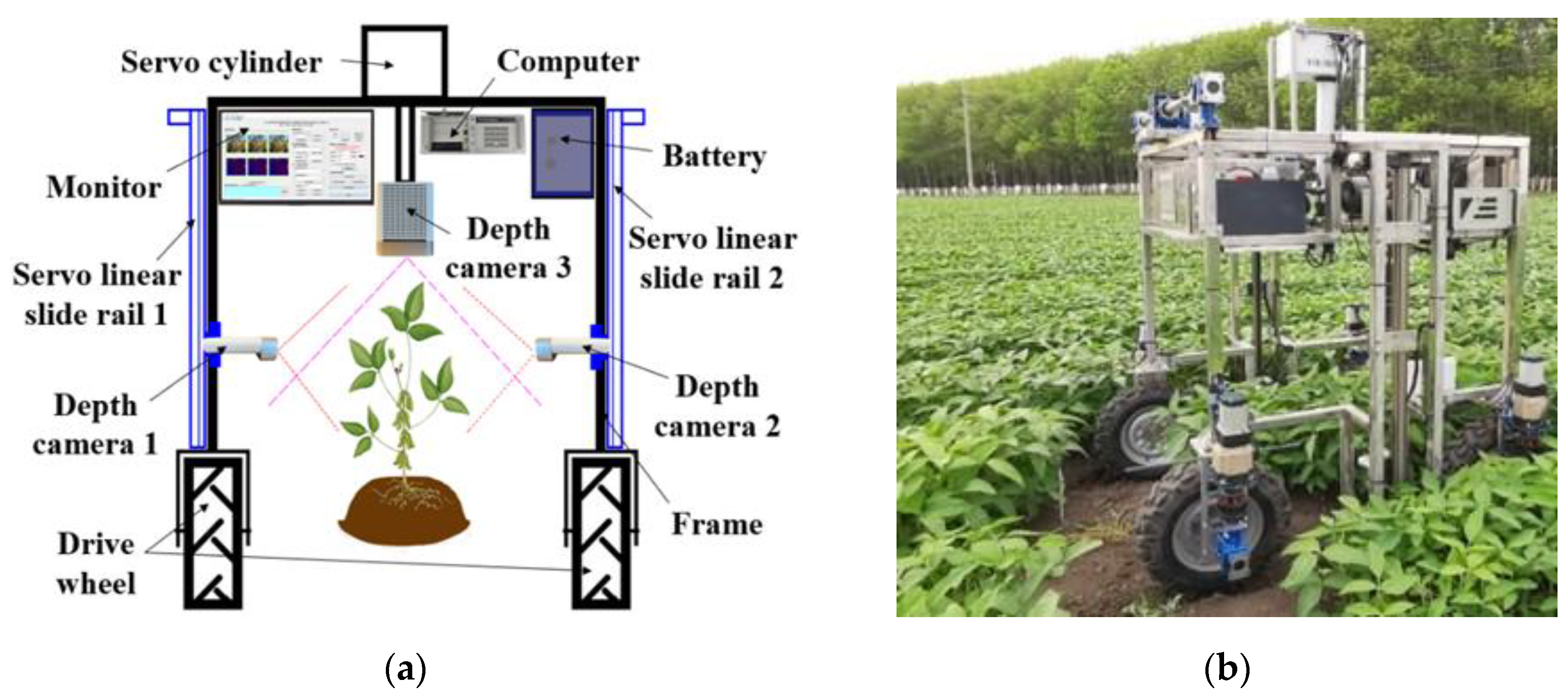
2.1.2. Construction of the Image Collection Platform

A field soybean three-dimensional color image acquisition vehicle was constructed based on an image acquisition, drive, and control system to dynamically collect digital image data of soybean pods in the field (as shown in Figure 1). The system consisted of three depth cameras, a graphic computer, a servo cylinder, two servo linear slide rails, four drive wheels, a homemade main frame with a height of 2100 mm, and a rechargeable battery. We used three Azure Kinect DK sensors (Microsoft Corp., Seattle, WA, USA) as the color and depth cameras, which were installed at the end of a servo cylinder fixed on the top of the frame and the servo linear slide rails fixed on two sides of the frame. The computer, monitor and battery were all installed in the upper corner of the frame to avoid interference with crops below. The top depth camera 3 was moved up and down over the crops by controlling the servo cylinder to locate the acquisition area as well as collect canopy phenotypic traits. The side depth cameras 1 and 2 moved up and down beside plants in the field via the automatic movement of the sliders on servo linear slide rails 1 and 2, as controlled by the computer control system, to achieve the pod phenotyping collection of entire soybean plants from the bottom of the stems to the canopy in the field. Each of the wheels supporting the frame was driven by a servo motor, and the power of all the electrical equipment was supplied by a battery on the vehicle. The dynamic detection for phenotyping of pods in soybean populations could be completed while the vehicle with depth cameras moved in a row of soybean plants.

2.1.3. Data Acquisition

The phenotypic traits of soybean pods from the full seed stage (R6) to the beginning maturity stage (R7) have an important influence on soybean yield and quality [32]. It is very important to accurately obtain the phenotypic traits of soybean pods in this growing period for target trait gene location and selection in soybean breeding. The image data of the test samples (as shown in Figure 2) were collected by using our image acquisition vehicle from the R6 to R7 stages of soybean growth from 2020 to 2022 to ensure data reliability. The soybean population in the experimental area was divided into 10 groups, each of which included varying numbers of plants from 20 to 200. Each testing group was planted at an interval of 500 mm, and there was no vegetation coverage on separation areas between groups. In the process of image acquisition, the depth camera, which was fixed on the top of the vehicle, was used to automatically locate the acquisition area to ensure that the entire group data were collected by detecting whether there was vegetation coverage in the area. The side cameras were used to collect the soybean pods of each row of plants in various groups. The collected depth image data were used to limit the distance from the targets to the image sensor to reduce the interference of complex backgrounds and improve the ability to distinguish the foreground and background in soybean fields.

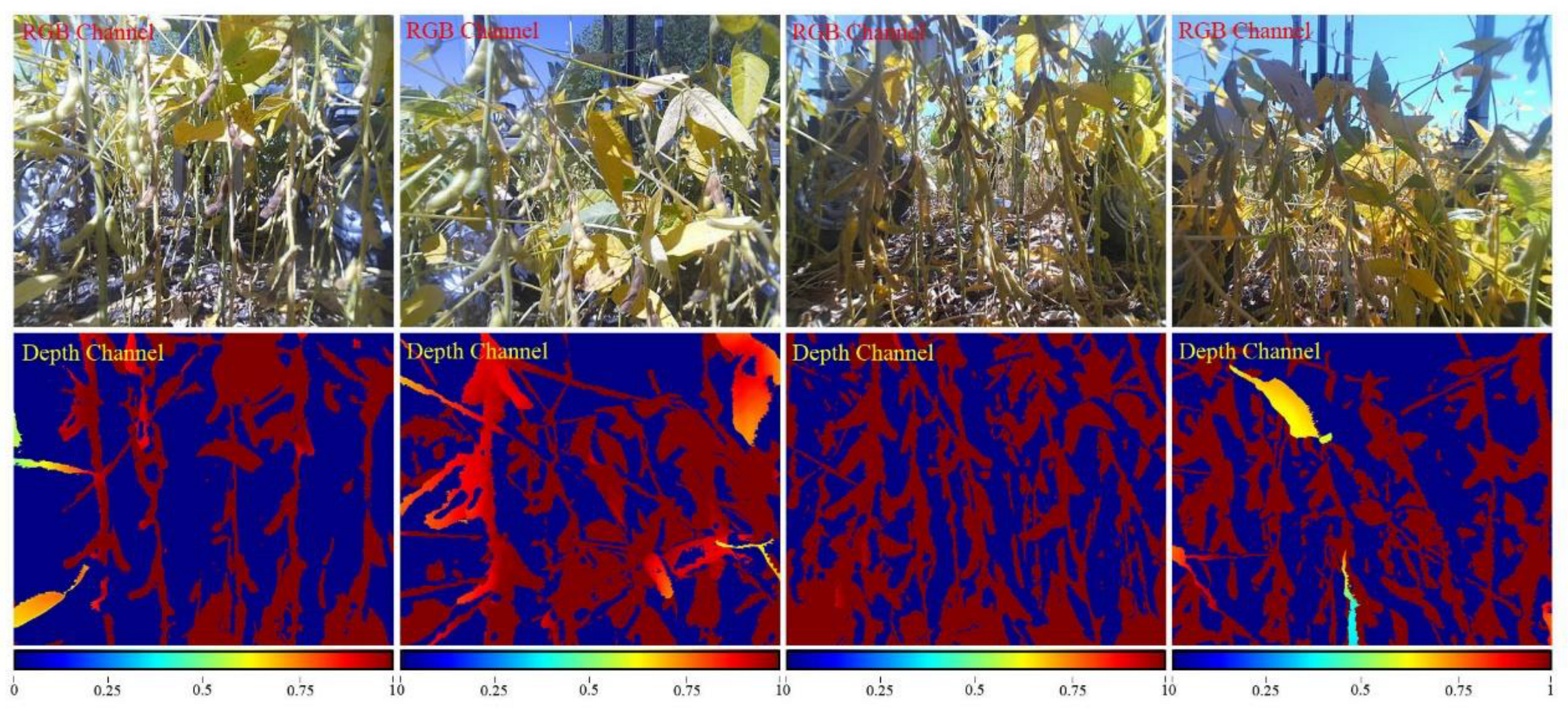
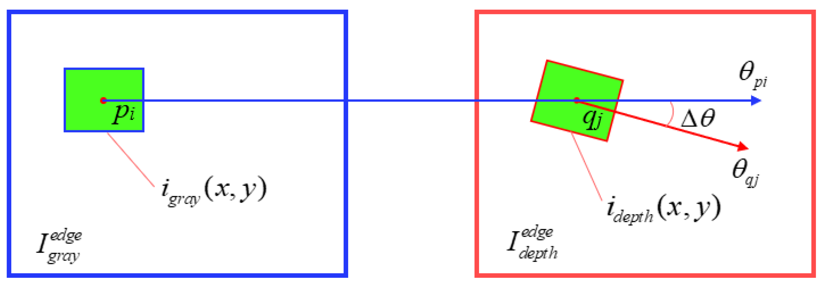
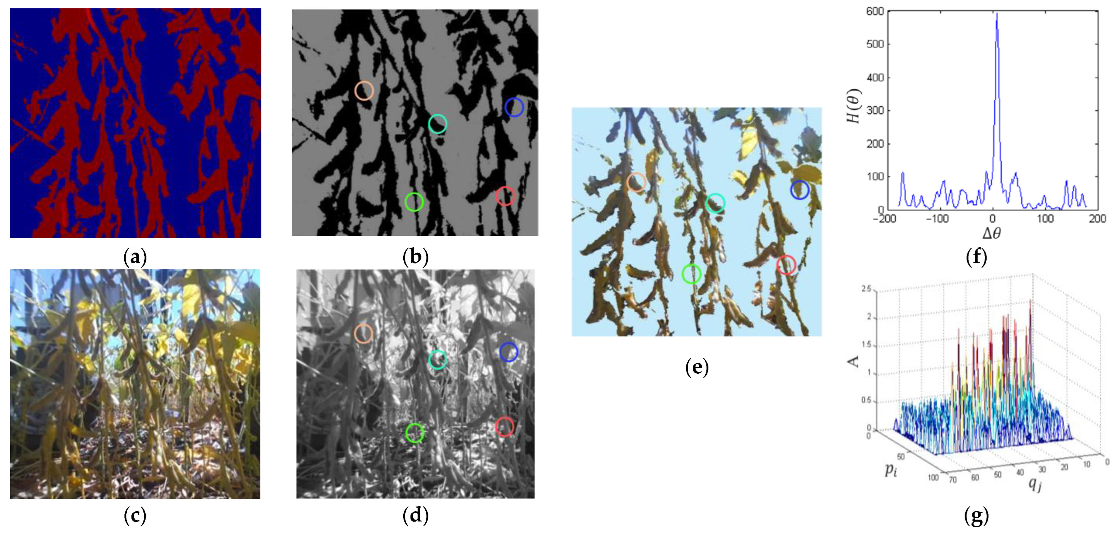
2.2. Data Preprocessing

Based on the previously established data collection method, we obtained 3500 RGB images and a corresponding number of depth images. To accurately remove the complex background area in RGB images through depth image data and retain the effective target area, feature matching based on edge shape information was used to fuse each RGB image and corresponding depth image because they had significantly similar graphic edge features. We used a wavelet multiscale edge detecting algorithm [33] to extract edge images and feature points from two images to be registered, determined the rotation angle between the two images based on the angle histogram of feature point pairs, and then matched the feature points of the two images using an edge feature point alignment metric.

The feature point sets extracted from $I_{gray}\left(x,y\right)$ and $I_{depth}\left(x,y\right)$ of the images to be registered were set to $P_{gray}=\{p_i|p_i={\left(p_x^i,p_y^i\right)}^T,i=1,2,\cdots ,N\}$ and $P_{depth}=\{q_j|q_j={\left(q_x^j,q_y^j\right)}^T,i=1,2,\cdots ,N\}$, then any feature point pair was $\left(p_i,q_j\right)$, $i,j=1,2,\cdots ,N$. ${\theta }_{pi}$ and ${\theta }_{qj}$ were the vector directions of $p_i$ and $q_j$, respectively; then, $H\left(\theta \right)$ in the angle histogram of feature point pairs indicates the number of corresponding feature point pairs $\left\{p_i\iff q_j\right\}$ in $P_{gray}$ and $P_{depth}$ when the angle differentials are $\Delta \theta$. Hence, if the value of $H\left(\theta \right)$ is maximum at $\Delta \theta =\overline{\theta }$, the rotation angle is $\overline{\theta }$ between images $I_{gray}\left(x,y\right)$ and $I_{depth}\left(x,y\right)$.

We supposed that $i_{gray}\left(x,y\right)$ and $i_{depth}\left(x,y\right)$ corresponded to sub feature images that were extracted from edge images $I_{gray}^{edge}$ and $I_{depth}^{edge}$ (as shown in Figure 3), in which the extraction for the sub feature image $i_{depth}\left(x,y\right)$ was in relation to the estimated rotation angle $\overline{\theta }$.

The edge feature point alignment metric is defined as follows.

$$A\left(p_i,q_j,\overline{\theta }\right)=\frac{1}{\epsilon \left(i_{gray},i_{depth}\right)},$$

(1)

where:

$$\epsilon \left(i_{gray},i_{depth}\right)=\frac{{\overline{\sigma }}_{gray,depth}^2}{{\sigma }_{depth}^2}+\frac{{\overline{\sigma }}_{depth,gray}^2}{{\sigma }_{gray}^2},$$

(2)

$${\sigma }_{gray}^2=\frac{1}{M·N}{{\displaystyle \sum }}_{\left(x,y\right)}{\left(i_{gray}\left(x,y\right)-{\mu }_{gray}\right)}^2,$$

(3)

$${\sigma }_{depth}^2=\frac{1}{M·N}{{\displaystyle \sum }}_{\left(x,y\right)}{\left(i_{depth}\left(x,y\right)-{\mu }_{depth}\right)}^2,$$

(4)

$${\mu }_{gray}=\frac{1}{M·N}{{\displaystyle \sum }}_{\left(x,y\right)}{i}_{gray}\left(x,y\right),$$

(5)

$${\mu }_{depth}=\frac{1}{M·N}{{\displaystyle \sum }}_{\left(x,y\right)}{i}_{depth}\left(x,y\right),$$

(6)

where ${\sigma }_{gray}^2$ and ${\sigma }_{depth}^2$ are the variances of $i_{gray}\left(x,y\right)$ and $i_{depth}\left(x,y\right)$, respectively, and ${\overline{\sigma }}_{gray,depth}^2$ is the expected variance of the corresponding pixel gray value set of image $i_{depth}\left(x,y\right)$ relative to the gray value of $i_{gray}\left(x,y\right)$. Similarly, ${\overline{\sigma }}_{depth,gray}^2$ is the expected variance of the corresponding pixel gray value set of images $i_{gray}\left(x,y\right)$ relative to the gray value of $i_{depth}\left(x,y\right)$.

Equation (2) is a mutual variance that reflects the stability of the gray levels of the two images. It can be seen that the more similar the content of the two images is, the smaller their mutual variance is. The registration does not require a linear correlation between the gray levels of the two images, nor is it affected by the difference in the gray level properties of the two images. Figure 4 shows that the angle histogram of the feature point pairs has obvious peaks in a certain angle difference, while the number of corresponding points is few in other angle differences, so that the angle differences can be accurately obtained. Through the fusion of the RGB and depth images, we finally obtained soybean plant images with no background to reduce interference from overlapping plants during detection. The LABELIMG software was used to label the images into a visual object classes (VOC) dataset, including object position, anchor frame size and labels of different forms of pods.

The labels of pods with different morphologies are represented by numbers; that is, an empty pod was represented by 0, a pod with one seed was represented by 1, a pod with two seeds was represented by 2, a pod with three seeds was represented by 3, and a pod with four seeds was represented by 4. The classification of the different morphologies of pods is shown in Figure 5. The total number of all labeled pods is 28,725, in which the largest number was pods with three seeds, accounting for 44.67% of the total, followed by pods with two seeds, four seeds, one seed, and empty pods (as shown in Figure 6). There were no pods with five or more seeds in the testing samples.

To obtain a well-performing neural network model and improve model generalization ability, the original images were adjusted for brightness, horizontal flipping, and saturation, randomly cropped, scaled, and arranged. Then, we combined the enhanced data with the original data into a dataset with a total of 14,000 images. The flow of image data processing is shown in Figure 7.

2.3. Detection Algorithm Principle

Through research and analysis of the YOLO-v5 network model, to improve the detection capability for small targets in complex environments, we proposed an improved YOLO-v5 network model by introducing an improved FPN+PAN structure and channel attention atrous spatial pyramid pooling (CA-ASPP).

2.3.1. The YOLO-v5 Network Model

YOLO-v5 is the fifth version of the YOLO algorithm. According to the difference in network width and depth, YOLO-v5 is subdivided into YOLO-v5s, YOLO-v5m, and YOLO-v5l, in which YOLO-v5s is the version with the smallest network width and depth [34]. Other versions of YOLO-v5 are the result of widening and deepening the network according to a certain proportion based on YOLO-v5s [35]. Wang et al. used a YOLO-v5s model to detect apple fruitlets. The method achieved an 87.6% and 95.8% recall and accuracy for apple detection in orchards, respectively [36]. Since YOLO-v5s is small in size and requires low computing power, it can be deployed and applied with low configuration hardware equipment on field soybean image acquisition vehicles.

The basic idea of YOLO-v5 was to separate the augmented data of input images into S × S cells, and that each cell generates prediction boxes. The location of the prediction box was determined by the cell of the detected target center and the two adjacent cells through position regression. Additionally, the probability of whether the prediction box has a target and the probability that the target belongs to a certain category was calculated. For targets of different sizes, YOLO-v5 used three detection heads to predict large, medium, and small targets in the image on three feature maps of different scales, which improved the detection ability of small targets. For the output of the model, YOLOv5 used the nonmaximum suppression (NMS) algorithm to filter the detection results of the three heads to obtain the optimal target prediction boxes.

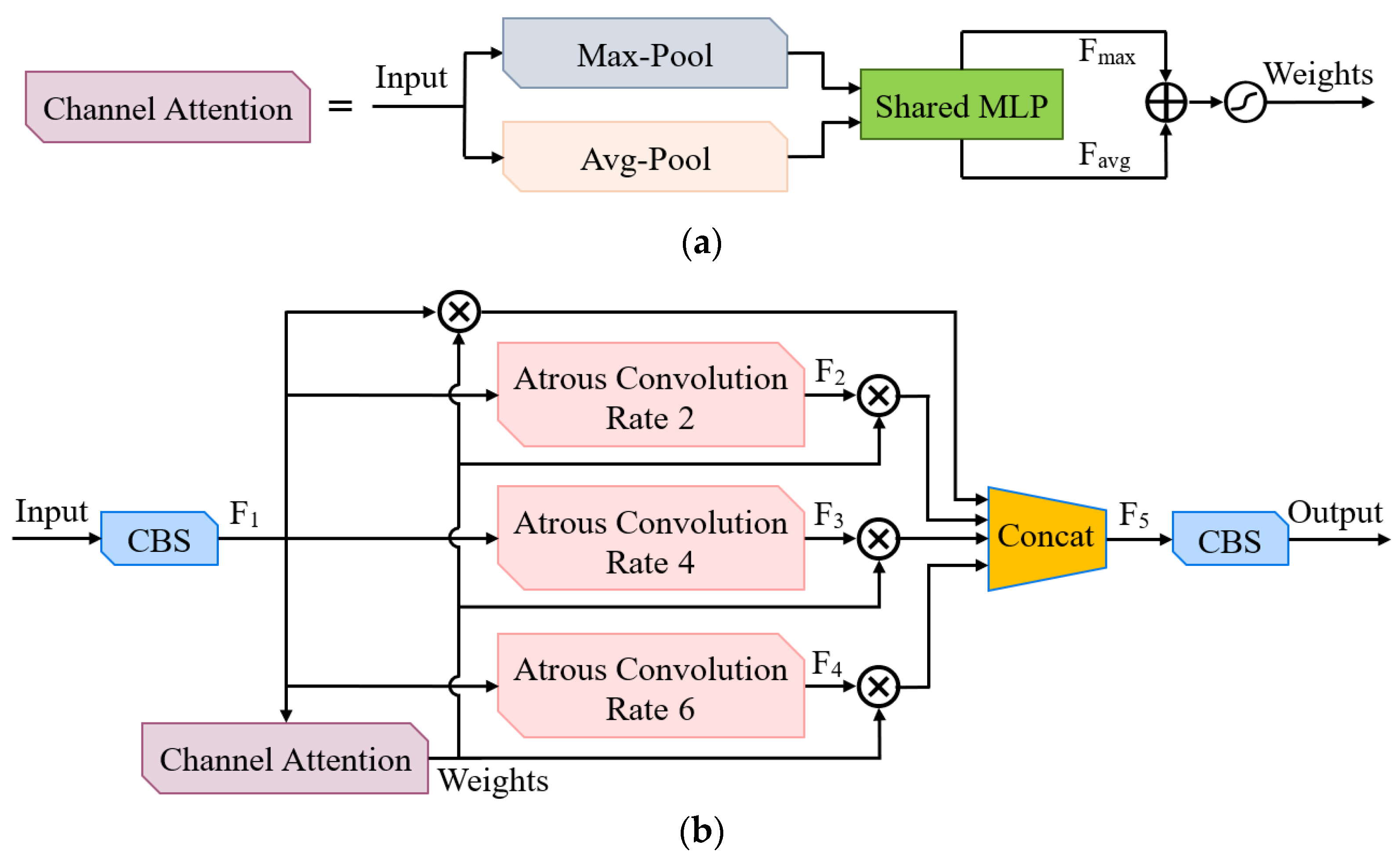
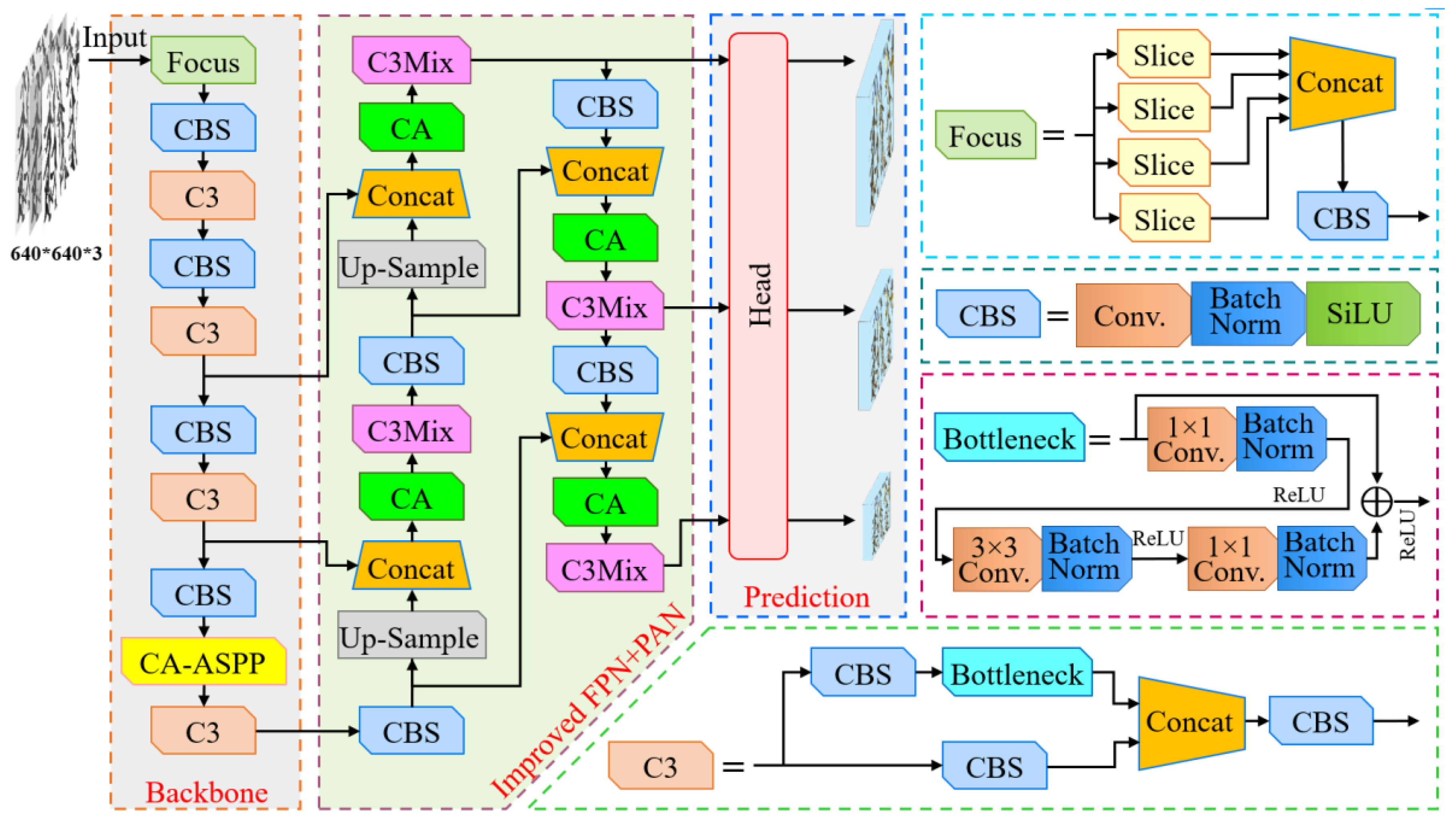
2.3.2. Improved YOLO-v5 Network Model

The original YOLO-v5 network has a high accuracy in the detection of large objects, such as pedestrians and vehicles. However, it does not perform well for objects that are relatively small or dense, such as the phenotyping of pods in soybean populations. This is because YOLO-v5 uses a path aggregation method to build the FPN+PAN neck network structure, integrate low-layer location information and high-layer semantic information, and uses the cross-stage partial bottleneck with a three convolutions (C3) module to extract features from the fused information.

However, when the FPN structure up samples from top to bottom, the path aggregation uses many features extracted earlier in the backbone network. Then, when extracting features, the FPN does not use a convolution kernel that can expand the receptive field and transfers features to the PAN network structure through path aggregation to predict targets. Due to the low network depth of the low-layer positioning information in the early stage of the network, there is an insufficient receptive field for small targets in complex environments, which leads to low detection accuracy of small targets and insufficient ability to distinguish between the background and foreground.

Therefore, based on YOLO-v5, an improved FPN+PAN structure is proposed by introducing a mixed depth convolution (MixConv) [37] to further improve the FPN+PAN structure. By further expanding the receptive field, the model can more accurately locate and identify phenotypic information of pods in soybean fields. We used a multilayer 3 × 3 convolution kernel instead of the large convolution kernel in MixConv to improve the receptive field and avoid a sharp increase in the model (as shown in Figure 8a,b). Then, the improved MixConv operation was used to replace the convolution operation in the convolution, batch normalization, and sigmoid-weighted linear unit (CBS) modules to construct mixed depth convolution, batch normalization, and sigmoid-weighted linear unit (MCBS) modules. Finally, the MCBS module was introduced into the C3 module to construct a C3Mix module. The module structure of the C3Mix module is shown in Figure 8c. First, the feature map F₁ was input into two CBS modules with a kernel size of 1 × 1 to obtain feature maps F₂ and F₃ by compressing the number of channels to prevent the number of channels from being too high after the concatenation operation, causing the size of the model to become larger. A CBS module with a kernel size of 1 × 1 was used for feature map F₂ to learn the cross-channel correlation and spatial correlation to realize a linear combination between channels and to enhance nonlinear characteristics. Then, the MCBS module was used to extract features under different receptive fields to obtain the feature map F₄ by looping N times. Finally, after concatenating feature maps F₃ and F₄, the output feature map F₅ of this module was obtained using a CBS module with a kernel size of 1 × 1 to change the number of channels of the concatenated feature. Through the C3Mix module, we enhanced the receptive field of the model and obtained the detailed positioning information of targets under different receptive fields, thereby improving the model’s positioning ability and the ability to distinguish between the background and foreground.

In dynamic detection for phenotyping pods, the model should detect all pods as often as possible. Therefore, the recall index of the model is very important. The original YOLO-v5 has difficulty meeting the requirements for recall in this case, partly because the repeated use of max pooling in the spatial pyramid pooling (SPP) module loses many target details, resulting in individual targets being considered background and cannot be detected. Based on atrous spatial pyramid pooling (ASPP) [38], we propose channel attention atrous spatial pyramid pooling (CA-ASPP), in which a channel attention (CA) mechanism is introduced to improve the model’s ability to extract multiscale detail features. The CA structure is shown in Figure 9a. The CA-ASPP network structure is shown in Figure 9b.

The channel number of the feature map inputted in CA-ASPP is squeezed by a CBS model with a kernel size of 1 × 1 to generate feature map F₁. Considering the loss of target details in the max pooling operation, we applied atrous convolution instead of pooling. The kernel size can be changed by adjusting the atrous rate. Feature maps F₂, F₃, and F₄ were obtained by applying a 3 × 3 filter to feature map F₁ with different atrous rates. In fact, they were the results of resampling to feature map F₁ at different scales, and they were similar in different channels. Thus, we applied a channel attention module [39] to exploit the interchannel relationship of features. Average pooling and max pooling are used in the channel attention module to squeeze the spatial dimension of the input feature map F₁ to aggregate the spatial information. The spatial information was then forwarded to a shared multilayer perceptron (MLP). After the output feature vectors were merged using elementwise summation, the sigmoid function was used to generate the weights of each channel. We took the weights to constrain each channel of feature maps F₁, F₂, F₃, and F₄ using elementwise multiplication and concatenated them to generate feature map F₅. Finally, to avoid a large channel number after concatenation, we squeezed the channel number of feature map F₅ using a CBS model with a kernel size of 1 × 1 again to generate the output feature. The CA-ASPP module obtained abundant multiscale semantic information through atrous convolution and focused on the importance of different features through channel attention to further enhance the semantic information.

To enable the positioning accuracy and identifiability of the model for soybean pods, a coordinate attention (CA) mechanism was introduced into the improved network model. First, a global pooling operation was performed in the width and height directions of the input feature map. Feature maps with a global receptive field were obtained, and the precise position information was encoded. The double direction feature maps were concatenated to generate coordinate attention in which the operation included convolution, batch normalization, and an activation function. We used a convolution operation with a 1 × 1 convolution kernel for the concatenated feature map according to the original width and height of the feature map to obtain two feature maps with the same number of channels as the original. After the sigmoid activation function, the attention weights of the feature map in height and width were obtained. Finally, the original feature map was weighted by multiplication, and the final feature map with attention weight in the width and height directions was obtained. Through the CA mechanism, the channel attention was decomposed into a one-dimensional feature encoding process in the horizontal and vertical directions. Direction sensing information and spatial location information were embedded into the generated feature map. Using this method, it was possible to capture not only channel information but also direction sensing information and location sensitive information so the model could more accurately locate and identify objects in the region of interest (ROI). The architecture of the improved YOLO-v5 for soybean pod detection is shown in Figure 10.

The binary cross-entropy (BCE) loss was applied in the calculation of confidence loss and classification loss in the original YOLO-v5. However, due to the significant imbalance between positive and negative samples of the target detector in the single-stage algorithm, the number of negative samples was much higher than that of positive samples, which leads to the loss calculation being dominated by negative samples and ultimately leading to a poor model training effect. The loss tends to learn from a large number of similar simple samples, which makes the training effect of difficult classification samples with complex sample distribution poor. Finally, the training time of the target detection model was usually longer. A loss function with faster convergence speed would help improve the training speed and obtain a better model faster. Therefore, the calculation of the confidence loss and classification loss in the improved YOLO-v5 model presented in this paper was executed using polynomial loss (PolyLoss) [40] based on focal loss. PolyLoss is a unified polynomial framework for the focal loss and BCE loss. The PolyLoss framework is shown in Equation (7). For the negative samples dominating the loss calculation caused by the high number of negative samples, we used $\alpha$ to balance the weights of the positive and negative samples. For the poor training effect of the BCE loss on hard-to-classify samples, we used $\gamma$ to increase the loss of samples classified difficultly to make the loss function pay more attention to samples classified difficultly. To improve the convergence speed of the model, the term ${\alpha }_t\epsilon {\left(1-P_t\right)}^{1+\gamma }$ was added to further increase the loss and greatly accelerate the convergence speed.

$$L_{Poly-L}=-{\alpha }_t{\left(1-P_t\right)}^{\gamma }\log \left(P_t\right)+{\alpha }_t\epsilon {\left(1-P_t\right)}^{1+\gamma },$$

(7)

where the value of ${\alpha }_t$ is $\alpha$ and the value of $P_t$ is $P\left(x\right)$, which represents the prediction result of the model for a positive sample, the value of ${\alpha }_t$ is $1-\alpha$ and the value of $P_t$ is $1-P_t$ for a negative sample.

With the PolyLoss, the model convergence could be accelerated. At the same time, more samples classified difficultly could be detected, and the recall rate could be improved due to the enhanced learning of difficult classification samples.

3. Results

3.1. Test Environment and Parameters

The soybean image VOC dataset was divided at 80%, 10%, and 10%, into training, validation, and test datasets, respectively. The training and validation datasets were input into the network for training. Adaptive momentum estimation (Adam) was applied to optimize the training model. The main model training parameters were set as follows: learning batch size = 32, momentum = 0.9, weight decay = 0.0005, and learning rate = 0.001. The main hardware parameters for the experiments were an Intel Core i7 9700 CPU (Intel Corp., Santa Clara, CA, USA), 16 GB random-access memory (RAM), Nvidia GeForce RTX A3000 GPU (Nvidia Corp., Santa Clara, CA, USA), and 6 GB video memory capacity. The compute unified device architecture (CUDA) version was 11.2. The operating system was Ubuntu 18.04 LTE (Canonical Ltd., London, UK). The integrated development environment (IDE) was Visual Studio Code. The programming language was Python 3.8, and the deep learning framework was PyTorch 1.8 (Linux Foundation, San Francisco, CA, USA). The detailed environment parameter configuration is shown in

Table 1. Test environment configuration.

No.	Parameter	Configuration
1	CPU	Intel Core i7 9700K
2	GPU	Nvidia GeForce RTX A3000, 6 GB VRAM
3	RAM	16 GB DDR4 3200 MHz
4	GPU accelerated environment	CUDA 11.2
5	Operating system	Ubuntu 18.04 LTE
6	IDE	Visual Studio Code 1.72.2
7	Deep learning framework	PyTorch 1.8
8	Benchmark model	YOLO-v5s
9	Computer vision library	OpenCV 4.5

.

3.2. Evaluation of Model Performance

To test the effectiveness of the improved model for soybean pod detection, we used the intersection over union (IOU) to evaluate the accuracy of the model according to the coincidence rate of the output box and the label box [41]. Because soybean pod targets are small, the IOU threshold value was set to 0.5 to reduce the loss of partial targets in detection. The precision, recall rate, mean average precision (mAP) @0.5 and mAP@0.5:0.95 were introduced in this study as evaluation indexes.

To comprehensively evaluate the model and to provide a basis for the selection of the optimal model, a weighted evaluation model OPT was established as follows.

$$IOU=\frac{area\left(B_P{\displaystyle \cap }{B}_{gt}\right)}{area\left(B_P{\displaystyle \cup }{B}_{gt}\right)},$$

(8)

$$PR=\frac{TP}{TP+FP}\times 100\%,$$

(9)

$$RE=\frac{TP}{TP+FN}\times 100\%,$$

(10)

$$AP={{\displaystyle \int }}_0^{1}PR\left(r\right)dr,$$

(11)

$$mAP=\frac{1}{N_{class}}{{\displaystyle \sum }}_{i=1}^{N_{class}}A{P}_i,$$

(12)

$$OPT=w_1·PR+w_2·RE+w_3·mAP@0.5+w_4·mAP@0.5:0.95,$$

(13)

where $B_P$ and $B_{gt}$ are the predicted anchor and actual anchor of a target, respectively, and IOU is the degree of overlap between the two anchors. PR and RE represent the precision and recall rate, respectively. TP, FP, and FN represent the number of correctly detected, incorrectly detected, and missing frames, respectively. The AP value represents the area under the precision–recall (P–R) curve. The mAP value was obtained by averaging all AP categories, and $N_{class}$ represents the total number of types detected. $w_i \left(i=1,2,3,4\right)$ refers to the weight of each parameter.

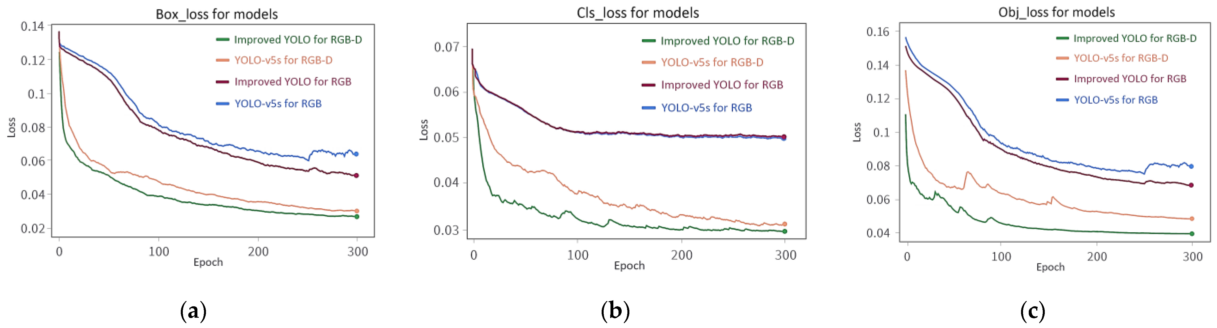
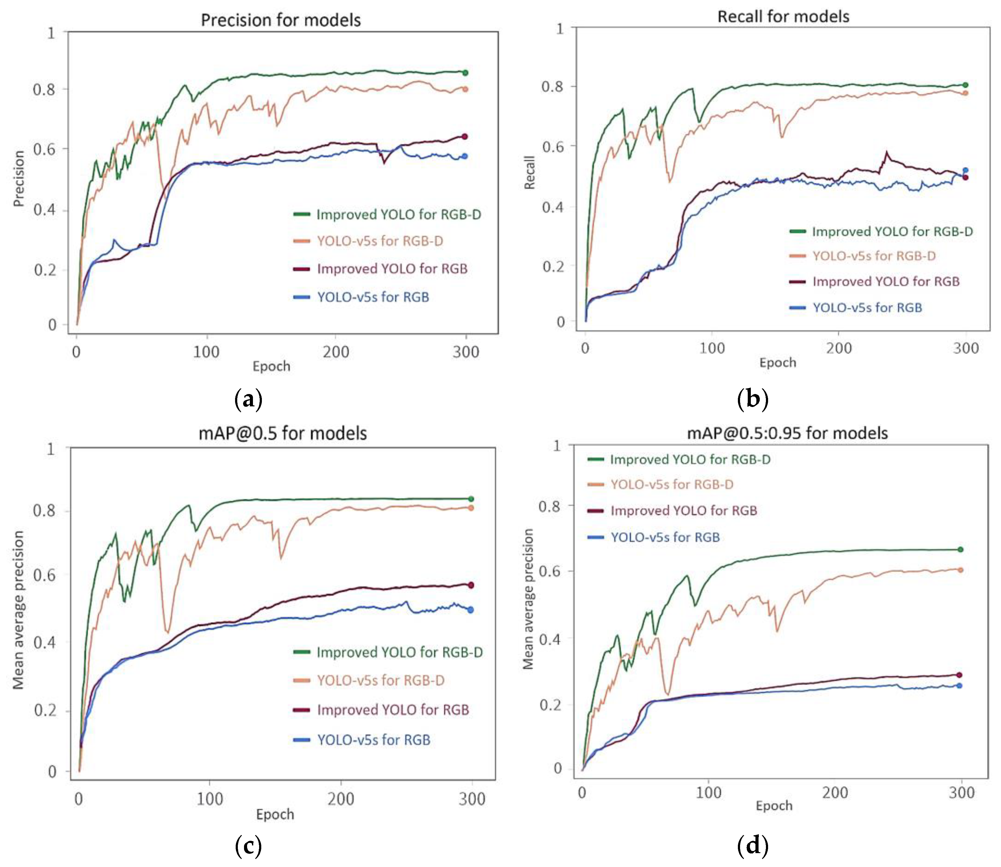
3.3. Analysis of Model Training for Different Datasets

To analyze the effectiveness of using soybean RGB-depth fusion images to distinguish the background to improve the soybean pod detection model in a complex field environment, we used the RGB image and RGB-D fusion image datasets to train YOLO-v5s and the improved YOLO-v5 network. The subset ratio, labels, target positions, and classification of both image datasets were completely consistent. Compared with the training RGB image dataset, the difference was that the soybean image background in the RGB-D dataset was eliminated based on depth image data before the dataset was input into the network model, where the depth image data are three-dimensional point cloud data that only contain the distance and position information from the targets to the sensor without RGB data.

Figure 11 shows that as the number of iterations increased, the training loss value of the model gradually decreased. The box loss indicates whether the detection target is covered by the predicted bounding box. The object loss is a measure of the probability that the detection target exists in the region of interest. The classification loss represents the ability to correctly predict a given object category. The smaller the loss values of these three indexes are, the more accurate the prediction of the model in each index. After 50 iterations, the loss values of the improved YOLO-v5 and YOLO-v5s on the RGB-D dataset, and the improved YOLO-v5 and YOLO-v5s on the RGB dataset decreased slowly. When the number of iterations reached approximately 200, the loss curve was almost flat. Compared with the improved YOLO-v5 and YOLO-v5s on the RGB-D dataset, the loss values of the improved YOLO-v5 and YOLO-v5s on the RGB dataset were significantly higher, so the predictions of these two models were relatively low, which can also be clearly seen in Figure 12. Therefore, in the complex background environment of soybean fields, network models based on only training RGB image datasets could not meet the soybean pod recognition requirements. This is because the complex background of stems, branches, leaves, etc., in a field will seriously affect the feature recognition of soybean pods, which is the main factor affecting the recognition accuracy of soybean pods in the field. In contrast, processing the background in RGB-D images through depth data can significantly improve soybean pod feature recognition within the recognition range.

Under the same testing parameters, the RGB-D dataset was used to train the improved YOLO-v5 and YOLO-v5s networks. From Figure 12, compared with the improved YOLO-v5 and YOLO-v5s based on the RGB dataset, the improved YOLO-v5 and YOLO-v5s based on the RGB-D dataset had significant improvement in the recall rate and precision for soybean pod target detection, where the recall increased by approximately 32% and the precision increased by approximately 25%. The precision of the improved YOLO-v5 based on the RGB-D dataset was approximately 6% higher than that of YOLO-v5s based on the RGB-D dataset. This is because our improved FPN+PAN structure and CA-ASPP module in the network improved the small target detection ability and distinguished between the background and foreground.

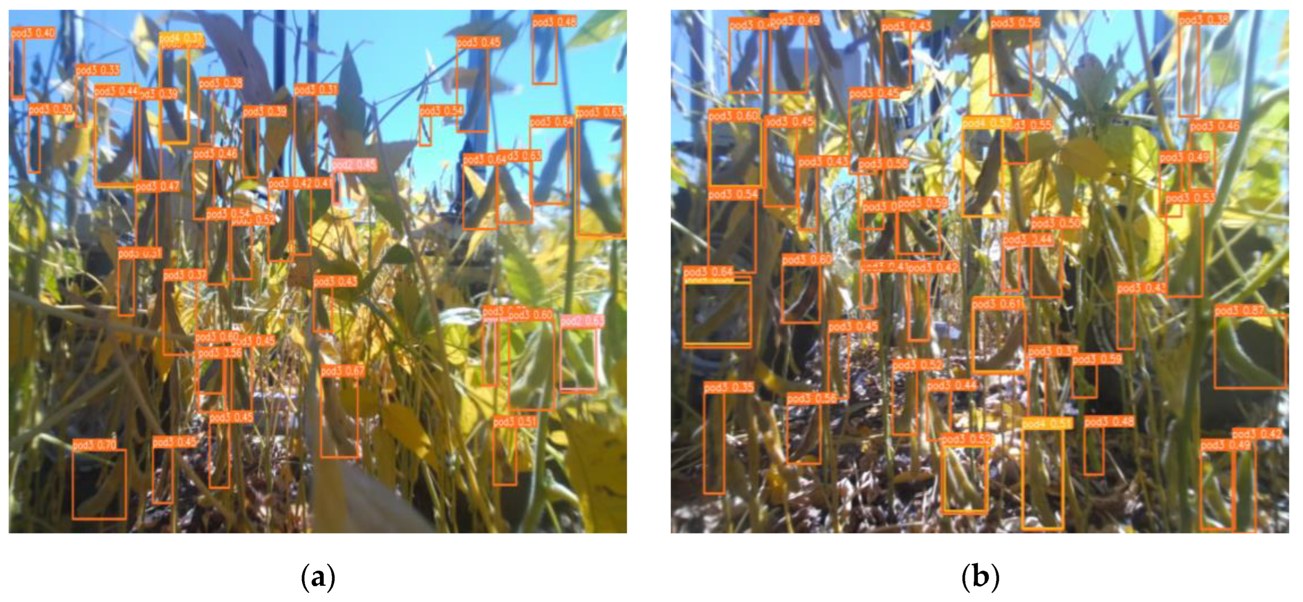
3.4. Analysis of Dynamic Detection Phenotyping of Pods in the Field

We applied the improved YOLO-v5 model to the soybean pod phenotyping detection system on the field soybean image acquisition vehicle to carry out field experiments for testing and analyzing the model performance by comparing model prediction values and manual measurement values. Some biological characteristics of the experimental objects, experimental locations, and conditions were discussed in Section 2.1 of this paper.

Considering the influence of the soybean population on the test data, the experimental soybean populations of Longken 3401 and Heihe 43 in the experimental area were separately divided into 10 groups. The number of individual plants in each group ranged from 20 to 200. In testing, the classification and quantity of soybean pods were detected by manual measurement and identification model prediction.

The identification model detection process was dynamic as the vehicle moved and the Kinect DK sensor on a servo linear rail moved up and down. To ensure that the soybean pods are detected as accurately as possible, the target position was dynamically tracked to avoid repeated counting of the same target during detection. The partial pod dynamic detection is shown in Figure 13.

Table 2. Soybean pod number test results for each test group.

No. of Test Group	Total Number of Soybean Plants in Each Test Group	Average Number of Soybean Pods per Plant of Different Varieties
		Longken 3401	Heihe 43	Longken 3401	Heihe 43
		Identification Model Prediction Values (pcs/per Plant)		Manual Measurement Values (pcs/per Plant)
1	20	12.23	13.31	23.62	27.62
2	40	10.21	18.36	21.81	29.10
3	60	8.19	16.22	21.03	28.27
4	80	11.00	14.87	22.54	27.79
5	100	13.27	17.13	20.18	30.41
6	120	14.05	21.21	23.57	29.30
7	140	18.29	23.83	23.71	29.01
8	160	19.83	22.62	25.43	30.22
9	180	21.71	24.50	27.87	30.18
10	200	20.52	25.38	26.65	30.44

shows that the prediction values from the identification model are obviously lower than the manual measurement values. The main influence in detecting soybean pods is that dense plants often overlap and cover pods. However, after statistical data analysis, when the total number of soybean populations tested is small at the R6 stage, the rate of missed detection of soybean pods fluctuates between 30–50%. With the increase in the number of individuals in the soybean population for detection, the deviation is basically stable at approximately 20% (as shown in Figure 14a). By establishing the correlation between the predicted value and the manually measured value, the coefficient of determination between the predicted average value of the number of soybean pods per plant of the two varieties and the manually measured average value was 0.9752 with a certain bias when the total number of soybean plants in the tested soybean population was more than 140 (as shown in the shaded area in Figure 14b).

Therefore, we tried to establish a soybean pod quantity compensation model as follows for a dynamic detection system to statistically correct the pod prediction quantity. To verify the effectiveness of the soybean pod quantity compensation method, Equations (14)–(17) were used to calculate the relative error and mean relative error between the predicted and manually measured pod quantity values.

$${\overline{P}}_{pod}=\frac{P_{pod}}{M_{plant}}+K,$$

(14)

$$K=\frac{M_{pod}-P_{pod}}{M_{plant}}\times P_{pod},$$

(15)

$$P_i=\frac{\left|x_i-{\overline{x}}_i\right|}{{\overline{x}}_i}\times 100\%,$$

(16)

$$R=\frac{1}{m}{{\displaystyle \sum }}_{i=1}^m{p}_i\times 100\%,$$

(17)

where ${\overline{P}}_{pod}$ represents the average number of pods per plant predicted by the identification model, $P_{pod}$ represents the total number of pods predicted by the model, $M_{plant}$ represents the total number of individual plants in the soybean population within the detection range, $K$ is the pod quantity compensation factor, and $M_{pod}$ is the actual total number of pods manually measured. $P_i$ represents the relative error in the calculation of the average number of pods per plant, $R$ represents the mean relative error in the calculation of the average number of pods per plant, $x_i$ represents the predicted value of the average number of pods per plant, ${\overline{x}}_i$ represents the manually measured value of the average number of pods per plant, and $m$ represents the number of plants of each test variety group.

Thus, we can correct the number of pods predicted using the soybean pod quantity compensation model. Each classification pod quantity can be rectified according to the proportion of pods of each category to the total number of pods. Figure 15 shows that after pod quantity compensation, the coefficient between the predicted average value and the manually measured average value of different classification pod numbers was 0.9866. From the predicted number distribution of different classification pods per plant in partially tested soybean plants of Heihe 43 and Longken 3401 (as shown in Figure 16), the number of pods with three seeds was largest, followed by pods with two seeds, four seeds, and one seed. The category with the fewest pods was empty pods. The average number of pods per plant of Heihe 43 was 22.64% higher than that of Longken 3401. The trend of the predicted value of the number of pods was basically consistent with that of the manually measured value. According to Equation (17), the mean relative errors between the predicted and manually measured numbers of pods were 2.12% for Heihe 43 and 2.74% for Longken 3401.

4. Discussion

This paper presented a method for dynamic pod phenotyping detection in soybean populations based on an improved YOLO-v5 network, including pod classification, quantity, and number distribution of different classification pods in soybean populations. To reduce the impact on model detection accuracy from the complex background of the natural environment, we established an RGB-D dataset by using the fusion of RGB and depth image data to train the network model. Although the detection accuracy of the model in a leaf-covering and pod-overlapping situation will be affected, the soybean pod quantity compensation algorithm proposed in this paper can statistically correct the number of pods to improve the prediction accuracy to a certain extent.

To verify the effectiveness of the proposed method, YOLO-V5s, Faster-RCNN, SSD and our improved model were used to detect pods in the soybean population from the R6 to R7 stages without applying the compensation method under the same test environment and same training dataset. The detection results are shown in

Table 3. Comparison of model detection results.

Number of Plants in Soybean Population	Experimental Model	Evaluation Indicators (Unit: %)
		Precision	Recall	mAP@0.5	mAP@0.5:0.95
20	Improved YOLO-v5	82.72	74.54	81.26	52.43
	YOLO-v5s [35]	77.13	73.92	76.47	50.17
	Faster-RCNN [20]	76.65	71.39	73.15	47.24
	SSD [23]	71.49	67.08	68.26	45.58
80	Improved YOLO-v5	83.50	74.63	80.95	51.75
	YOLO-V5s [35]	81.14	71.57	77.02	47.32
	Faster-RCNN [20]	74.82	70.34	71.33	46.50
	SSD [23]	71.95	68.87	69.43	44.21
140	Improved YOLO-v5	86.26	77.66	85.31	53.20
	YOLO-V5s [35]	81.91	74.33	81.12	51.19
	Faster-RCNN [20]	76.76	72.00	73.12	45.99
	SSD [23]	71.09	67.51	70.08	42.16
200	Improved YOLO-v5	88.14	78.35	87.87	58.53
	YOLO-V5s [35]	82.10	74.97	82.90	54.67
	Faster-RCNN [20]	75.98	71.26	74.55	48.35
	SSD [23]	72.11	69.73	70.70	43.40

. In this soybean growing stage, soybean leaves are still relatively dense, which is the main factor affecting the detection of pods in the field. Therefore, the prediction accuracies of all four models were generally low.

When the number of plants in the soybean population tested was relatively large, the prediction accuracies of the models were slightly improved due to the exclusion of the influence of individual plant differences, and the precision improvement of our model was relatively obvious, reaching a precision of 88.14% and a recall rate of 78.35%. This was because our model is more sensitive to the perception of small soybean pod targets. The results showed that our proposed method improved the model’s detection ability. The effectiveness of this method was verified, and good experimental results were obtained.

5. Conclusions

The accurate of phenotyping description of pods in soybean populations in a natural environment is of great significance to soybean breeding and soybean yield and quality estimation. In this paper, a dynamic detection method for phenotyping pods in soybean populations in the field based on an improved YOLO-v5 network was proposed, including the pod classification, quantity, and number distribution of different classification pods in soybean populations. According to the experimental results, the conclusions can be summarized as follows:

(1)

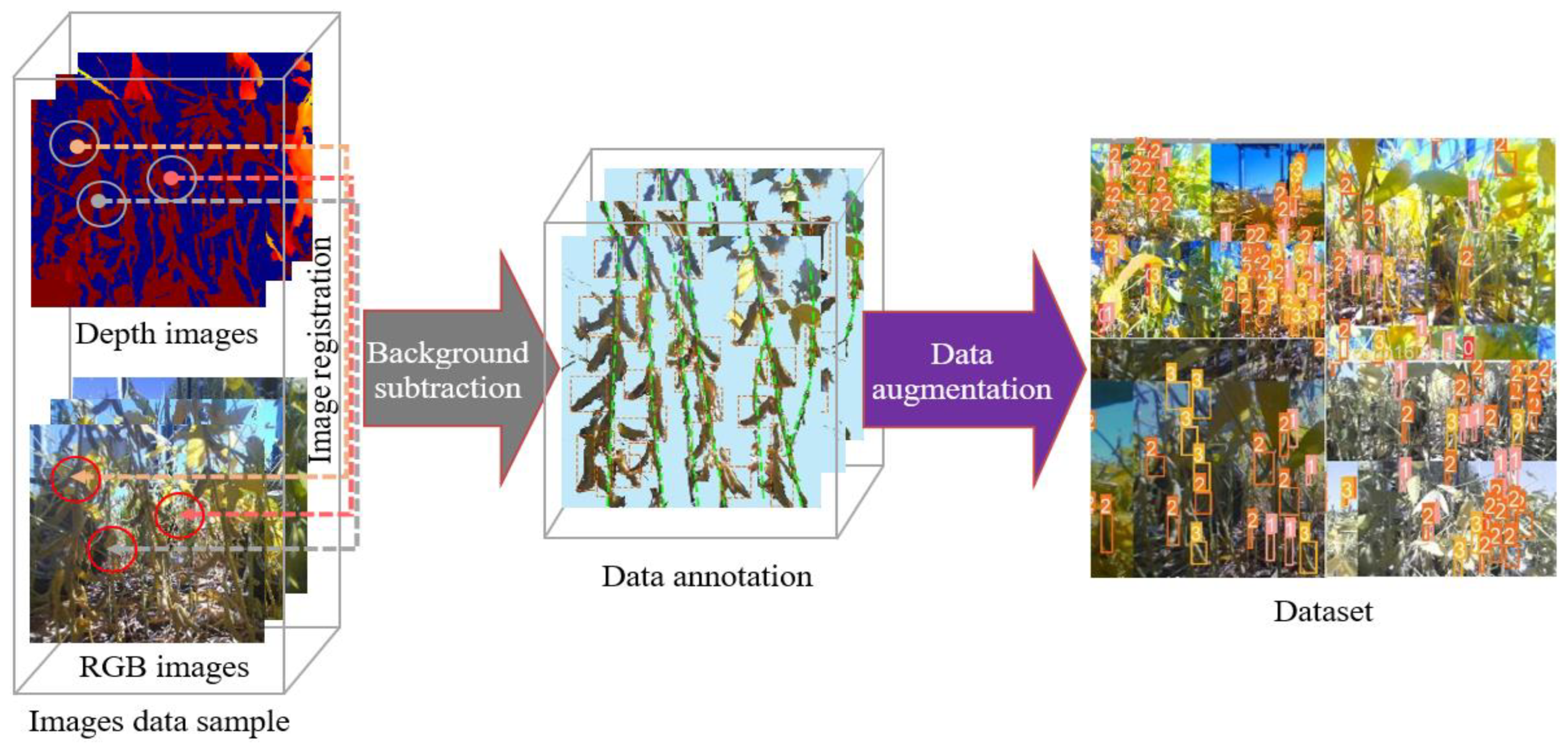
The complex background of the natural environment greatly affected the detection of phenotypic traits of soybean pods. An RGB-depth fusion method to distinguish background could effectively improve the model performance for detecting soybean pods in complex field environments. Compared with network models trained on the RGB dataset, the recall and precision of models trained on the RGB-D dataset were increased by approximately 32% and 25%, respectively.

(2)

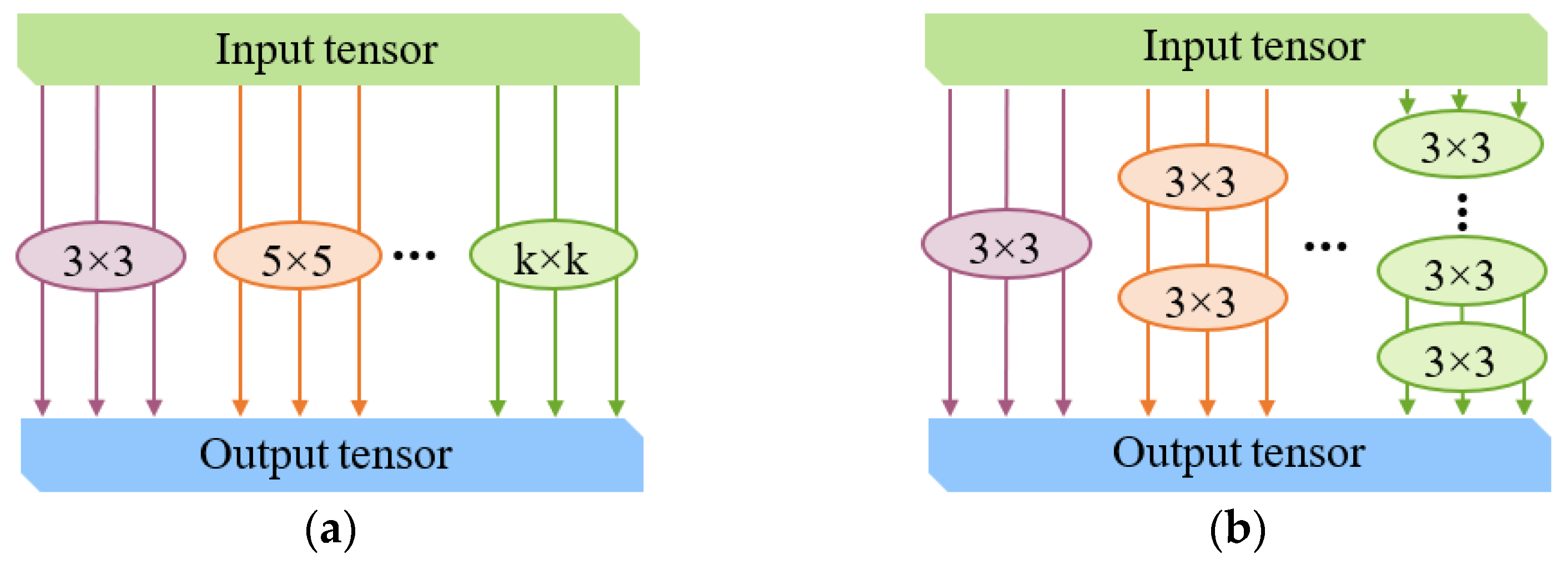
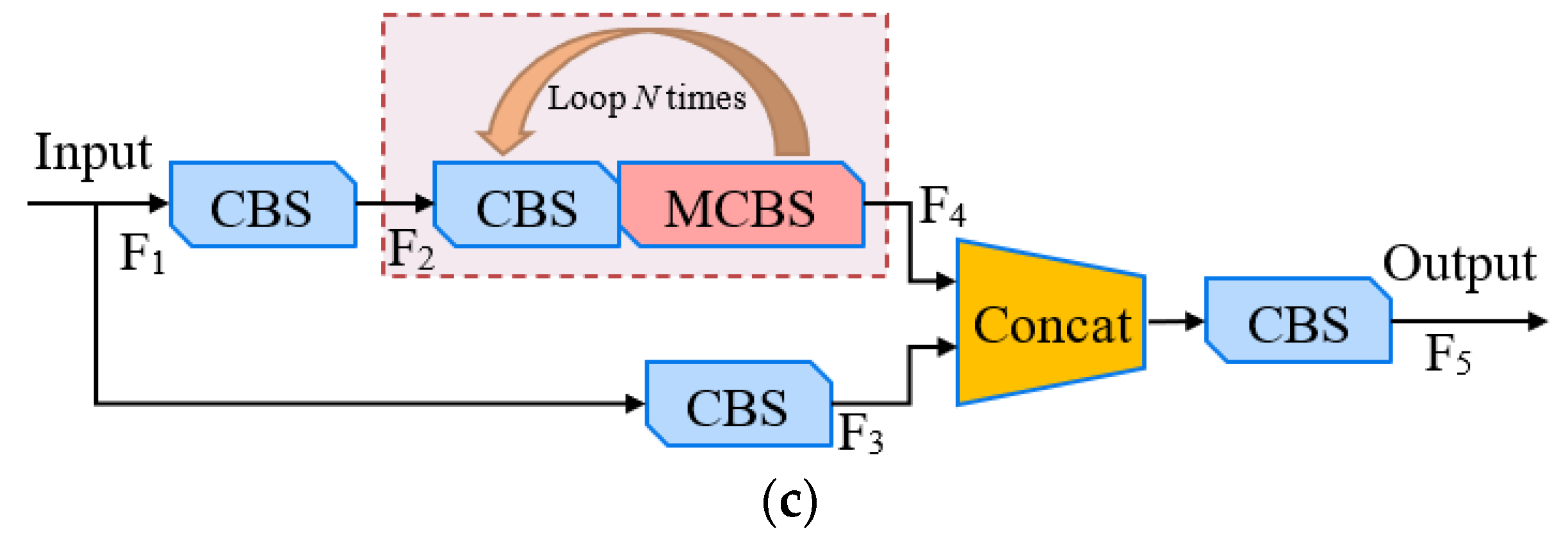
The improved YOLO-v5 network model established by introducing the improved FPN+PAN structure and CA-ASPP module had the further ability to detect small targets and distinguish between the background and foreground. Compared with YOLO-v5s, the precision of the improved YOLO-v5 increased by approximately 6%, reaching 88.14% precision for pod number detection for the 200 plants in the soybean population tested.

(3)

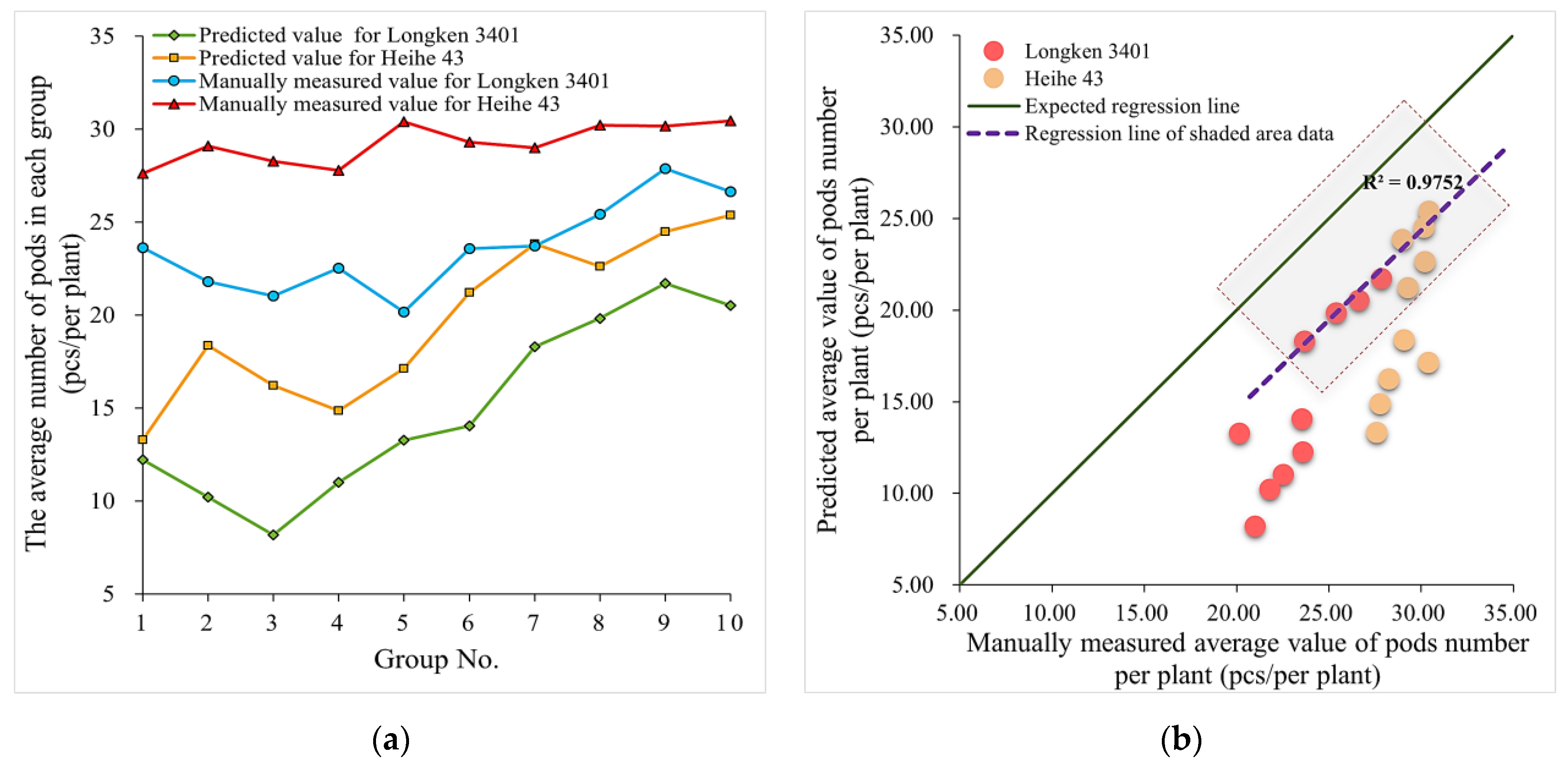
A soybean pod quantity compensation model was established by analyzing the influence of the number of individual plants in the soybean population on the detection precision of models to statistically correct various pod prediction quantities. The testing showed that after compensation calculation, the mean relative errors between the predicted and actual pod numbers were 2% to 3% for the two tested soybean varieties.

The method proposed in this paper solves the problems of low efficiency, precision, and sample size of soybean phenotypes collected by manual sampling in the field, which provides technical support for the scientific regulation and big data analysis of ecological and morphological traits in soybean variety breeding, cultivation, and management. Although our improved YOLO-v5 network achieved good results for phenotyping detection of soybean pods in soybean populations, the ecological differences of soybean varieties in different growth periods still have a certain impact on the phenotyping detection of pods. In addition, to some extent, the compensation method proposed is affected by different models and varieties. In future research, we will continue to expand our research to include more soybean varieties, improve compensation methods, and optimize the network performance to increase the scope of application.

References

1. Yang, S.; Zheng, L.; Yang, H.; Zhang, M.; Wu, T.; Sun, S.; Tomasetto, F.; Wang, M. A Synthetic Datasets Based Instance Segmentation Network for High-Throughput Soybean Pods Phenotype Investigation. Expert Syst. Appl. 2022, 192, 116403. [Google Scholar] [CrossRef]
2. Lu, W.; Du, R.; Niu, P.; Xing, G.; Luo, H.; Deng, Y.; Shu, L. Soybean Yield Preharvest Prediction Based on Bean Pods and Leaves Image Recognition Using Deep Learning Neural Network Combined With GRNN. Front. Plant Sci. 2022, 12, 791256. [Google Scholar] [CrossRef] [PubMed]
3. Momin, M.A.; Yamamoto, K.; Miyamoto, M.; Kondo, N.; Grift, T. Machine Vision Based Soybean Quality Evaluation. Comput. Electron. Agric. 2017, 140, 452–460. [Google Scholar] [CrossRef]
4. Jiang, S.; An, H.; Luo, J.; Wang, X.; Shi, C.; Xu, F. Comparative Analysis of Transcriptomes to Identify Genes Associated with Fruit Size in the Early Stage of Fruit Development in Pyrus Pyrifolia. Int. J. Mol. Sci. 2018, 19, 2342. [Google Scholar] [CrossRef] [PubMed] [Green Version]
5. Rahman, S.U.; McCoy, E.; Raza, G.; Ali, Z.; Mansoor, S.; Amin, I. Improvement of Soybean; A Way Forward Transition from Genetic Engineering to New Plant Breeding Technologies. Mol. Biotechnol. 2022, 64, 1–19. [Google Scholar] [CrossRef]
6. Wang, Y.-H.; Su, W.-H. Convolutional Neural Networks in Computer Vision for Grain Crop Phenotyping: A Review. Agronomy 2022, 12, 2659. [Google Scholar] [CrossRef]
7. Zhou, S.; Mou, H.; Zhou, J.; Zhou, J.; Ye, H.; Nguyen, H.T. Development of an Automated Plant Phenotyping System for Evaluation of Salt Tolerance in Soybean. Comput. Electron. Agric. 2021, 182, 106001. [Google Scholar] [CrossRef]
8. Yassue, R.M.; Galli, G.; Borsato, R., Jr.; Cheng, H.; Morota, G.; Fritsche-Neto, R. A Low-Cost Greenhouse-Based High-Throughput Phenotyping Platform for Genetic Studies: A Case Study in Maize under Inoculation with Plant Growth-Promoting Bacteria. Plant Phenome J. 2022, 5, e20043. [Google Scholar] [CrossRef]
9. Warman, C.; Sullivan, C.M.; Preece, J.; Buchanan, M.E.; Vejlupkova, Z.; Jaiswal, P.; Fowler, J.E. A Cost-Effective Maize Ear Phenotyping Platform Enables Rapid Categorization and Quantification of Kernels. Plant J. 2021, 106, 566–579. [Google Scholar] [CrossRef]
10. Ban, S.; Liu, W.; Tian, M.; Wang, Q.; Yuan, T.; Chang, Q.; Li, L. Rice Leaf Chlorophyll Content Estimation Using UAV-Based Spectral Images in Different Regions. Agronomy 2022, 12, 2832. [Google Scholar] [CrossRef]
11. Deery, D.; Jimenez-Berni, J.; Jones, H.; Sirault, X.; Furbank, R. Proximal Remote Sensing Buggies and Potential Applications for Field-Based Phenotyping. Agronomy 2014, 4, 349–379. [Google Scholar] [CrossRef] [Green Version]
12. Hu, F.; Lin, C.; Peng, J.; Wang, J.; Zhai, R. Rapeseed Leaf Estimation Methods at Field Scale by Using Terrestrial LiDAR Point Cloud. Agronomy 2022, 12, 2409. [Google Scholar] [CrossRef]
13. Thompson, A.L.; Thorp, K.R.; Conley, M.M.; Elshikha, D.M.; French, A.N.; Andrade-Sanchez, P.; Pauli, D. Comparing Nadir and Multi-Angle View Sensor Technologies for Measuring in-Field Plant Height of Upland Cotton. Remote Sens. 2019, 11, 700. [Google Scholar] [CrossRef] [Green Version]
14. Shafiekhani, A.; Kadam, S.; Fritschi, F.B.; DeSouza, G.N. Vinobot and Vinoculer: Two Robotic Platforms for High-Throughput Field Phenotyping. Sensors 2017, 17, 214. [Google Scholar] [CrossRef] [PubMed]
15. Herzig, P.; Borrmann, P.; Knauer, U.; Klück, H.-C.; Kilias, D.; Seiffert, U.; Pillen, K.; Maurer, A. Evaluation of RGB and Multispectral Unmanned Aerial Vehicle (UAV) Imagery for High-Throughput Phenotyping and Yield Prediction in Barley Breeding. Remote Sens. 2021, 13, 2670. [Google Scholar] [CrossRef]
16. He, H.; Ma, X.; Guan, H. A Calculation Method of Phenotypic Traits of Soybean Pods Based on Image Processing Technology. Ecol. Inform. 2022, 69, 101676. [Google Scholar] [CrossRef]
17. Chen, J.; Wang, Z.; Wu, J.; Hu, Q.; Zhao, C.; Tan, C.; Teng, L.; Luo, T. An Improved Yolov3 Based on Dual Path Network for Cherry Tomatoes Detection. J. Food Process Eng. 2021, 44, e13803. [Google Scholar] [CrossRef]
18. Zhang, Y.; Yu, J.; Chen, Y.; Yang, W.; Zhang, W.; He, Y. Real-Time Strawberry Detection Using Deep Neural Networks on Embedded System (Rtsd-Net): An Edge AI Application. Comput. Electron. Agric. 2022, 192, 106586. [Google Scholar] [CrossRef]
19. Girshick, R.; Donahue, J.; Darrell, T.; Malik, J. Rich Feature Hierarchies for Accurate Object Detection and Semantic Segmentation. In Proceedings of the IEEE Conference on Computer Vision and Pattern Recognition, Columbus, OH, USA, 23–28 June 2014; pp. 580–587. [Google Scholar]
20. Ren, S.; He, K.; Girshick, R.; Sun, J. Faster R-Cnn: Towards Real-Time Object Detection with Region Proposal Networks. Adv. Neural Inf. Process. Syst. 2015, 28, 1–9. [Google Scholar] [CrossRef] [Green Version]
21. He, K.; Gkioxari, G.; Dollár, P.; Girshick, R. Mask R-Cnn. In Proceedings of the IEEE International Conference on Computer Vision, Venice, Italy, 22–29 October 2017; pp. 2961–2969. [Google Scholar]
22. Fu, X.; Meng, Z.; Wang, Z.; Yin, X.; Wang, C. Dynamic potato identification and cleaning method based on RGB-D. Eng. Agríc. 2022, 42, e20220010. [Google Scholar] [CrossRef]
23. Liu, W.; Anguelov, D.; Erhan, D.; Szegedy, C.; Reed, S.; Fu, C.-Y.; Berg, A.C. Ssd: Single Shot Multibox Detector. In Proceedings of the European Conference on Computer Vision; Springer: Berlin/Heidelberg, Germany, 2016; pp. 21–37. [Google Scholar] [CrossRef] [Green Version]
24. Redmon, J.; Divvala, S.; Girshick, R.; Farhadi, A. You Only Look Once: Unified, Real-Time Object Detection. In Proceedings of the 2016 IEEE Conference on Computer Vision and Pattern Recognition (CVPR); IEEE: Las Vegas, NV, USA, 2016; pp. 779–788. [Google Scholar]
25. Redmon, J.; Farhadi, A. Yolov3: An Incremental Improvement. arXiv 2018, arXiv:1804.02767. [Google Scholar] [CrossRef]
26. Bochkovskiy, A.; Wang, C.-Y.; Liao, H.-Y.M. Yolov4: Optimal Speed and Accuracy of Object Detection. arXiv 2020, arXiv:2004.10934. [Google Scholar] [CrossRef]
27. Guo, X.; Qiu, Y.; Nettleton, D.; Yeh, C.-T.; Zheng, Z.; Hey, S.; Schnable, P.S. KAT4IA: K-Means Assisted Training for Image Analysis of Field-Grown Plant Phenotypes. Plant Phenomics 2021, 2021, 9805489. [Google Scholar] [CrossRef] [PubMed]
28. Guo, R.; Chongyu, Y.; Hong, H. Detection Method of Soybean Pod Number per Plant Using Improved YOLOv4 Algorithm. Trans. Chin. Soc. Agric. Eng. 2021, 37, 179–187. [Google Scholar]
29. Li, R.; Wu, Y. Improved YOLO v5 Wheat Ear Detection Algorithm Based on Attention Mechanism. Electronics 2022, 11, 1673. [Google Scholar] [CrossRef]
30. Ren, F.; Zhang, Y.; Liu, X.; Zhang, Y.; Liu, Y.; Zhang, F. Identification of Plant Stomata Based on YOLO v5 Deep Learning Model. In Proceedings of the 2021 5th International Conference on Computer Science and Artificial Intelligence, Beijing, China, 4–6 December 2021; pp. 78–83. [Google Scholar] [CrossRef]
31. Pathoumthong, P.; Zhang, Z.; Roy, S.; El Habti, A. Rapid Non-Destructive Method to Phenotype Stomatal Traits. bioRxiv 2022. [Google Scholar] [CrossRef]
32. Weerasekara, I.; Sinniah, U.R.; Namasivayam, P.; Nazli, M.H.; Abdurahman, S.A.; Ghazali, M.N. The Influence of Seed Production Environment on Seed Development and Quality of Soybean (Glycine max (L.) Merrill). Agronomy 2021, 11, 1430. [Google Scholar] [CrossRef]
33. Xia, S.; Li, M. A Novel Image Edge Detection Algorithm Based on Multi-Scale Hybrid Wavelet Transform. In Proceedings of the International Conference on Neural Networks, Information, and Communication Engineering (NNICE), Qingdao, China, 25–27 March 2022; SPIE: Washington, DC, USA, 2022; Volume 12258, pp. 505–510. [Google Scholar] [CrossRef]
34. Zhao, Y.; Shi, Y.; Wang, Z. The Improved YOLOV5 Algorithm and Its Application in Small Target Detection. In Proceedings of the Intelligent Robotics and Applications; Liu, H., Yin, Z., Liu, L., Jiang, L., Gu, G., Wu, X., Ren, W., Eds.; Springer International Publishing: Cham, Switzerland, 2022; pp. 679–688. [Google Scholar] [CrossRef]
35. Zhang, C.; Ding, H.; Shi, Q.; Wang, Y. Grape Cluster Real-Time Detection in Complex Natural Scenes Based on YOLOv5s Deep Learning Network. Agriculture 2022, 12, 1242. [Google Scholar] [CrossRef]
36. Wang, D.; He, D. Channel Pruned YOLO V5s-Based Deep Learning Approach for Rapid and Accurate Apple Fruitlet Detection before Fruit Thinning. Biosyst. Eng. 2021, 210, 271–281. [Google Scholar] [CrossRef]
37. Tan, M.; Le, Q.V. Mixconv: Mixed Depthwise Convolutional Kernels. arXiv 2019, arXiv:1907.09595. [Google Scholar] [CrossRef]
38. Chen, L.-C.; Papandreou, G.; Schroff, F.; Adam, H. Rethinking Atrous Convolution for Semantic Image Segmentation. arXiv 2017, arXiv:1706.05587. [Google Scholar] [CrossRef]
39. Woo, S.; Park, J.; Lee, J.-Y.; Kweon, I.S. Cbam: Convolutional Block Attention Module. In Proceedings of the European Conference on Computer Vision (ECCV), Munich, Germany, 8–14 September 2018; pp. 3–19. [Google Scholar]
40. Leng, Z.; Tan, M.; Liu, C.; Cubuk, E.D.; Shi, X.; Cheng, S.; Anguelov, D. PolyLoss: A Polynomial Expansion Perspective of Classification Loss Functions. arXiv 2022, arXiv:2204.12511. [Google Scholar] [CrossRef]
41. Zhang, Y.-F.; Ren, W.; Zhang, Z.; Jia, Z.; Wang, L.; Tan, T. Focal and Efficient IOU Loss for Accurate Bounding Box Regression. Neurocomputing 2022, 506, 146–157. [Google Scholar] [CrossRef]
Figure 1. Field soybean three-dimensional color image acquisition vehicle. (a) Drawing of the structure; (b) Photo of the structure in situ.
Agronomy 12 03209 g001
Figure 2. Samples of RGB and depth image data.
Agronomy 12 03209 g002
Figure 3. Extracting sub feature images.
Agronomy 12 03209 g003
Figure 4. RGB and depth image registration. (a) Depth image; (b) gray depth image; (c) RGB image; (d) gray image; (e) registered image; (f) angle histogram of feature point pairs; and (g) feature point pair alignment metric.
Agronomy 12 03209 g004
Figure 5. Classification diagram of different pod morphologies. (a) Empty pod; (b) pod with one seed; (c) pod with two seeds; (d) pod with three seeds; and (e) pod with four seeds.
Agronomy 12 03209 g005
Figure 6. Quantity distribution map for different pod morphologies.
Agronomy 12 03209 g006
Figure 7. Image data processing.
Agronomy 12 03209 g007
Figure 8. Module structure. (a) MixConv; (b) improved MixConv; and (c) C3Mix.
Agronomy 12 03209 g008aAgronomy 12 03209 g008b
Figure 9. Module network structure. (a) CA; and (b) CA-ASPP.
Agronomy 12 03209 g009
Figure 10. Architecture of the improved YOLO-v5 for soybean pod detection.
Agronomy 12 03209 g010
Figure 11. Training loss curves. (a) Box loss for models; (b) classification loss for models; and (c) object loss for models.
Agronomy 12 03209 g011
Figure 12. Training process curves. (a) Precision for models, (b) recall for models, (c) mean average precision at 0.5 for models, and (d) mean average precision at 0.5 to 0.95 for models.
Agronomy 12 03209 g012
Figure 13. Dynamic detection phenotyping of pods in the field. (a) The image sensor running to the upper part of the soybean population for detection; (b) The image sensor running to the lower part of the soybean population for detection.
Agronomy 12 03209 g013
Figure 14. Relation between identification model prediction values and manually measured values of two varieties. (a) The change curve of the average number of pods in the test groups; (b) Linear correlation between the identification model pod number prediction and the manually measured values of the two varieties.
Agronomy 12 03209 g014
Figure 15. Linear correlation between the predicted average value and manually measured average value of the number of different classification pods after pod quantity compensation.
Agronomy 12 03209 g015
Figure 16. The predicted number distribution of different classification pods per plant in partially tested soybean plants of Heihe 43 and Longken 3401.
Agronomy 12 03209 g016