A Revised Equation of Water Application Efficiency in a Center Pivot System Used in Crop Rotation in No Tillage

Abstract

Correctly quantifying total losses of irrigation in a center pivot system is important for improving application management and efficiency (Ea). The equations usually used to estimate Ea in sprinkler irrigation systems do not consider certain aspects, such as height of sprinklers relative to crop height, leaf interception (LI) of tall-growing crops or partial residue retention (PRR). The aim of this study was to incorporate these components into a new Ea equation adapted to the center pivot system. The trials were conducted in corn grown under no tillage in Córdoba, Argentina. To determine the distribution uniformity (DUpa), 96 catch cans were arranged at a spacing of 3 m, and the sprinklers with similar discharge flow from a center pivot of five towers (27.8 ha) were grouped together. Four irrigation depths (40, 24, 12 and 6 mm) were evaluated at different phenological stages, as well as the control condition without crop. Twenty-eight measurements were taken, and DUpa was statistically compared with respect to the different depths applied and phenological stages as well as the impact on yield. For the 11 grouped segments, with irrigation intensity between 5.7 and 77.4 mm h⁻¹, DUpa for the control condition ranged from very good to excellent (85 to 90%) but decreased significantly with crop growth. Neither the different intensities nor the irrigation depths influenced DUpa up to V₁₀, when it decreased significantly for the 6 mm depth. The spacing between sprinklers had an effect on DUpa and crop yield, decreasing from 18 to 14 ton ha⁻¹ with the largest spacing (5 m). PRR and LI were statistically adjusted, and a revised equation of application efficiency was obtained.

1. Introduction

Application efficiency (Ea) at the plot level is strongly related to the uniformity of water distribution and the irrigation method used [1]. In sprinkler irrigation, the following are the most important factors determining Ea [2,3,4]: (a) distribution uniformity on the irrigated area and (b) drift losses due to drift of droplets, together with droplet shape and size, influenced by environmental conditions (radiation, temperature, relative humidity and wind speed). Factors (a) and (b) largely depend on the characteristics of the sprinklers used (spray, rotator, nozzle diameter, spacing, distribution pattern), their position relative to the crop canopy (below or above the crop) and working pressure, as well as on weather conditions at the moment of irrigation (especially wind speed); (c) evaporation, either from the soil or the plant; (d) plant leaf architecture and (e) soil characteristics (infiltration, amount and composition of crop residues, slope gradient).

The equation proposed by [2] is one of the most widely used for estimating Ea in solid-set irrigation systems, but it has been less widely used in center pivot systems [5]. The equation considers the following components: (a) losses related to damage or leaks in the system pipelines; (b) distribution uniformity for a percentage of well-irrigated area (DUpa) and (c) evaporation and drift losses of sprinkled droplets.

The interception of irrigated water is influenced by crop type regarding leaf inclination (erectophile or planophile), which determines the mode in which water reaches the soil [6,7]. Other influencing factors include the water distribution model, sprinkler spacing and height relative to the canopy [8]. In turn, water applied can reach the soil directly, flow through the stem or store on the crop canopy temporarily and then evaporate [4]. These authors developed different equations to quantify irrigation water partitioning during the flow to the soil; the equations were proposed for high-pressure impact sprinklers and rotating low-pressure sprinklers based on the knowledge of the applied depth and plant spacing along the crop line. However, losses due to canopy interception are not incorporated into a general sprinkler irrigation efficiency equation.

In the Argentine Pampas plains, direct sowing is a widely used production system [9,10]. This management practice contributes residues and increases both infiltration and soil hydraulic conductivity [11] while reducing evaporation from the soil surface [12]. The application of supplemental irrigation with a center pivot helps stabilize the yields of crops, such as wheat, maize, and soybean, which also contribute important amounts of residues [13]. Tissue density has an important role in water retention and transport [14], yet there is no consensus in the literature about the water storage process, known as retention in residues [15,16] or interception [17]. In the latter work, wheat residue was found to retain a significantly higher amount of rainwater (5 to 7 mm) than corn and soybean residues (2.5 and 3.5 mm, respectively). The maximum water retention in plant residue decreases with the increase in decomposition, an effect strongly associated with lignin concentration in residues [16], and water retention is highly correlated with the generation of pores during decomposition rather than the tissue composition of harvest residues (lignin, cellulose and hemicellulose) [11,18]. Despite the influence of harvest residues on water retention, this variable has not been incorporated into an equation to calculate sprinkler irrigation efficiency.

Correctly quantifying total irrigation losses in a center pivot system is important for determining the gross depth and improving irrigation management and efficiency, especially in areas where water is a scarce and/or expensive resource. Losses due to evaporation, wind drift and lack of uniformity in a center pivot system can be estimated using the equation proposed by [2]. However, this equation requires adaptations, for example, to estimate DUpa. To determine DUpa for a pivot system, some authors use Christiansen’s uniformity coefficient (CUC) [2], whereas [19] proposes using the Heermann and Hein coefficient of uniformity (HHCU). Another modification of the original equation proposed by [2] corresponds to irrigation intensity, which varies along the pivot system; this implies an increasing nozzle diameter instead of a constant one. In turn, the possible water retention by residues accumulated on the surface soil or leaf interception are two aspects also not considered in the equation. The aim of this work was to adapt the equation proposed by Keller and Bliesner [2], incorporating three new variables to be applied to center pivot systems: (a) adjusted distribution uniformity, according to days after emergence; (b) water retained in residues, depending on the irrigation depth applied and the amount of dry matter present and (c) leaf interception for different depths applied and sprinkler positions relative to the crop height.

2. Materials and Methods

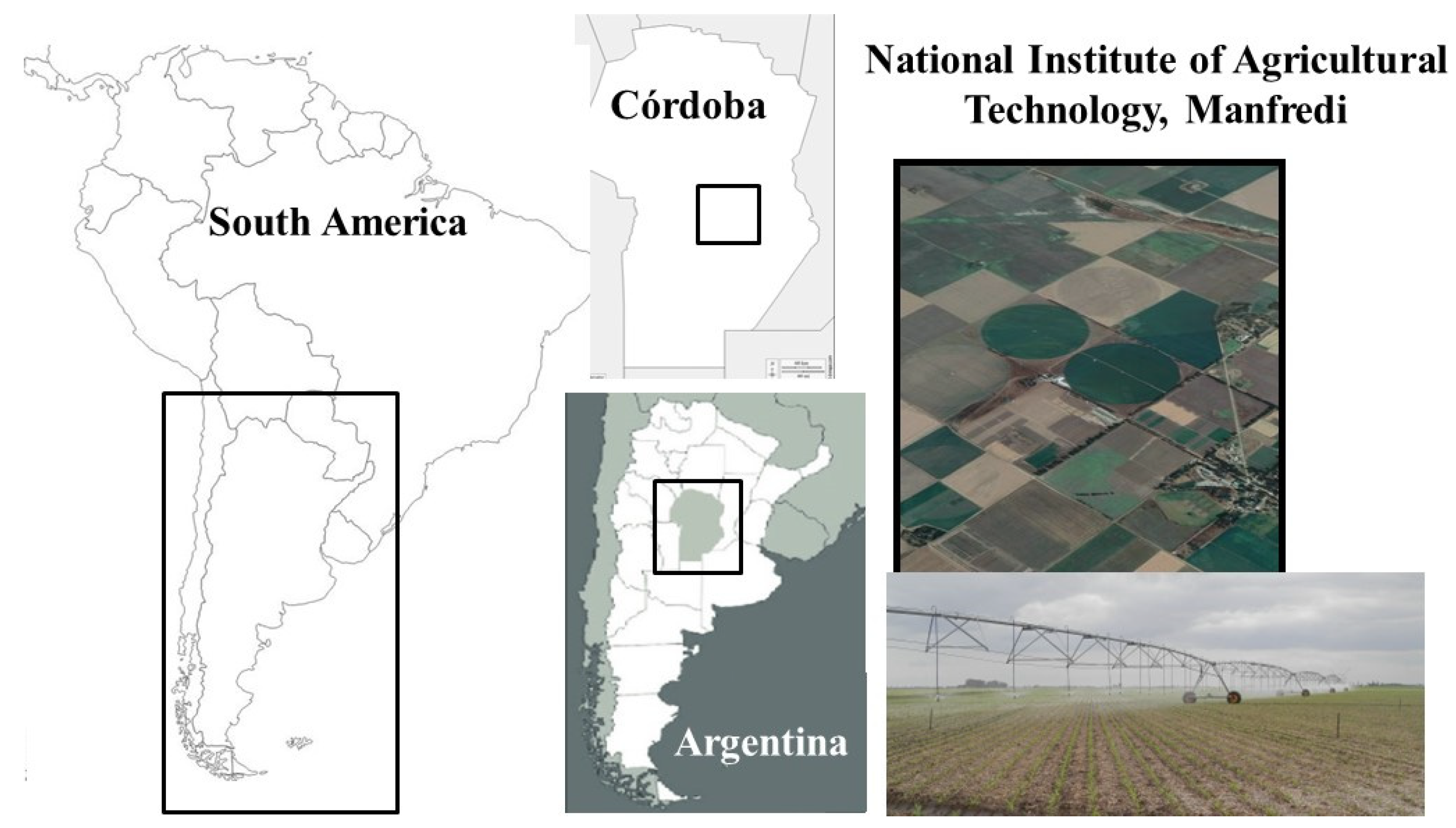
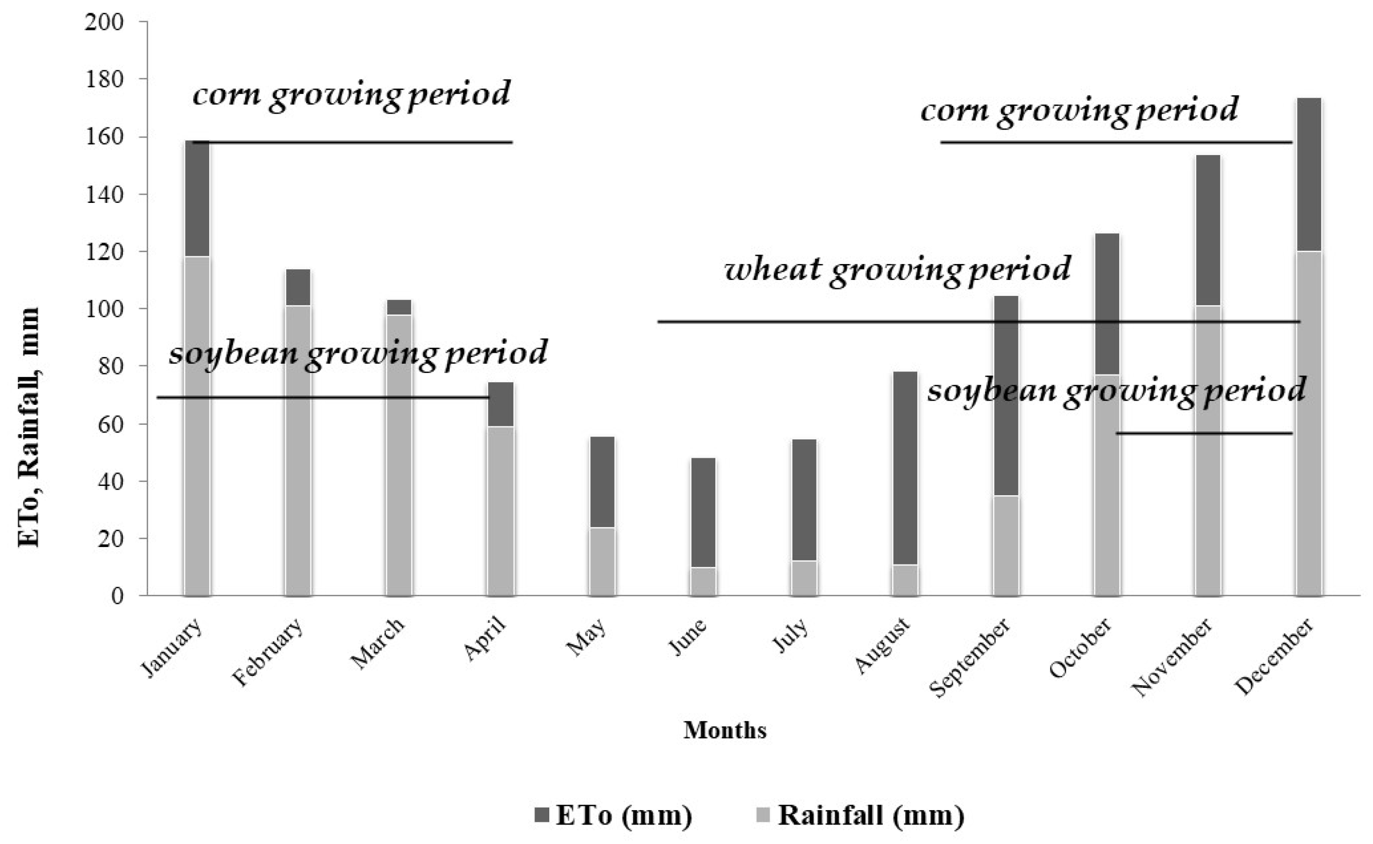
2.1. Edapho-Climatic Characteristics of the Study Area

The study was conducted in the experimental field of the National Institute of Agricultural Technology in Manfredi (Córdoba province, Argentina) (31°49′ S, 63°46′ W, Figure 1) as part of a long-term trial of agricultural crops (from 1996 to present) involving wheat/soybean and corn under a no-tillage system.

The climate is temperate to semiarid [20], with a monsoon hydric regime; mean annual precipitation is 766 mm (1931–2016 series), with 80% concentrated in the warm period (October–March). Mean annual reference evapotranspiration for the same time series is 1300 mm (Figure 2). Mean annual temperature is 16.8 °C, with monthly means for the coldest month (July) and the warmest month (January) of 9.5 °C and 23.4 °C, respectively [21]. Relief and soil characteristics are homogeneous, corresponding to the Oncativo series (Entic Haplustoll), coarse silty, mixed, thermic, silt–loam taxonomic class throughout the profile, with storage capacity from 0.02 m to 2 m in depth and with no physical or chemical restrictions for root development [22].

2.2. Irrigation Equipment

A center pivot system with five 52 m towers and a 42 m overhang that irrigates 27.8 ha was used for the study. The system has 110 sprinklers IWob UP3 (Senninger) spaced between 1.90 and 5.70 m, placed 1.60 m above the ground, with individual pressure regulators (10 PSI). The gross application depth in an irrigation event at 100% speed was 6 mm. Pumping flow was 132 m³ h⁻¹ (water duty of 1.32 L s⁻¹ ha⁻¹), and groundwater sources mainly characterized by: (i) electrical conductivity and total dissolved salts were 1.07 dS m⁻¹ and 683 mg L⁻¹, respectively, and by (ii) sodium adsorption ratio (SAR) and adjusted SAR [23] were 7.5 and 7.9, respectively.

2.3. Application Efficiency

The original equation proposed for evaluating application efficiency (Ea) in stationary sprinkler irrigation systems is Equation (1) [2]:

$$\mathrm{Ea} = \mathrm{Oe} \times \mathrm{Re} \times \mathrm{DUpa}$$

(1)

where Oe: losses due to leaks in pipelines, which are here considered equal to 1; Re: losses due to droplet evaporation and drift; DUpa: distribution uniformity for the percentage of the adequately irrigated area; all of these are the dimensionless components.

The equations used to calculate each of the Ea components were taken from [2]:

$$\mathrm{Re}=0.976+0.005\times \mathrm{ETo}-0.00017\times {\mathrm{ETo}}^2+0.0012\times \mathrm{WS}-\mathrm{CI}\times \left(0.00043\times \mathrm{ETo}+0.00018\times \mathrm{WS}+0.000016\times \mathrm{ETo} \times \mathrm{WS}\right)$$

(2)

where ETo: reference evapotranspiration (mm day⁻¹); WS: wind speed (m s⁻¹); CI: coarseness index proposed by [2]:

$$\mathrm{CI}=0.032\times \frac{{\mathrm{Pa}}^{1.3}}{\mathrm{dn}}$$

(3)

where Pa: sprinkler operating pressure (kPa); dn: nozzle diameter (mm). Equation (3) is valid for 7 ≤ CI ≤ 17; if CI < 7, then CI = 7 and if CI > 17, then CI = 17. The operating pressure used was determined for the pressure regulators of each sprinkler.

$$\mathrm{DUpa}=100+\left(606-24.9\times \mathrm{pa}+0.349\times {\mathrm{pa}}^2-0.00186\times {\mathrm{pa}}^3\right)\left(1-\frac{\mathrm{CUC}}{100}\right)$$

(4)

where pa: percentage of adequately irrigated area; CUC: Christiansen’s uniformity coefficient. In this work, CUC was replaced by the Heermann and Hein coefficient of uniformity (HHCU) since this uniformity indicator is specific for center pivot systems.

$$\mathrm{HHCU}=100\left[1-\frac{{{\displaystyle \sum }}_{1=1}^n\left|V_i-V_{MP}\right|S_i}{{{\displaystyle \sum }}_{i=1}^n{V}_i{S}_i}\right]$$

(5)

where n: number of catch cans; i is a number assigned to identify a particular catch can beginning with i = 1 for the catch can located nearest the pivot point and ending with i = n for the most remote catch can from the pivot point; V_i is the depth collected in the ith catch can (mm); S_i is the distance of the ith collector from the pivot point (m); V_MP is the weighted mean of the amount of water caught (mm).

Weather records were obtained every 5 min from a meteorological station located 1000 m from the irrigation system. To determine Re, the pivot operated during daylight hours, without crop and by applying four irrigation depths (40, 24, 12 and 6 mm). ETo was obtained using the FAO equation [24] and mean or accumulated values corresponding to each irrigation event were calculated.

Two novel features were incorporated into the original equation (Equation (1)), the components of irrigation losses due to partial residue retention (PRR) and leaf interception (LI).

2.4. General Features of the System

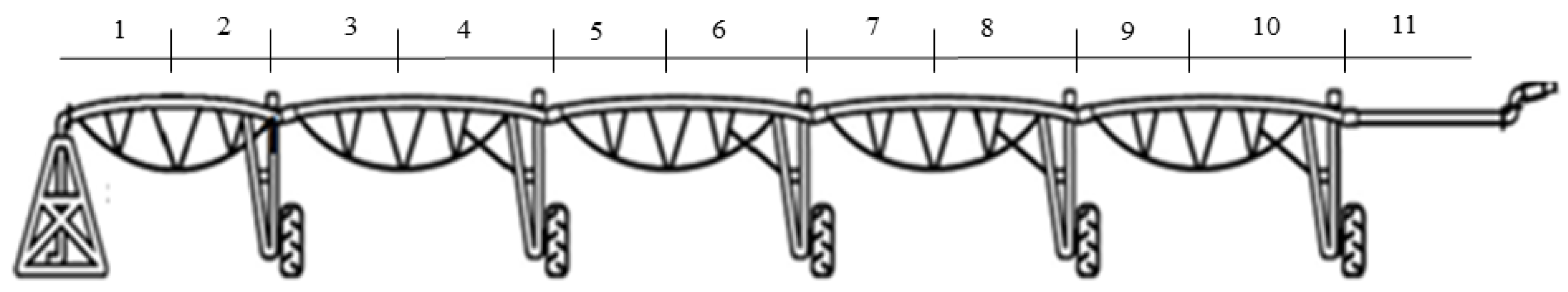
2.4.1. Characterization of the Equipment and Discharged Water

To evaluate the effect of the different water depths of the irrigation system relative to DUpa, the sprinklers with coefficients of variation of flow between 3% and 11% were grouped together, and these groups were called segments (Figure 3). For each segment, the width and length of the wetted area (under no-wind conditions) were determined. The wetted area width was the distance at which droplets land in the central portion of a given segment; this test was performed with the system applying water but not moving. The wetted area length was determined as the sum of the distances between sprinklers included in each segment. Wetting times were also determined and corresponded to each wetted width using four operating speeds (100%, 50%, 25% and 15%). CI (Equation (3)) was calculated with each nozzle included in each segment of the irrigation system.

The theoretical flow of the sprinklers was obtained from the sprinkler package and then confirmed using mechanical flow meters (EX, model: Manu32) located upstream of the pressure regulator. Sprinkler flow was verified by measuring the flow discharged by each sprinkler for 20 min; this procedure was performed in triplicate.

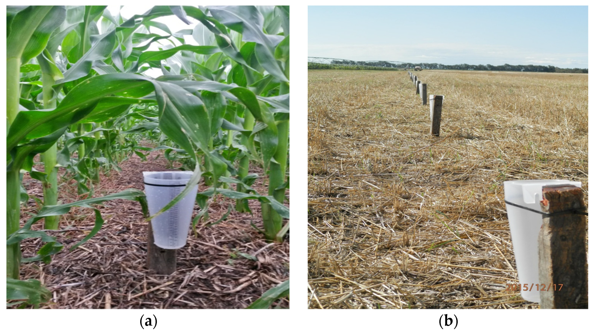
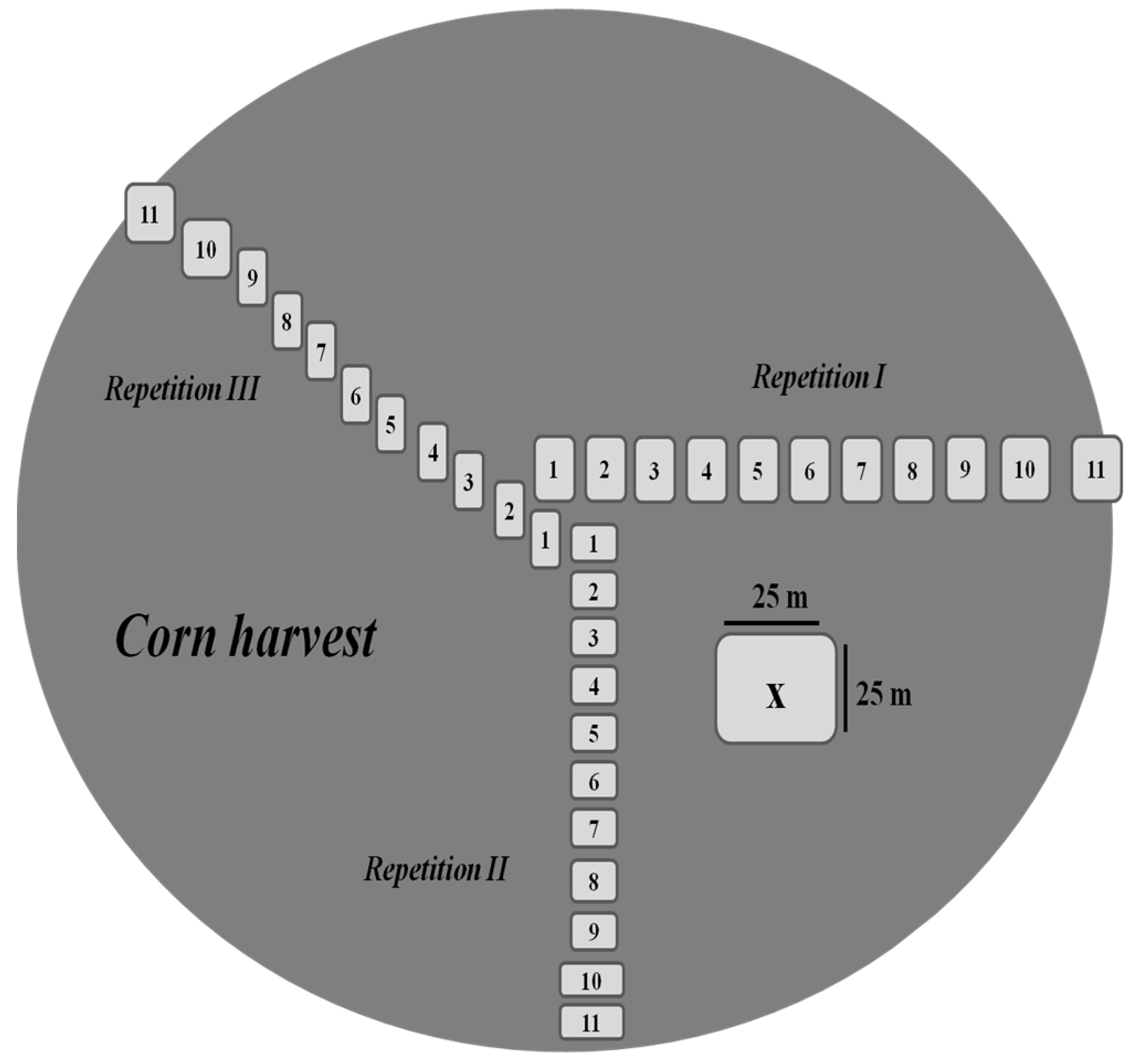
2.4.2. Evaluations Performed and Location of Catch Cans

To determine irrigation uniformity and losses due to interception, measurements were taken in a corn crop (Zea mays, Nidera 734) cultivated under no tillage (6 October 2016) on soybean residue with a 0.52 m row spacing and a density of 4.2 plants per linear meter. Catch cans were distributed following the standards of the American National Standards Institute and American Society of Agricultural Engineers [19]. Catch cans (0.11 m in diameter and 0.22 m in height) were placed at the center of the crop interrow, 0.5 m above the ground and spaced 3 m (Figure 4a). Catch cans were radially arranged along the irrigation equipment, with the first one being at a distance of 20 m to the center of the pivot; thus, more than 99% of the irrigated area was evaluated. Between 8 and 15 catch cans were used per segment, depending on the segment length. A no-crop condition (control) was also evaluated by distributing radially an equal number of catch cans (Figure 4b). To evaluate losses due to direct evaporation, three catch cans were placed 100 m from the end of the equipment to measure the volumes evaporated during the time of application of the different depths used.

2.4.3. Evaluation Times and Position of Sprinklers

Four irrigation depths (Ids) were evaluated (40, 24, 12 and 6 mm) under control conditions and at three vegetative development stages corresponding to the different crop heights (V₄, V₆ and V₁₀), following the scale proposed by [25]. When corn reached the reproductive stage (R₁, 2.8 crop height), a single Id (40 mm) and two conditions were evaluated: with the sprinklers below the canopy (1.6 m from the ground) and sprinklers above the canopy (3 m above the ground) (

Table 1. Depths evaluated in relation to the phenological stage—crop height—and position of sprinklers.

	Speed %	15	25	50	100
	Gross Irrigation Depth, mm	40	24	12	6
		Number of Measurements				Crop Height, m	Sprinkler Height, m
* Phenological stage	Control	3	3	3	3	-	1.6
	V4	1	1	1	1	1.2
	V6	1	1	1	1	1.4
	V10	1	1	1	1	1.55
	R1BC	3	-			2.8
	R1AC	3				2.8	3

* Phenological development stage of corn [25]; V₄: four fully expanded leaves; V₆: six fully expanded leaves; V₁₀: ten fully expanded leaves; R₁BC: reproductive stage with sprinklers below the canopy (1.60 m); R₁AC: reproductive stage with sprinklers above the canopy (3 m). Number of catch cans: 94.

).

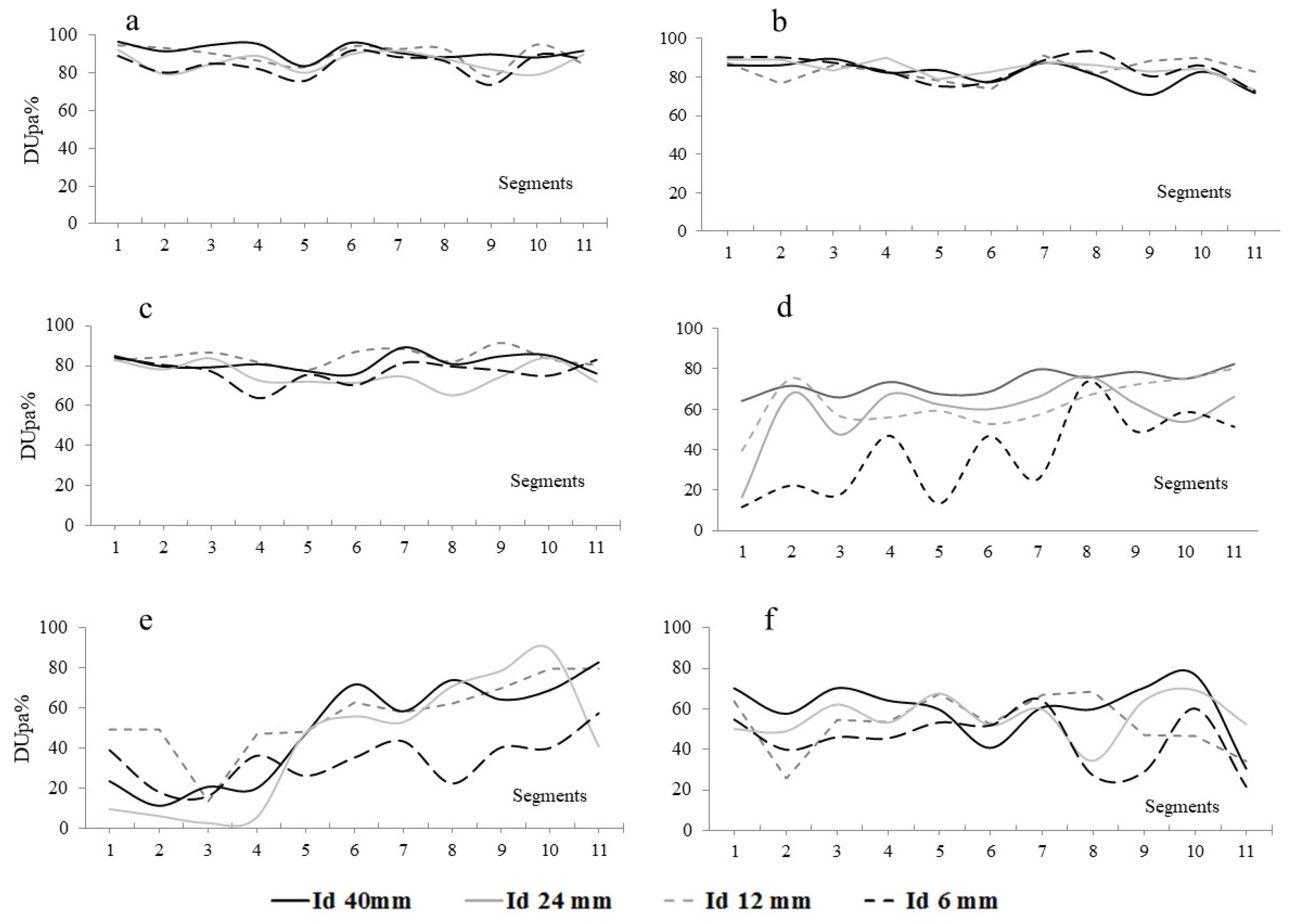
2.4.4. Decrease of Uniformity

With the results of DUpa for each of the phenological stages and depths used, a dimensionless relationship was obtained that represents the relative variations in DUpa with respect to the control:

$$\mathrm{DDUpa}=\frac{{\mathrm{DUpa}}_{\mathrm{y}}-\mathrm{DUpa} \mathrm{Control}}{\mathrm{DUpa} \mathrm{Control}}$$

(6)

where DUpa_y: DUpa for a given crop height (y); DUpa control: DUpa for the control condition (with no crop).

Equation (6) was applied for each segment with the average of the four Ids and an average of the entire equipment.

To confirm the possible effect of sprinkler spacing relative to the uniformity, mean spacing between sprinklers was obtained for each segment and was related to mean DUpa for the four Ids (40, 24, 12 and 6 mm), considering four conditions: (i) Control; (ii) vegetative stage; (iii) reproductive stage with sprinklers below the canopy (R₁BC) and (iv) reproductive stage with sprinklers above the canopy (R₁AC).

2.5. Crop Yield as a Function of Distribution Uniformity

To relate corn yield to DUpa, sampling areas were identified following the method proposed by [26]. Thus, in each of the 11 segments, three 25 m² plots were selected (approximately 210 plants) distributed in three areas or axes of the equipment (considering soil homogeneity), totaling 33 plots (Figure 5). At physiological maturity, all the cobs were harvested and threshed, and the kernels were placed in an oven to constant weight and adjusted at 14.5% of moisture.

2.6. Water Retention in Residues

To determine the irrigation loss component due to residue retention, a trial was conducted on the residues of the rotation involving wheat/soybean and corn; for this purpose, three sites were identified in the central area of each segment. At these sites, metal quadrats (0.25 m²) were placed, and the residue inside the quadrat was cut and removed. Four Ids (6, 12, 24 and 40 mm) were applied, with the sprinklers at a height of 1.6 m, and residues were collected before and after each irrigation event. To determine the initial and final water content, samples were weighed and then placed in an oven at 60 °C to constant weight.

The following parameters were considered: (i) initial retention, water content in residue before irrigation; (ii) partial residue retention (PRR), i.e., amount of water contributed solely by irrigation and (iii) total residue retention (TRR), the sum of (i) and (ii).

2.7. Leaf Interception and Water Redistribution in the Soil

To determine leaf interception, the equations proposed by [4] were considered (Equations (7) and (8)) for rotating, low-pressure sprinklers.

$$\mathrm{Ta}=\left(0.372+0.00313\times \mathrm{d}\right)\times \mathrm{Id}$$

(7)

$$\mathrm{Sa}=\left(0.685-0.00754\times \mathrm{d}\right)\times \mathrm{Id}$$

(8)

where $\mathrm{Ta}$: throughfall (mm); $\mathrm{Sa}$: stem flow, fraction of water intercepted and flowing down the stem to the base of the plant (mm); d: distance between plants along the crop row (mm); Id: irrigation depth (mm).

To validate Ta (Equation (7)), two procedures were used with the crop at R₁: (i) catch can data were analyzed with four Ids (6, 12, 24 and 40 mm), and (ii) soil water content was determined in the interrow (WI) and the row (WR) before and after applying an Id of 40 mm using a precalibrated TDR portable probe with a measurement depth of 0.10 m. A grid pattern of readings (0.1 × 0.1 m; n = 30) was established, both in the crop line and interrow, at three sites per segment of the pivot system, and readings were taken before (50% of field capacity) and 36 h after applying irrigation. The data obtained were used to determine Ta and the coefficient of uniformity of water in the soil (CUs), following the procedure proposed by [26].

The readings obtained in the catch cans and in the WI were correlated with Ta, whereas WR was considered the fraction of water intercepted and flowing through the stem to the base of the plant (Sa). The Sa component was considered equivalent to the intercepted Id, which was obtained as the difference between the Id applied and the collected depth (Dc). The component evaporation from the leaves was not considered due to the characteristics of the corn leaves [27,28,29].

In addition to the validation of Equations (7) and (8), other regressions were performed that included different crop heights (1.20, 1.40, 1.55 and 2.80 m); thus, a new height component was obtained:

$$\mathrm{H}=h_a-(h_p-h_c)$$

(9)

where H: vertical height (m); $h_a:$ sprinkler height from the ground (m); $h_{p }:$ plant height from the ground to the base of the stem where the last expanded leaf is inserted (m); $h_c:$ height of catch can from the ground to the upper border (0.50 m).

2.8. Statistical Analysis

DUpa was statistically analyzed using a one-way analysis of variance, with the factors being the Id and the phenological stages, including the control. Means were compared using Fisher’s LSD test, with a significance level of 0.05 [30]. The variability of the samples collected in the different trials was analyzed using the standard deviation and the coefficient of variation. To determine the components LI and PRR, linear and multiple regression analyses were conducted, including the principal variables (initial and final residue water content, dry matter, irrigation intensity of segments, Id). Crop yield and DUpa were also subjected to linear and multiple regressions. All the analyses were performed using Infostat statistical software [31].

3. Results and Discussion

3.1. Flow and Irrigation Intensity of Segments

Eleven segments were determined. The measured (actual) flows of each segment were between 11% and 18% higher than the designed (theoretical) ones, whereas the CV of the initial segment was much higher than that of the final segments (

Table 2. Theoretical and actual mean flows (m³ h⁻¹) for each segment and their corresponding coefficients of variation (CV).

Segments	Designed Flow		Actual Flow		Actual Flow/Designed Flow Ratio
	m3 h−1	CV	m3 h−1	CV
1	0.27	36.16	0.3	44.47	1.11
2	0.63	16.89	0.72	17.91	1.14
3	1.08	11.48	1.28	12.16	1.19
4	0.77	12.33	0.91	10.29	1.18
5	1.08	11.74	1.27	11.74	1.18
6	1.4	7.28	1.63	7.28	1.16
7	1.59	4.87	1.87	4.87	1.18
8	1.72	4.76	1.99	4.76	1.16
9	2.00	4.18	2.21	4.18	1.11
10	2.00	5.08	2.21	5.08	1.11
11	2.04	15.75	2.14	4.35	1.05

).

Wetted width showed an increasing trend in the initial segments (1 to 3), reaching 14 and 15 m in the final segments (

Table 3. Width, length, irrigation intensity, wetting time and coarseness index for the different segments of the irrigation system and four operating speeds (%).

					Operating Speeds
					100%	50%	25%	15%
Segments	Wetted Width, m	Wetted Length, m	Average Application Rate, mm h−1	CI	Wetting Time, Minutes
1	8.7	24.1	5.7	7	51	98	349	482
2	11.2	26.8	12.0	7	36	58	142	193
3	14.5	34.2	15.4	7	17	32	65	111
4	13.7	23.9	25.0	7	19	32	74	108
5	14.3	55.2	32.1	7	14	25	56	83
6	14.3	25.9	39.6	7	10	17	42	52
7	14.5	29.4	48.3	7	8	15	30	55
8	14.5	24.6	50.2	7	8	14	34	47
9	14.7	23.9	56.7	7	7	13	32	41
10	14.5	17.3	79.4	7	7	11	25	43
11	15.1	12.3	77.4	7	5	8	17	31

CI: coarseness index, dimensionless.

), in agreement with the theoretical wetted diameter of sprinklers. Wetted length depends on the number of sprinklers grouped; segment 5 is the greatest (55.2 m, Table 3), with 20 sprinklers grouped. Likewise, the coarseness indices (CI) were 7 for all the segments since CI was lower than 7 (Equation (3)). Irrigation intensity increased from 5.7 to 77.4 mm h⁻¹ in the successive segments (Table 3), which allowed us to represent changes in irrigation intensity along the center pivot system.

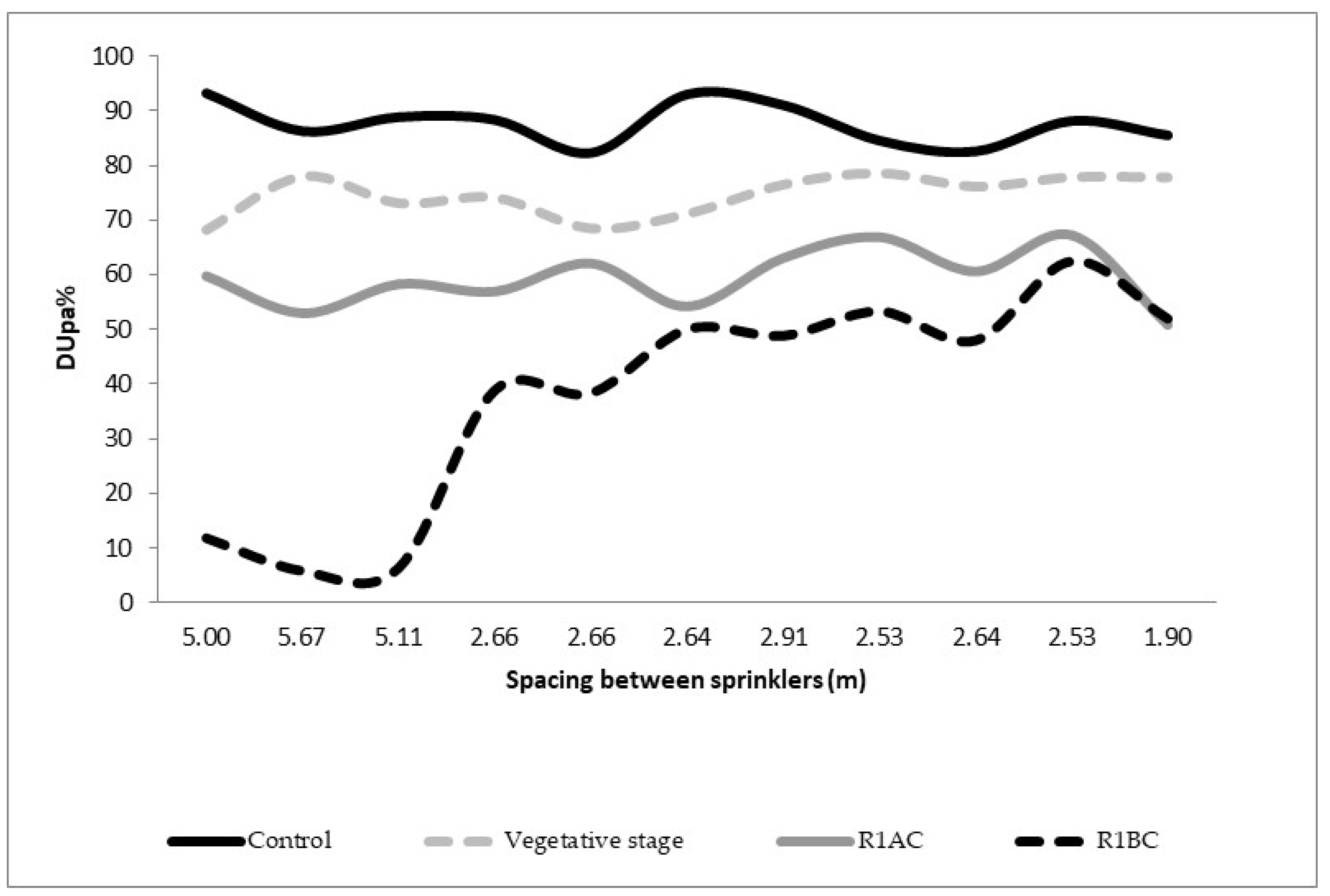
3.2. Distribution Uniformity

Mean DUpa (control) calculated with pa other than 80% differed from mean HHCU (

Table 4. Mean HHCU and DUpa of the four Ids used in the control condition.

			Segments
		1	2	3	4	5	6	7	8	9	10	11
pa	HHCU, %	93.6	86.9	89.4	88.9	83.0	93.4	91.5	85.2	83.3	88.7	86.1
70	DUpa (%)	96.8	91.5	93.1	92.8	89.0	95.7	94.5	90.4	89.2	92.6	91.0
75		94.1	89.1	91.2	90.7	85.9	94.5	92.9	87.7	86.1	90.6	88.5
80		93.4	86.3	88.9	88.3	82.2	93.1	91.1	84.5	82.5	88.1	85.5
85		92.5	82.8	86.0	85.4	77.7	91.3	88.8	80.6	78.1	85.1	81.8
90		91.5	78.5	82.5	81.7	72.2	89.1	86.0	75.7	72.6	81.4	77.2

HHCU, Heermmann and Hein coefficient of uniformity; DUpa, distribution uniformity; Id, irrigation depth; pa, percentage of adequately irrigated area.

), in agreement with the equation proposed by Keller and Bliesner [2]. With pa of 80%, DUpa and HHCU were similar and regarded as very good for sprinkler irrigation according to [19], whereas with pa > 80%, segments 5 and 9 had DUpa below 80%, the threshold recommended for sprinkler irrigation. The values obtained allowed us to adapt the DUpa equation proposed by [2] using HHCU.

Conceptually, the DUpa equation means that for a given pa, the deficit between the desired net Id and the Id effectively stored in the soil increases with decreasing uniformity [2]. With a pa of 80%, DUpa is similar to HHCU, indicating the most adequately irrigated area. As pa decreases, a lower extra Id is necessary, but the proportion of under-irrigated area increases; this depends both on the sensitivity to water deficit and the economic value of the crop used [32].

Thus, to compare the different DUpa values calculated with the different Ids, position of sprinklers and phenological stages, a pa of 80% was used. The control condition (Figure 6a) indicates the water distribution model without crop, which presented values regarded as good to very good for the four Ids analyzed, according to the classification of [19]. This condition represents the optimum water distribution and can be used for comparison with respect to the DUpa obtained in the presence of the crop. The high DUpa obtained may be due to a correct design of the sprinkler package and wind speeds <3 m s⁻¹ during the trials, among other factors.

When the crop reached a height of 1.20 m (V₄, Figure 6b), interference of the applied water started, which was evidenced in a decrease of DUpa of 0.5% to 10.8% with respect to the control, considering all the Ids applied and all the segments. When the crop was 1.40 m in height (V₆), DUpa continued to decrease (between 6.9% and 12% for all the Ids and segments) up to values between 60% and 70% for segments 4 and 6 using an Id of 6 and 12 mm, respectively (Figure 6c). Similar uniformity (55%) was obtained in a 0.5 m tall corn crop irrigated with a center pivot [33].

When sprinklers were below the canopy (V₁₀, 1.55 m), the decrease in DUpa with respect to the control increased, reaching between 20% and 40% for segments 1, 2, 3, 5 and 7 (Figure 6d). In turn, at the same stage, the lowest DUpa was obtained with the lowest Id applied (100%), with variability between segments being also very high.

When the crop was 2.80 m in height (R₁), DUpa was obtained under two operating conditions: sprinklers at 1.60 m (R₁BC, below the canopy) and 3.2 m above the ground (R₁AC, above the canopy). Mean DUpa decreased between 52.5% and 67% with respect to the control with the sprinklers below the canopy (Figure 6e), the highest decrease of all the tests, whereas the elevation of sprinklers improved DUpa, with a reduction of 34.6% to 47% with respect to the control (Figure 6f). These results differ from those reported by [34], who evaluated LDN (low drift nozzle–Senninger) sprinklers at different positions and concluded that the highest position increased the drift loss of the sprinkled droplets. These contrasting results were due to wind speeds: 3 m s⁻¹ in the present work and 10 m s⁻¹ in the work of [34]. However, no differences in uniformity were found in a study evaluating impact sprinklers above and below the canopy in alfalfa [35]; this result is explained by the planophile orientation and trifoliate compound leaves of alfalfa, unlike corn leaves, which are linear to linear–lanceolate simple leaves.

To evaluate the influence of sprinkler spacing on uniformity, the mean spacing of each segment vs. mean DUpa was represented for all the Ids of the control, vegetative stages (V₄, V₆ and V₁₀) and reproductive stages with sprinklers below the canopy (R₁BC) and above the canopy (R₁AC) (Figure 7). While DUpa decreased at the vegetative stage and at R₁AC, this result was not due to spacing but to canopy interference since the reduction was similar for all spacings. By contrast, at R₁BC DUpa dropped abruptly with spacings between 5 and 5.1 m (Figure 7). The greatest reduction of DUpa occurred in the first segments, where sprinkler spacing was greater. In this situation, with a 5.2 m spacing and corn planted at 0.52 m between rows, 10 crop lines or 20 corn plants (sowing density of 4.2 plants per linear meter) interfered with the droplet trajectory, causing great interference [36,37]. To obtain the highest DUpa and, in turn, the smallest difference between curves that represent the phenological stages, the optimum sprinkler spacing was 2.5 m (Figure 7).

The analysis of DUpa results with respect to Ids showed no significant differences for the control condition or V₄, (

Table 5. Average of distribution uniformity (DUpa) of all segments considering the different irrigation depths at each of the phenological stages and in the control condition.

	Irrigation Depth (Id, mm)
	40		24		12		6
* Phenological Stage	DUpa, %
	Average	CV	Average	CV	Average	CV	Average	CV
Control	0.90 C b	13.3	0.91 C b	15.7	0.85 C b	20.1	0.85 C b	11.8
V4	0.84 C a	6.9	0.82 C a	7.6	0.84 C a	6	0.84 C a	8.1
V6	0.84 C c	4.5	0.81 C cb	5.3	0.76 C ab	7.8	0.76 C ab	7.5
V10	0.70 B b	16.3	0.59 B ab	32.8	0.59 B ab	27.3	0.45 B a	56.6
R1AC	0.66 B b	26.3	0.65 B b	22.8	0.65 B b	18.1	0.60 B a	31.4
R1BC	0.51 A b	56.8	0.46 A ab	72.6	0.40 A ab	87.5	0.32 A a	166.4

* Phenological stage of corn according to [25]. Control: area of the irrigated circle with no crop; V₄: vegetative stage with four fully expanded leaves; V₆: vegetative stage with six fully expanded leaves; V₁₀: vegetative stage with ten fully expanded leaves; R₁AC: reproductive stage and sprinklers above (3.20 m) the crop canopy; R₁BC: reproductive stage and sprinklers below (1.60 m) the crop canopy; different uppercase letters (A, B, C) among phenological stages indicate significant differences (p ≤ 0.005) according to the LSD test; significant lower case letters (a, b, c) between Ids indicate significant differences (p ≤ 0.005) according to the LSD test.

). These DUpa values were good to excellent [19]. At V₆, a significant reduction (p ≤ 0.05) in DUpa was detected (between 50% and 100% with respect to 15%), whereas at V₁₀ and R₁AC, only Id 6 mm had a significant reduction (p ≤ 0.05) with respect to the remaining depths. At R₁BC, a significant reduction (p ≤ 0.05) in DUpa between 100% (6 mm) and 15% (40 mm, Table 5) was recorded. These results indicate that at advanced growth stages, the highest Id performed better regarding uniformity. Thus, using 40 mm at advanced growth stages can be considered a management criterion.

Distance between sprinklers and crop canopy had effects on uniformity since DUpa was significantly reduced (p ≤ 0.05) from V₆ and at all the Ids applied (Table 5). This result is explained by the interference of plants in the droplet trajectory; indeed, this interference hinders an appropriate overlap as the distance between the canopy and the sprinkler decreases [8]. According to these authors, the magnitude of the irrigation losses depends on the storage capacity of leaves (canopy) and the amount of energy available for evapotranspiration, with losses ranging between 7% and 10%.

The highest decrease occurred after V₁₀, with the lowest values being recorded at R₁BC (Figure 6); this behavior was independent of the rates applied. Phenological stages V₄ and V₆ had the lowest DUpa reductions, between 6% and 12% for both stages.

To predict the decrease in the distribution uniformity as a function of phenological stage, a quadratic regression equation was generated using the average DDUpa for all the segments, with a significance level of p ≤ 0.0001:

$$\mathrm{DDUpa}=-0.01\times {\mathrm{de}}^2$$

(10)

where de: days after crop emergence. This equation is valid for >30 days.

3.3. Losses Due to Evaporation and Drift (Re)

The component Re had low variability and little effect on total water loss, even with very high ETo and wind speed (

Table 6. Losses due to droplet evaporation and drift (Re).

Start Time, h	Irrigation Time, h	ETo, mm h−1	Wind Speed, m s−1	Pivot Operating Speed, %	Re
19:00 p.m.	7.50	2.6	1.80	15	0.98
21:00 p.m.	5.80	7.5	3.17	25	0.98
11:00 a.m.	1.80	9.4	1.39	50	0.97
08:00 a.m.	0.85	6.1	3.00	100	0.98

Coarseness index (CI) was lower than 7 in all the pivot segments. ETo: reference evapotranspiration.

). This result was due to the low wind drift (speed ≤ 3 m s⁻¹) and to the similarity between the average of the evaporation losses in the three catch cans placed at the base of the pivot (2%) and the losses calculated through the Re equation. However, wind speed was found to be the variable that best explained evaporation and drift losses, with abrupt changes in wind speed and direction also affecting those losses [38].

The sprinkler used in the test has a grooved deflector plate that, coupled with a wobbling action, emits droplets of 2 to 4 mm in diameter (a situation that is not considered in Equation (6)); these droplets are barely sensitive to the action of wind and evaporation [37]. The authors also evaluated a sprinkler with two types of plate, smooth and coarse serrated (droplet size of 0.3 to 5 mm), and determined evaporation and drift loss of 0.7 to 1.4% for a smooth plate and 0.4 to 0.6% for a serrated plate at equal operating pressure to those used in this work but under higher wind speed conditions (6 m s⁻¹) [39].

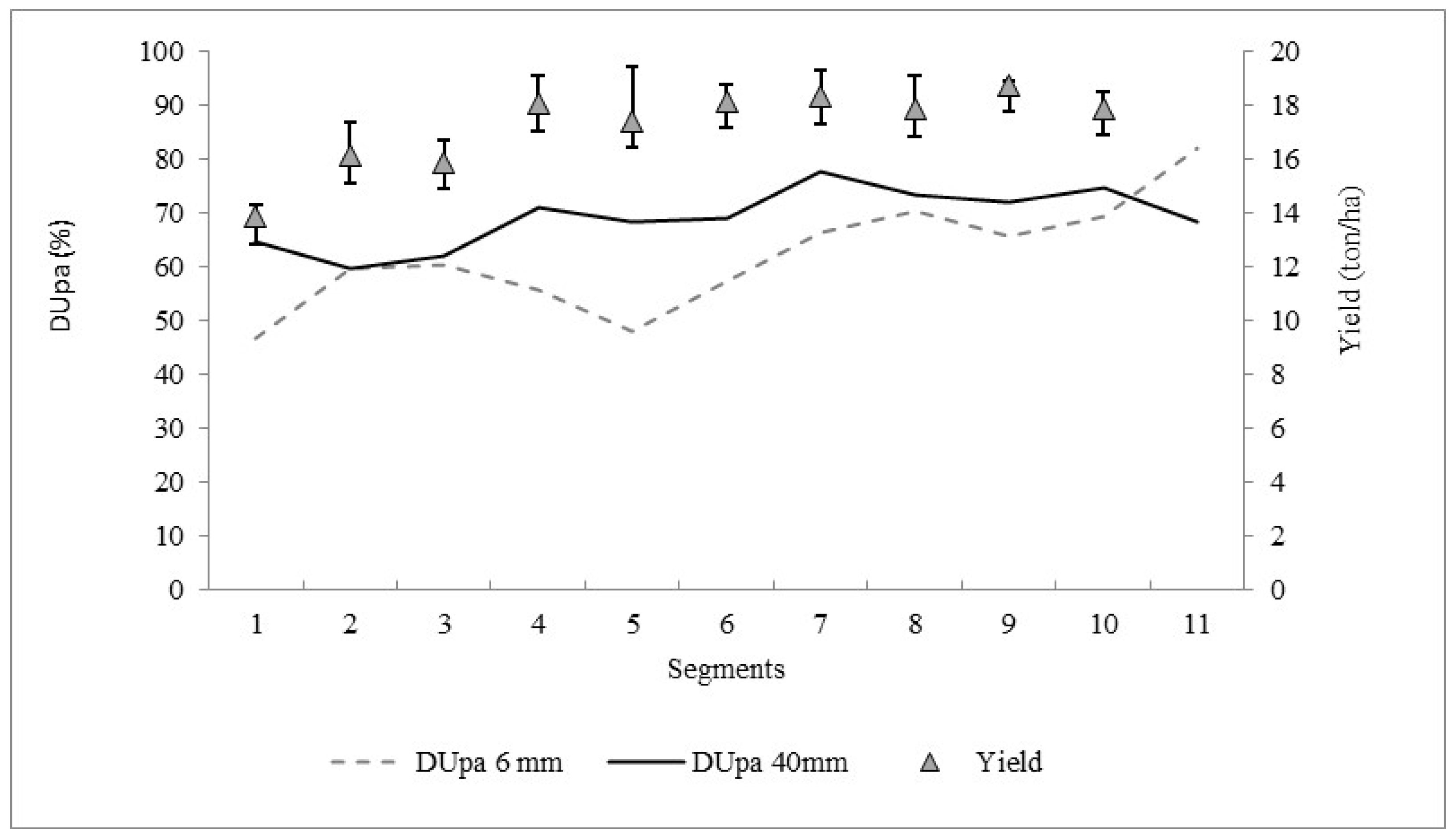
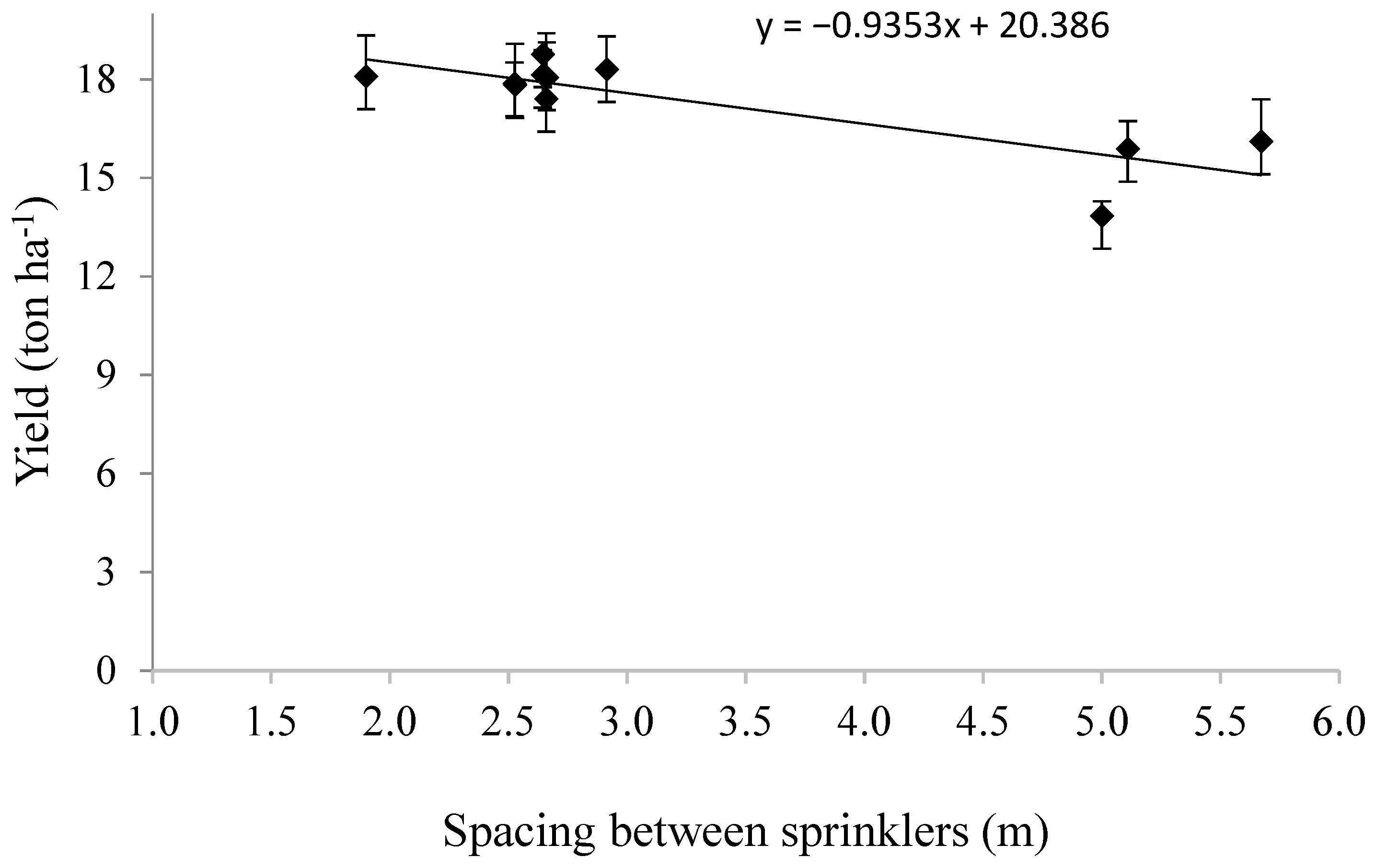
3.4. Crop Yield vs. Distribution Uniformity

Irrigation amounted to 320 mm during the crop cycle, and crop yield was between 14 and 18 ton ha⁻¹. The lowest yields corresponded to the initial segments (1 to 3), where uniformity was lower (regardless of the Id), whereas yield became stable at 18 ton ha⁻¹ for the remaining segments (Figure 8). Difference in yield (4 ton ha⁻¹) is related to the lower uniformity of the initial segments, with sprinklers being spaced at 5 m, since the Id was similar in all the segments. A study involving sprinklers above the corn crop and similar spacing to that used in this work found yield losses of 2.5 ton ha⁻¹ in the central row with respect to the rows closer to the sprinklers [37]. By contrast, studies involving wheat [38] and sugar beet [40] found that yield is not always affected by reduced uniformity. This finding was attributed to an improvement in uniformity after successive irrigation events, to the interception and redistribution of water in the canopy, the redistribution of water in the soil and root development. A linear decrease in yields with respect to the increase in sprinkler spacing (spacing ranging between 1.9 and 5.7 m) was found (Figure 9).

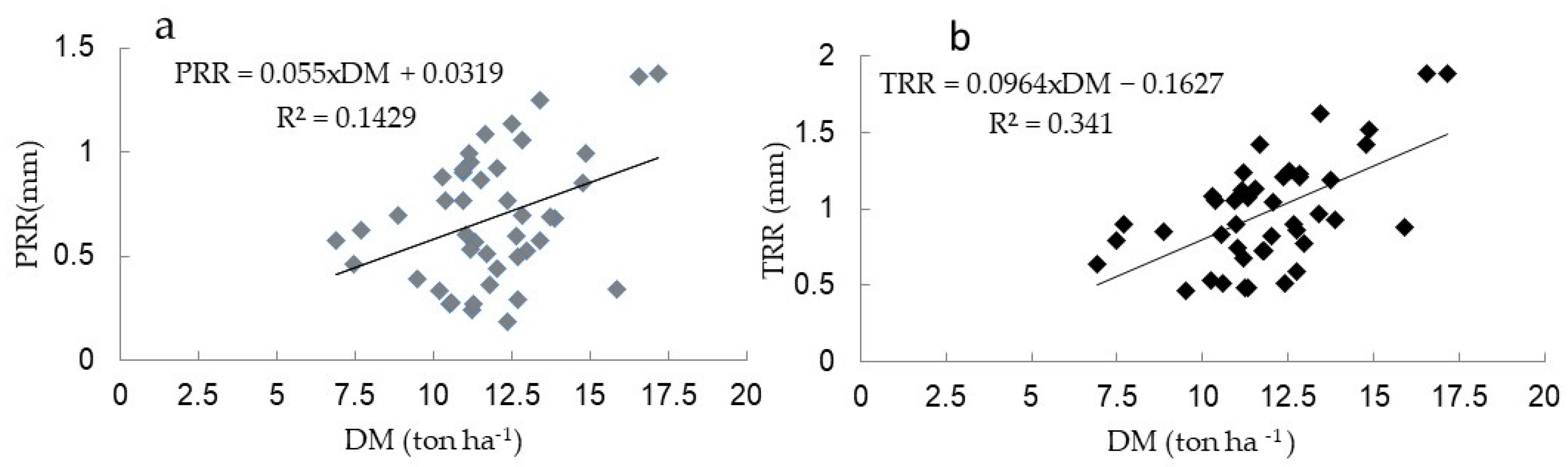
3.5. Water Retention by Residues

The amount of irrigation retained by harvest residues was explained significantly (p ≤ 0.0001) by both the different application Ids and the amount of dry matter residue (Equation (11)). On the other hand, the analysis of the irrigation intensity of segments and the initial water content in the residue showed no significant relationship with water retention:

$$\mathrm{PRR}=0.44+0.05\times \mathrm{DM}-0.02\times \mathrm{Id}$$

(11)

where PRR: partial residue retention generated exclusively by the irrigation event (mm); DM: dry matter (ton ha⁻¹) and Id: irrigation depth applied (mm). Each of the terms had a significance level of p ≤ 0.0001.

Both partial and total residue retention increased with the increase in dry matter (Figure 10a,b); however, there was a greater variability in partial (PRR) than in total (TRR) for a given amount of dry matter (CV of 45% and 35%, respectively).

Water retained in residue increased with the increase in dry matter up to a limit close to 2 mm in TRR (Figure 10b) and 1.5 mm in PRR (Figure 10a), and according to Equation (11), only 5% of the total amount of dry matter is retained. The maximum retained irrigation may represent an important loss relative to the Id applied, e.g., 25% if 6 mm is applied. These retention levels were reached with high amounts of dry matter (15 ton ha⁻¹), a condition that can occur in no-tillage crops that are irrigated [41]. On the other hand, residue decomposition increases under high temperature and relative humidity [42]. The opposite occurs in cool climates, where residues accumulate due to the low mineralization rate [43]. The relationship between water retained in the residue and dry matter was found to respond to a quadratic equation, with the slope becoming less steep as dry matter increased [17]. The authors attributed this behavior to the overlap of residue layers and indicated that when water is applied (irrigation or rain), the droplets reaching the surface of the residue are retained by adhesion and cohesion forces until they reach a given thickness in which gravity forces act. If irrigation continues to be applied, retention in the upper residue layer will be constant since the new droplets displace those already present to lower residue layers. In corn residues, as decomposition increases, macroporosity rises, thereby increasing the water retention capacity of the residue [14]. Thus, the proportion of corn in the residue increases with increasing porosity (67.93% cobs, 86% leaves, 58.51 stalks) [44], and so does the capacity to accumulate water, which then evaporates depending on wind, temperature and radiation conditions [16], up to a maximum amount of dry matter.

On the other hand, the behavior of PRR at the different Ids applied was opposite to that of dry matter since water retained was lower at higher depths (Figure 11a,b). Thus, the maximum PRR and TRR (1.5 and 2 mm) were recorded at the lowest depths, whereas Ids higher than 25 mm yielded PRR and TRR lower than 0.5 and 1 mm, respectively.

For the 40 and 6 mm Ids, with the same dry matter present in the field, PRR accounted for different loss percentages (5% and 50%, respectively). These losses can be reduced by irrigation management by applying higher Ids.

3.6. Leaf Interception and Water Redistribution in the Soil

3.6.1. Throughfall (Ta) and Stemflow (Sa)

Throughfall was directly related to both the depth collected and differences in height of sprinklers, catch cans and plants (H, Equation (9)). The best fit was obtained with a quadratic equation (each of the terms had a significance level of p ≤ 0.0001):

$$\mathrm{Ta}=-1.28-1.79\times \mathrm{H}+1.82\times \mathrm{Dc}-0.04\times {\mathrm{Dc}}^2$$

(12)

where Dc: depth collected (mm); H: vertical distance between sprinkler height and catch can height (m). To make the application of Equation (12) easier, and considering that Dc estimation requires field measurements, a regression was performed to determine this variable (each of the terms had a significance level of p ≤ 0.0001):

$$\mathrm{Dc}=2.83\times {10}^{0.05\times \mathrm{Id}}$$

(13)

where Dc: depth collected (mm) and Id: depth applied (mm) and

$$\mathrm{Sa}=-1.47-2.07\times \mathrm{H}+2.09\times \mathrm{Dc}-0.05\times {\mathrm{Dc}}^2$$

(14)

where Dc: depth collected (mm); H: vertical distance between sprinkler height and catch can height (m).

Stemflow had similar behavior to that of throughfall, with the participation of Dc and H (each of the terms had a significance of p ≤ 0.0001). The equations proposed by [4] did not have an appropriate fit because we used i-Wob sprinklers (rotating, oscillating and low-pressure), whereas [4] used high-impact, high-pressure sprinklers. Additionally, the distances between sprinklers and crop canopy at different stages were also different. For this reason, we incorporated a new variable (H, Equation (9)) that considers this aspect and resulted in a better fit of Ta and Sa. H allows us to evaluate pivot systems with sprinklers located at different heights.

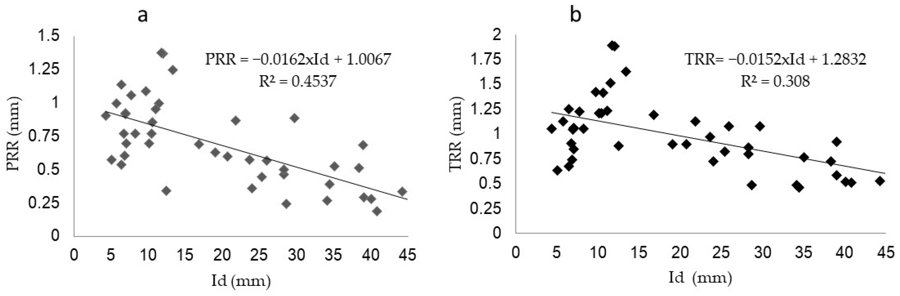
3.6.2. Water Redistribution in the Soil

The mean depth collected and water infiltrated in the interrow were similar but different from the mean Ta obtained with Equation (12), whereas Sa, WI and WR differed from one another. However, the sum of the different components involved in the interrow and row was approximately equal to the depth applied (

Table 7. Means (mm) of the measured irrigation components estimated both in the crop line and in the interrow, relative to the irrigation depth applied.

Interrow (mm)		Crop Line (mm)		Depth (mm)
WI	12	WR	17	40 *
Dc	12	Intercepted Id	28
Ta	17	Sa	20

* The sum of the variables in each row is approximately the same as the depth applied (40 mm). WI: water infiltrated in the interrow (mm); WR: water infiltrated in the crop row (mm); Ta: Throughfall (mm); Intercepted Id (mm); Dc: Depth collected (mm) and Sa: Stemflow (mm).

). The higher water content in the crop line than in the interrow is explained by the fact that erectophile leaves (e.g., corn) have a leaf insertion angle with respect to the stalk smaller than 90°, which causes water retention at this insertion point and a flow to the base of the stem of up to 50% of the total amount of irrigation applied [6]. An increase in water content in the crop line was also reported in a study that measured water in the soil with TDR sensors; the finding was attributed to the preferential flow through the stem [45]. Likewise, water content was found to be higher in the 0.20 m around the crop plant and in the first 0.10 m in depth of the soil profile compared with the water content in the interrow [46]. On the other hand, a preferential flow under the crop corn line was found [47]; the authors estimated that more than 40% of water received from an incident rainfall would be due to stemflow.

The difference between the intercepted Id and the infiltrated water in the crop row (WR), corresponding to an Id of 40 mm (Table 7), might be due to some of the following: (a) water evaporated from the leaves. A work conducted in corn crop using spray sprinklers similar to those used in this trial reported losses of 1 mm [37]. Likewise, losses of up to 2.2 mm for days of high evapotranspiration were reported [8]; (b) water retained by crop residue. In this work, the maximum retention was 2 mm; (c) water redistributed below the soil depth evaluated. To estimate this, if we consider that the sum of (a) and (b) was about 4 mm, and that the difference between intercepted Id and WR was 9 mm, then the difference (5 mm) would have redistributed below 0.1 m.

Considerable differences were detected between mean DUpa (considering depths and segments) and CUs. At R₁AC, values were 53.4% and 97.5%, respectively, whereas at R₁BC, they were 34.8% and 97%, respectively. Redistribution was very important and independent of the water application mode and may be explained by the soil texture and hydraulic conductivity associated with water content before irrigation events [48]. CUs above 90% were found in soil of volcanic origin and in soil of sandy loam texture, even when irrigation was performed with uniformity below 60% [49]. Likewise, a study relating the uniformity of the aerial part to that of the soil in a corn crop under stationary sprinkler irrigation found high water uniformity in the soil (approximately 95%) compared with the uniformity of irrigation application (between 50% and 90%) [50]. Our results agree with those findings, with DUpa and CUs for fully expanded corn crop of 40% and 90%, respectively.

3.7. Revised Equation of Application Efficiency

We propose a new equation that considers the different components:

$$\mathrm{REa}=\mathrm{Re} \times {\mathrm{DUpa}}_{\mathrm{aj}}\times \mathrm{PRR} \times \mathrm{LI}$$

(15)

where REa: revised equation of application efficiency; Re: losses due to evaporation and drift (Equation (2)) and DUpa_aj: DUpa adjusted according to days after crop emergence, leading to:

$${\mathrm{DUpa}}_{\mathrm{aj}}=\mathrm{DUpa} \left(\mathrm{control}\right)\times \left[1-\left(-\frac{\mathrm{DDUpa}}{100}\right)\right]$$

(16)

PRR: losses due to partial residue retention obtained from Equation (11) and divided by Id (mm) to make it a dimensionless loss fraction, leading to:

$$\mathrm{PRR}=1-\left(\frac{0.44+0.05\times \mathrm{MS}}{\mathrm{Id}}-0.02\right)$$

(17)

LI: losses through leaf interception, obtained by summing the components Ta (Equation (12)) and Sa (Equation (14)), replacing and rearranging terms of Equation (13), and dividing by depth (mm) to make it dimensionless, leading to:

$$\mathrm{LI}=1-(\frac{2.75+\mathrm{Id}+3.86\times \mathrm{H}-11.065{ \mathrm{e}}^{0.05\times \mathrm{Id}}+0.721{ \mathrm{e}}^{0.1\times \mathrm{Id}}}{\mathrm{Id}})$$

(18)

The results for the revised equation of application efficiency are presented in

Table 8. Application efficiency obtained using the revised equation including new components of irrigated water loss obtained from experimental results.

eId, mm	Dc, mm	de	H, m	DM, ton/ha	PRR	LI	DUpa	DDUpa, %	DUpaaj	Re	REa, %
10	4.7	30	1	10	0.926	0.967	0.85	−9	0.77	0.98	68
10	4.7	30	1	15	0.901	0.967	0.85	−9	0.77	0.98	66
10	4.7	30	1	20	0.876	0.967	0.85	−9	0.77	0.98	64
15	6.0	40	1	10	0.957	0.906	0.85	−16	0.71	0.98	61
15	6.0	40	1	15	0.941	0.906	0.85	−16	0.71	0.98	60
15	6.0	40	1	20	0.924	0.906	0.85	−16	0.71	0.98	59
25	9.9	50	1	10	0.982	0.929	0.85	−25	0.64	0.98	57
25	9.9	50	1	15	0.972	0.929	0.85	−25	0.64	0.98	56
25	9.9	50	1	20	0.962	0.929	0.85	−25	0.64	0.98	56
40	20.9	70	1	10	0.997	0.895	0.85	−49	0.43	0.98	38
40	20.9	70	1	15	0.990	0.895	0.85	−49	0.43	0.98	38
40	20.9	70	1	20	0.984	0.895	0.85	−49	0.43	0.98	37

Dc: depth collected; de: days after emergence; H: vertical distance, (Equation (9)); DM: dry matter of residue; PRR: partial irrigation water retention in residue (Equation (17)); LI: leaf interception (Equation (18)); DUpa: uniformity of distribution for an adequately irrigated area (Equation (4)); DDUpa: decrease of DUpa (Equation (10)); DUpaaj: adjusted distribution uniformity (Equation (16)); Re: losses due to evaporation and drift (Equation (2)); REa: revised equation of application efficiency (Equation (15)).

, with the irrigation depth and dry matter of residue used in this experiment. Values below or above these ranges can determine any inconsistent results of a component, particularly LI. In Equation (18), this new component (LI) has a minimum of 0.895 and a maximum of 0.967, i.e., between 3.3% and 10.5% of losses of the applied irrigation. LI incorporates both throughflow and stemflow and is adjusted for corn. While experiments involving other crops are necessary to validate this equation, the variables included (H and Id) are easily obtained since the mathematical expression combines linear and exponential terms. The component PRR is universal and can be applied to no-tillage systems that include the rotation of gramineous and leguminous species. Dry matter of residue must be measured before the irrigation campaign; this measurement is an easy procedure that only requires an oven for drying the harvest residue. These values may remain constant in long-term rotation of agricultural crops [51] and can be obtained by government research agencies at the regional level.

The DUpa equation can be applied to a control condition, which can be evaluated using the standards of [19]. The pivot system can be evaluated at least once a year to confirm the functioning of sprinklers. To include the effects of a tall-growing crop (e.g., corn) on the uniformity of distribution, we propose an adjusted equation that includes days after emergence, a measure that is easily obtained by farmers. The REa obtained with the new equation are relatively low, with DUpa_aj being the component that most widely affected application efficiency (Table 8). If the texture of the horizontal surface profile allows water redistribution in the soil (CUs ≥ 90%), then DDUpa might not be considered (i.e., it has a value of 0), DUpa_aj = DUpa, and therefore, REa increases considerably.

4. Conclusions

The application efficiency equation of Keller and Bliesner was adapted for use with a center pivot system, incorporating two important components of losses: the retention of irrigation water in residues and leaf interception. The decrease in uniformity was also adjusted with a quadratic equation considering days after emergence as an independent variable. However, with mean uniformity distribution as low as 35%, the uniformity in the soil was 97.5%. Since the adjusted distribution uniformity is the most influential component in the revised equation of application efficiency, it might not be valid for fine-texture soils.

It was demonstrated that variations in intensities along the pivot, from 5.7 to 77.4 mm h⁻¹, did not influence the uniformity of distribution. The different irrigation depths (40, 24, 12 and 6 mm) also had no effect on uniformity up to an advanced vegetative stage (V₁₀), when uniformity decreased significantly at a depth of 6 mm. This change in uniformity relative to plant development stage can be a management criterion to be considered. In a tall-growing crop like corn, a minimum distance of 0.40 m between sprinkler height and canopy is necessary to reduce interference in the trajectory of droplets. For sprinklers that were below the canopy, distribution uniformity decreased from 60% to 20% with increasing spacing. The decrease in distribution uniformity affected yield (4 ton ha⁻¹); a linear function was obtained considering the increase in sprinkler spacing an independent variable.

An equation was adjusted to consider losses by the retention of irrigated water in residue, with amount of dry matter and application depths being the independent variables. The maximum loss was 1.5 mm with 15 ton ha⁻¹ of dry matter, and the highest loss proportion (25%) was recorded with the lowest depth applied.

Losses due to leaf interception accounted for 3 to 10% of the depth applied and were estimated by adjusting a nonlinear equation that includes stemflow and throughfall. For both components, height (H), which considers the position of sprinklers relative to the height of catch cans and plants was significant. Other independent variables were also significant, such as applied depths and amount of water collected. For the latter variable, a quadratic equation was applied using the applied depths; this equation can be used when no field measurements are available.

References

1. Hsiao, T.C.; Steduto, P.; Fereres, E. A systematic and quantitative approach to improve water use efficiency in agriculture. Irrig. Sci. 2007, 25, 209–231. [Google Scholar] [CrossRef]
2. Keller, J.; Bliesner, R.D. Sprinkle and Trickle Irrigation; Springer: New York, NY, USA, 1990; p. 650. [Google Scholar]
3. Tarjuelo, J.M. El Riego Por Aspersión Y SU Tecnología; Ediciones Mundi-Prensa: Madrid, Spain, 2005. [Google Scholar]
4. Lamm, F.L.; Manges, H.L. Partitioning of sprinkler irrigation water by corn canopy. Am. Soc. Agric. Biol. Eng. 2000, 43, 909–918. [Google Scholar] [CrossRef]
5. Fernández, J.E.; Alcon, F.; Diaz-Espejo, A.; Hernandez-Santana, V.; Cuevas, M.V. Water use indicators and economic analysis for on-farm irrigation decision: A case study of a super high density olive tree orchard. Agric. Water Manag. 2000, 237, 106074. [Google Scholar] [CrossRef]
6. Quinn, N.W.; Laflen, J.M. Characteristics of raindrop troughfall under corn canopy. Trans. ASAE 1983, 26, 1445. [Google Scholar] [CrossRef]
7. Schneider, A.D. Efficiency and uniformity of the LEPA and spray sprinkler methods: A review. Trans. ASAE 2000, 43, 937–944. [Google Scholar] [CrossRef]
8. Tolk, J.A.; Howeel, T.A.; Steiner, J.L.; Krieg, D.R.; Schneider, A.D. Role of transpiration suppression by evaporation of intercepted water in improving irrigation efficiency. Irrig. Sci. 1995, 16, 89–95. [Google Scholar] [CrossRef]
9. Buschiazzo, D.E.; Panigatti, J.L.; Unger, P.W. Tillage effects on soil properties and crop production in the subhumid and semiarid Argentinean Pampas. Soil Tillage Res. 1998, 49, 105–116. [Google Scholar] [CrossRef]
10. Díaz Zorita, M.; Duarte, G.A.; Grove, J.H. A review of no-till systems and soil management for sustainable crop production in the subhumid and semiarid Pampas of Argentina. Soil Tillage Res. 2002, 65, 1–18. [Google Scholar] [CrossRef]
11. Follett, R.F. Soil management concepts and carbon sequestration in cropland soils. Soil Tillage Res. 2001, 61, 77–92. [Google Scholar] [CrossRef]
12. Gupta, N.; Humphreys, E.; Eberbach, P.L.; Kukal, S.S. Effects of tillage and mulch on soil evaporation in a dry seeded rice-wheat cropping system. Soil Tillage Res. 2021, 209, 104976. [Google Scholar] [CrossRef]
13. Giubergia, J.P. Efectos Del Riego Complementario Sobre Propiedades Del Suelo en Sistemas de Producción Con Siembra Directa. Master’s Thesis, Universidad de Buenos Aires, Buenos Aires, Argentina, 2013. [Google Scholar]
14. Iqbal, A.; Beaugrand, J.; Garnier, P.; Recous, S. Tissue density determines the water storage characteristics of crop residues. Plant Soil. 2013, 367, 285–299. [Google Scholar] [CrossRef] [Green Version]
15. Roper, M.M.; Kerr, R.; Ward, P.R.; Micin, S.F.; Krishnamurthy, P. Changes in soil properties and crop performance on stubble-burned and cultivated water-repellent soils can take many years following reversion to no-till and stubble retention. Geoderma 2021, 402, 115361. [Google Scholar] [CrossRef]
16. Thapa, R.; Tully, K.L.; Cabrera, M.; Dann, C.; Schomberg, H.H.; Timlin, D.; Gaskin, J.; Reberg-Horton, C.; Steven, B.; Mirsky, S.B. Cover crop residue moisture content controls diurnal variations in surface residue decomposition. Agric. For. Meteorol. 2021, 308–309, 108537. [Google Scholar] [CrossRef]
17. Savabi, M.R.; Stott, D.E. Plant residue impact on rainfall interception. Trans. ASAE 1994, 37, 1093–1098. [Google Scholar] [CrossRef]
18. Quemada, M.; Cabrera, M.L. Characteristic moisture curves and maximum water content of two crop residues. Plant Soil 2002, 238, 295–299. [Google Scholar] [CrossRef]
19. ANSI/ASAE S436.1 DEC01; Test Procedure for Determining the Uniformity of Water Distribution of Center Pivot and Lateral Move Irrigation Machines Equipped with Spray or Sprinkler Nozzles. American Society of Agricultural Engineers: St. Joseph, MI, USA, 2001; pp. 932–938.
20. Jarsun, B.; Bosnero, H.; Lovera, E. Carta de Suelos de la República Argentina, Hoja Oncativo 3163-32; Instituto Nacional de Tecnología Agropecuari: Buenos Aires, Argentina, 1987. [Google Scholar]
21. Severina, I.; Salinas, A. Riego suplementario: La funcionalidad de los sistemas radicales y del agua almacenada en el subsuelo, para la optimización del uso de Balance hídrico. In Proceedings of the 3º Reunión Internacional de Riego, Córdoba, Argentina, 30–31 October 2012; Available online: https://inta.gob.ar/sites/default/files/inta_riego_suplementario_la_funcionalidad_de_los_sistemas_radicales_y_del_agua_almacenada_en_el_subsuelo_para_la_optimizacion_del_uso_de_balance_hidrico_.pdf (accessed on 28 September 2022).
22. Giubergia, J.; Rampoldi, A. Riego suplementario con aguas de mediana a baja calidad en la ecorregión pampeana y del espinal (Argentina). Efectos sobre suelos y cultivos: Riego complementario en la provincia de Córdoba. In Ambientes Salinos Y Alcalinos de la Argentina: Recursos Y Aprovechamiento Productivo; Taleisnik, E., Lavado, R., Eds.; Orientación Gráfica: Córdoba, Argentina, 2017; No. 631.416. [Google Scholar]
23. Ayers, R.; Westcot, D. Water Quality for Agriculture; The Food and Agriculture Organization (FAO): Roma, Italy, 1985; pp. 63–64. [Google Scholar]
24. Allen, R.G.; Pereira, L.S.; Raes, D.; Smith, M. Crop Evapotranspiration-Guidelines for Computing Crop Water Requirements—FAO Irrigation and Drainage Paper 56; The Food and Agriculture Organization (FAO): Rome, Italy, 1998; p. 300. [Google Scholar]
25. Ritchie, S.W.; Hanway, J.J. How a Corn Plant Develop; Special Report No. 48; Iowa State University of Science and Technology Cooperative Extension Service: Ames, IA, USA, 1982. [Google Scholar]
26. Ortiz, J.N.; de Juan, J.A.; Tarjuelo, J.M. Analysis of water application uniformity from a centre pivot irrigator and its effect on sugar beet (Beta vulgaris L.) yield. Biosyst. Eng. 2010, 105, 367–379. [Google Scholar] [CrossRef]
27. Steiner, J.L.; Kanemasu, E.T.; Clark, R.N. Spray losses and partitioning of water under a center-pivot sprinkler system. Trans. ASAE 1983, 26, 1128–1134. [Google Scholar] [CrossRef]
28. Howell, T.A.; Yazar, A.; Schneider, A.D.; Dusek, D.A.; Copeland, K.S. Yield and water use efficiency of corn in response to LEPA irrigation. Trans. ASAE 1995, 38, 1737–1747. [Google Scholar] [CrossRef]
29. Thompson, A.L.; Martin, D.L.; Norman, J.M.; Howell, T.A. Scheduling Effects On Evapotranspiration with Overhead and below Canopy Application. In Proceedings of the International Evapotranspiration Irrigation Scheduling Conference, San Antonio, TX, USA, 3–6 November 1996; Camp, C.R., Sadler, E.J., Yoder, R.E., Eds.; American Society of Agricultural Engineers: St. Joseph, MI, USA, 1996. [Google Scholar]
30. Williams, L.J.; Abdi, H. Fisher’s least significant difference (LSD) test. Encycl. Res. Des. 2010, 218, 840–853. [Google Scholar]
31. Di Rienzo, J.A.; Casanoves, F.; Balzarini, M.G.; Gonzales, L.; Tablada, M.; Robledo, C.W. InfoStat, version 2009; Grupo InfoStat, FCA, Universidad Nacional de Córdoba: Córdoba, Argentina, 2009. [Google Scholar]
32. Lecina, S.; Hill, R.W. Uniformidad de riego bajo diferentes condiciones socio-económicas: Evaluación de pivotes en Aragón (España) y Utah (EEUU). In Proceedings of the XXXII Congreso Nacional de Riegos, Madrid, Spain, 11–12 June 2014; Available online: https://digital.csic.es/handle/10261/98436 (accessed on 28 September 2022).
33. Cao, H.; Fan, Y.; Chen, Z.; Huang, X. Influence of Canopy Interception of Soybean and Corn on Water Distribution of Center Pivot Sprinkling Machine. J. Eur. Des Syst. Autom. 2020, 53, 61–67. [Google Scholar] [CrossRef] [Green Version]
34. Montero, J.; Tarjuelo, J.M.; Honrubia, F.T.; Ortiz, J.; Valiente, M.; Sánchez, C. Influencia de la altura del emisor sobre la eficiencia y la uniformidad en el reparto de agua con equipos pivot. In Proceedings of the XVII Congreso Nacional De Riegos (AERYD), Murcia, Spain, 11–13 March 1999. [Google Scholar]
35. Montazar, A.; Sadeghi, M. Effects of applied water and sprinkler irrigation uniformity on alfalfa growth and hay yield. Agric. Water Manag. 2008, 95, 1279–1287. [Google Scholar] [CrossRef]
36. Lamm, F.R.; Bordovsky, J.P.; Howell, T.A. A review of in-canopy and near-canopy sprinkler irrigation concepts. Am. Soc. Agric. Biol. Eng. 2019, 62, 1355–1364. [Google Scholar] [CrossRef]
37. Martin, D.L.; Kranz, W.L.; Smith, T.; Irmak, S.; Burr, C.; Yoder, R.E. Center-Pivot Irrigation Handbook; Publication EC3017; University of Nebraska-Lincoln: Lincoln, NE, USA, 2017; 132p, Available online: https://extensionpublications.unl.edu/assets/pdf/ec3017.pdf (accessed on 1 March 2022).
38. Ortiz, J.N.; Tarjuelo, J.M.; de Juan, J.A. Characterisation of evaporation and drift losses with center pivots. Agric. Water Manag. 2009, 96, 1541–1546. [Google Scholar] [CrossRef]
39. Kohl, K.D.; Kohl, R.A.; DeBoer, D.W. Measurement of low pressure sprinkler evaporation loss. Trans. ASAE 1987, 30, 1071–1074. [Google Scholar] [CrossRef]
40. Li, J.; Rao, M. Crop Yield as Affected by Uniformity of Sprinkler Irrigation System. Agric. Eng. Int. CIGR J. Sci. Res. Dev. 2001, 3. Available online: https://ecommons.cornell.edu/bitstream/handle/1813/10246/LW%2001%20004a.pdf?sequence=1&isAllowed=y (accessed on 28 September 2022). [CrossRef]
41. Latifmanesh, H.; Deng, A.; Nawaz, M.M.; Li, L.; Chen, Z.; Zheng, Y.; Wang, P.; Song, Z.; Zhang, J.; Zheng, C.H.; et al. Integrative impacts of rotational tillage on wheat yield and dry matter accumulation under corn-wheat cropping system. Soil Tillage Res. 2018, 184, 100–108. [Google Scholar] [CrossRef]
42. Denef, K.; Stewart, C.E.; Brenner, J.; Paustian, K. Does long-term center-pivot irrigation increase soil carbon stocks in semi-arid agro-ecosystems? Geoderma 2008, 145, 121–129. [Google Scholar] [CrossRef]
43. Chantigny, M.H. Dissolved and water-extractable organic matter in soils: A review on the influence of land use and management practices. Geoderma 2003, 113, 357–380. [Google Scholar] [CrossRef]
44. Zhang, Y.; Ghaly, A.E.; Li, B. Physical Properties of Corn Residues. Am. J. Biochem. Biotechnol. 2012, 8, 44–53. [Google Scholar] [CrossRef]
45. van Wesenbeeck, I.J.; Kachanoski, R.G. Spatial and temporal distribution of soil water in the tilled layer under a corn crop. Soil Sci. Soc. Am. J. 1988, 52, 363–368. [Google Scholar] [CrossRef]
46. Glover, J.; Gwynne, M.D. Light rainfall and plant survival in East Africa I. Maize. J. Ecol. 1962, 50, 111–118. [Google Scholar] [CrossRef]
47. Liu, H.J.; Zhang, R.H.; Zhang, L.W.; Wang, X.M.; Li, Y.; Huang, G.H. Stemflow of water on maize and its influencing factors. Agric. Water Manag. 2015, 158, 35–41. [Google Scholar] [CrossRef]
48. Martinez, S.R. Uniformidad de Distribución de Agua en El Suelo en Riego Por Aspersión Y Rendimiento Del Cultivo de Maíz. Ph.D. Thesis, Universidad Castilla-La Mancha, Ciudad Real, Spain, 2004. [Google Scholar]
49. Li, J.; Kawano, H. The areal distribution of soil moisture under sprinkler irrigation. Agric. Water Manag. 1996, 32, 29–36. [Google Scholar] [CrossRef]
50. Dechmi, F. Gestión Del Agua en Sistemas de Riego Por Aspersión en El Valle de Ebro: Análisis de la Situación Actual Y Simulación de Escenarios. Ph.D. Thesis, Universidad de Lleida, Centro de Investigación y Tecnología Agroalimentaria de Aragón, Lleida, Spain, 2003. Available online: https://digital.csic.es/handle/10261/4810 (accessed on 28 September 2022).
51. Gillabel, J.; Denef, K.; Brenner, J.; Merckx, R.; Paustian, K. Carbon sequestration and soil aggregation in center-pivot irrigated and dryland cultivated farming systems. Soil Sci. Soc. Am. J. 2007, 71, 1020–1028. [Google Scholar] [CrossRef]
Figure 1. Location of INTA Manfredi Experimental Station in Córdoba province (center), Argentina, South America (left) and images of the machine and layout circles of the central pivot (right).
Agronomy 12 02842 g001
Figure 2. Annual distribution (1931–2016 series) of reference evapotranspiration (ETo, FAO Penman–Monteith method); rainfall and corn, wheat and soybean crop cycles.
Agronomy 12 02842 g002
Figure 3. Irrigation system used and segment arrangement along the system.
Agronomy 12 02842 g003
Figure 4. (a) Location of catch cans in the crop interrow and (b) control catch cans with no crop.
Agronomy 12 02842 g004
Figure 5. Distribution of plots (25 × 25 m) where corn was harvested within the irrigation circle.
Agronomy 12 02842 g005
Figure 6. Distribution uniformity (DUpa) of the different segments with sprinklers at 1.6 m above the ground and pa of 80% for: (a) control condition; (b) corn at V4 (1.2 m in height); (c) corn at V6 (1.4 m in height); (d) corn at V10 (1.55 m in height); (e) corn at reproductive stage (R1BC, mean height of 2.8 m) with sprinklers below the canopy (1.60 m) and (f) corn at R1AC, but with sprinklers elevated above the canopy (3.2 m). Black solid line: 15% (40 mm); solid grey line: 25% (24 mm); dashed grey line: 50% (12 mm) and dashed black line 100% (6 mm).
Agronomy 12 02842 g006
Figure 7. Mean DUpa for the four Ids applied (40, 24, 12 and 6 mm) relative to the mean spacing between sprinklers (m) of each segment for four conditions: (i) solid black line, control; (ii) dashed grey line, vegetative stage (means for V4, V6 and V10); (iii) solid grey line, reproductive stage with sprinklers above the canopy (R1AC); and (iv) black dashed line, reproductive stage with sprinklers below the crop (R1BC).
Agronomy 12 02842 g007
Figure 8. Mean crop yield with confidence intervals and mean distribution uniformity (DUpa) at the different phenological stages of corn crop using two contrasting irrigation depths (40 and 6 mm) for each of the segments.
Agronomy 12 02842 g008
Figure 9. Mean crop yield (ton ha−1) as a function of sprinkler spacing (m).
Agronomy 12 02842 g009
Figure 10. Dry matter (DM, ton ha−1) and (a): partial residue retention (PRR) by the contribution of irrigation, and (b): total residue retention (TRR), sum of the initial residue water content plus water contributed by irrigation.
Agronomy 12 02842 g010
Figure 11. Partial (a) and Total Residue Retention (b) (PRR and TRR, respectively) at different irrigation depths (Ids).
Agronomy 12 02842 g011