Advanced Hybrid Metaheuristic Machine Learning Models Application for Reference Crop Evapotranspiration Prediction

Abstract

Hybrid metaheuristic algorithm (MA), an advanced tool in the artificial intelligence field, provides precise reference evapotranspiration (ETo) prediction that is highly important for water resource availability and hydrological studies. However, hybrid MAs are quite scarcely used to predict ETo in the existing literature. To this end, the prediction abilities of two support vector regression (SVR) models coupled with three types of MAs including particle swarm optimization (PSO), grey wolf optimization (GWO), and gravitational search algorithm (GSA) were studied and compared with single SVR and SVR-PSO in predicting monthly ETo using meteorological variables as inputs. Data obtained from Rajshahi, Bogra, and Rangpur stations in the humid region, northwestern Bangladesh, was used for this purpose as a case study. The prediction precision of the proposed models was trained and tested using nine input combinations and assessed using root mean square error (RMSE), mean absolute error (MAE), and Nash–Sutcliffe efficiency (NSE). The tested results revealed that the SVR-PSOGWO model outperformed the other applied soft computing models in predicting ETo in all input combinations, followed by the SVR-PSOGSA, SVR-PSO, and SVR. It was found that SVR-PSOGWO decreases the RMSE of SVR, SVR-PSO, and SVR-PSOGSA by 23%, 27%, 14%, 21%, 19%, and 5% in Rangpur and Bogra stations during the testing stage. The RMSE of the SVR, SVR-PSO, and SVR-PSOGSA reduced by 32%, 20%, and 3%, respectively, employing the SVR-PSOGWO for the Rajshahi Station. The proposed hybrid machine learning model has been recommended as a potential tool for monthly ETo prediction in a humid region and similar climatic regions worldwide.

1. Introduction

Strategies for saving water in agriculture and enhancing water use efficiency are vital in water-scarce regions. The increasing global shortage of water resources and high irrigation costs requires the development of precise water-saving irrigation strategies that can minimize water use in crop production [1]. Period information on the soil water status, crop water requirements, crop water stress status, and potential yield reduction under water-stressed conditions is crucial to optimize water and energy use and maximize profits. However, accurate information about the water balance is crucial for effective agriculture management [2]. One of the most important parameters needed to estimate the water balance in each ecosystem is evapotranspiration (ET). Evapotranspiration is an essential parameter of the hydrological cycle process in natural ecosystems that links land surface water and energy balance with the atmosphere [3]. ETo is expressed as the ET rate from a reference crop surface, where the reference crop surface is a theoretical grass or alfalfa with accurate and recognized characteristics. ETo plays a crucial role in water resource availability and stimulating the hydrological effect of climate change [4]. Accurate estimation of ETo is essential for climate change predictions, drought prediction and monitoring, evaluation of water resources scarcity/availability, assessing crop water requirements, and irrigation scheduling, among others [5]. The ETo rate and quantity change from region to region depending on meteorological factors such as temperature, solar radiation, air humidity, and wind speed [6]. ETo rate directly affects agriculture’s sustainable development; on the other side, crop water requirement is affected by environmental conditions during the growing season. Each crop has a specific growing season which depends on its special growing requirements and climate conditions [7]. Farmers often experiment with different agronomic practices, irrigation and water management techniques, and crop protection practices [8]. However, irrigation scheduling, which concerns the farmers’ decision on “how much” water to apply and “when” to irrigate to maximize crop productivity, may not be carried out correctly in many cases since it is a very complex decision-making process requiring specific knowledge on crop water requirements and water budget analysis; the latter one is highly influenced by ETo rate [9,10]. Therefore, recording continuous and long-term ETo measurements, especially in agricultural areas, is a consequential issue.

When continuous field observation is not possible due to their high cost, complicated installation of the instruments, and/or exhaustive maintenance, the estimation of ETo represents a feasible way of characterizing water variability and availability [11]. There are many methods to estimate ETo, such as the water balance, the energy balance, and several physical-based hydrological models [12]. Namely, ETo estimation methods may be segregated into five main categories: pan evaporation-based, mass-transfer-based, temperature-based, radiation-based, and combined [13]. Many researchers attempted to develop methods that consistently estimate ETo using various meteorological data [5]. Tejada et al. [14] developed models based on support vector machines (SVMs) and extreme learning machines (ELMs) for the estimation of daily ETo using different input combinations of meteorological data. Their findings indicate that the SVM and ELM models, with at least T_max, T_min, and R_s as inputs, provide the best daily ETo estimation.

Nevertheless, most of these methods are empirical approaches calibrated based on local field observations. It should be noted that in many reports, the accuracy of the outputs provided by these methods varied among them. It depended on many factors, such as data requirements, assumptions, complexity, and reliability [15].

The water balance approach has been used as a reference method to estimate ETo. It is worth mentioning that the FAO Penman–Monteith method is widely recognized as a standard reference method for ETo estimation. Nevertheless, this model and, generally, the water balance-based assessment methods require detailed and long-term meteorological data, which are not always available everywhere [5,12]. Thus, alternative methods for predicting ETo at different temporal and spatial scales should be developed, which are easily applied and require fewer input data without jeopardizing estimation accuracy. In this regard, especially during the last decades, artificial intelligence (AI) approaches are becoming very popular in estimating ETo [16]. Dou and Yang [17] compared daily ET estimated using extreme learning machine (ELM) and an adaptive neuro-fuzzy inference system (ANFIS) with observation data. They found that ELM and ANFIS models provided robust results and could even complement the traditional methods.

Similarly, Nourani et al. [18] estimated ETo using traditional and artificially-based algorithms; they also suggest that AI methods perform better than empirical methods. Antonopoulos and Antonopoulos [19] estimated ETo using artificial neural networks (ANN) and several empirical methods. They found that ANN could provide similar results with the empirical methods while using fewer input data. Although remarkable results were achieved using AI, most studies applied simple models, which have some drawbacks, such as overfitting and low performance [20]. Integrated or so-called hybrid AI approaches have been demonstrated to be more accurate in many hydrological processes’ computations [21].

Nevertheless, to our knowledge, the hybrid AI approaches are quite scarcely applied to estimate ETo [21]. For instance, Mehdizadeh [22] applied Multivariate Adaptive Regression Splines (MARS), and Gene Expression Programming (GEP) models combined with Autoregressive Conditional Heteroscedasticity (ARCH) to estimate ETo in regions characterized by different climate conditions. They concluded that both hybrid approaches improved ETo estimation significantly. Tikhamarine et al. [23] estimated ETo using three hybrid AI models, ANN, and several empirical methods. They found that the new hybrid AI model, i.e., support vector regression (SVR) integrated with grey wolf optimizer (SVR-GWO), performed better than ANN and provided robust results. Insightful findings were reported in other studies that applied hybrid AI to estimate ETo, such as in Tikhamarine et al. [24] and Seifi and Riahi [25]. Therefore, the primary objective of this work was to evaluate the predictive performance of three hybrid AI models in a study case in humid climate conditions. Secondly, this study intends to examine the prediction performance of novel hybrid methods for a data-scarce humid region. Namely, in this study, we evaluated the performance of the following models: support vector regression (SVR) which was integrated into particle swarm optimization (PSO); PSO which was integrated into grey wolf optimizer (GWO); and gravitational search algorithm (GSA) to improve the computation performance. Thus, to our knowledge, PSO-GWO and PSO-GSA are applied for the first time in this study to estimate ETo in data-scarce humid regions.

2. Case Study and Data Description

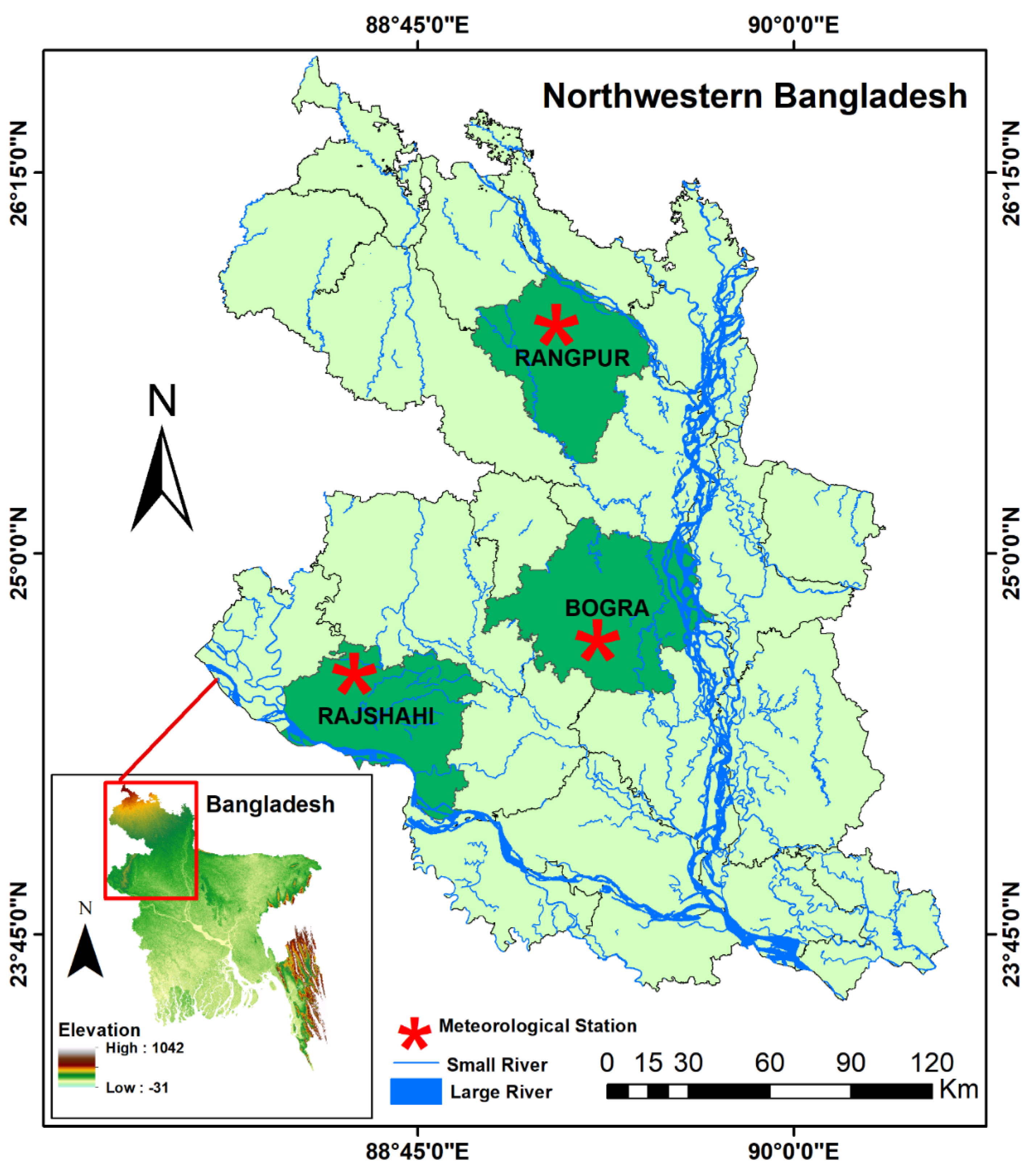
2.1. Case Study Area

The northwestern (NW) hydrological area in Bangladesh’s drought-prone, data-scarce region was chosen as the case study site to assess the accuracy of the aforementioned models ‘predictions. Bangladesh’s northwestern region accounts for 23.5% (34,515 km²) of the country’s overall geographical area. It is subdivided into 16 administrative districts, with Rajshahi, Bogra, and Rangpur selected as case studies for this study (Figure 1). The study area is within 23°47′ N to 25°50′ N latitude and 88°01′ E to 89°48′ E longitude and located on the west of the Brahmaputra River in Bangladesh and north of the Padma River [26]. The population density of the study area is 930 people per square kilometer. Several rivers traverse the region, which Plio-Pleistocene characterizes, and Holocene oxidized red sediments and soils [27]. Figure 1 depicts the northwestern region’s geography and the sites of meteorological stations. The case study region consists of three unique physiographic units: the Barind Tract in the Rajshahi district, the channel–floodplain complexes in the Borga district, and the Himalayan piedmont plain in the Rangpur district [28]. The height of the Barind Tract ranges between 11 and 48 m above mean sea level (AMSL).

In contrast, the channel–floodplain complexes are between 8 and 23 m, and the Himalayan piedmont plain is between 30 and 45 m. The subsurface lithology of the northwest hydrological zone varies considerably. The Barind Tract is primarily a drought-prone water-deficit zone, which often adversely affects agricultural crop output and the inhabitants’ way of life in the studied area [29]. In the district of Bogra, the predominant soil texture is silty loam and clay loam; in Rajshahi, clay loam; and in Rangpur, silty loam.

The northwest area has a dry winter and a humid monsoon season with an unpredictable rainfall pattern. In total, 82% of precipitation occurred between May and October (monsoon season), whereas the remaining 18% occurred between November and April (dry season) [30]. Rajshahi had the lowest average annual rainfall (1428 mm), while Rangpur had the most (2262 mm). Due to the continued effects of climate change, the northwestern region has been experiencing severe occurrences such as flooding and drought, which renders this region more vulnerable to natural disasters [31].

The Rajshahi district receives the least average annual precipitation (1427 mm), while the Rangpur district receives the most (2260 mm). In the Rajshahi district, the monthly mean relative humidity ranges from 62% in March to 87% in July, with a mean of 78%, while in the Rangpur district, the monthly mean relative humidity ranges from 70% in March to 90% in July, with a mean of 65% [32]. In the northwest area, the mean reference evapotranspiration is 1309 mm, which varies spatially and temporally, with the greatest value in Rajshahi and the lowest value in the Rangpur district. Approximately 43% of the reference evapotranspiration occurred during the dry period, whereas 57% occurred during the monsoon season. Rangpur district has a tropical climate that is hot, rainy, and humid [33]. It has a varied monsoon season with a mean annual temperature of 26 °C, ranging from 19 °C in January to 31 °C in August. Numerous monthly variations in meteorological indices indicate that the climate of the Rangpur area is continually evolving [33]. During the summer, some days in the Rajshahi district reach temperatures as high as 45 °C.

In comparison, the temperature decreases up to 5 °C during the winter. The annual mean maximum and lowest temperatures in the Bogra district are 34.6 °C and 11.9 °C, respectively, with a total annual precipitation of 1610 mm. The rate of average temperature increase is projected to be 5.39 °C by the end of the 21st century in the northwestern area, accompanied by a 0.66 mm drop in average precipitation [34]. The elevation of most parts of Bangladesh ranged from 1 to 37.5 m above the mean sea level, which makes for a mainly low-lying “delta-shaped” landform type. Bangladesh, on the other hand, has had trouble obtaining long-term and complete climate datasets, as well as dealing with similar problems caused by nature, such as a complex hydrogeologic and climate system, and by people, such as low economic growth, a lack of good data, and technological issues.

2.2. Data Sources and Quality Control

The Bangladesh Meteorological Department (BMD) operates just 43 meteorological stations around the country, with the majority of them located in the country’s south-eastern regions. BMD only has six meteorological sites in the country’s northwestern area (www.bmd.gov.bd, accessed on 23 December 2022). These six meteorological sites are dispersed irregularly. Because three out of six stations were constructed after 1990, these stations lack the necessary long-term data for determining ETo. When multiple climatic variables were needed, a daily meteorological record from fewer stations was available. Due to these limitations of long-term daily meteorological datasets, only three sites were selected to estimate monthly ETo from 1980 to 2017 for 37 years. These three sites have no data gaps or inconsistencies in the datasets. The three chosen meteorological stations of Rajshahi, Bogra, and Rangpur districts reflect the northwestern United States hydrological area. The recorded daily minimum and maximum temperature (°C), mean relative humidity (%), wind speed (Knots), and sunlight (hours per day⁻¹) values for the three chosen stations were retrieved from the BMD. The BMD has followed World Meteorological Organization rules while collecting and documenting meteorological datasets (WMO) [35].

Before commencing the estimate of the ETo, all datasets were evaluated for quality. Careful quality control of the obtained datasets was undertaken by verifying that all parameters had positive values; for instance, Tmin is less than Tmax, and humidity is less than 100%. The homogeneity tests of the datasets were carried out using the one-way ANOVA test, and the findings indicated that all datasets are significant at a level of 95% (p < 0.05). All datasets were additionally validated by the BMD’s professional and competent quality assurance team.

Table 1. The geographical sites and daily mean values of three selected in situ observational datasets in northwest Bangladesh.

Stations	Latitude (N)	Longitude (E)	Altitude (m)	Tmax (°C)	Tmin (°C)	Rs (MJm−2d−1)	Ra (MJm−2d−1)	U2 (ms−1)	Hr (%)	ETo (mmd−1)
Bogura	24.85	89.37	17.90	29.91	21.04	16.69	32.84	1.06	78.14	3.69
Rajshahi	24.37	88.7	19.50	30.11	20.56	17.25	32.97	1.00	78.18	3.78
Rangpur	25.73	89.27	32.61	28.96	20.25	16.60	32.63	1.03	80.26	3.53

provides a concise geographical and meteorological description of the chosen sites. Meteorological stations cannot directly determine extraterrestrial radiation (Ra), wind speed at the height of 2 m (U2), or global solar radiation (Rs). For instance, the sunshine duration values (n/N) are 0.753 for Bogura, 0.7505 for Rajshahi, and 0.7192 for Rangpur, respectively. The actual height Z of U2 measurements is 18 m for Bogura, 20 m for Rajshahi, and 34 m for Rangpur. We approximated daily Rs, Ra, and U2 using the methods proposed by Allen et al. (1998) and the available meteorological data. Although Allen et al. [36] recommended a = 0.25 and b = 0.5 (or “as” and “bs” as used for this research), these values truly vary with location. The values of these constants in the radiation equation at various locations around the world over the year have already been established in the existing literature. Similar to our study, Adnan et al. [35], Salam and Islam [37], and Salam et al. [38] in Bangladesh, and Dabral et al. [39] in India, applied similar recommended values for their studies. In total, 80% of the dataset was utilized for training, while the remaining 20% was used for testing.

2.3. FAO56 Penman–Monteith Model (FAO56-PM Model)

This research used the FAO56-PM equation to estimate daily ETo. Allen et al. [36] proposed this conventional and widely utilized model. The following Equation (1) states the original statistical form of the FAO56-PM model:

$$\mathrm{ETo}=\frac{0.408\Delta \left({\mathrm{R}}_{\mathrm{n}}- \mathrm{G}\right)+\mathsf{\gamma }\frac{900}{\mathrm{T}+273}{\mathrm{U}}_2\left({\mathrm{e}}_{\mathrm{s}}-{ \mathrm{e}}_{\mathrm{a}}\right)}{\Delta +\mathsf{\gamma }\left(1+0.34{\mathrm{U}}_2\right)}$$

(1)

where, ETo represents the reference evapotranspiration (mmd⁻¹), ${\mathrm{R}}_{\mathrm{n}}$ is the net radiation at the crop surface (MJm⁻² d⁻¹). Allen et al. [38] recommended G (soil heat flux density) =0. FAO’s 56 study describes in full the processes for ETo estimate.

Rn is calculated by Equations (2)–(11):

Rn = Rns − Rnl

(2)

Rns = (1 − α)Rs

(3)

$$\mathrm{Rs}=[\mathrm{as}+\mathrm{bs}\frac{\mathrm{n}}{\mathrm{N}}] \mathrm{Ra}$$

(4)

$$\mathrm{Ra}=\frac{24 \left(60\right)}{\pi } \mathrm{Gsc} \mathrm{dr} \left[\mathsf{\omega }\mathrm{ssin}\right(\mathsf{\varphi }\left)\sin \right(\mathsf{\delta })+\cos (\mathsf{\varphi }\left)\cos \right(\mathsf{\delta }\left)\sin \right(\mathsf{\omega }\mathrm{s}\left)\right]$$

(5)

$$\mathrm{dr}=1 0.033\cos \left(\frac{2\pi }{365}\mathrm{J}\right)$$

(6)

$$\mathsf{\delta }=0.409 \sin \left(\frac{2\pi }{365}\mathrm{J}-1.39\right)$$

(7)

ωs= arccos [−tan (ϕ) tan (δ)]

(8)

Radians = π/180(decimaldegrees)

(9)

$$\mathrm{Rnl}=\mathsf{\sigma }[\frac{{\mathrm{T}}_{\max }{\mathrm{k}}^4+{ \mathrm{T}}_{\min }{\mathrm{K}}^4}{2}](0.34-0.14\surd {\mathrm{e}}_{\mathrm{a}})[1.35\frac{{\mathrm{R}}_{\mathrm{s}}}{{\mathrm{R}}_{\mathrm{so}}}-0.35]$$

(10)

$$\mathrm{Rso}=(0.75+2\times {10}^{-5}\mathrm{Z}) \mathrm{Ra}$$

(11)

U2 is calculated from the following Equation (12), recommended by Allen et al. [36],

$$\mathrm{U}2={\mathrm{U}}_{\mathrm{z}}\frac{4.87}{\mathrm{In}\left(67.8\mathrm{z}-5.42\right)}$$

(12)

where, Rns stands for the net solar or shortwave radiation (MJ m⁻² d⁻¹), Rnl is the net outgoing longwave radiation (MJ m⁻² d⁻¹), Rs is the global solar or shortwave radiation (MJ m⁻² d⁻¹), N and n are, respectively, maximum and actual possible sunshine duration, Ra is extraterrestrial radiation (MJ m⁻² d⁻¹), Gsc is solar constant (0.0820 MJ m⁻² min⁻¹), dr is inverse relative distance Earth–Sun, ωs is the sunset hour angle (rad), ϕ is latitude (rad), δ is the solar declination (rad), J is the number of the day in the year between 1 (1 January) and 365 or 366 (31 December), σ is Stefan–Boltzmann constant (4.903 × 10⁻⁹ MJ K⁻⁴ m⁻² d⁻¹), α is albedo (α = 0.23), Tmaxk and Tmin k are, respectively, maximum and minimum absolute temperatures during 24 h, and Rso is clear sky solar radiation (MJ m⁻² d⁻¹). Allen et al. [36] recommended 0.25 for as and 0.50 for bs. Uz is measured wind speed at Zm above the ground surface (ms⁻²), and z is the respective station elevation above sea level (m).

According to Allen et al. [36], saturation vapor pressure(e_s), actual vapor pressure (e_a), slope vapor pressure curve (∆), and psychrometric constant (γ) are calculated by the following Equations (13)–(19), respectively:

$$e_s=\frac{e^0\left(T_{max}\right)+e^0\left(T_{min}\right)}{2}$$

(13)

$$e^0\left(T_{max}\right)=0.6108 exp\left[\frac{17.27T_{max}}{T_{max}+237.3}\right]$$

(14)

$$e^0\left(T_{min}\right)=0.6108 exp\left[\frac{17.27T_{min}}{T_{min}+237.3}\right]$$

(15)

$$e_a=\frac{Hr\left(mean\right)}{100}\left[\frac{e^0\left(T_{max}\right)+e^0\left(T_{min}\right)}{2}\right]$$

(16)

$$\Delta =\frac{4098\left[0.6108 exp\left(\frac{17.27 T}{T+237.3}\right)\right]}{{\left(T+237.3\right)}^2}$$

(17)

$$\mathsf{\gamma }=\frac{CpP}{\epsilon \lambda }=0.665 \times 10-3\mathrm{P}$$

(18)

$$\mathrm{P}=101.3{\left(\frac{293-0.0065Z}{293}\right)}^{5.26}$$

(19)

where, es represents the mean saturation vapor pressure (kPa), $e^0\left(T_{max}\right) \mathrm{and} e^0\left(T_{min}\right)$ represent the saturation vapor pressure at the maximum and lowest temperatures, Ea represents the actual vapor pressure function (kPa), and Hr represents the mean relative humidity. T_ave, T_max, and T_min are the average, maximum, and minimum air temperatures, respectively, in °C, and exp [ ] is 2.7183 (i.e., the base of natural logarithm) raised to the power [3]. P is atmospheric pressure (kPa), λ is the latent heat of vaporization (2.45 MJ kg⁻¹), Cp is the specific heat at constant pressure (1.013×10⁻³ MJ kg⁻¹ °C⁻¹), ε is s the ratio of water vapor molecular weight to dry molecular air weight (0.622).

3. Methods

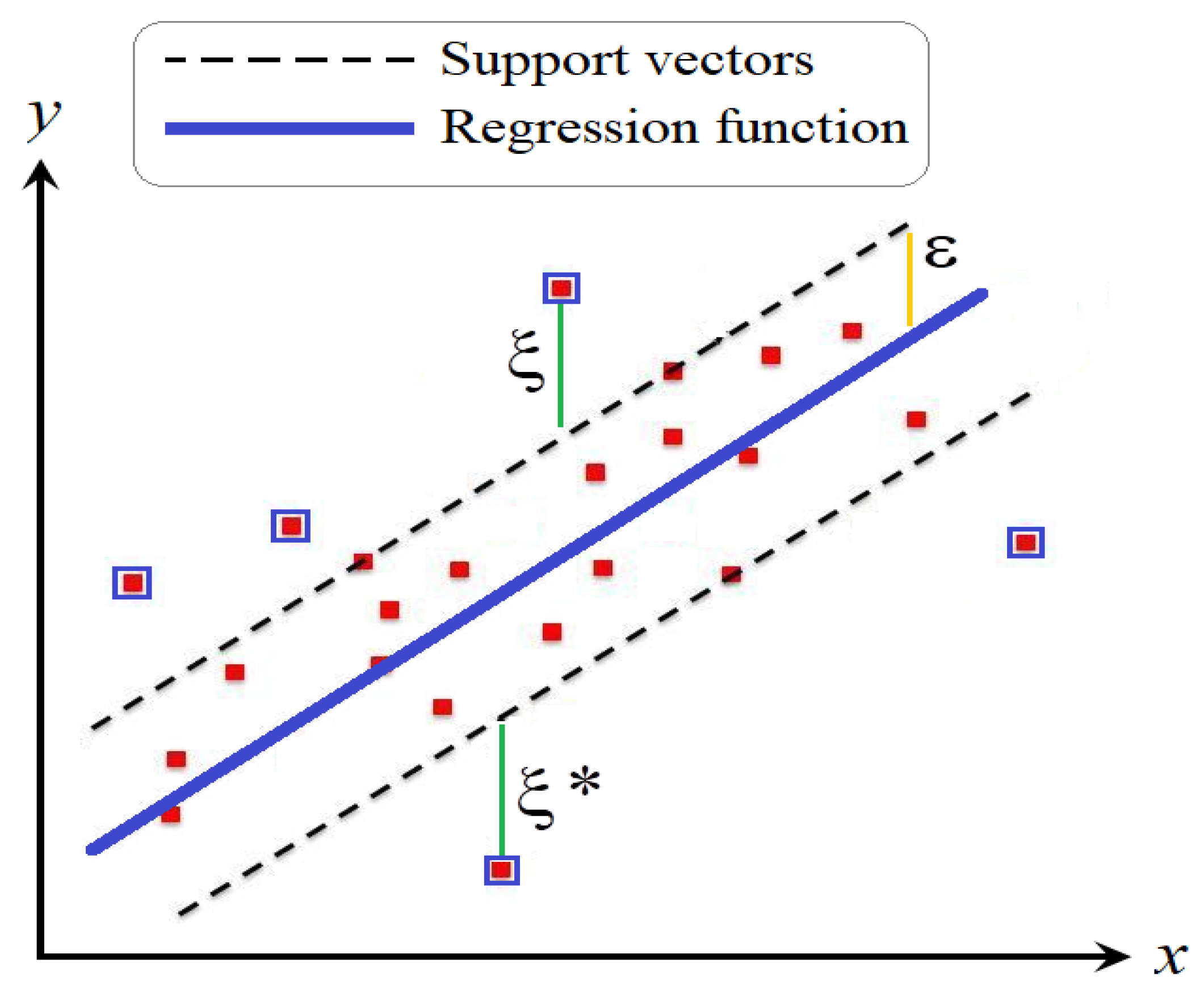
3.1. Machine Learning Model (SVR)

This study employs support vector regression (SVR) as a prevailing and well-known machine learning model to predict ET_o values. It is worth noting that the SVR has already been successfully applied and reported in several hydrological modeling studies [40,41,42].

Consider a training set such as $T=\left\{\left({\mathbf{x}}_{i,}{y}_i\right),i=1,2,\dots ,l\right\}$; the SVR model aims to map the initial data in a higher dimensional feature space. Therefore, the SVR needs to construct a decision function, $f\left(x\right)$, to simulate the nonlinear relationship between the input vector, ${\mathbf{x}}_i$, and the target value, y_i. Assuming M as the order of the polynomial of the hyper-surface, the estimated regression function can be written as below:

$$f\left(x_j\right)=〈\mathbf{w},\mathbf{x}〉+b={\displaystyle \sum _{j=1}^M{\mathrm{w}}_j{\mathrm{x}}_j+b}$$

(20)

where $〈.,.〉$ means the dot product of two parameters and $w_j$ is the coefficient vector. In Figure 2, the geometrical illustration of the linear form of the SVR method is shown. SVR tries to find the widest tube, $\mathsf{\epsilon }-\mathrm{SVR}$, between the support vectors around the hyper-surface, which is the range between $f(x) + \mathsf{\epsilon }$ and $f\left(x\right)-\mathsf{\epsilon }$ ($\mathsf{\epsilon }$ is the permitted error threshold, see Figure 2). Therefore, the objective function, $\raisebox{1ex}{$1$}\!\left/ \!\raisebox{-1ex}{$2$}\right.{‖w‖}^2$, subject to $\left|y_j-f\left(x_j\right)\right|\le \mathsf{\epsilon }$ should be minimized (here y is the target value). For the data outside of the tube, the boundary should be optimized. Thus, two slack factors, $\mathsf{\xi }>0$ and $\mathsf{\xi }*>0$, are introduced and applied for the optimization problem [43].

$$\begin{array}{l}\mathrm{Min}\left(\mathrm{Object} \mathrm{function}=\frac{1}{2}{‖\mathbf{w}‖}^2+C{\displaystyle \sum _{\mathrm{i}=1}^M\mathsf{\xi }+\mathsf{\xi }*}\right)\\ \mathrm{s}.\mathrm{t}. \left\{\begin{array}{l}{y}_j-f\left(x_j\right)\le \epsilon +\mathsf{\xi }*\\ f\left(x_j\right){-y}_j\le \epsilon +\mathsf{\xi }\end{array}\right., \mathrm{j}=1,2,\dots ,\mathrm{M}\end{array}$$

(21)

where the constant C > 0 is the penalty coefficient. It should be noted that in real cases, most data cannot be appropriately separated by a linear hyperplane (hyper-surface).

Thus, kernel functions are used to cope with this problem to map the available data from low-dimensional feature space to a higher response space where a linear separation works properly. In this sense, the radial basis function, RBF, has been used in this study.

$$k\left(x,x_i\right)=exp\left(-\gamma {‖x-x_i‖}^2\right)$$

(22)

where $\gamma$ denotes the kernel’s hyperparameter. In a standard SVR model, tuning parameters (e.g., the values for $C, \epsilon , \mathrm{and} \gamma$) are optimized according to mathematical methodologies such as the least square optimization method. However, based on the conclusion of several researchers [44,45], embedding heuristic algorithms for optimization procedures can improve the accuracy of the standard models. Thus, we have applied integrative SVR models based on individual and hybrid heuristic algorithms. Detailed information regarding the heuristic algorithms and the integration procedure is explained in the following sections.

3.2. Heuristic Optimization Methods (PSO, GWO, and GSA)

In the current research, three types of heuristic algorithms were used either as an individual (e.g., the particle swarm optimization, PSO) or as hybrid algorithms (the grey wolf optimizer, GWO and the gravitational search algorithm, GSA) to optimize the standard SVR model.

The PSO is a well-known population-based optimization algorithm inspired by the social behavior of animals’ behavior for searching food or immigration, such as fish schooling or bird flocking [46]. The PSO method generates the initial population randomly through the search space. During the training process, the best location of each agent (particle) is kept in the algorithm’s memory. Hence, in each iteration, particles in the swarm (the group/herd of the animals) would update their positions based on the following equations [46]:

$$x_{n+1}^i=x_n^i+v_{n+1}^i$$

(23)

$$v_{n+1}^i=\omega v_n^i+c_1{r}_1\left(p_n^i-x_n^i\right)+c_2{r}_2\left(p_n^g-x_n^i\right)$$

(24)

where x and v are the position and velocity vectors, respectively. In addition, i stands for the particle, n is the iteration number in the epoch. $\mathsf{\omega }$ denotes the inertia weight parameter, and r₁ and r₂ represent the two random numbers between zero and unity (rand (0,1)). Pⁱ is the best position achieved by the i^th particle. At the same time, P^g refers to the best position information in the swarm. Similar to the other iteration algorithms, the computation would continue until reaching the final epoch or converging to a predetermined stopping criterion.

Similar to the PSO, the GWO algorithm is another nature-based method inspired by the leadership hierarchy of grey wolf packs as the apex predators. In the GWO, the agents are rated in four types according to the four types of wolves in the leadership hierarchy: alpha, beta, delta, and omega. However, the alpha agents introduce the solution within the searching space. Beta and delta agents represent the second and third-best solutions, and omega agents are the solution candidates. In other words, the training process for seeking the best solution (hunting for the wolves) is carried out by the alpha, beta, and delta wolves. The GWO algorithm generally follows three main steps for searching for the best solution for the response parameter. These steps include [47]:

(i)

Tracking, chasing, and approaching the prey;

(ii)

Pursuing, encircling, and harassing the prey;

(iii)

And finally, getting close to the prey and attacking.

Unlike the previously mentioned PSO and GWO algorithms, the GSA has not considered a nature-based optimization algorithm. However, it is a swarm optimization heuristic algorithm based on Newton’s gravitational law between objects. In this sense, each object with a specific mass exerts a force on the other objects around it. Naturally, the other surrounding objects impose the same force on the object of interest in a mutual way. This process is known as the gravitation force among objects. The gravitational force between two objects complies with two main characteristics: (i) the mass of the objects and (ii) the distance between them [48]. Assuming two objects with a distance equal to R having the masses of M₁ and M₂, the induced gravitational force (F) between them can be calculated as the following equation:

$$F=G\frac{M_1{M}_2}{R^2}$$

(25)

In the above equation, G denotes the gravitational constant.

The GSA aims to find the best solution according to the movement of particles (objects). Having the initial population. The position and velocity of the particles are updated in compliance with the resultant force (F, see Equation (6)) and acceleration (a) associated with each particle along with the G factor. Considering a particle, its velocity and position vectors would be updated in the next iteration as follows:

$$x_{n+1}^i=x_n^i+v_{n+1}^i$$

(26)

$$v_{n+1}^i=r^i{v}_n^i+a_n^i$$

(27)

During the solution process, the particles are attracted and move towards those with greater inertia mass (M). Detailed information regarding the GSA methodology can be found by Rashedi et al. [49].

3.3. Hybrid Optimization Methods (PSOGWO and PSOGSA)

In this study, we have used two hybrid heuristic algorithms, including the PSOGWO (the combination of the particle search swarm optimization, PSO, and the grey wolf optimizer, GWO) and the PSOGSA (the combination of the PSO, and Gravitational Search Algorithm, GSA). In addition to the abovementioned hybrid algorithms, the integrative SVR-PSO model is also applied to evaluate the performances of SVR-PSOGWO and SVR-PSOGSA. In the following, explanations regarding the hybrid optimization methods are given.

-

PSOGWO

Here, the developed hybrid PSOGWO algorithm works on the concepts of the general operation of the original PSO and GWO algorithms (Algorithm 1). It should be noted that the PSO is a robust nature-based algorithm, and it can be successfully utilized for several simulating problems. However, it has been declared that one can reduce the possibility of trapping in local minima by attaching it to the GWO algorithm [50]. In the original PSO algorithm, some particles are allocated random positions that enhance the risk of falling in a local minimum. Attaching the GWO algorithm to the PSO would direct the randomly positioned particles to the improved positions specified by the GWO algorithm. This procedure improves the precision of the PSO algorithm; nonetheless, it encounters the shortcoming of longer running time (computational time). In the following, the pseudo-code for the PSOGWO algorithm is explained. Detailed information regarding the hybridization procedure of the PSOGWO is available at Şenel et al. [50].

Algorithm 1. PSOGWO

•   Setting up parameters   Epoch: the number of iterations (either set by the user or reached according to the other types of stopping criteria)   SP: Initial swarm population number (particles in the PSO algorithm) prob: possibility rate (set by the user) •   Hybrid procedure   Initializing particles in the solution space    FOR i = 1 to Epoch       FOR j = 1 to SP       Run PSO (updating the x and v vectors)       Evaluating the fitness values       Updating Pg (memorizing the best values of the swarm)       IF rand (0,1) < prob then (to avoid trapping in local minima) THEN       Run GWO           Evaluating the fitness of all wolves           Updating the positions of the Alpha, Beta, and delta wolves           Calculating the mean of the position of three best (α, β, δ) wolves           Returning updated values for the particles in the PSO algorithm       END IF    END FOR END FOR

-

PSOGSA

In developing the hybrid version of PSOGSA (Algorithm 1), we tried to cope with the main shortcomings of the individual heuristic algorithms. According to the concepts of forming the GSA, particles move towards the one with greater mass. This procedure makes the algorithm a good candidate for conducting an efficient exploitation phase. Nevertheless, this upside characteristic of the GSA might cause weakness in properly searching the whole response domain, i.e., the deficiency in the global exploring potential. On the other hand, as mentioned earlier, the PSO algorithm has a strong global exploring ability (i.e., exploration phase).

Nevertheless, according to some reports [51], its exploiting phase is not as sufficient as it should be. Therefore, similar to the hybrid PSOGWO algorithm, the hybridization process has been carried out to overcome this drawback using the GSA (instead of the GWO) so that one can evaluate the precision and potential of these two hybrid methods [52]. In the following, the pseudo-code developed for the PSOGSA algorithm is explained. Further information for the applied hybridization procedure of the PSOGSA is available at Song et al. [53].

Algorithm 2. PSOGSA

•   Setting up initial values and parameters     Epoch: the number of iterations; SP: Initial swarm population number; prob: possi bility rate •   Hybrid procedure Initializing particles in the solution space    FOR i = 1 to Epoch       FOR j = 1 to SP       Run PSO       Evaluating the fitness values of the particles updating Pg       IF rand(0,1) < prob then (to avoid trapping in local minima) THEN       Run GSA           Computing the resultant force (F) and the acceleration (a)           Updating values for the velocity and positions (Pi)           Returning updated values for the particles in the PSO algorithm       END IF    END FOR END FOR

3.4. Performance Evaluation

Two novel SVR methods combined with hybrid PSO-GWO and PSO-GSA meta-heuristic algorithms are compared with the single SVR and SVR-PSO method in estimating monthly ET₀ using climatic data involving Tmin, Tmax, Ra, Rs, U2, and HR. The following statistics were utilized for assessing the implemented methods:

$$RMSE:Root Mean Square Error=\sqrt{\frac{1}{N}{\displaystyle \sum }_{i=1}^N{[{(E{T}_0)}_i-{(E{T}_e)}_i]}^2}$$

(28)

$$MAE:Mean Absolute Error=\frac{1}{N}{\displaystyle \sum }_{i=1}^N|{(E{T}_0)}_i-{(E{T}_e)}_i|$$

(29)

$$NSE:Nash-Sutcliffe Efficiency=1-\frac{{{\displaystyle \sum }}_{i=1}^N{[{(E{T}_0)}_i-{(E{T}_e)}_i]}^2}{{{\displaystyle \sum }}_{i=1}^N{[{(E{T}_0)}_i-{\overline{ET}}_0]}^2},-\infty <NSE\le 1$$

(30)

where $E{T}_0, E{T}_e, {\overline{ET}}_0$ are FAO56-PM ET₀, estimated an average FAO56-PM ET₀, respectively, and N indicates the data quantity. Distinct values were attempted to reach the optimal values reported in

Table 2. Parameters setting of each optimization algorithm.

SVR	$C$	10
	$\gamma$	0.1
	$\epsilon$	0.01
	Kernel type	Radial bias function (RBF)
PSO	Cognitive component ($c_1$)	2
	Social component ($c_2$)	2
	Inertia weight	0.2–0.9
GWO	$a$	decreased from 2 to 0
GSA	Initial gravitational constant $\left(G_0\right)$	100
	Search parameter $\left(\alpha \right)$	20
PSOGWO	As in both PSO and GWO
PSOGSA	As in both PSO and GSA
All algorithms	Population	25
	Number of iterations	100
	Number of runs for each algorithm	8

. This table also represents each algorithm’s population number, iterations, and several runs.

Table 3. The input combinations used for model development.

Input Combinations	Variables
(i)	Tmin, Tmax
(ii)	Tmin, Tmax, Ra
(iii)	Tmin, Tmax, Rs
(iv)	Tmin, Tmax, U2
(v)	Tmin, Tmax, Ra, Rs
(vi)	Tmin, Tmax, Rs, U2
(vii)	Tmin, Tmax, Ra, U2
(viii)	Tmin, Tmax, Ra, Rs, U2
(ix)	Tmin, Tmax, Ra, Rs, U2, HR

lists the input combinations considered in this study and the corresponding variables.

4. Results and Discussion

Four AI models with nine different input combinations (Table 3) are applied to three selected climatic stations.

Table 4. The results of Station 1 (Bogra) using SVR-based models.

Models	Input Combinations	Training				Testing
		RMSE	MAE	NSE	R2	RMSE	MAE	NSE	R2
SVR	I	0.508	0.403	0.682	0.682	0.597	0.511	0.584	0.692
	II	0.396	0.310	0.807	0.807	0.390	0.324	0.823	0.834
	III	0.209	0.154	0.946	0.946	0.432	0.316	0.782	0.875
	IV	0.395	0.307	0.808	0.821	0.470	0.332	0.743	0.749
	V	0.190	0.136	0.955	0.955	0.326	0.198	0.876	0.898
	VI	0.172	0.128	0.963	0.963	0.441	0.306	0.773	0.866
	VII	0.311	0.240	0.881	0.881	0.379	0.269	0.833	0.863
	VIII	0.147	0.107	0.974	0.974	0.373	0.250	0.838	0.891
	IX	0.100	0.073	0.988	0.988	0.352	0.232	0.856	0.912
SVR-PSO	I	0.411	0.338	0.792	0.803	0.498	0.419	0.710	0.743
	II	0.308	0.232	0.883	0.884	0.364	0.305	0.845	0.871
	III	0.182	0.133	0.959	0.960	0.398	0.290	0.815	0.888
	IV	0.317	0.240	0.877	0.877	0.430	0.312	0.784	0.792
	V	0.153	0.109	0.971	0.971	0.353	0.244	0.855	0.909
	VI	0.152	0.112	0.972	0.972	0.426	0.296	0.788	0.876
	VII	0.241	0.190	0.929	0.929	0.346	0.263	0.860	0.883
	VIII	0.127	0.096	0.980	0.980	0.420	0.318	0.794	0.905
	IX	0.097	0.071	0.988	0.989	0.335	0.222	0.869	0.923
SVR- PSOGSA	I	0.369	0.293	0.832	0.833	0.490	0.391	0.720	0.761
	II	0.238	0.183	0.930	0.930	0.368	0.291	0.842	0.916
	III	0.131	0.098	0.979	0.979	0.309	0.213	0.888	0.901
	IV	0.281	0.221	0.903	0.903	0.420	0.305	0.794	0.805
	V	0.127	0.093	0.980	0.980	0.283	0.181	0.907	0.919
	VI	0.118	0.083	0.983	0.983	0.472	0.367	0.740	0.890
	VII	0.215	0.170	0.943	0.943	0.304	0.216	0.892	0.893
	VIII	0.109	0.076	0.985	0.985	0.369	0.247	0.841	0.897
	IX	0.061	0.043	0.995	0.995	0.292	0.178	0.900	0.927
SVR- PSOGWO	I	0.316	0.247	0.877	0.877	0.512	0.388	0.694	0.782
	II	0.233	0.177	0.933	0.933	0.298	0.241	0.897	0.931
	III	0.148	0.109	0.973	0.973	0.330	0.219	0.873	0.898
	IV	0.283	0.222	0.902	0.902	0.390	0.278	0.823	0.832
	V	0.106	0.078	0.986	0.986	0.306	0.208	0.891	0.927
	VI	0.122	0.086	0.982	0.982	0.446	0.343	0.768	0.892
	VII	0.215	0.168	0.943	0.943	0.305	0.233	0.892	0.922
	VIII	0.113	0.082	0.984	0.984	0.301	0.212	0.894	0.929
	IX	0.061	0.042	0.995	0.995	0.277	0.167	0.911	0.933

sums up the training and testing results of the implemented methods in estimating the ETo of Bogra Station. In all methods, full data offer the highest accuracy, and the SVR-PSOGWO acts better than the other models; improvement in RMSE is 27%, 21%, and 5% in the testing stage compared to SVR, SVR-PSO, and SVR-PSOGSA, respectively. Other models are ranked from best to worst as SVR-PSOGSA > SVR-PSO > SVR in the estimation of monthly ETo.

Training efficiencies of the SVR-PSOGWO and SVR-GSA are almost equal, and they could approximate the phenomenon better compared to SVR and SVR-PSO; viz. NSE increases from 0.988 to 0.995, and RMSE decreases from 0.073/0.071 to 0.042/0.043. Another important information derived from the results is that the second input case, including Tmin, Tmax, and Ra, also offers good accuracy in estimating monthly ETo for this station. This might carry importance in practical applications because measuring temperatures is very easy, and Ra can be directly calculated from the Julian date.

Table 5. The results of Station 2 (Rajshahi) using SVR-based models.

Models	Input Combinations	Training				Testing
		RMSE	MAE	NSE	R2	RMSE	MAE	NSE	R2
SVR	I	0.345	0.266	0.892	0.892	0.550	0.414	0.717	0.856
	II	0.307	0.231	0.914	0.914	0.454	0.320	0.807	0.883
	III	0.250	0.176	0.943	0.943	0.358	0.286	0.880	0.908
	IV	0.281	0.225	0.928	0.928	0.395	0.315	0.854	0.873
	V	0.213	0.144	0.959	0.959	0.319	0.226	0.909	0.919
	VI	0.324	0.258	0.905	0.905	0.454	0.363	0.807	0.843
	VII	0.293	0.236	0.922	0.922	0.393	0.318	0.855	0.864
	VIII	0.261	0.201	0.938	0.947	0.366	0.277	0.875	0.903
	IX	0.323	0.228	0.905	0.921	0.327	0.239	0.906	0.913
SVR-PSO	I	0.306	0.231	0.915	0.915	0.527	0.400	0.740	0.872
	II	0.260	0.191	0.939	0.939	0.431	0.336	0.826	0.906
	III	0.226	0.151	0.954	0.955	0.346	0.271	0.888	0.918
	IV	0.254	0.199	0.941	0.942	0.392	0.293	0.857	0.881
	V	0.208	0.143	0.961	0.961	0.290	0.226	0.921	0.936
	VI	0.182	0.138	0.970	0.970	0.315	0.246	0.907	0.920
	VII	0.266	0.209	0.936	0.936	0.345	0.261	0.889	0.911
	VIII	0.206	0.152	0.961	0.962	0.315	0.247	0.907	0.922
	IX	0.227	0.173	0.953	0.953	0.298	0.230	0.917	0.929
SVR- PSOGSA	I	0.276	0.206	0.931	0.931	0.525	0.412	0.742	0.875
	II	0.245	0.182	0.946	0.946	0.379	0.305	0.865	0.928
	III	0.186	0.121	0.969	0.969	0.302	0.210	0.915	0.932
	IV	0.223	0.175	0.955	0.955	0.377	0.279	0.867	0.893
	V	0.192	0.121	0.967	0.967	0.271	0.199	0.931	0.945
	VI	0.153	0.111	0.979	0.979	0.302	0.219	0.915	0.928
	VII	0.218	0.166	0.957	0.957	0.316	0.235	0.907	0.920
	VIII	0.134	0.096	0.984	0.984	0.241	0.144	0.946	0.947
	IX	0.092	0.052	0.992	0.992	0.252	0.147	0.941	0.944
SVR- PSOGWO	I	0.264	0.197	0.937	0.937	0.496	0.385	0.770	0.884
	II	0.243	0.177	0.946	0.946	0.389	0.316	0.859	0.939
	III	0.194	0.127	0.966	0.966	0.312	0.233	0.909	0.931
	IV	0.199	0.152	0.964	0.964	0.317	0.249	0.906	0.916
	V	0.180	0.112	0.971	0.971	0.255	0.188	0.939	0.943
	VI	0.130	0.088	0.985	0.985	0.274	0.184	0.930	0.936
	VII	0.199	0.148	0.964	0.964	0.298	0.228	0.917	0.933
	VIII	0.111	0.071	0.989	0.989	0.270	0.191	0.932	0.936
	IX	0.082	0.047	0.994	0.994	0.248	0.145	0.943	0.950

lists the accuracy of the single and hybrid SVR-based models for various input cases of Rajshahi Station. In contrast to the previous station, the methods produced the best accuracy in different input cases. The SVR-PSOGSA with Tmin, Tmax, Ra, Rs, and U2 acted better than the other models; improvements in RMSE by 32%, 20%, and 3% in the testing stage compared to the SVR, SVR-PSO, and SVR-PSOGWO, respectively. The SVR-PSOGWO, SVR-PSO, and SVR follow the best accuracy of SVR-PSOGSA in estimating monthly ETo. In the training (simulation) stage, however, the SVR-PSOGWO is better fitted to data than SVR-PSOGSA. In this station, the second input case (Tmin, Tmax, Ra) may also be another alternative in estimating monthly ETo when the other climatic data (Rs, U2, and HR) are missing. The other important thing is a slight difference between the input cases V and IX for the SVR-PSOGWO. This input case (Tmin, Tmax, Ra, Rs) also offers good accuracy in all methods. In this station, Rs seems more effective on ETo than Bogra Station, which can be seen from the differences between II and V input cases.

The SVR-based methods’ training and testing results are summarized in

Table 6. The results of Station 3 (Rangpur) using SVR-based models.

Models	Input Combinations	Training				Testing
		RMSE	MAE	NSE	R2	RMSE	MAE	NSE	R2
SVR	I	0.369	0.276	0.831	0.831	0.516	0.412	0.651	0.773
	II	0.281	0.180	0.902	0.902	0.390	0.316	0.800	0.887
	III	0.240	0.169	0.929	0.929	0.352	0.230	0.838	0.878
	IV	0.348	0.254	0.850	0.850	0.446	0.331	0.739	0.787
	V	0.205	0.133	0.948	0.948	0.392	0.264	0.798	0.879
	VI	0.206	0.149	0.948	0.948	0.339	0.222	0.850	0.882
	VII	0.297	0.193	0.890	0.890	0.323	0.251	0.863	0.876
	VIII	0.171	0.111	0.964	0.964	0.306	0.179	0.877	0.890
	IX	0.139	0.086	0.976	0.976	0.246	0.143	0.920	0.923
SVR-PSO	I	0.345	0.256	0.852	0.853	0.518	0.413	0.649	0.773
	II	0.250	0.195	0.922	0.924	0.383	0.306	0.808	0.885
	III	0.228	0.159	0.936	0.938	0.320	0.231	0.866	0.896
	IV	0.286	0.234	0.898	0.905	0.416	0.325	0.773	0.793
	V	0.152	0.109	0.971	0.971	0.317	0.211	0.868	0.899
	VI	0.167	0.113	0.966	0.966	0.323	0.217	0.863	0.884
	VII	0.234	0.166	0.932	0.932	0.318	0.245	0.868	0.891
	VIII	0.135	0.100	0.977	0.977	0.299	0.184	0.883	0.909
	IX	0.099	0.064	0.988	0.988	0.228	0.145	0.932	0.936
SVR- PSOGSA	I	0.253	0.198	0.921	0.921	0.490	0.383	0.685	0.793
	II	0.235	0.183	0.932	0.932	0.389	0.316	0.802	0.888
	III	0.163	0.120	0.967	0.967	0.290	0.209	0.889	0.909
	IV	0.255	0.198	0.919	0.919	0.397	0.309	0.793	0.804
	V	0.089	0.062	0.990	0.990	0.238	0.169	0.926	0.945
	VI	0.106	0.078	0.986	0.986	0.296	0.192	0.885	0.904
	VII	0.149	0.109	0.973	0.973	0.323	0.251	0.863	0.895
	VIII	0.122	0.084	0.981	0.981	0.262	0.188	0.910	0.942
	IX	0.098	0.072	0.988	0.988	0.242	0.177	0.923	0.943
SVR- PSOGWO	I	0.234	0.178	0.932	0.932	0.524	0.407	0.640	0.795
	II	0.179	0.138	0.960	0.960	0.385	0.314	0.805	0.890
	III	0.150	0.109	0.972	0.972	0.294	0.210	0.886	0.918
	IV	0.204	0.157	0.948	0.948	0.391	0.295	0.800	0.825
	V	0.086	0.059	0.991	0.991	0.243	0.184	0.922	0.939
	VI	0.100	0.071	0.988	0.988	0.342	0.237	0.847	0.898
	VII	0.172	0.128	0.963	0.963	0.325	0.247	0.861	0.905
	VIII	0.106	0.070	0.986	0.986	0.278	0.203	0.899	0.939
	IX	0.041	0.029	0.998	0.998	0.200	0.132	0.948	0.951

for Rangpur Station. The SVR, SVR-PSO, and SVR-PSOGWO offered the best accuracy for the IX input case, while the SVR-PSOGSA had the best outcomes for V inputs. However, there is a slight difference between inputs IX and V for this method. The SVR-PSOGWO with the Tmin, Tmax, Ra, Rs, U2, and HR acted better than the other models; improvements in RMSE by 23%, 14%, and 19% in the testing stage compared to SVR, SVR-PSO, and SVR-PSOGSA, respectively. The other models are ranked as SVR-PSOGSA > SVR-PSO > SVR in the estimation of monthly ETo. However, variations in the predictive capabilities between two novel MA models using the combinations of three input climatic variables plans (Tmax, Tmin, and Ra) were slight (RMSE < 10%). As evident from the first part of (columns 3–6) Table 6, the training (simulation) accuracy of the SVR-PSOGWO is also better than the other models; NSE increases from 0.976/0.988/0.990 to 0.998, and RMSE decreases from 0.139/0.099/0.089 to 0.041 by applying the SVR-PSOGWO compared to SVR/SVR-PSO/SVR-PSOGSA.

Table 4, Table 5 and Table 6 clearly show that the SVR-PSOGWO generally offered better accuracy than the other methods in estimating monthly ETo. In the second station, the SVR-PSOGSA performed superior to the SVR-PSOGWO, but the difference was marginal. In addition, the SVR-PSOGSA produced inferior results compared to SVR-PSO in the third station. It is also clear that the single SVR offered the worst outcomes in all stations. This matter indicates the necessity of hybrid metaheuristic algorithms in the training of the SVR method in ETo prediction. The input combination of Tmin, Tmax, and Rs (V input case) also offered good accuracy in ETo estimation.

Figure 3, Figure 4 and Figure 5 reveal the time variation diagrams of the FAO56-PM ETo and estimated ETo by the optimal SVR-based models for the Bogra, Rajshahi, and Rangpur stations, respectively. It is clear from the figures that the estimates of the SVR-based hybrid models are closer to the FAO56-PM ETo values than the single SVR model.

The scatter diagrams of the estimated ETo are illustrated in Figures S1–S3 (see Supplementary Materials) for the three stations. All graphs clearly show that the SVR-PSOGWO has less scattered estimates with the highest R2 values (0.9334, 0.9508, 0.9501) for the Bogra, Rajshahi, and Rangpur stations, respectively. At the same time, the single SVR provides the most scattered estimations.

Similar to our study, Granata [54] found that the SVR was the weakest model in the humid tropical region of Florida, USA. Shiri [55] stated that hybrid tree-based methods were effectively used for monthly ETo forecasting in southern Iran. Similarly, Huang et al. [56] argued that SVM models showed the worst performance with the lowest increases in testing RMSE from 4.1% to 37.3%. Moreover, the metaheuristic algorithms, e.g., SVR-PSOGWO and SVR-PSOGSA models, generally perform better for classification issues but lower for regression issues because they cannot give static outputs. In such a case, these two novel MA tools cannot produce better prediction precision, which leads to an overfitting issue when noisy testing data are employed for estimating ET_o. Overall, the SVR-PSOGWO and SVR-PSOGSA offer better accuracy than the SVR-PSO method in monthly ETo estimation. The main advantages of these hybrid algorithms (GWO and GSA) are incorporated to improve the exploitation ability of PSO, as PSO is known for better exploration but lags in exploitation. However, the two novels’ MA models showed stability with a satisfactory % increase with the lowest increases in the testing RMSE stage.

Salam and Islam [37] found similar results in Bangladesh’s subhumid tropical region. On the other hand, the SVR and SVR-PSO models have many hyper-variables, which need to be carefully tuned for monthly ETo purposes. Our findings suggest that the two newly novel metaheuristic algorithm, with much development upon the traditional SVR model, are a promising tool for preventing the difficulty of the overfitting issue. Thus, K-fold cross-validation is needed to select the optimal parameter and validate the better stability of the soft computing methods. These deserve further investigation.

Khosravi et al. [57] investigated the accuracy of four ANFIS including single ANFIS, hybrid ANFIS models tuned with differential evolution (ANFIS-DE), genetic algorithm (ANFIS-GA), and imperialistic competitive algorithm (ANFIS-ICA), and five data mining models including M5P, random forest (RF), random tree (RT), reduced error runing tree and Kstar models in predicting monthly ETo of Baghdad and Mosul (Iraq) using different meteorological input combinations involving sunshine hours (n), maximum and minimum temperature (Tmax and Tmin), wind speed (U2), rainfall (P), and relative humidity (HR). For the Bagdat Station, all the above-mentioned models except RT provided the best accuracy for the input combination of n, Tmax, and RH, while for the Mosul station, the input combinations of (Tmax, Tmin, n, HR, and U2) and (Tmax, Tmin, n, HR, U2, P) produced best ETo predictions. Khosravi et al. [57,58] reported that the best model accuracy varies concerning the type of the machine learning or data mining methods. This can be explained by the fact that each method has a different structure and different calculation processes.

Reasonably, many soft computing methods generally consider a sole dataset for validating for testing, which may mislead or give partly strong conclusions because the performance capabilities are solely described to an exact distribution of the main dataset and may not be identical [16,30]. The definition of the data combination included in each data combination is important for evaluating the method’s performance. Therefore, the performance of any machine learning method is favorably based on the data distributions and climatic areas. For example, an analogous model showed various performances in various cited works under different climate conditions [59]. Similar to this study, some scholars, e.g., Adnan et al. [60], reported that the hybrid model outperformed other state-of-the-art models. Thus, our work suggests that the SVR-based metaheuristic algorithm can be a likely soft computing method for good accuracy and consistency for monthly ETo prediction using limited datasets in the data-scarce humid region of north-western Bangladesh and is applicable for like climatic settings around the world. However, further study is needed to assess the performance of potential SVR-based metaheuristic models at different time durations, including hourly or daily basis or in other analogous areas, worldwide with humid tropical climate conditions

5. Conclusions

The present study investigated the ability of two novel SVR methods merged with hybrid PSOGSA and PSOGWO meta-heuristic algorithms in estimating ETo using climatic data as inputs. Having a better evaluation, the SVR-PSOGSA and SVR-PSOGWO methods were also compared with single SVR and SVR-PSO methods. The outcomes provided the following conclusions:

(i)

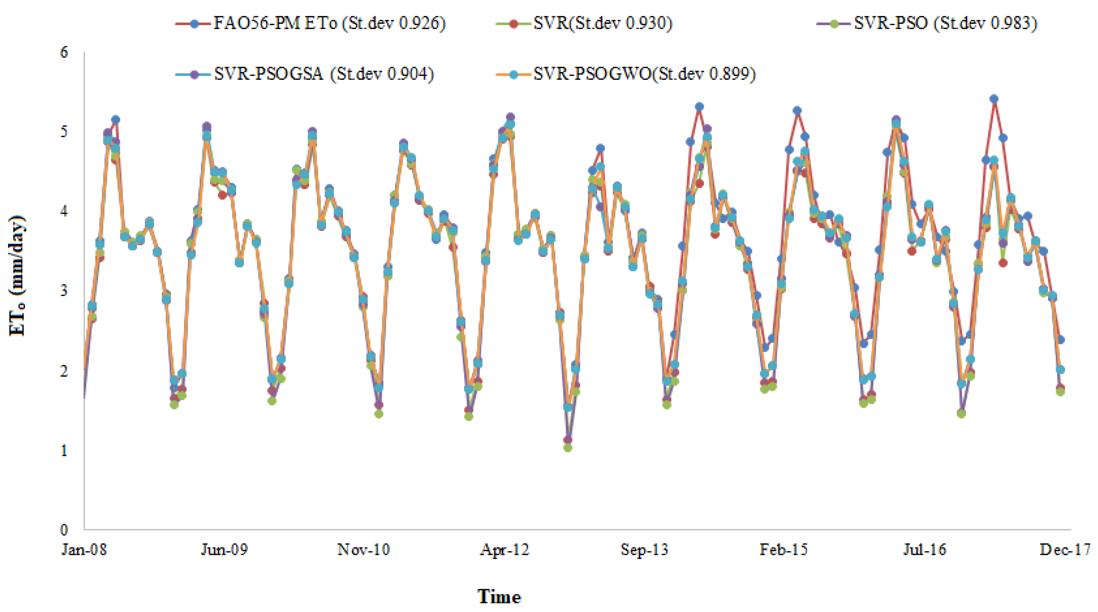
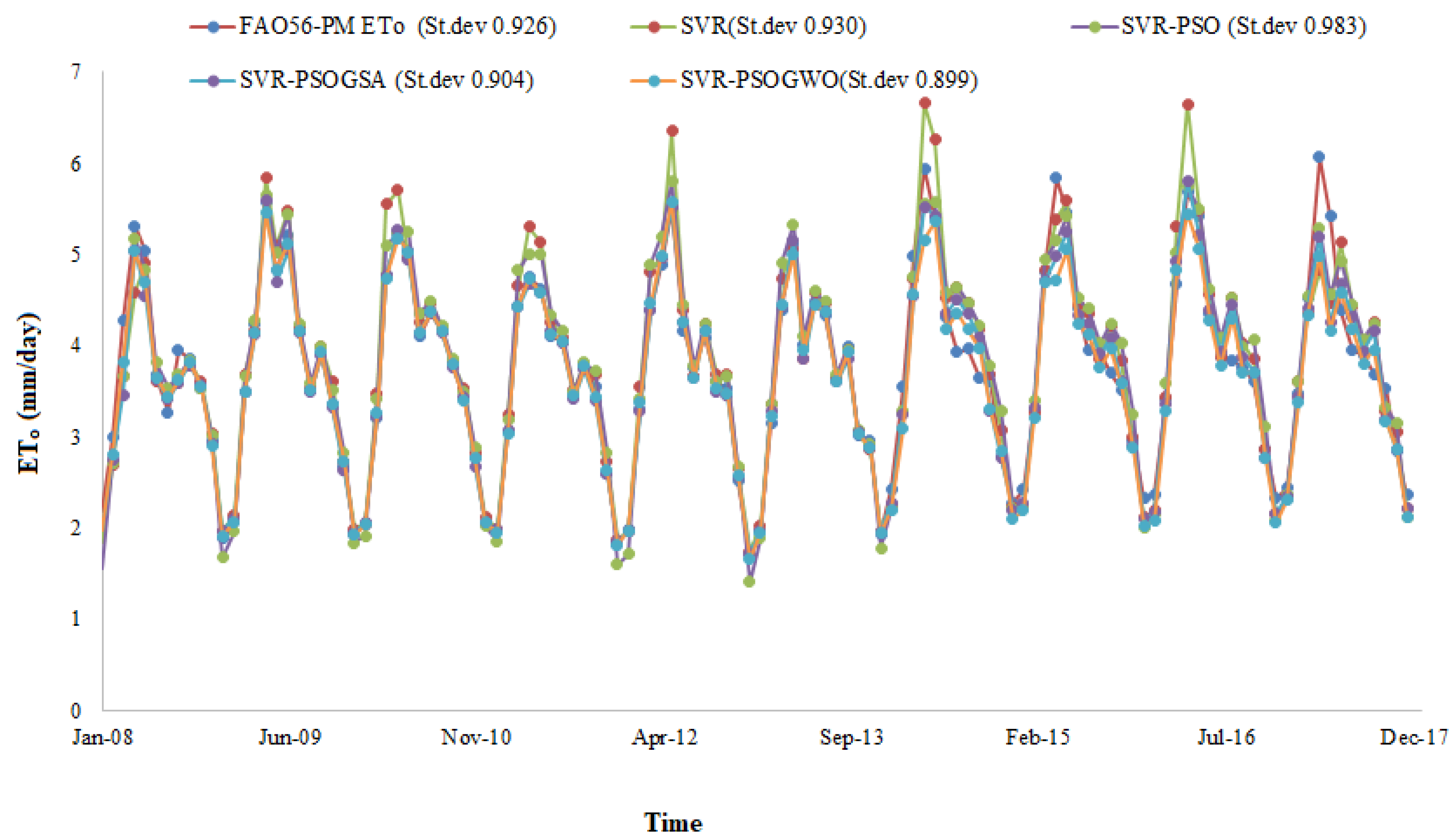
Monthly discharge, Tmin, Tmax, Ra, Rs, U2, and HR data from three stations were used for assessing the above-mentioned methods. Based on the root mean square error, mean absolute error, Nash–Sutcliffe efficiency and determination coefficient and graphical methods, the SVR–PSOGWO was superior to the other methods, followed by the SVR–PSOGSA, SVR–PSO, and SVR. This implies the necessity of hybrid metaheuristic algorithms in SVR training.

(ii)

It was observed that the input combination involving whole climatic data generally produced the best accuracy. The SVR–PSOGWO with Tmin, Tmax, Ra, Rs, and U2 inputs improved the accuracy of single SVR by 27%, 32%, and 23% for Bogra, Rajshahi, and Rangpur stations with respect to root mean square errors in the testing stage, respectively. The second input combination comprising Tmin, Tmax, and Ra also provided good accuracy (NSE ranges from 0.808 to 0.897). The models with this input combination can be a good alternative when other climatic data are unavailable. The viability of the presented hybrid metaheuristic algorithms can be assessed for improving other machine learning methods such as extreme leaning machine, neural networks, or neuro-fuzzy systems in future studies.

References

1. Bozkurt Çolak, Y.; Yazar, A.; Alghory, A.; Tekin, S. Evaluation of crop water stress index and leaf water potential for differentially irrigated quinoa with surface and subsurface drip systems. Irrig. Sci. 2021, 39, 81–100. [Google Scholar] [CrossRef]
2. Huang, D.; Wang, J.; Khayatnezhad, M. Estimation of Actual Evapotranspiration Using Soil Moisture Balance and Remote Sensing. Iran. J. Sci. Technol. Trans. Civ. Eng. 2021, 45, 2779–2786. [Google Scholar] [CrossRef]
3. Ghiat, I.; Mackey, H.R.; Al-Ansari, T. A Review of Evapotranspiration Measurement Models, Techniques and Methods for Open and Closed Agricultural Field Applications. Water 2021, 13, 2523. [Google Scholar] [CrossRef]
4. Lugato, E.; Lavallee, J.M.; Haddix, M.L.; Panagos, P.; Cotrufo, M.F. Different climate sensitivity of particulate and mineral-associated soil organic matter. Nat. Geosci. 2021, 14, 295–300. [Google Scholar] [CrossRef]
5. Shah, S.; Duan, Z.; Song, X.; Li, R.; Mao, H.; Liu, J.; Ma, T.; Wang, M. Evaluating the added value of multi-variable calibration of SWAT with remotely sensed evapotranspiration data for improving hydrological modeling. J. Hydrol. 2021, 603, 127046. [Google Scholar] [CrossRef]
6. Fan, G.; Sarabandi, A.; Yaghoobzadeh, M. Evaluating the climate change effects on temperature, precipitation and evapotranspiration in eastern Iran using CMPI5. Water Supply 2021, 21, 4316–4327. [Google Scholar] [CrossRef]
7. Machakaire, A.T.B.; Steyn, J.M.; Franke, A.C. Assessing evapotranspiration and crop coefficients of potato in a semi-arid climate using Eddy Covariance techniques. Agric. Water Manag. 2021, 255, 107029. [Google Scholar] [CrossRef]
8. Makwana, J.J.; Tiwari, M.K.; Deora, B.S. Development and comparison of artificial intelligence models for estimating daily reference evapotranspiration from limited input variables. Smart Agric. Technol. 2023, 3, 100115. [Google Scholar] [CrossRef]
9. Rodrigues, G.C.; Braga, R.P. Estimation of Reference Evapotranspiration during the Irrigation Season Using Nine Temperature-Based Methods in a Hot-Summer Mediterranean Climate. Agriculture 2021, 11, 124. [Google Scholar] [CrossRef]
10. Samadi, S.Z. Assessing the sensitivity of SWAT physical parameters to potential evapotranspiration estimation methods over a coastal plain watershed in the southeastern United States. Hydrol. Res. 2016, 48, 395–415. [Google Scholar] [CrossRef]
11. Gisolo, D.; Previati, M.; Bevilacqua, I.; Canone, D.; Boetti, M.; Dematteis, N.; Balocco, J.; Ferrari, S.; Gentile, A.; N’Sassila, M.; et al. A calibration free radiation driven model for estimating actual evapotranspiration of mountain grasslands (CLIME-MG). J. Hydrol. 2022, 610, 127948. [Google Scholar] [CrossRef]
12. Abeysiriwardana, H.D.; Muttil, N.; Rathnayake, U. A Comparative Study of Potential Evapotranspiration Estimation by Three Methods with FAO Penman–Monteith Method across Sri Lanka. Hydrology 2022, 9, 206. [Google Scholar] [CrossRef]
13. Wanniarachchi, S.; Sarukkalige, R. A Review on Evapotranspiration Estimation in Agricultural Water Management: Past, Present, and Future. Hydrology 2022, 9, 123. [Google Scholar] [CrossRef]
14. Tejada, A.T.; Ella, V.B.; Lampayan, R.M.; Reaño, C.E. Modeling Reference Crop Evapotranspiration Using Support Vector Machine (SVM) and Extreme Learning Machine (ELM) in Region IV-A, Philippines. Water 2022, 14, 754. [Google Scholar] [CrossRef]
15. Abedi-Koupai, J.; Dorafshan, M.-M.; Javadi, A.; Ostad-Ali-Askari, K. Estimating potential reference evapotranspiration using time series models (case study: Synoptic station of Tabriz in northwestern Iran). Appl. Water Sci. 2022, 12, 212. [Google Scholar] [CrossRef]
16. Chia, M.Y.; Huang, Y.F.; Koo, C.H. Improving reference evapotranspiration estimation using novel inter-model ensemble approaches. Comput. Electron. Agric. 2021, 187, 106227. [Google Scholar] [CrossRef]
17. Dou, X.; Yang, Y. Evapotranspiration estimation using four different machine learning approaches in different terrestrial ecosystems. Comput. Electron. Agric. 2018, 148, 95–106. [Google Scholar] [CrossRef]
18. Nourani, V.; Elkiran, G.; Abdullahi, J. Multi-station artificial intelligence based ensemble modeling of reference evapotranspiration using pan evaporation measurements. J. Hydrol. 2019, 577, 123958. [Google Scholar] [CrossRef]
19. Antonopoulos, V.Z.; Antonopoulos, A.V. Daily reference evapotranspiration estimates by artificial neural networks technique and empirical equations using limited input climate variables. Comput. Electron. Agric. 2017, 132, 86–96. [Google Scholar] [CrossRef]
20. Zhang, G.; Liu, B.; Zhu, T.; Zhou, A.; Zhou, W. Visual privacy attacks and defenses in deep learning: A survey. Artif. Intell. Rev. 2022, 55, 4347–4401. [Google Scholar] [CrossRef]
21. Emadi, A.; Zamanzad-Ghavidel, S.; Fazeli, S.; Zarei, S.; Rashid-Niaghi, A. Multivariate modeling of pan evaporation in monthly temporal resolution using a hybrid evolutionary data-driven method (case study: Urmia Lake and Gavkhouni basins). Environ. Monit. Assess. 2021, 193, 355. [Google Scholar] [CrossRef] [PubMed]
22. Mehdizadeh, S. Estimation of daily reference evapotranspiration (ETo) using artificial intelligence methods: Offering a new approach for lagged ETo data-based modeling. J. Hydrol. 2018, 559, 794–812. [Google Scholar] [CrossRef]
23. Tikhamarine, Y.; Malik, A.; Souag-Gamane, D.; Kisi, O. Artificial intelligence models versus empirical equations for modeling monthly reference evapotranspiration. Environ. Sci. Pollut. Res. 2020, 27, 30001–30019. [Google Scholar] [CrossRef] [PubMed]
24. Tikhamarine, Y.; Malik, A.; Kumar, A.; Souag-Gamane, D.; Kisi, O. Estimation of monthly reference evapotranspiration using novel hybrid machine learning approaches. Hydrol. Sci. J. 2019, 64, 1824–1842. [Google Scholar] [CrossRef]
25. Seifi, A.; Riahi, H. Estimating daily reference evapotranspiration using hybrid gamma test-least square support vector machine, gamma test-ANN, and gamma test-ANFIS models in an arid area of Iran. J. Water Clim. Chang. 2018, 11, 217–240. [Google Scholar] [CrossRef]
26. Hossain, M.A.; Rahman, M.M.; Hasan, S.S. Application of combined drought index to assess meteorological drought in the south western region of Bangladesh. Phys. Chem. Earth Parts A/B/C 2020, 120, 102946. [Google Scholar] [CrossRef]
27. Mojid, M.A.; Aktar, S.; Mainuddin, M. Rainfall-induced recharge-dynamics of heavily exploited aquifers—A case study in the North-West region of Bangladesh. Groundw. Sustain. Dev. 2021, 15, 100665. [Google Scholar] [CrossRef]
28. Sumon, K.A.; Rashid, H.; Peeters, E.T.H.M.; Bosma, R.H.; Van den Brink, P.J. Environmental monitoring and risk assessment of organophosphate pesticides in aquatic ecosystems of north-west Bangladesh. Chemosphere 2018, 206, 92–100. [Google Scholar] [CrossRef]
29. Jamal, M.R.; Kristiansen, P.; Kabir, M.J.; Kumar, L.; Lobry de Bruyn, L. Trajectories of cropping system intensification under changing environment in south-west coastal Bangladesh. Int. J. Agric. Sustain. 2022, 20, 722–742. [Google Scholar] [CrossRef]
30. Dewan, A.; Shahid, S.; Bhuian, M.H.; Hossain, S.M.J.; Nashwan, M.S.; Chung, E.-S.; Hassan, Q.K.; Asaduzzaman, M. Developing a high-resolution gridded rainfall product for Bangladesh during 1901–2018. Sci. Data 2022, 9, 471. [Google Scholar] [CrossRef]
31. Salehie, O.; Ismail, T.; Shahid, S.; Ahmed, K.; Adarsh, S.; Asaduzzaman, M.; Dewan, A. Ranking of gridded precipitation datasets by merging compromise programming and global performance index: A case study of the Amu Darya basin. Theor. Appl. Climatol. 2021, 144, 985–999. [Google Scholar] [CrossRef]
32. Pour, S.H.; Shahid, S.; Chung, E.-S.; Wang, X.-J. Model output statistics downscaling using support vector machine for the projection of spatial and temporal changes in rainfall of Bangladesh. Atmos. Res. 2018, 213, 149–162. [Google Scholar] [CrossRef]
33. Wahiduzzaman, M.; Luo, J.-J. A statistical analysis on the contribution of El Niño–Southern Oscillation to the rainfall and temperature over Bangladesh. Meteorol. Atmos. Phys. 2021, 133, 55–68. [Google Scholar] [CrossRef]
34. Rouf, M.A.; Uddin, M.K.; Debsarma, S.K.; Rahman, M.M. Climate of Bangladesh: An Analysis of Northwestern and Southwestern Part Using High Resolution Atmosphere-Ocean General Circulation Model (AOGCM). Agriculturists 2012, 9, 143–154. [Google Scholar] [CrossRef] [Green Version]
35. Adnan, R.M.; Mostafa, R.R.; Islam, A.R.M.T.; Kisi, O.; Kuriqi, A.; Heddam, S. Estimating reference evapotranspiration using hybrid adaptive fuzzy inferencing coupled with heuristic algorithms. Comput. Electron. Agric. 2021, 191, 106541. [Google Scholar] [CrossRef]
36. Allen, R.G.; Pereira, L.S.; Raes, D.; Smith, M. Crop Evapotranspiration-Guidelines for Computing Crop Water Requirements-FAO Irrigation and Drainage Paper 56; FAO: Rome, Italy, 1998; Volume 300, p. D05109. [Google Scholar]
37. Salam, R.; Islam, A.R.M.T. Potential of RT, Bagging and RS ensemble learning algorithms for reference evapotranspiration prediction using climatic data-limited humid region in Bangladesh. J. Hydrol. 2020, 590, 125241. [Google Scholar] [CrossRef]
38. Salam, R.; Islam, A.R.M.T.; Pham, Q.B.; Dehghani, M.; Al Ansari, N.; Linh, N.T.T. The optimal alternative for quantifying reference evapotranspiration in climatic sub-regions of Bangladesh. Sci. Rep. 2020, 10, 20171. [Google Scholar] [CrossRef]
39. Dabral, P.P.; Mor, N.; Jhajharia, D. Time series modelling of monthly reference evapotranspiration for Bikaner, Rajasthan (India). Indian J. Soil Conserv. 2018, 46, 42–51. [Google Scholar]
40. Aliku, O.; Oshunsanya, S.O.; Aiyelari, E.A. Estimation of crop evapotranspiration of Okra using drainage Lysimeters under dry season conditions. Sci. Afr. 2022, 16, e01189. [Google Scholar] [CrossRef]
41. Moazenzadeh, R.; Mohammadi, B.; Shamshirband, S.; Chau, K.-W. Coupling a firefly algorithm with support vector regression to predict evaporation in northern Iran. Eng. Appl. Comput. Fluid Mech. 2018, 12, 584–597. [Google Scholar] [CrossRef] [Green Version]
42. Adnan, R.M.; Kisi, O.; Mostafa, R.R.; Ahmed, A.N.; El-Shafie, A. The potential of a novel support vector machine trained with modified mayfly optimization algorithm for streamflow prediction. Hydrol. Sci. J. 2022, 67, 161–174. [Google Scholar] [CrossRef]
43. Sreedhara, B.M.; Rao, M.; Mandal, S. Application of an evolutionary technique (PSO–SVM) and ANFIS in clear-water scour depth prediction around bridge piers. Neural Comput. Appl. 2019, 31, 7335–7349. [Google Scholar] [CrossRef]
44. Ikram, R.M.A.; Dai, H.-L.; Ewees, A.A.; Shiri, J.; Kisi, O.; Zounemat-Kermani, M. Application of improved version of multi verse optimizer algorithm for modeling solar radiation. Energy Rep. 2022, 8, 12063–12080. [Google Scholar] [CrossRef]
45. Meng, E.; Huang, S.; Huang, Q.; Fang, W.; Wang, H.; Leng, G.; Wang, L.; Liang, H. A Hybrid VMD-SVM Model for Practical Streamflow Prediction Using an Innovative Input Selection Framework. Water Resour. Manag. 2021, 35, 1321–1337. [Google Scholar] [CrossRef]
46. Huang, W.; Liu, H.; Zhang, Y.; Mi, R.; Tong, C.; Xiao, W.; Shuai, B. Railway dangerous goods transportation system risk identification: Comparisons among SVM, PSO-SVM, GA-SVM and GS-SVM. Appl. Soft Comput. 2021, 109, 107541. [Google Scholar] [CrossRef]
47. Mirjalili, S.; Mirjalili, S.M.; Lewis, A. Grey Wolf Optimizer. Adv. Eng. Softw. 2014, 69, 46–61. [Google Scholar] [CrossRef] [Green Version]
48. Mittal, H.; Tripathi, A.; Pandey, A.C.; Pal, R. Gravitational search algorithm: A comprehensive analysis of recent variants. Multimed. Tools Appl. 2021, 80, 7581–7608. [Google Scholar] [CrossRef]
49. Rashedi, E.; Nezamabadi-pour, H.; Saryazdi, S. GSA: A Gravitational Search Algorithm. Inf. Sci. 2009, 179, 2232–2248. [Google Scholar] [CrossRef]
50. Şenel, F.A.; Gökçe, F.; Yüksel, A.S.; Yiğit, T. A novel hybrid PSO–GWO algorithm for optimization problems. Eng. Comput. 2019, 35, 1359–1373. [Google Scholar] [CrossRef]
51. Song, B.; Wang, Z.; Zou, L. An improved PSO algorithm for smooth path planning of mobile robots using continuous high-degree Bezier curve. Appl. Soft Comput. 2021, 100, 106960. [Google Scholar] [CrossRef]
52. Eappen, G.; Shankar, T. Hybrid PSO-GSA for energy efficient spectrum sensing in cognitive radio network. Phys. Commun. 2020, 40, 101091. [Google Scholar] [CrossRef]
53. Song, B.; Xiao, Y.; Xu, L. Design of fuzzy PI controller for brushless DC motor based on PSO–GSA algorithm. Syst. Sci. Control Eng. 2020, 8, 67–77. [Google Scholar] [CrossRef]
54. Granata, F. Evapotranspiration evaluation models based on machine learning algorithms—A comparative study. Agric. Water Manag. 2019, 217, 303–315. [Google Scholar] [CrossRef]
55. Shiri, J. Improving the performance of the mass transfer-based reference evapotranspiration estimation approaches through a coupled wavelet-random forest methodology. J. Hydrol. 2018, 561, 737–750. [Google Scholar] [CrossRef]
56. Huang, G.; Wu, L.; Ma, X.; Zhang, W.; Fan, J.; Yu, X.; Zeng, W.; Zhou, H. Evaluation of CatBoost method for prediction of reference evapotranspiration in humid regions. J. Hydrol. 2019, 574, 1029–1041. [Google Scholar] [CrossRef]
57. Khosravi, K.; Daggupati, P.; Alami, M.T.; Awadh, S.M.; Ghareb, M.I.; Panahi, M.; Pham, B.T.; Rezaie, F.; Qi, C.; Yaseen, Z.M. Meteorological data mining and hybrid data-intelligence models for reference evaporation simulation: A case study in Iraq. Comput. Electron. Agric. 2019, 167, 105041. [Google Scholar] [CrossRef]
58. Khosravi, K.; Mao, L.; Kisi, O.; Yaseen, Z.M.; Shahid, S. Quantifying hourly suspended sediment load using data mining models: Case study of a glacierized Andean catchment in Chile. J. Hydrol. 2018, 567, 165–179. [Google Scholar] [CrossRef]
59. Zounemat-Kermani, M.; Kisi, O.; Piri, J.; Mahdavi-Meymand, A. Assessment of artificial intelligence–based models and metaheuristic algorithms in modeling evaporation. J. Hydrol. Eng. 2019, 24, 04019033. [Google Scholar] [CrossRef]
60. Adnan, R.M.; Liang, Z.; Heddam, S.; Zounemat-Kermani, M.; Kisi, O.; Li, B. Least square support vector machine and multivariate adaptive regression splines for streamflow prediction in mountainous basin using hydro-meteorological data as inputs. J. Hydrol. 2020, 586, 124371. [Google Scholar] [CrossRef]
Figure 1. Location of selected stations.
Agronomy 13 00098 g001
Figure 2. A schematic diagram of the two-dimensional feature space mapped data using a linear SVR.
Agronomy 13 00098 g002
Figure 3. Time variation graphs of the FAO56-PM Eto and predicted ETo by different SVR-based models in the test period of Bogra Station.
Agronomy 13 00098 g003
Figure 4. Time variation graphs of the FAO56-PM Eto and predicted ETo by different SVR-based models in the test period of Rajshahi Station.
Agronomy 13 00098 g004
Figure 5. Time variation graphs of the FAO56-PM Eto and predicted ETo by different SVR-based models in the test period of Rangpur Station.
Agronomy 13 00098 g005