Agricultural Field Boundary Delineation with Satellite Image Segmentation for High-Resolution Crop Mapping: A Case Study of Rice Paddy

Abstract

Parcel-level cropland maps are an essential data source for crop yield estimation, precision agriculture, and many other agronomy applications. Here, we proposed a rice field mapping approach that combines agricultural field boundary extraction with fine-resolution satellite images and pixel-wise cropland classification with Sentinel-1 time series SAR (Synthetic Aperture Radar) imagery. The agricultural field boundaries were delineated by image segmentation using U-net-based fully convolutional network (FCN) models. Meanwhile, a simple decision-tree classifier was developed based on rice phenology traits to extract rice pixels with time series SAR imagery. Agricultural fields were then classified as rice or non-rice by majority voting from pixel-wise classification results. The evaluation indicated that SeresNet34, as the backbone of the U-net model, had the best performance in agricultural field extraction with an IoU (Intersection over Union) of 0.801 compared to the simple U-net and ResNet-based U-net. The combination of agricultural field maps with the rice pixel detection model showed promising improvement in the accuracy and resolution of rice mapping. The produced rice field map had an IoU score of 0.953, while the User‘s Accuracy and Producer‘s Accuracy of pixel-wise rice field mapping were 0.824 and 0.816, respectively. The proposed model combination scheme merely requires a simple pixel-wise cropland classification model that incorporates the agricultural field mapping results to produce high-accuracy and high-resolution cropland maps.

1. Introduction

Timely and accurate monitoring of cropland extent is essential for crop yield estimation, agricultural land use administration, and climate change simulations [1]. Thus, cropland mapping with remote sensing data has drawn research attention for decades. Precision agriculture has increased the demand for parcel-level cropland maps in recent years. As with other remote sensing image classification problems, cropland mapping from remote sensing imagery generally falls into pixel-based and object-based categories.

Traditional pixel-based crop classification with satellite imagery suffers from the ‘salt and pepper’ effect, which impairs the integrity of cropland parcels [2]. Therefore, pixel-based crop type classification can hardly fulfill the task of parcel-level cropland mapping. On the other hand, object-based cropland mapping approaches rely on the segmentation of the image and the construction of a hierarchical network of homogenous objects on which cropland classifications were made. Object-based approaches incorporate both spatial and spectral structure of remote sensing data and often yield better results. As implied by previous studies, field boundary improves the accuracy of crop type classification [3]. A critical step of object-based cropland mapping is delineating agricultural field boundaries at certain levels. Two categories of methods are commonly used for this purpose. The first adopts an edge detection strategy that uses filters to identify discontinuities in images where pixel values change rapidly, e.g., Scharr [4], Sobel [5], and Canny operators [6,7]. The second is via image segmentation, which includes unsupervised traditional computer vision algorithms and novel deep learning models. Traditional computer vision algorithms, e.g., Multi-Resolution Segmentation (MRS) [8,9,10,11,12], Simple Linear Iterative Clustering (SLIC) [6,13], and watershed segmentation [14,15], were commonly used on satellite images for crop type classification. However, edge detection and unsupervised computer vision algorithms suffer from parameterization issues. Finding the optimal segmentation parameters is an error-prone process and often leads to non-optimal results. Moreover, edge detection operators are sensitive to high-frequency noise, thus constantly creating false edges, resulting in unreliable field boundary extraction [16]. In recent years, deep learning models, such as convolutional neural networks (CNNs), have drawn enormous attention in computer vision tasks, including image classification [17,18] and semantic segmentation [19,20]. Owing to its superiority in high-level feature representation, image segmentation with CNNs does not require the feature engineering step. It is highly adaptive for new study areas compared to other field boundary detection methods mentioned above [16]. An increasing number of studies have adopted CNN approaches directly for agricultural field boundary delineation, for instance, Waldner and Diakogiannis [16], Garcia-Pedrero, et al. [21], Masoud, et al. [22], or as a critical step in object-based cropland mappings [13,23,24,25,26,27]. Yet, object-based rice mapping that combines fine-resolution satellite image segmentation with pixel-wise rice mapping is still to be verified.

Amongst those CNN-based image segmentation or classification problems of remote sensing images, two types of strategies were commonly adopted: patch-based CNNs and fully convolutional networks (FCNs) [28]. The former divides images into small patches in which the target pixels are contained. Then the typical CNN was applied to the target pixel on the corresponding patch. FCNs, on the other hand, are built with convolutional layers that only perform convolution operations (subsampling or upsampling). Equivalently, an FCN is a CNN without fully connected layers. FCNs learn representations directly based on local spatial information, which makes them more efficient than patch-based CNN [28]. This merit is highlighted for remote sensing applications since spatial autocorrelation plays a vital role in geographic phenomena. Recently, several studies presented outstanding results using FCNs for image segmentation of remote sensing imagery [16,21,29,30]. Those studies focused on general field boundary extraction by image segmentations. U-Net architecture [20] has become acclaimed for image segmentation with FCNs since its first application in medical image segmentation. In particular, a few studies attempted to delineate agriculture parcel boundary with FCNs of U-Net architecture. Gracia-Pedrero et al. [21] classified RGB satellite images into three classes: field, buffered boundary, and background to extract agriculture field boundaries using a U-Net architecture. Waldner and Diakogiannis [16] employed a ResUNet-a network for multi-task image segmentation to identify the extent of fields, the field boundaries, and the distance to the closest boundary simultaneously. Although satellite image segmentation with FCNs has shown superior performance for agriculture field boundary extraction, its potential to assist object-based crop mapping has yet to be investigated.

Most crop mapping studies with satellite remote sensing data employ median spatial resolution imagery, e.g., Landsat, Sentinel-1/2. However, the width of boundaries between cropland parcels is often on a sub-meter scale in many agricultural regions worldwide. Using satellite imagery with 10 m or coarser resolution alone would encounter mixed pixel problems and fail to distinguish parcel boundaries. Fine-resolution (1 m or finer) satellite imagery provides more detailed ground details that are competent for delineating the boundary of cropland parcels. However, compared to median-resolution satellite imagery, the nature of the high cost and long revisit period of fine-resolution satellite imagery hampers its application in cropland mapping. Another issue of optical remote sensing imagery is that optical sensors are prone to disturbance of weather conditions, e.g., cloud cover. Radar sensors, on the other hand, provide more integrated time series data owing to their all-weather capability. Using single-temporal fine-resolution satellite images to generate land parcels as the ‘objects’ for object-based image analysis (OBIA) on multi-temporal medium-resolution radar satellite images is expected to be a low-cost approach to producing high-resolution crop field maps. We adopted this strategy for rice field mapping that uses deep learning-based image segmentation to delineate land parcel boundaries and subsequently classifies each parcel into target crop types with a simple decision-tree classifier. In this study, we attempt to address the following issues: (1) Formulate an image segmentation scheme with appropriate data labeling process, model structure, and post-process methods, specifically for crop mapping applications; (2) Solve the prediction errors and conflicts near the border of the patches that the U-Net segmentation model uses as input; (3) Verify the feasibility of rice field mapping by incorporating a simple pixel-wise classifier with satellite image segmentation.

2. Materials and Methods

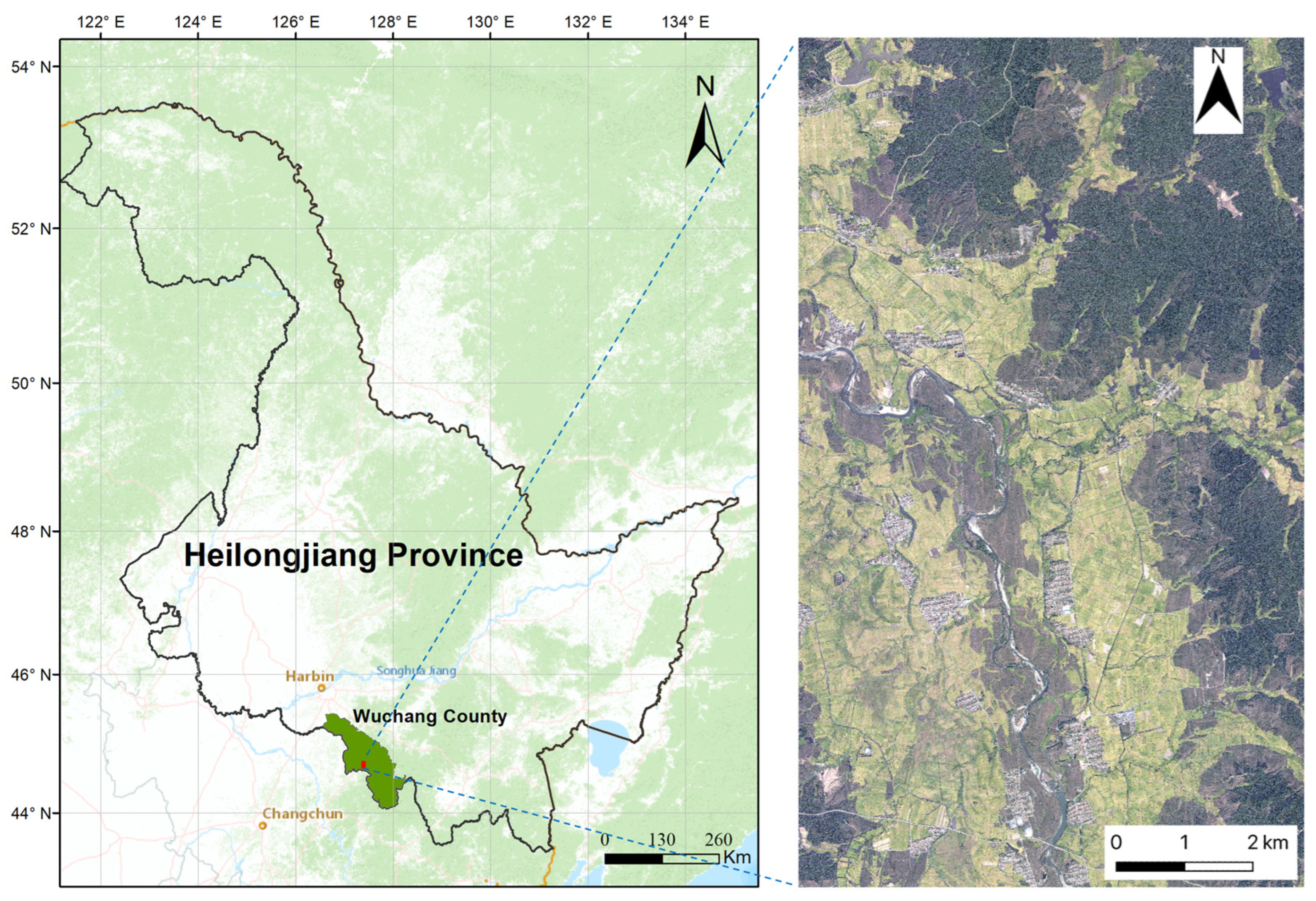
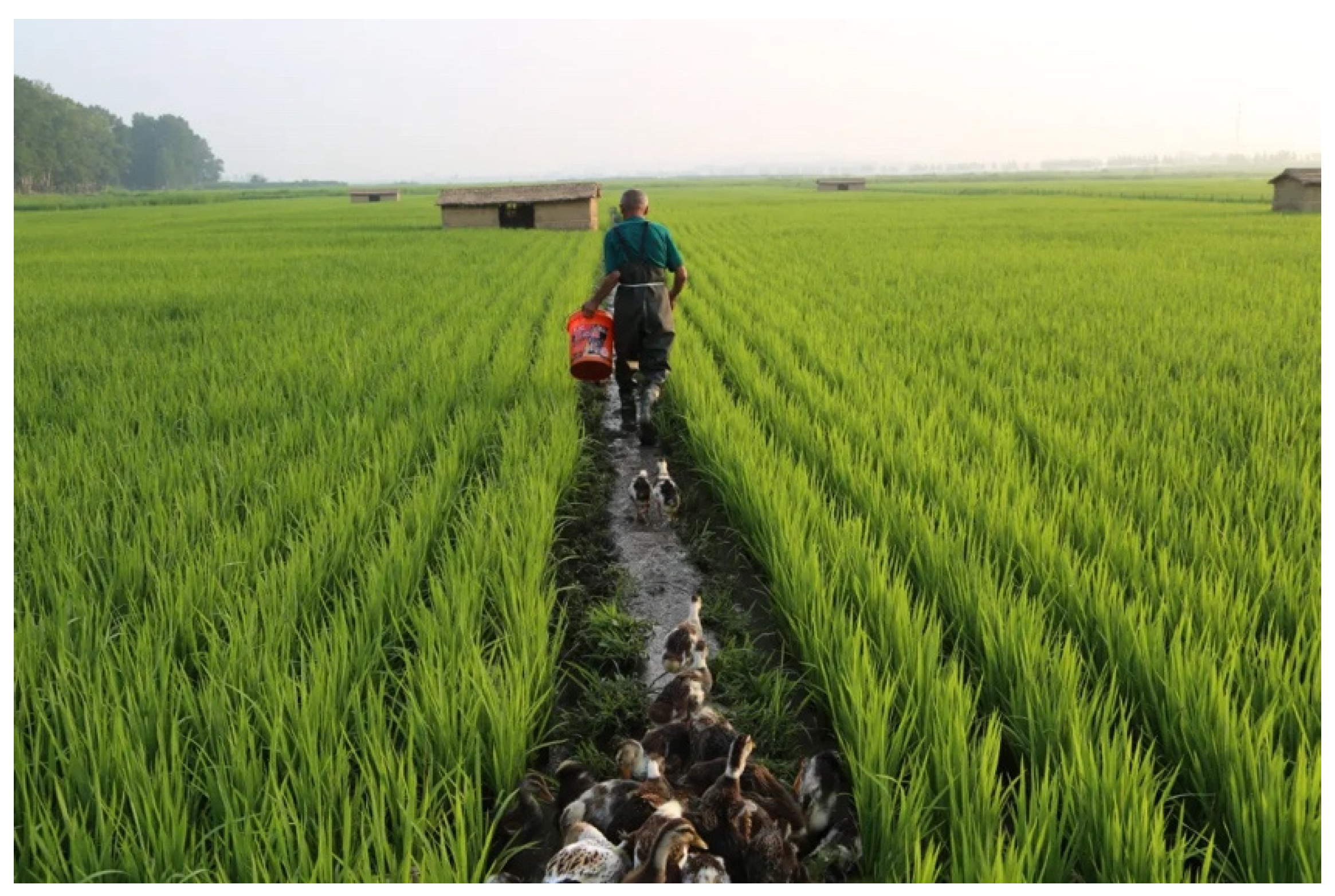
2.1. Study Area

The study area is a typical rice-planting region in Heilongjiang Province, the northmost part of China. It is a 10.5 km × 17.5 km rectangle region in Wuchang County, as shown on the maps in Figure 1. The county is famous for its high-quality japonica rice, with an approximate rice-growing area of 166,000 hectares (2021). A single rice cropping system is practiced in the area. In particular, transplanting is the predominating planting method, while very few direct seeding cases emerged in recent years. The rice-growing season starts in early May and ends in October. Figure 2 illustrates a scene showing the study area’s typical rice field boundary bank.

2.2. Data Source and Data Annotation

2.2.1. Remote Sensing Data

• Fine-resolution RGB satellite image

Fine-resolution remote sensing data are a requisite to extract field boundaries in our study case since rice field boundaries are commonly around one meter in width. Nonetheless, only the true-color RGB imagery is required for image segmentation purposes. We acquired the RGB composite of the study area from CNES/Airbus Pléiades satellite imagery captured in September 2018. The RGB image is in 20,992×35,072 pixels and 0.5 m spatial resolution.

2.

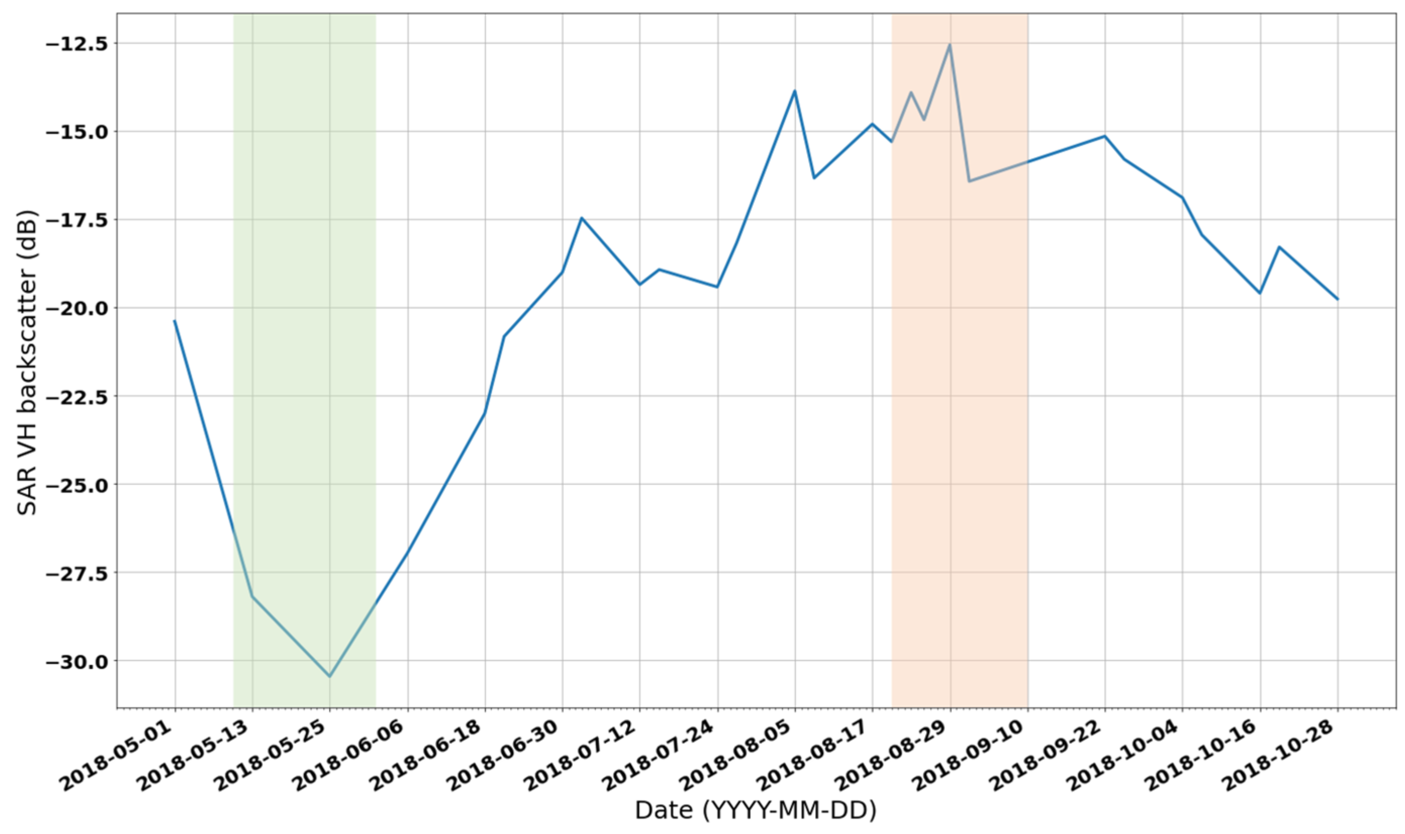
Sentinel-1 time series images

We acquired the time series of the European Space Agency (ESA) Sentinel-1 Level-1 Ground Range Detected (GRD) data product between May to October 2018 for pixel-wise rice mapping. Previous studies suggested that VH polarization has an advantage in characterizing rice growth compared to VV [31,32]. The VH band of the GRD images was derived for identifying rice field pixels. The data acquisition and processing were completed on the Google Earth Engine (GEE) cloud computing platform. The GRD data has already undergone several preprocessing steps, provided with a backscattering coefficient (σ°) in decibels (dB) value.

The Sentinel-1 two-satellite constellation has a 6-day repeat cycle. However, it should be noted that only Sentinel-1 B data were accessible. There were overlaps of orbits in the study area. Hence the number of available SAR images reached 27. Spatial resolution of the SAR images is 10 m.

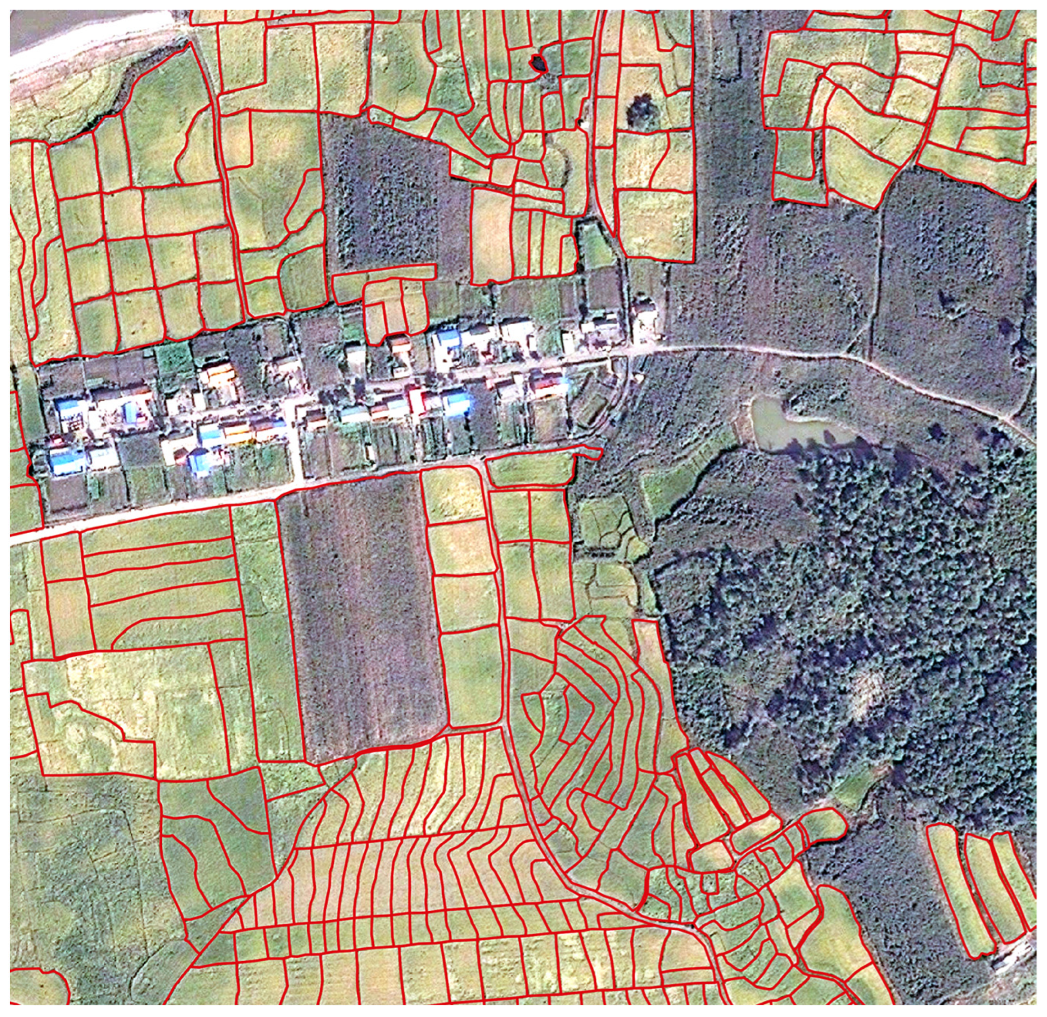
2.2.2. Agricultural Field Boundary Annotation

We selected three rectangle sampling regions on the fine-resolution RGB image to sketch agricultural field boundaries by visual interpretation (see Figure 3). With the assistance of GIS software, the three sample regions were labeled into polygons representing three landcover classes: field boundary, the agricultural field, and background landcover. The data labeling process involves the following steps:

(1) Sketch the boundaries of agriculture fields to generate field polygons by visual interpretation.

(2) Create buffers on both sides of the polygon’s edges from step (1) with a distance of 0.5 m, resulting in boundary buffers of one meter width, which is a typical distance for field boundaries for our study case.

(3) Generate agricultural field polygons (excluding the field boundary bank) by erasing the boundary buffers of step (2) from polygons from step (1).

(4) Rasterize the boundary buffers, agricultural field polygons, and the rest into a Geotiff image with different raster values (0, 1, and 2) and in the original image’s pixel size, representing field boundary, agricultural field, and background land cover, respectively.

2.2.3. Rice Field Samples

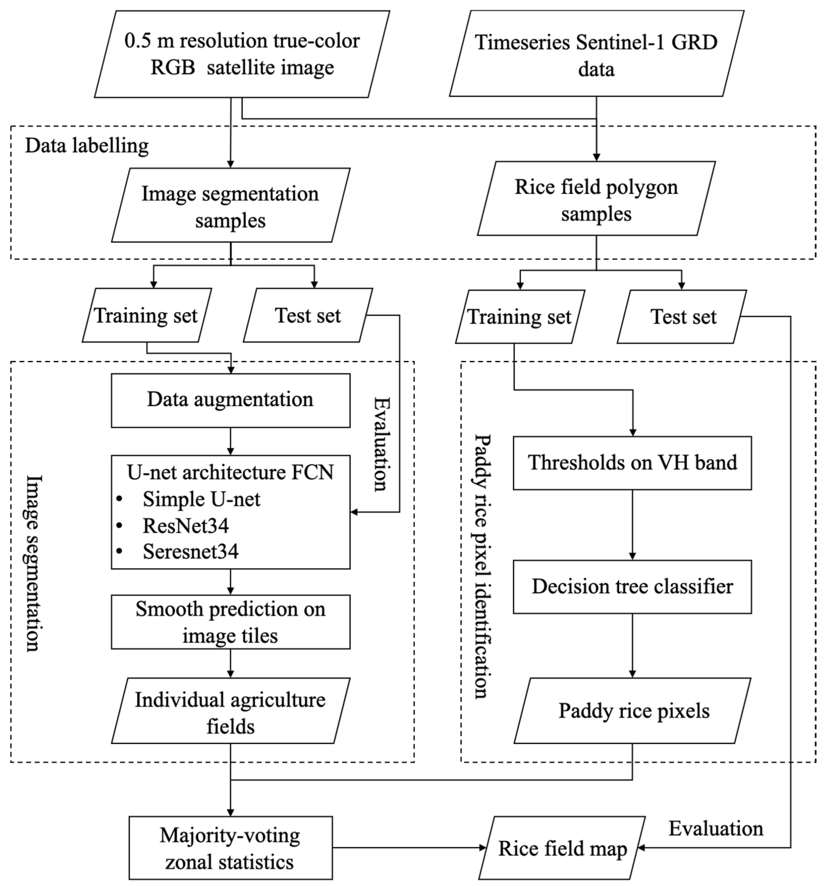
Rice is the only crop that grows in wetland conditions. The flooding signal at its early growing stage provides crucial information to identify paddy fields. We managed to label 100 rice fields based on the radar backscatter value during the rice transplanting season with the assistance of visual interpretation on the fine-resolution Pléiades satellite imagery. Half of the sample rice fields were used to determine the thresholds for a simple decision-tree classifier, and the other half was used to evaluate the final rice field mapping results.

The mean values of the VH band of GRD data from middle May to middle June (rice transplanting season) were computed on the GEE platform. Agricultural fields identified by fine-resolution image whose SAR backscatter coefficient during that period were generally low and close to the water surface were asserted as rice fields.

2.3. Methodology

The general strategy of this work is to leverage agricultural field maps to improve crop mapping. Therefore, we emphasize fine-resolution satellite image segmentation designed explicitly for agricultural field mapping. Only a simple pixel-based crop mapping classifier was required with extracted field boundaries to yield a high-resolution crop field map. The workflow of this work is illustrated in Figure 4. We first implemented the data labeling processes using a fine-resolution true-color satellite image and time series SAR images. Using the labeled data, we test three FCNs, namely a simple U-net, ResNet34-based U-net, and SeresNet34-based U-net, with different parameterizations. We applied a smooth prediction method to deal with prediction errors near the edges of image patches. Meanwhile, rice field pixels were identified with a decision-tree classifier based on phenological traits. The two outputs of field boundary extraction and rice field pixel identification were combined to produce a high-resolution rice field map.

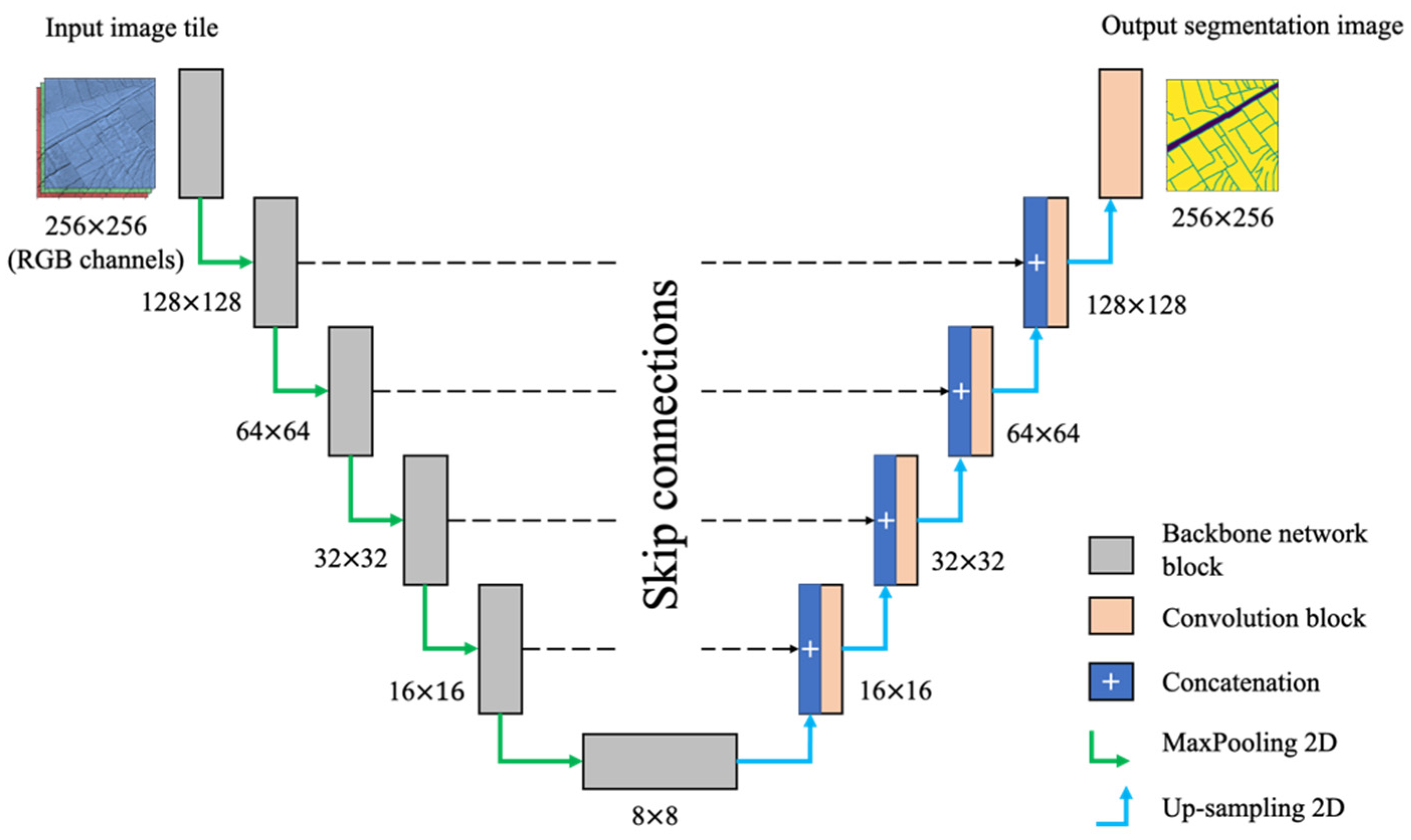
2.3.1. Image Segmentation Model

• Data preprocessing

The original RGB satellite image and the rasterized annotated target images form the training data for image segmentation. Several preprocessing steps were carried out before model training: (1) The original image and target images were clipped into 126 small patches of 256$\times$256 pixels; (2) The original RGB image channels were transformed into the range [0, 1] using the Min–Max scaler; (3) Not all image patches contain adequate field boundary pixels. We screened out those image patches whose field boundary pixels were less than 100; (4) The resulting training patches underwent data augmentation by flipping (vertically and horizontally) and rotating (at 90° intervals).

2.

U-net architecture-based CNN

The U-net is a convolutional neural network initially developed for medical image segmentation. The neural network is an improvement based on the FCN and showed its superiority with fewer training data [20]. The U-net is a CNN model of multi-scale encoders–decoders with skip connections. It has a symmetric architecture that consists of two parts: the contracting path or encoder on the left and the expansive part or decoder on the right (Figure 5). The encoder part follows the general convolutional process, which compresses the spatial information and extracts feature information while reducing the height and width of the input image. The decoder part is constituted by transposed 2D convolutional layers that upscale the encoded features and spatial information to a higher resolution pixel space to achieve a dense classification.

Many state-of-the-art CNN models have been developed in recent years for computer vision tasks, e.g., VGGNet, ResNet, DenseNet, EfficientNet, and InceptionNet. We tested the original U-net (‘simple U-net’ hereunder) by Ronneberger, Fischer, and Brox [20], ResNet34, and SeresNet34 as the backbone networks in the U-net architecture model since those are reported to be effective in satellite image segmentation tasks [21,33,34]. Each backbone network block of the simple U-net consisted of two convolution layers, a dropout layer, and a maxpooling layer. We refer to He, et al. [35], Hu, et al. [36] for details of ResNet and SerestNet, respectively. Pre-trained weights on the ImageNet dataset [37] were adopted for the backbone networks for faster and better convergence on a small training set. Parameters used to train the networks are listed (

Table 1. Parameters for training the U-net segmentation models.

Optimizer	Epochs	Loss Function	Batch Size	Metrics
Adam	150	Dice loss + Focal loss	16	Jaccard coefficient

). The image segmentation tasks were conducted using Python 3.7 language, TensorFlow 2.0, and an open-source Python library Segmentation Models (https://github.com/qubvel/segmentation_models (accessed on 12 August 2022)) on a server with Nvidia V100 graphic cards.

2.3.2. Smooth Predictions for Image Patches

The original satellite image was cropped into small patches (256$\times$256 pixels) to feed into the trained segmentation models at the prediction phase. The segmentation models make predictions solely on those small local windows of the image patch rather than the whole study area. As a result, prediction errors and conflicts near the border of the patches were not neglectable. We applied a smooth blending strategy for predicted image patches to solve this issue. First, for each image patch, the eight transformations of Dihedral Group D_4 were used, i.e., three possible 90 degree rotations and a mirrored version of those rotations and the patch itself. As a result, each patch has an eight-fold augmented prediction before merging the predictions.

While making predictions on the whole study area, the original satellite image was cropped into patches with 50% overlapping to eliminate the border effects. All the predictions for each patch were spatially merged by weighting pixels. The basic idea of merging the overlapping region is that if the pixel location is closer to the patch center, the more weight it has from that patch’s prediction. The weights are computed by interpolating with a 2-D Gaussian function. The final prediction label $L$ is defined by soft voting strategy with the following equations.

$$L=\underset{c}{\arg \max }\frac{{\sum }_i^k{w}_i\ast p_{i,c}}{k}c\in \left\{0,1,2\right\}$$

(1)

$$w_i\left(x,y\right)=e^{\frac{-x^2-y^2}{10000}}$$

(2)

Equation (1) is the voting rule for each pixel, where $w_i$ is the ith weight of prediction and $p_{i,c}$ is the ith prediction on the probability of class $c$. $w_i$ is a function of the pixel location relative to the image center as (0, 0). The weight $w_i\left(x,y\right)$ is computed by Equation (2), where (x, y) denotes the pixel’s coordinates ranging from (−127, −127) to (128, 128). $k$ is the number of predictions. Depending on pixel location on the original image, $k$ can be either 8, 16, or 32.

Following the above procedures, the image segmentation of each image patch was blended to produce a full-size segmentation result image. The resulting image then underwent several processing steps for future use in crop mapping:

(1)

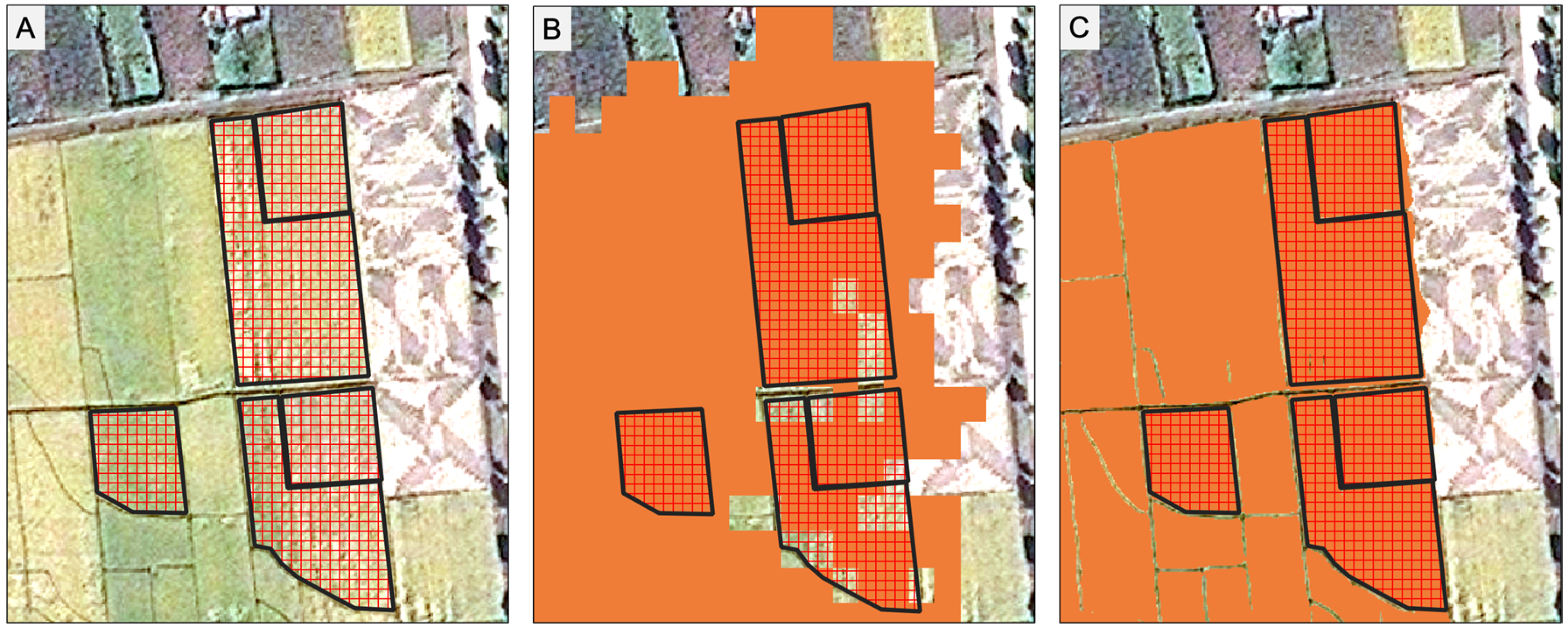
Vectorization of segmentation results in an image while keeping the topology of fields and boundaries. Connected pixels of the same class will result in an individual polygon.

(2)

Delete the boundaries from the map and keep the only agricultural field and background category for crop mapping. At this point, the boundary class was redundant information since agricultural fields were extracted.

The output vector data contain a large number of objects (polygons) of agricultural fields and background land parcels, while the field boundary bank areas were excluded.

2.3.3. Rice Field Identification

Due to the rice field’s unique wetland condition during the vegetative phase, rice fields show a unique temporal profile of radar signal compared to other landcover types. A few days before and after transplanting, the radar signal of rice fields is dominated by the water surface and is at its lowest level. The development of the rice canopy during the vegetative phase leads to a continuous increase in radar backscatter, reaching a maximum at the heading stage [38]. Based on this phenological characteristic of the radar signal, we devised a simple decision-tree classifier to discriminate between rice and non-rice pixels using Sentinel-1 SAR images. The time series of radar backscatter from Sentinel-1’s VH polarization was used to detect flooding signals at the transplanting stage and peak signals at the heading stage. Figure 6 illustrates the temporal profile of the SAR backscatter of the sample rice fields from the training set. Based on the local cropping calendar, the time window for flooding signal was set to 10 May to 01 June, and 20 August to 10 September for peak signal.

Two thresholds were fixed according to the mean pixel value (VH band) of sample rice fields from multiple SAR images during the two windows. For the flooding signal, the lower threshold was the upper quartile of sample rice pixels, i.e., −25.43 dB. For the peak signal, the upper threshold was the lower quartile −13.83 dB.

$$rice pixel=\{\begin{array}{c}flooding signal \le -25.43 dB\\ peak signal \ge -13.83 dB\end{array}$$

(3)

This simple decision-tree classifier (Equation (3)) generated a map showing rice pixels and non-rice pixels. The final step of producing a more precise rice field map is to combine the pixel-based rice map with the field boundary map resulting from satellite image segmentation. A field from the image segmentation is classified as rice or non-rice by majority voting from the pixels within its spatial extent.

2.3.4. Evaluation Metric

We used Intersection over Union (IoU) as the key metric to evaluate the image segmentation and rice field mapping results. IoU is the ratio of the overlap area to the combined area of prediction and ground truth, ranging from 0 to 1 (Equation (4)). It is equivalent to the Jaccard coefficient and is commonly used to evaluate image segmentation tasks. For the evaluation of rice field mapping in this study, IoU is a better metric than the User’s Accuracy and Producer’s Accuracy since IoU evaluates classification accuracy and spatial coherency simultaneously between test rice fields and the prediction.

$$IoU=\frac{prediciton {\cap }^{ }ground truth}{prediciton {\cup }^{ }ground truth}$$

(4)

Meanwhile, User’s Accuracy (UA, precision), Producer’s Accuracy (PA, recall), and F1 were used to evaluate pixel-wise rice identification and agricultural boundary extraction. The three metrics for class C are defined as:

$$U{A}_C=\frac{Number of correctly classified samples of C}{Sum of samples classified as C}$$

(5)

$$P{A}_C=\frac{Number of correctly classified samples of C}{Sum of samples with true lael of C}$$

(6)

$$F1=\frac{2\times U{A}_C\times P{A}_C}{U{A}_C+P{A}_C}$$

(7)

3. Results

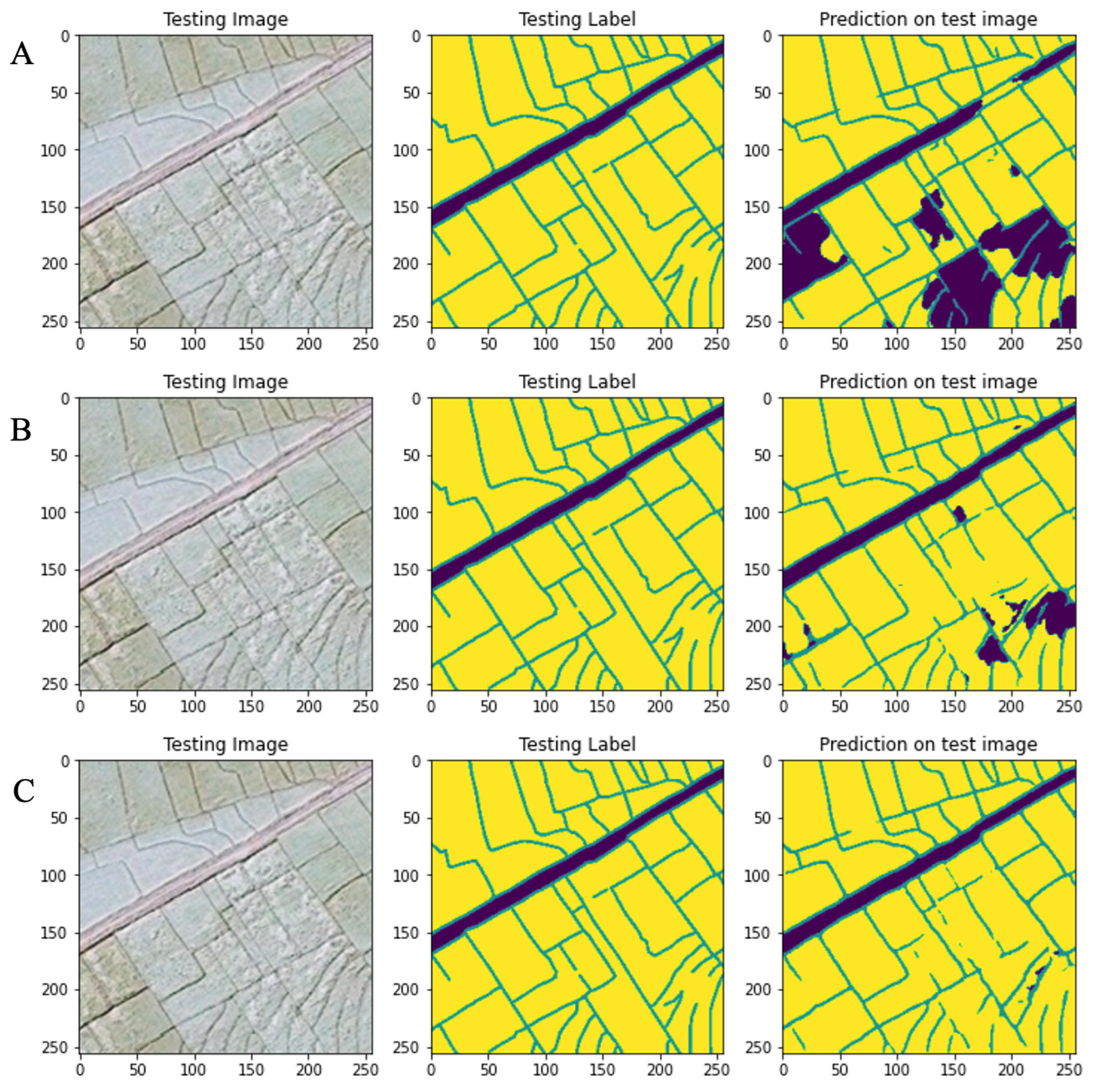
3.1. Satellite Image Segmentation Results

Evaluation on the test images shows that the U-net with SeresNet34 had the best performance, with 0.801 for IoU and 0.782 for F1 on boundary detection. The ResNet34-based U-net had an IoU of 0.755 and 0.757 for F1 on boundary detection, while the metrics for the simple U-net structure were 0.687 and 0.758, respectively (

Table 2. Evaluation scores of the three image segmentation models.

Model Backbone	IoU	User’s Accuracy on Boundary Detection	Producer’s Accuracy on Boundary Detection	F1 on Boundary Detection
Simple U-net	0.687	0.763	0.754	0.758
ResNet34	0.755	0.795	0.723	0.757
SeresNet34	0.801	0.797	0.768	0.782

). Figure 7 is a comparison of the three image segmentation models’ performance. Predictions on a test image show that simple U-net (A) and ResNet34-based U-net (B) had considerable errors in classifying agricultural fields into background land cover. SeresNet34-based U-net (C), on the other hand, overcame this problem with a higher IoU score. Nonetheless, all three models had matching performance levels detecting the field boundaries, which is our study’s most critical predicting target. Figure 8 shows the satellite image segmentation map. The map illustrates a good matching of agricultural field boundary extraction with ground truth.

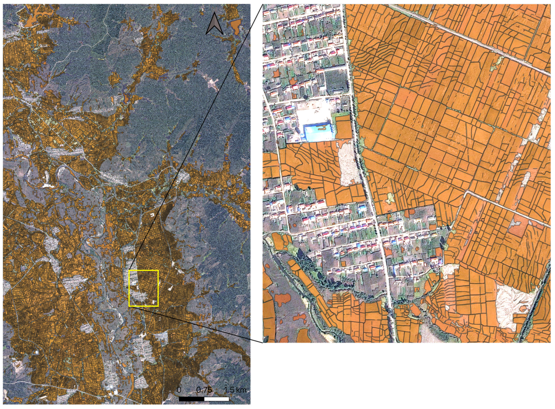
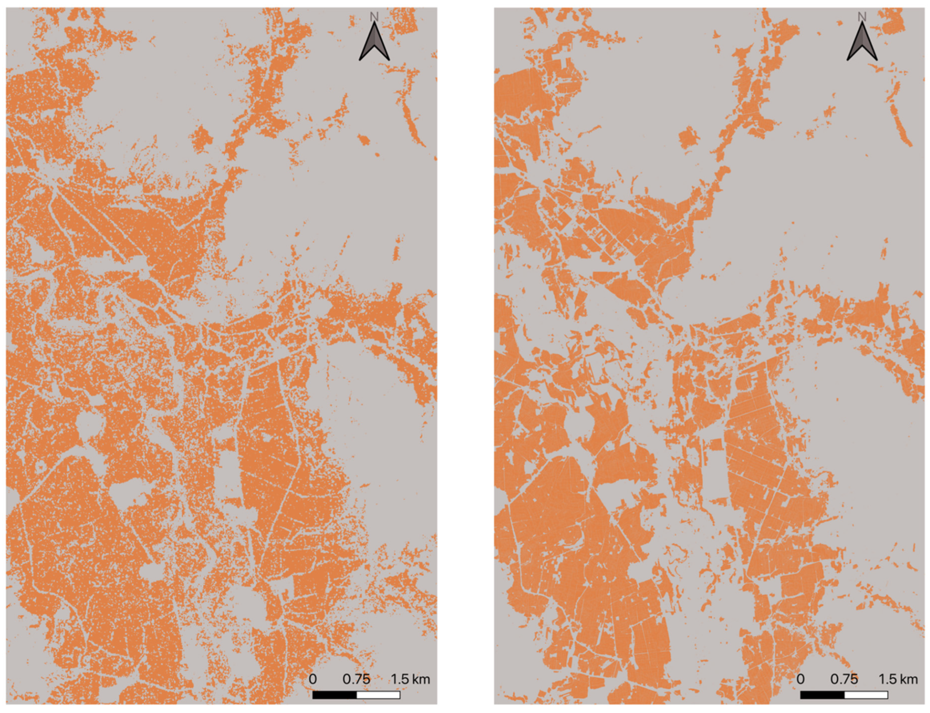
3.2. Rice Field Mapping Results

The simple decision-tree classifier produced a 10 m spatial resolution rice pixel map. However, the mixed pixel problem and the ‘salt and pepper’ effect were evident. According to the model evaluation on test data, SeresNet34 had the best overall performance for land parcel delineation, hence was used to produce the rice field map. The comparison of rice field maps (Figure 9) produced by the decision-tree classifier and by that combined with the image segmentation map proves that the combination of the two outputs tremendously improved rice field mapping in terms of the ‘salt and pepper’ effect and spatial consistency. The rice field map was assessed with the 50 rice field polygons of the test set. The IoU score reached 0.953. Pixel-wise rice field mapping was evaluated with User’s Accuracy (precision), Producer’s Accuracy (recall), and F1 which were 0.824, 0.816, and 0.820 respectively (

Table 3. Evaluations of rice field mapping results.

Model	IoU	User’s Accuracy	Producer’s Accuracy	F1
Proposed combination method	0.953	-	-	-
Pixel-wise decision-tree classifier	-	0.824	0.816	0.820

).

Figure 10 illustrates a comparison of the two rice field mapping results on some sample rice fields from the test set. The pixel-wise rice mapping was unable to distinguish the field boundaries and mixed pixel problem occurred on and around the field boundaries. Combining the two mapping results greatly improves the rice mapping precision and the mixed pixel problem with exclusion of boundary pixels.

4. Discussion

Satellite image segmentation and crop mapping are two valued areas in remote sensing application research. This study combined these two techniques to enable an OBIA on pixel-wise classification for rice field mapping. Our strategy was to use objects generated from fine-resolution image segmentation and a crop map produced by a simple pixel-wise classification model to utilize multi-source remote sensing data. Several issues and implications about this methodology should be highlighted.

The satellite image segmentation process was designed for agricultural field boundary extraction. The delineated individual agricultural field relies on the connectivity of field boundaries. Therefore, the field boundary is the foremost target for segmentation performance among the three classification targets (field, field boundary, and background). Experiments on three backbone networks presented similar F1 scores in field boundary extraction, although varied in IoU score for all three categories. The speculated reason is that field boundaries form the most prominent features for the CNN model to extract in the training process, compared to the other two categories that comprise most pixels. A higher IoU score would contribute to a more precise agricultural field map.

We noted that with many trials on the different model hyperparameters, evaluations presented slight improvement with the IoU score. A significant factor that hampered the model performance was the limited training set. The training data were manually annotated with laborious work. A larger training set is anticipated to improve the image segmentation results. It should be noted that the date of the fine-resolution has a substantial visual effect on detecting field boundaries. The image acquisition date should be chosen before the planting date or at the late phase of crop growing so that field boundaries are visually contrasting against the background.

Agricultural fields were identified based on closed field boundaries. Some of the predicted field boundaries were discontinuous, leading to the merging of multiple actual fields on the field map. The impact of the delineated field boundaries on crop mapping should be noted. The agricultural land use of this study area is dominated by rice growing. The field boundaries on the ground at our study level were mainly built for agronomic instead of cadastral purposes. The merging of several neighboring fields would have an acceptable impact on rice field mapping. However, this impact should be further investigated in a study area with complex agricultural land use.

The pixel-wise classification model for rice field detection was based on rice phenology traits. The simple decision-tree model had a mediocre performance in precision and recall scores. Combining the result with agricultural field maps generated a precise and high-resolution rice field map. Many more sophisticated pixel-wise crop mapping methods were developed using time series remote sensing data, e.g., Deep Neural Network [39,40,41,42], support vector machines [43,44,45], and Random Forest [46,47]. These pixel-wise crop mapping studies reported overall good results (0.85 or above in F1 score). However, mixed pixel and the ‘salt and pepper’ effect were inevitable in their resulting crop maps as with other pixel-wise classification tasks. On the other hand, those sophisticated pixel-wise crop mapping methods are likewise eligible to incorporate into the agricultural field map of this study to yield precise crop maps. Nonetheless, the necessity of developing those complex pixel-wise crop mapping models is debatable since the OBIA on the classified pixels was based on majority voting.

5. Conclusions

This study proposed a crop mapping framework that combines agricultural field boundary extraction with fine-resolution satellite images and pixel-wise crop detection with time series SAR imagery. We solved the prediction errors and conflicts near the border of the patches with a smooth blending strategy from multiple weighted predictions. An OBIA on the pixel-wise crop maps was employed based on majority voting to produce high-resolution crop maps.

Several conclusions can be drawn from the experiment results: (1) SeresNet34 as the backbone of the U-net model had the best performance in agricultural field extraction compared to a simple U-net and ResNet-based U-net; (2) A combination of agricultural field maps with a rice pixel detection model showed promising improvement in accuracy and resolution of rice mapping. The proposed model combination scheme only requires a simple pixel-wise crop detection model incorporating an OBIA to produce high-precision and high-resolution crop maps. This would potentially lower the cost of producing high-resolution crop maps.

References

1. Waldner, F.; Canto, G.S.; Defourny, P. Automated annual cropland mapping using knowledge-based temporal features. ISPRS J. Photogramm. Remote Sens. 2015, 110, 1–13. [Google Scholar] [CrossRef]
2. Yang, L.; Mansaray, L.R.; Huang, J.; Wang, L. Optimal segmentation scale parameter, feature subset and classification algorithm for geographic object-based crop recognition using multisource satellite imagery. Remote Sens. 2019, 11, 514. [Google Scholar] [CrossRef]
3. Peña-Barragán, J.M.; Ngugi, M.K.; Plant, R.E.; Six, J. Object-based crop identification using multiple vegetation indices, textural features and crop phenology. Remote Sens. Environ. 2011, 115, 1301–1316. [Google Scholar] [CrossRef]
4. Scharr, H. Optimal filters for extended optical flow. In International Workshop on Complex Motion; Springer: Berlin/Heidelberg, Germany, 2004; pp. 14–29. [Google Scholar]
5. Lavreniuk, M.; Kussul, N.; Shelestov, A.; Dubovyk, O.; Löw, F. Object-based postprocessing method for crop classification maps. In Proceedings of the IGARSS 2018-2018 IEEE International Geoscience and Remote Sensing Symposium, Valencia, Spain, 22–27 July 2018; pp. 7058–7061. [Google Scholar]
6. Zhang, X.; Wu, B.; Ponce-Campos, G.E.; Zhang, M.; Chang, S.; Tian, F. Mapping up-to-date paddy rice extent at 10 m resolution in china through the integration of optical and synthetic aperture radar images. Remote Sens. 2018, 10, 1200. [Google Scholar] [CrossRef]
7. Xiao, W.; Xu, S.; He, T. Mapping paddy rice with sentinel-1/2 and phenology-, object-based algorithm—A implementation in Hangjiahu plain in China using gee platform. Remote Sens. 2021, 13, 990. [Google Scholar] [CrossRef]
8. Li, Q.; Wang, C.; Zhang, B.; Lu, L. Object-based crop classification with Landsat-MODIS enhanced time-series data. Remote Sens. 2015, 7, 16091–16107. [Google Scholar] [CrossRef]
9. Song, Q.; Hu, Q.; Zhou, Q.; Hovis, C.; Xiang, M.; Tang, H.; Wu, W. In-season crop mapping with GF-1/WFV data by combining object-based image analysis and random forest. Remote Sens. 2017, 9, 1184. [Google Scholar] [CrossRef]
10. Peña, J.M.; Gutiérrez, P.A.; Hervás-Martínez, C.; Six, J.; Plant, R.E.; López-Granados, F. Object-based image classification of summer crops with machine learning methods. Remote Sens. 2014, 6, 5019–5041. [Google Scholar] [CrossRef]
11. Liu, X.; Bo, Y. Object-based crop species classification based on the combination of airborne hyperspectral images and LiDAR data. Remote Sens. 2015, 7, 922–950. [Google Scholar] [CrossRef]
12. Tang, Z.; Wang, H.; Li, X.; Li, X.; Cai, W.; Han, C. An object-based approach for mapping crop coverage using multiscale weighted and machine learning methods. IEEE J. Sel. Top. Appl. Earth Obs. Remote Sens. 2020, 13, 1700–1713. [Google Scholar] [CrossRef]
13. Clauss, K.; Ottinger, M.; Künzer, C. Mapping rice areas with Sentinel-1 time series and superpixel segmentation. Int. J. Remote Sens. 2018, 39, 1399–1420. [Google Scholar] [CrossRef]
14. Li, D.; Zhang, G.; Wu, Z.; Yi, L. An edge embedded marker-based watershed algorithm for high spatial resolution remote sensing image segmentation. IEEE Trans. Image Process. 2010, 19, 2781–2787. [Google Scholar] [PubMed]
15. Xue, Y.; Zhao, J.; Zhang, M. A watershed-segmentation-based improved algorithm for extracting cultivated land boundaries. Remote Sens. 2021, 13, 939. [Google Scholar] [CrossRef]
16. Waldner, F.; Diakogiannis, F.I. Deep learning on edge: Extracting field boundaries from satellite images with a convolutional neural network. Remote Sens. Environ. 2020, 245, 111741. [Google Scholar] [CrossRef]
17. Rawat, W.; Wang, Z. Deep convolutional neural networks for image classification: A comprehensive review. Neural Comput. 2017, 29, 2352–2449. [Google Scholar] [CrossRef]
18. Krizhevsky, A.; Sutskever, I.; Hinton, G.E. Imagenet classification with deep convolutional neural networks. Commun. ACM. 2017, 60, 84–90. [Google Scholar] [CrossRef]
19. Long, J.; Shelhamer, E.; Darrell, T. Fully convolutional networks for semantic segmentation. In Proceedings of the IEEE Conference on Computer Vision and Pattern Recognition, Boston, MA, USA, 7–12 June 2015; pp. 3431–3440. [Google Scholar]
20. Ronneberger, O.; Fischer, P.; Brox, T. U-Net: Convolutional Networks for Biomedical Image Segmentation. In Proceedings of the Medical Image Computing and Computer-Assisted Intervention—MICCAI 2015, Munich, Germany, 5–9 October 2015; pp. 234–241. [Google Scholar]
21. Garcia-Pedrero, A.; Lillo-Saavedra, M.; Rodriguez-Esparragon, D.; Gonzalo-Martin, C. Deep learning for automatic outlining agricultural parcels: Exploiting the land parcel identification system. IEEE Access 2019, 7, 158223–158236. [Google Scholar] [CrossRef]
22. Masoud, K.M.; Persello, C.; Tolpekin, V.A. Delineation of agricultural field boundaries from Sentinel-2 images using a novel super-resolution contour detector based on fully convolutional networks. Remote Sens. 2019, 12, 59. [Google Scholar] [CrossRef]
23. Farooq, A.; Jia, X.; Hu, J.; Zhou, J. Multi-resolution weed classification via convolutional neural network and superpixel based local binary pattern using remote sensing images. Remote Sens. 2019, 11, 1692. [Google Scholar] [CrossRef]
24. Li, H.; Zhang, C.; Zhang, Y.; Zhang, S.; Ding, X.; Atkinson, P.M. A Scale Sequence Object-based Convolutional Neural Network (SS-OCNN) for crop classification from fine spatial resolution remotely sensed imagery. Int. J. Digit. Earth 2021, 14, 1528–1546. [Google Scholar] [CrossRef]
25. Zhang, X.; Wang, Q.; Chen, G.; Dai, F.; Zhu, K.; Gong, Y.; Xie, Y. An object-based supervised classification framework for very-high-resolution remote sensing images using convolutional neural networks. Remote Sens. Lett. 2018, 9, 373–382. [Google Scholar] [CrossRef]
26. Tian, S.; Lu, Q.; Wei, L. Multiscale Superpixel-Based Fine Classification of Crops in the UAV-Manned Hyperspectral Imagery. Remote Sens. 2022, 14, 3292. [Google Scholar] [CrossRef]
27. Chen, Q.; Cao, W.; Shang, J.; Liu, J.; Liu, X. Superpixel-Based Cropland Classification of SAR Image With Statistical Texture and Polarization Features. IEEE Geosci. Remote Sens. Lett. 2021, 19, 1–5. [Google Scholar] [CrossRef]
28. Zhu, X.X.; Tuia, D.; Mou, L.; Xia, G.-S.; Zhang, L.; Xu, F.; Fraundorfer, F. Deep learning in remote sensing: A comprehensive review and list of resources. IEEE Geosci. Remote Sens. Mag. 2017, 5, 8–36. [Google Scholar] [CrossRef]
29. Liu, S.; Ding, W.; Liu, C.; Liu, Y.; Wang, Y.; Li, H. ERN: Edge loss reinforced semantic segmentation network for remote sensing images. Remote Sens. 2018, 10, 1339. [Google Scholar] [CrossRef]
30. Mohammadimanesh, F.; Salehi, B.; Mahdianpari, M.; Gill, E.; Molinier, M. A new fully convolutional neural network for semantic segmentation of polarimetric SAR imagery in complex land cover ecosystem. ISPRS J. Photogramm. Remote Sens. 2019, 151, 223–236. [Google Scholar] [CrossRef]
31. Lasko, K.; Vadrevu, K.P.; Tran, V.T.; Justice, C. Mapping double and single crop paddy rice with Sentinel-1A at varying spatial scales and polarizations in Hanoi, Vietnam. IEEE J. Sel. Top. Appl. Earth Obs. Remote Sens. 2018, 11, 498–512. [Google Scholar] [CrossRef]
32. Nguyen, D.B.; Gruber, A.; Wagner, W. Mapping rice extent and cropping scheme in the Mekong Delta using Sentinel-1A data. Remote Sens. Lett. 2016, 7, 1209–1218. [Google Scholar] [CrossRef]
33. Buslaev, A.; Seferbekov, S.; Iglovikov, V.; Shvets, A. Fully convolutional network for automatic road extraction from satellite imagery. In Proceedings of the IEEE Conference on Computer Vision and Pattern Recognition Workshops, Salt Lake City, UT, USA, 18–23 June 2018; pp. 207–210. [Google Scholar]
34. Qayyum, N.; Ghuffar, S.; Ahmad, H.M.; Yousaf, A.; Shahid, I. Glacial lakes mapping using multi satellite PlanetScope imagery and deep learning. ISPRS Int. J. Geo-Inf. 2020, 9, 560. [Google Scholar] [CrossRef]
35. He, K.; Zhang, X.; Ren, S.; Sun, J. Deep residual learning for image recognition. In Proceedings of the IEEE Conference on Computer Vision and Pattern Recognition, Las Vegas, NV, USA, 27–30 June 2018; pp. 770–778. [Google Scholar]
36. Hu, J.; Shen, L.; Sun, G. Squeeze-and-excitation networks. In Proceedings of Proceedings of the IEEE Conference on Computer Vision and Pattern Recognition, Salt Lake City, UT, USA,, 18–23 June 2018; pp. 7132–7141. [Google Scholar]
37. Deng, J.; Dong, W.; Socher, R.; Li, L.-J.; Li, K.; Li, F.-F. Imagenet: A large-scale hierarchical image database. In Proceedings of the 2009 IEEE Conference on Computer Vision and Pattern Recognition, Miami, FL, USA, 20–25 June 2009; pp. 248–255. [Google Scholar]
38. Chen, C.; McNairn, H. A neural network integrated approach for rice crop monitoring. Int. J. Remote Sens. 2006, 27, 1367–1393. [Google Scholar] [CrossRef]
39. Qu, Y.; Zhao, W.; Yuan, Z.; Chen, J. Crop mapping from sentinel-1 polarimetric time-series with a deep neural network. Remote Sens. 2020, 12, 2493. [Google Scholar] [CrossRef]
40. Kussul, N.; Lavreniuk, M.; Skakun, S.; Shelestov, A. Deep learning classification of land cover and crop types using remote sensing data. IEEE Geosci. Remote Sens. Lett. 2017, 14, 778–782. [Google Scholar] [CrossRef]
41. Zhang, M.; Lin, H.; Wang, G.; Sun, H.; Fu, J. Mapping paddy rice using a convolutional neural network (CNN) with Landsat 8 datasets in the Dongting Lake Area, China. Remote Sens. 2018, 10, 1840. [Google Scholar] [CrossRef]
42. Wang, M.; Wang, J.; Chen, L. Mapping paddy rice using weakly supervised long short-term memory network with time series sentinel optical and SAR Images. Agriculture 2020, 10, 483. [Google Scholar] [CrossRef]
43. Hu, Q.; Sulla-Menashe, D.; Xu, B.; Yin, H.; Tang, H.; Yang, P.; Wu, W. A phenology-based spectral and temporal feature selection method for crop mapping from satellite time series. Int. J. Appl. Earth Obs. Geoinf. 2019, 80, 218–229. [Google Scholar] [CrossRef]
44. Küçük, Ç.; Taşkın, G.; Erten, E. Paddy-rice phenology classification based on machine-learning methods using multitemporal co-polar X-band SAR images. IEEE J. Sel. Top. Appl. Earth Obs. Remote Sens. 2016, 9, 2509–2519. [Google Scholar] [CrossRef]
45. Park, S.; Im, J.; Park, S.; Yoo, C.; Han, H.; Rhee, J. Classification and mapping of paddy rice by combining Landsat and SAR time series data. Remote Sens. 2018, 10, 447. [Google Scholar] [CrossRef]
46. Bazzi, H.; Baghdadi, N.; El Hajj, M.; Zribi, M.; Minh, D.H.T.; Ndikumana, E.; Courault, D.; Belhouchette, H. Mapping paddy rice using Sentinel-1 SAR time series in Camargue, France. Remote Sens. 2019, 11, 887. [Google Scholar] [CrossRef]
47. Teluguntla, P.; Thenkabail, P.S.; Oliphant, A.; Xiong, J.; Gumma, M.K.; Congalton, R.G.; Yadav, K.; Huete, A. A 30-m landsat-derived cropland extent product of Australia and China using random forest machine learning algorithm on Google Earth Engine cloud computing platform. ISPRS J. Photogramm. Remote Sens. 2018, 144, 325–340. [Google Scholar] [CrossRef]
Figure 1. The location of the study area (left) and its true-color RGB composite (right) from CNES/Airbus Pléiades satellite imagery captured in September 2018.
Agronomy 12 02342 g001
Figure 2. A picture obtained in the study area shows a typical rice field boundary bank, around 1 m in width.
Agronomy 12 02342 g002
Figure 3. A portion of field boundary annotation on the fine-resolution satellite image (0.5 m spatial resolution).
Agronomy 12 02342 g003
Figure 4. The workflow of the proposed method that combines image segmentation and pixel-based classification for high-resolution rice field mapping.
Agronomy 12 02342 g004
Figure 5. The U-net model for satellite image segmentation. The left part is backbone network blocks with skip connections to the decoder part on the right. Input is the 256 × 256 pixels of RGB channels, and output is predictions of three classes representing the agricultural field, field boundary, and background.
Agronomy 12 02342 g005
Figure 6. Temporal SAR backscatter profile (VH polarization) of sample rice fields. The green zone (10 May to 1 June) is the time window for the flooding signal and the orange zone (20 August to 10 September) for the peak signal.
Agronomy 12 02342 g006
Figure 7. Field boundary detection results on a test image by the simple U-net (A), ResNet34-based U-net (B), and SeresNet34-based U-net (C). Yellow area denotes agricultural field, blue area denotes background land cover, and green area denotes field boundary.
Agronomy 12 02342 g007
Figure 8. Agricultural field map produced by SeresNet34-based U-net image segmentation model.
Agronomy 12 02342 g008
Figure 9. Rice field (orange area) maps produced by the simple decision-tree classifier with Sentinel-1 SAR imagery (left) and by that combined with agriculture field boundary delineation by the SeresNet34-based U-net image segmentation model (right).
Agronomy 12 02342 g009
Figure 10. Evaluation by the test set for rice field mapping: (A) sample rice fields in test set, (B) sample rice fields overlay with pixel-wise classification by decision-tree classifier, and (C) sample rice fields overlay with rice field map produced by the proposed method.
Agronomy 12 02342 g010