Recognition of Areca Leaf Yellow Disease Based on PlanetScope Satellite Imagery

Abstract

Areca yellow leaf disease is a major attacker of the planting and production of arecanut. The continuous expansion of arecanut (Areca catechu L.) planting areas in Hainan has placed a great need to strengthen the monitoring of this disease. At present, there is little research on the monitoring of areca yellow leaf disease. PlanetScope imagery can achieve daily global coverage at a high spatial resolution (3 m) and is thus suitable for the high-precision monitoring of plant pest and disease. In this paper, PlanetScope images were employed to extract spectral features commonly used in disease, pest and vegetation growth monitoring for primary models. In this paper, 13 spectral features commonly used in vegetation growth and pest monitoring were selected to form the initial feature space, followed by the implementation of the Correlation Analysis (CA) and independent t-testing to optimize the feature space. Then, the Random Forest (RF), Backward Propagation Neural Network (BPNN) and AdaBoost algorithms based on feature space optimization to construct double-classification (healthy, diseased) monitoring models for the areca yellow leaf disease. The results indicated that the green, blue and red bands, and plant senescence reflectance index (PSRI) and enhanced vegetation index (EVI) exhibited highly significant differences and strong correlations with healthy and diseased samples. The RF model exhibits the highest overall recognition accuracy for areca yellow leaf disease (88.24%), 2.95% and 20.59% higher than the BPNN and AdaBoost models, respectively. The commission and omission errors were lowest with the RF model for both healthy and diseased samples. This model also exhibited the highest Kappa coefficient at 0.765. Our results exhibit the feasible application of PlanetScope imagery for the regional large-scale monitoring of areca yellow leaf disease, with the RF method identified as the most suitable for this task. Our study provides a reference for the monitoring, a rapid assessment of the area affected and the management planning of the disease in the agricultural and forestry industries.

1. Introduction

Arecanut is a major economic crop in the tropical and subtropical regions of China. The continuous and rapid development of the arecanut cultivation industry has increased its cultivation area, enhancing the problems associated with arecanut disease hazards [1]. Areca yellow leaf disease is the most important factor harming arecanut production and planting. The occurrence of yellow leaf disease leads to the retarded growth and potential withering of arecanut, resulting in a huge loss of production. It reduces the yield as much as 50% over a period of 3 years immediately following disease incidence. Foliar yellowing, the most conspicuous symptom, begins from the inner whorl and spreads to the outer parts of the crown [2]. There is no direct and effective agent for the eradication of areca yellow leaf disease, and it should be cut down in time to prevent the spread once it is found. Thus, this disease is the principle limiting factor of arecanut production and cultivation [3]. The continuous occurrence of areca yellow leaf disease and the obvious decline of the industrial benefits of arecanut have highlighted the urgent need of a method that timely and accurately detects the areca yellow leaf disease. In particular, the real-time monitoring of yellow leaf disease over large areas facilitates its early prevention and control, which is key to improving the yield of arecanut and reducing the related economic losses. Current conventional monitoring, forecasting, prevention and control approaches of areca yellow leaf disease is relatively traditional. Such approaches generally focus on point-measurements, while large-scale monitoring and reporting methods are lacking [4]. This consequently has negative impacts on the prevention and control of the disease. Furthermore, traditional manual survey methods are time-consuming, labor-intensive, inaccurate, and can cause varying degrees of damage to crops.

With the continuous development of remote sensing technology, satellite remote sensing data sources have become more abundant. In recent decades, numerous studies have performed the “face” monitoring of the occurrence and severity of diseases and pests. Zhang et al. [5] employed band reflectance information of thematic mapper (TM) images to analyze the relationship between the severity of wheat puccinia striiformis and the corresponding spectral features to build a spectral database for the monitoring of wheat puccinia striiformis. High temporal resolution multispectral satellite images were used by Franke et al. [6] to construct a decision tree for the monitoring of wheat diseases via mixed tuned matched filtering (MTMF) and the normalized vegetation index (NDVI), with promising results for the early detection of crop infections. Tang et al. [7] combined multi-temporal HJ-CCD optical data and HJ-IRS thermal infrared data to optimize winter wheat growth factors (e.g., vegetation indices, environmental factors and land surface temperature (LST)) and input the results into a Relevance Vector Machine (RVM) to predict aphid occurrence at the grain-filling stage. Ma et al. [8] screened feature variables via the minimum redundancy maximum relevance (mRMR) and correlation analysis (CA) algorithms using Landsat8 imagery. These features were then combined with the AdaBoost algorithm, Fisher linear discriminant analysis (FLDA) and support vector machines (SVM) to construct a monitoring model for the severity of wheat powdery mildew. Results demonstrate the superiority of the combined mRMR feature selection and AdaBoost algorithm for the accurate modeling and monitoring of wheat powdery mildew. Yuan et al. [9] used a high-resolution SPOT-6 imagery to perform sensitivity analysis via mutual correlation and independent sample t-tests. The feature variables of wheat powdery mildew were then screen for a winter wheat powdery mildew inverse model using an artificial neural network (ANN), the Maximum Likelihood Estimate (MLE) and Mahalanobis distance. Despite the great progress made by the aforementioned research, the studies generally focus on field crops such as wheat, while the remote sensing monitoring of areca yellow leaf disease is limited in some regions (i.e., the tropical and subtropical regions) with fragmented plots and cloudy and rainy weather.

With the development of remote sensing technology, the high-resolution PlanetScope satellite cluster can achieve daily global coverage with a 3 m spatial resolution, providing an effective data source for the extraction of agricultural and forestry planting information in tropical and subtropical regions [10,11,12,13]. In order to overcome this limitation, in the current paper, we employ images collected from PlanetScope to perform the large-scale monitoring of areca yellow leaf disease.

The objectives of this research were to: (1) establish a high-precision areca yellow leaf disease recognition model based on feature variables optimization, which is composed of spectral features extracted from PlanetScope satellite images, (2) and evaluate the performance of three algorithms with random forest (RF), BP neural network (BPNN), and AdaBoost algorithms combined with the optimized feature variables in an attempt to identify the areca yellow leaf disease. The results provide a reference for the regional large-scale monitoring and prevention of areca yellow leaf disease.

2. Materials and Methods

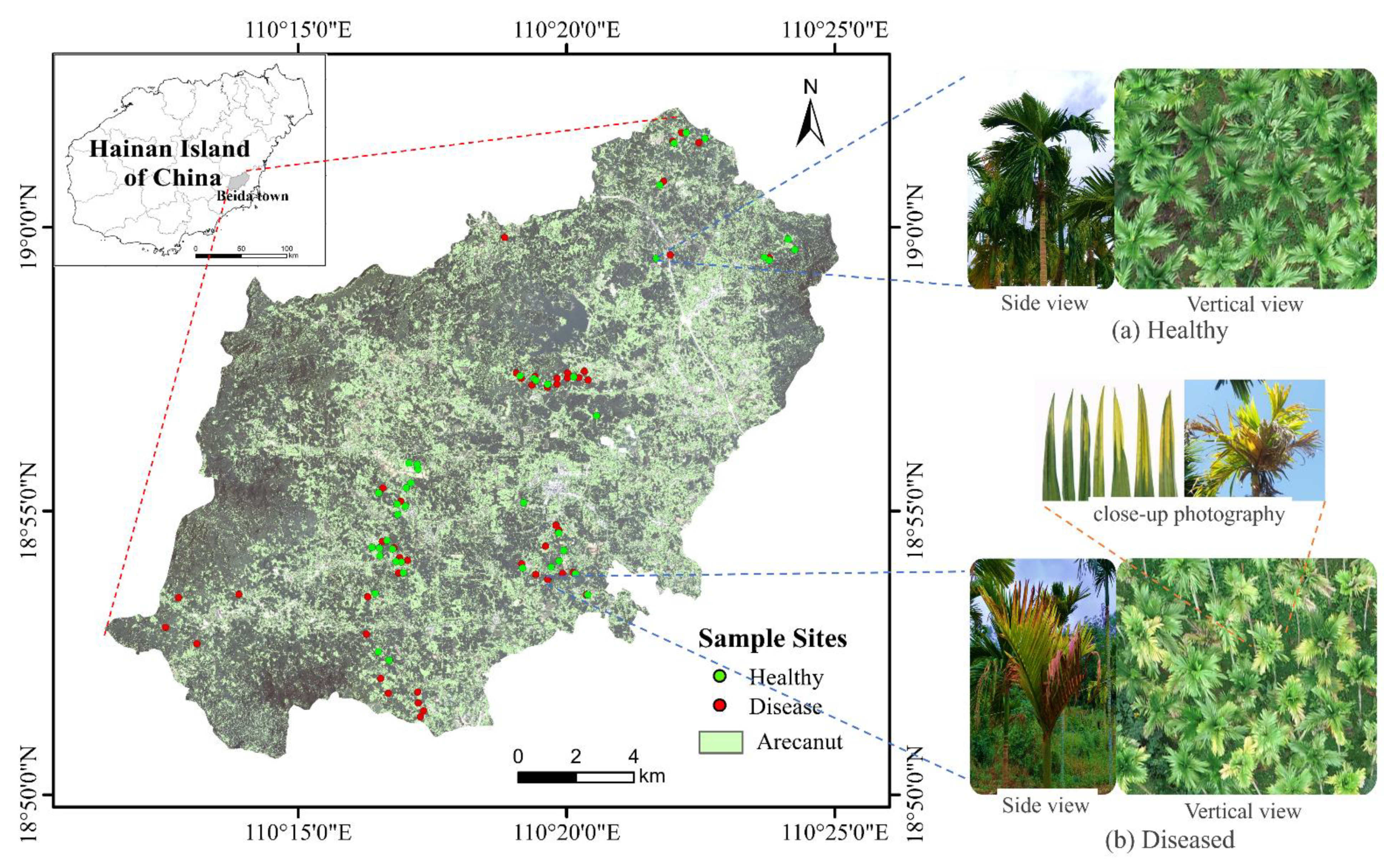
2.1. Study Area

The study area is located in Beida Town, Wanning County, Hainan Province of China (110°23′–110°40′ E, 18°86′–19°01′ N), covering a total area of 276.09 km², (Figure 1). This region is located in a hilly mountain area with a tropical monsoon climate. The annual average temperature, monthly average temperature, annual precipitation, and average annual sunshine hours are 23.6 °C, 18.7–28.5 °C, 2200 cm, and $>$1800 h, respectively. Red and sandy loam are the typical soils of the region.

Wanning County is one of the main arecanut producing areas in China. In 2019, the planting of arecanut area reached 18,138 ha, accounting for 16.4% of the planting area in Hainan [14]. Arecanut is a perennial medicinal plant of palm family, and is the first of the four major southern medicines in China. The main threat to arecanut planting and production in the region is areca yellow leaf disease. The arecanut plant height was about 10–15m, the leaf clustered at stem apex, and the leaf length was about 1.3–2.0 m. The planting distance was 2.0 m by 2.5 m with a planting density of 1500 plants per hectare. It is reported that the average incidence rate of areca yellow leaf disease in southern Wanning in 2018 reached 39.6% [15].

2.2. Data Acquisition and Processing

2.2.1. Ground Sample Data Collection

Ground sample data were obtained through field surveys on 19–21 March 2019. Considering the pixels size of remote sensing images, uniformly growing arecanut plant were randomly selected with a continuous area of 3 × 3 m, and the severity of disease was surveyed. The center coordinate of each sample was recorded by a differential global positioning system (GPS) sensor (Trimble GeoXH). The classification standard adopted in this paper was based on the percent of the yellowing leaf area to the total leaf area of the plant in continuous area of 3 × 3 m. If the percent of the yellowing leaf area to the total leaf area of the plant was less than 1%, the plant was considered to be healthy. Otherwise, it was considered to be diseased. Finally, A total of 94 field survey samples were determined (Figure 1). This survey sample dataset was divided into two sub-datasets, the health dataset (47 survey samples) and the disease dataset (47 survey samples), to identify the arecanut planting areas infected with yellowing disease. Two thirds of the field survey sample points (60 survey samples) are randomly selected for modeling, and the remaining third (34 survey samples) was used to verify the model. In addition, there were 30 healthy samples and 30 diseased samples used for modeling, there were 17 healthy samples and 17 diseased samples used to verify the model.

2.2.2. Satellite Remote Sensing Imagery Acquisition

The Hainan region enjoys a cloudy and rainy climate all year round, and has complex and diverse terrain. The vegetation is evergreen, with a high degree of plot fragmentation and small area, thus making it difficult to obtain high-quality multi-temporal remote sensing images. In this situation, the extraction of high-precision fruit forest information and vegetation change monitoring require high-resolution images [16]. The cloudless PlanetScope imagery collected on 21 March 2019 was used to carry out research on the identification method of areca yellow leaf disease in this study. The Planet images were acquired by PLANET Technology Corporation (America) [17], which has the largest number of satellites in orbit across the world (currently 200 satellites). Its ultra-high frequency time resolution allows for global daily coverage. PlanetScope imaging products are the only commercial satellite imagery available with coverage, high resolution and frequency at the global scale. Planet imagery exhibits high data coverage efficiency and autonomous image coverage, with the ability to perform all-weather earth observation. As the world’s largest group of micro-satellites, the images play a key role in the monitoring of major crop diseases and pests. The image has a spatial resolution of 3 m and contains four bands in the blue, green, red and near infrared spectral regions. The Planet image selected in the study is an orthographic data product (3B) that has undergone sensor and radiometric calibration, as well as orthorectification and atmospheric correction.

Table 1. Key parameters of the PlanetScope.

Parameter	Parameter Value
Track height	International space station orbit 400 km Sun-synchronous orbit 475 km
Orbital inclination	52° 98°
Sensor type	Bayer filter CCD camera
Width	24.6 km × 16.4 km
Spatial resolution	3–4 m
Spectral band	Band1: Blue (455–515 nm) Band2: Green (500–590 nm) Band3: Red (590–670 nm) Band4: NIR (780–860 nm)

reports specific parameter information of the PlanetScope.

2.3. Sensitive Feature Variable Extraction

Vegetation indices and spectral bands were determined based on the difference in reflectance and absorption rate of plants across different spectral bands within the visible (red, green, blue bands) and near-infrared bands of the PlanetScope image in order to obtain information about plant features. We initially selected 13 spectral features commonly used for the monitoring of vegetation growth, crop diseases and pests based on the pre-processed Planet image. These features, which are related to arecanut growth and stress, were extracted as the primary feature subset (

Table 2. Selected spectral features.

Spectral Features	Formula	Reference
Blue band reflectance (Blue)	RB	[18]
Green band reflectance (Green)	RG	[18]
Red band reflectance (Red)	RR	[19]
NIR reflectance (NIR)	RNIR	[19]
Ratio vegetation index (RVI)	$R_{NIR}/R_R$	[20]
Normalized difference vegetation Index (NDVI)	$(R_{NIR}-R_R)/(R_{NIR}+R_R)$	[21]
Normalized pigment chlorophyll index (NPCI)	$\left(R_R-R_B\right)/\left(R_R+R_B\right)$	[22]
Enhanced vegetation index (EVI)	$2.5(R_{NIR}-R_R)/\left(R_{NIR}+6R_R-7.5R_B+1\right)$	[23]
Modified soil adjusted vegetation index (MSAVI)	$\frac{1}{2}[\left(2R_{NIR}+1\right)-\sqrt{{\left(2R_{NIR}+1\right)}^2-8\left(R_{NIR}-R_R\right)}]$	[24]
Plant senescence reflectance index (PSRI)	$\left(R_R-R_B\right)/R_{NIR}$	[25]
Soil-adjusted vegetation index (SAVI)	$1.5\left(R_{NIR}-R_R\right)/\left(R_{NIR}+R_R+0.5\right)$	[26]
Optimization of soil regulatory vegetation index (OSAVI)	$\left(R_{NIR}-R_R\right)/\left(R_{NIR}+R_R+0.16\right)$	[27]
Triangular vegetation index (TVI)	$60\left(R_{NIR}-R_G\right)-100\left(R_R-R_G\right)$	[28]

Note: R_R, R_G, R_B, and R_NIR are the red, green, blue and near-infrared bands, respectively.

).

2.4. Model Building Method

2.4.1. RF Algorithm Model

The Random Forest (RF) algorithm, which was initially proposed by Breiman and AdeleCulter, is an algorithm that integrates multiple trees through ensemble learning. The framework is centered around a decision tree, which is essentially a combined classification algorithm based on ensemble learning [29,30]. RF has a strong tolerance to noise, is able to handle high-dimensional data, and is less likely to exhibit over-fitting, resulting in its common application in classification and feature selection algorithms.

RF classification can generally be divided into the following steps: (1) The bootstrap method performs random sampling, where replacement is performed n times from the sample set and s samples are drawn for each sampling to obtain n training sets; (2) n new training set models are built, resulting in n decision tree models; (3) and a random decision tree is formed from the generated decision tree models, and the final prediction result is determined by the voting results of multiple tree classifiers [31]. More specifically, multiple decision trees are constructed during the training phase, and the final output is a single decision tree.

We selected the RF method to construct a remote sensing monitoring model of areca yellow leaf disease for the double-classification problem (health, disease) of areca yellow leaf disease. The implementation process is described as follows:

(1)

Dataset input. The 94 ground samples were divided into 60 and 34 samples for training set trainA and validation set testB, with training and verification labels labelA and labelB, respectively.

(2)

Parameter setting. The number of decision trees were set to 500. When the number of decision trees is more than 500, the error is generally stable and over-fitting does not occur. Other parameter values were taken as the system default.

(3)

Training and prediction. Factor = TreeBagger (n, trainA, lableA) was adopted to construct a decision and [Predict_lable, Scores] = predict (Factor, testB) for testing.

2.4.2. BPNN Algorithm Model

The Back Propagation Neural Network (BPNN) is currently the most widely used neural network. It is a multilayer feed forward neural network that trains the model through the back propagation algorithm [32]. The gradient descent method is employed to minimize the mean-square error between the actual output value and the expected output value. BPNN can signal both forward and backward propagation. The input signal of BPNN is propagated forward through the input layer and each hidden layer, and finally reaches the output layer to determine the actual output value. The actual and expected output values are compared; if they are not equal, the error back propagation is implemented. During this process, the output error adjusts the threshold and weight layer by layer via the gradient descent approach in order to obtain a neural network model with the expected output value within the error tolerance range. During the training of BPNN, the threshold and weight are continuously adjusted.

2.4.3. AdaBoost Algorithm Model

AdaBoost was proposed by Freund and Schapir and is currently the most used and researched ensemble learning algorithm. It essentially trains a number of weak classifiers for the same training set. These classifiers are then collected to form a classifier with a stronger classification ability [33,34]. The AdaBoost algorithm alters the data distribution. In particular, it determines the weight of each sample according to: (1) the accuracy of each sample in the training set; (2) and the accuracy of the previous overall classification. The new dataset with modified weights is sent to the lower classifier for training. The classifiers obtained from each training are subsequently fused together to form the final decision classifier. The AdaBoost algorithm is typically employed to solve double-classification, multi-class single-label, multi-class multi-label, large-class single-label and regression problems. RF, BPNN and AdaBoost algorithm models are all performed in MATLAB R2019b (MathWorks Inc., Natick, MA, USA).

2.5. Features Selection

The CA and independent t-testing were performed in SPSS 26.0 software (SPSS Inc., Chicago, IL, USA). The CA was performed on the selected feature variables to determine the correlation between features. For the relationship between feature variables were quantified by correlation coefficient (r). The independent t-testing is used to analyze the difference between two different groups of direct quantitative data and is a method of testing for variability. The significant values (p-Value) were used to determine whether there was a difference. If p < 0.01, the two groups showed differences at 0.01 significance level; If 0.01 < p < 0.05, then the two groups showed differences at 0.05 significance level; If p > 0.05, the two groups do not show differences at the 0.05 significance level. We analyzed the differences in the VI values between the healthy and diseased samples, and conducted independent t-test analyses for each sample.

Features that exhibited high correlations and significant differences between the healthy and diseased samples were identified as the optimal features of the model.

2.6. Accuracy Assessment

The confusion matrix (n × n), also known as the error matrix, can be used to verify the model classification accuracy of remote sensing images and has the following indicators [35].

The overall accuracy [36] refers to the total number of correctly classified pixels divided by the total number of pixels and is described as:

$$P_{OA}=\frac{{\sum }_{i=1}^k{N}_{ii}}{N},$$

(1)

Commission refers to pixels that have been mistakenly classified into the wrong category and is determined as:

$$P_{com}=\frac{N_{k+}-N_{kk}}{N_{k+}},$$

(2)

Omission refers to the number of pixels that belong to the true surface classification but are not classified into the corresponding category by the classifier. This term is calculated as:

$$P_{com}=\frac{N_{+k}-N_{kk}}{N_{+k}},$$

(3)

The Kappa coefficient can effectively evaluate the consistency and reliability of the classification results. Kappa values range within (−1, 1), where the larger the value, the higher the classification accuracy, and the better the classification effect. The Kappa coefficient is determined as follows:

$$Kappa=\frac{N{\sum }_{i=1}^k{N}_{ii}-{\sum }_{i=1}^k\left(N_{i+}\times N_{+i}\right)}{N^2-{\sum }_{i=1}^k\left(N_{i+}\times N_{+i}\right)},$$

(4)

where $N_i$ and $N_j$ are the element values in the i-th row and j-th column of the matrix; k is the total number of categories; N is the total number of pixels; the diagonal element $N_{kk}$ represents the number of pixels that are classified into the correct ground truth category; and $N_{k+}$ is the total number of samples of category i in the test sample (total number of rows); $N_{+k}$ is the total number of samples of category j in the actual classification (total number of columns).

3. Results

3.1. Spectral Features Analysis and Feature Variable Optimization

3.1.1. Spectral Features Analysis

In order to analyze the spectral difference between healthy and diseased arecanut, 90 ground sample points (43 healthy and 47 diseased) were overlaid on the preprocessed PlanetScope image and the reflectance values were extracted. The spatial distribution of these points is shown in Figure 1. The spectral reflectance values of the 90 points are shown with box-scatterplots in Figure 2. As can be seen from the Figure 2, the median reflectance of diseased plants in the blue, green and red bands of were higher than that of healthy plants. However, the median reflectance of healthy plants in the NIR band of were higher than that of diseased plants. The average reflectance in the NIR band of healthy plants were remarkably higher than that of diseased plants with a difference of about 0.02–0.11.

3.1.2. Feature Variables Optimization

Since 13 feature subsets were initially selected, the acquired spectral features (e.g., original bands and vegetation indices) were further screened prior to constructing the health-disease two-classification monitoring model. Correlation analysis (CA) and independent t-testing were performed on the selected feature data to determine the correlation between features as well as the differences between the two sample types (healthy and diseased samples) (

Table 3. Results of independent t-testing and correlation coefficient of feature variables.

Vegetable Index	Sample Category	Mean of VI Value	Std. Deviation	p-Value (t-Test)	Correlation Coefficient (r)
Green	Healthy	0.058	0.002	0.000	0.59 ***
	Diseased	0.056	0.002
Blue	Healthy	0.074	0.002	0.000	0.57 ***
	Diseased	0.071	0.002
Red	Healthy	0.065	0.003	0.000	0.58 ***
	Diseased	0.061	0.003
PSRI	Healthy	0.021	0.007	0.000	0.49 ***
	Diseased	0.015	0.006
EVI	Healthy	2.348	0.115	0.000	0.49 ***
	Diseased	2.452	0.107
NPCI	Healthy	0.052	0.018	0.001	0.47 **
	Diseased	0.040	0.011
NDVI	Healthy	0.654	0.031	0.003	0.47 **
	Diseased	0.680	0.024
RVI	Healthy	4.839	0.552	0.003	0.47 **
	Diseased	5.293	0.452
OSAVI	Healthy	0.459	0.031	0.003	0.39 **
	Diseased	0.480	0.023
SAVI	Healthy	0.422	0.036	0.003	0.35 **
	Diseased	0.443	0.027
MSAVI	Healthy	0.406	0.043	0.003	0.35 **
	Diseased	0.430	0.033
NIR	Healthy	0.313	0.029	0.071	0.25 *
	Diseased	0.322	0.021
TVI	Healthy	−16.706	3.278	0.244	0.16
	Diseased	−15.908	3.315

Note: *, ** and *** denote significance at the p-value < 0.05, p-value < 0.01 and p-value < 0.001 levels, respectively.

). Features that exhibited high correlations and significant differences were identified as the optimal features of the model.

The results showed that the difference between the two samples for Green, Blue, Red, PSRI, EVI and OSAVI are observed to be highly significant (p-value < 0.001) (Table 3). TVI does not demonstrate a significant difference between the two sample types; NIR exhibits a 0.05 significance level (p-value < 0.05); and NPCI, NDVI, RVI, MSAVI and SAVI have significance differences at the 0.01 level (p-value < 0.01). Furthermore, Green, Blue, Red, PSRI, and EVI compared with sample exhibit correlation coefficients (r) greater than 0.49, while the values of the remaining features are all less than 0.49. Thus, the Green, Blue, Red, PSRI and EVI feature variables were selected for the double-classification of the areca yellow leaf disease monitoring model.

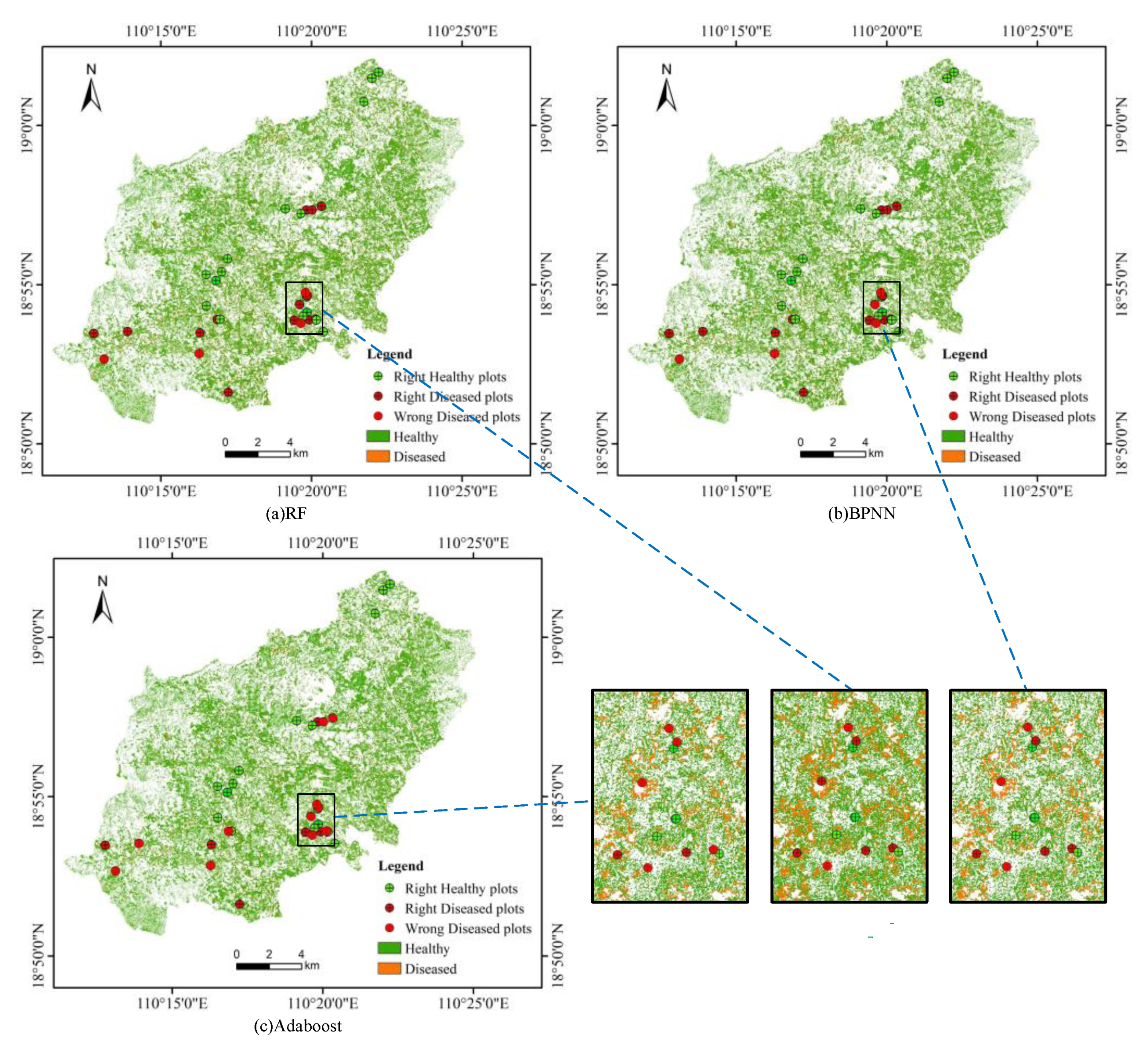
3.2. Recognizition Model Building and Verification

The feature variables Green, Blue, Red, PSRI and EVI selected via CA and independent sample t-tests were then input into the BPNN, AdaBoost and RF algorithms to construct three double-classification monitoring models for areca yellow leaf disease. The survey data collected in the field was used to verify the model results. Accuracy evaluation of the areca yellow leaf disease monitoring model constructed based on all feature variables and the highly correlated and significant different feature variables Green, Blue, Red, PSRI, EVI, NPCI, RVI, OSAVI, SAVI and MSAVI was compared with the above model.

Table 4. Verification results of the three monitoring models based on feature variables optimization.

Model	Sample	Evaluation Index
		Health	Disease	Sum	Omission (%)	Commission (%)	OA (%)	Kappa
RF	Health	17	4	21	0.00	19.05	88.24	0.765
	Disease	0	13	13	23.53	0.00
	Sum	17	17	34
BPNN	Health	17	5	22	0.00	22.73	85.29	0.706
	Disease	0	12	12	29.41	0.00
	Sum	17	17	34
AdaBoost	Health	17	11	28	0.00	39.29	67.65	0.353
	Disease	0	6	6	64.71	0.00
	Sum	17	17	34

,

Table 5. Verification results of the three monitoring models based on highly correlated and significant different feature variables.

Model	Sample	Evaluation Index
		Health	Disease	Sum	Omission (%)	Commission (%)	OA (%)	Kappa
RF	Health	17	3	20	0.00	15.00	91.18	0.824
	Disease	0	14	14	17.65	0.00
	Sum	17	17	34
BPNN	Health	15	2	17	11.76	11.76	88.24	0.778
	Disease	2	15	12	11.76	11.76
	Sum	17	17	34
AdaBoost	Health	17	10	27	0.00	37.04	73.53	0.412
	Disease	0	7	6	58.82	0.00
	Sum	17	17	34

and

Table 6. Verification results of the three monitoring models based on all feature variables.

Model	Sample	Evaluation Index
		Health	Disease	Sum	Omission (%)	Commission (%)	OA (%)	Kappa
RF	Health	15	4	19	11.76	21.05	82.35	0.647
	Disease	2	13	15	23.53	13.33
	Sum	17	17	34
BPNN	Health	15	9	24	11.76	37.50	68.65	0.353
	Disease	2	8	10	52.94	20.00
	Sum	17	17	34
AdaBoost	Health	17	12	28	0.00	42.86	64.71	0.294
	Disease	0	5	6	70.59	0.00
	Sum	17	17	34

reports the omission, commission, overall accuracy and Kappa coefficient of the three areca yellow leaf disease monitoring models based on feature variables optimization, highly correlated and significant different feature variables and all feature variables, respectively.

In Table 4, the overall accuracy of the RF, BPNN and AdaBoost monitoring models are 88.24%, 85.29%, and 67.65% based on feature variables optimization, with the RF model accuracy surpassing the BPNN and AdaBoost models by 2.95% and 20.59%, respectively. The misclassification and omission errors reveal that RF, BPNN and AdaBoost did not omit any healthy samples, nor did they misclassify diseased samples. However, the three models exhibit different degrees of error in terms of the omission of disease samples and the misclassification of healthy samples, with the RF model associated with the lowest corresponding errors (23.53% and 19.05%, respectively). The AdaBoost model exhibits the greatest omission of disease samples and misclassification of healthy samples at 64.71% and 39.29%, respectively. Furthermore, the Kappa coefficient of the RF model is 0.765, which is 0.059 and 0.412 higher than the values of the BPNN and AdaBoost models, respectively. Thus, the RF model demonstrating the highest overall accuracy and Kappa coefficient, and achieving the highest recognition accuracy.

Comparison with Table 5 and Table 6, the accuracy evaluation of the three areca yellow leaf disease monitoring models based on highly correlated and significant different feature variables were higher than that based on all feature variables. In addition, the accuracy evaluation of the three areca yellow leaf disease monitoring models based on feature variables optimization were also higher than that based on all feature variables.

Thus, the areca yellow leaf disease monitoring models established by highly correlated variables has better performance. In addition, the model built by feature variables optimization through the CA and independent t-testing also has good superiority.

3.3. Areca Yellow Leaf Disease Mapping

The RF, BPNN and AdaBoost based models with the five feature variables (Green, Blue, Red, PSRI and EVI) as input were used to identify areca yellow leaf disease. Figure 3 presents the spatial distribution map of disease severity from the three models. The RF determined distribution map based (Figure 3a) identifies a small number of the arecanut plants in the study area as diseased, with the diseased arecanut plants generally scattered and in the central, northern, and southeast regions. However, there were still some diseased plants that are misclassified as healthy plants. The diseased plants in the BPNN determined distribution map (Figure 3b) are generally concentrated within the central, southeast and northeast regions, with a sporadic distribution in other regions. Furthermore, many diseased arecanut plants are omitted and some diseased arecanut plants are misclassified as healthy plants. The AdaBoost determined distribution map (Figure 3c) identifies all arecanut plants in the study area as healthy, with very few diseased plants. Clearly, a large number of diseased arecanut plants are omitted and the diseased arecanut plants are misclassified as healthy plants and thus the AdaBoost model thu s has a weak ability to recognize diseased arecanut plants. The classification and recognition performance of the RF model surpasses the other two models for areca yellow leaf disease in the study area. Thus, PlanetScope images have an applicability in studies identification and monitoring of areca yellow leaf disease [37]. In addition, it has a certain prospect in the identification and monitoring of agricultural and forestry diseases and pests in the future [38,39,40].

4. Discussion

The results demonstrates that the RF algorithm exhibited the highest monitoring accuracy of areca yellow leaf disease, followed by the BPNN and AdaBoost algorithms, respectively. The accuracy of disease monitoring models is highly dependent on the modeling process used. Crop disease remote sensing monitoring models that employ individual classifiers such as SVM and RVM are associated with overfitting problems. In order to avoid this problem, in this paper we selected the ensemble learning algorithm. The ensemble methods can be divided into the Boosting and Bagging algorithms. The Boosting ensemble method selects the most representative AdaBoost algorithm, while Bagging reduces the generalization error by combining several models and selects the most representative Random Forest (RF) algorithm. RF exhibits strong noise tolerance, is capable of handling high-dimensional data, and is also less prone to over-fitting. The RF algorithm is less prone to over-fitting and has a stronger noise tolerance than the BPNN and AdaBoost algorithms, yet its cumbersome parameters and features that take more value divisions tend to have a greater impact on the accuracy of RF. This consequently effects the accuracy of the model. In future research, we will try our best to use disease data for many years and combine multi-source data to find a simpler and more effective feature selection method to screen the input variables of the model, and choose a better model to achieve accurate monitoring of the severity of the disease. In addition, it has a certain prospect in the identification and monitoring of agricultural and forestry pest and disease in the future.

In the study, the accuracy evaluation of the RF monitoring models based on highly correlated and significant different feature variables surpassing based on all feature variables by 8.83%, with the accuracy evaluation of the RF monitoring models based on feature variables optimization surpassing based on all feature variables by 5.89%. The results of this study indicate that the areca yellow leaf disease monitoring models established by highly correlated variables has better performance, as well as the model built by feature variables optimization through the CA and independent t-testing has good superiority. This is attributed to the fact that as the presence of irrelevant, weakly related, or redundant features in the primary selected features will directly affect the classification accuracy and generalization ability of the model [41]. Feature selection is needed to remove these negative features. Previous studies reveal that the green band is sensitive to plant chlorophyll content [18]; the blue band is sensitive to the reaction between chlorophyll and leaf pigment [18]; the red band is an important indicator of plant vitality [19]; PSRI can monitor the onset of plant senescence and canopy stress [42]; and EVI is sensitive to high biomass areas and has a stronger ability to identify crops compared to NDVI [43,44]. Thus, the Green, Blue, Red, PSRI and EVI feature variables were selected through the CA and independent t-testing. However, CA and independent t-testing are associated with several limitations in feature screening. For example, the CA approach lacks an effective redundancy analysis between features, and redundant features cannot be removed from the feature subset, reducing the learning performance of the classification model [45]. In addition, t-testing only determines the inter-class differences of features, ignoring the connection between features and class labels. The selection of a simpler and more efficient algorithm to optimize the spectral feature variables is reserved for future research.

With the development of artificial intelligence, pattern recognition and machine learning methods will become more prevalent for monitoring and forecasting of crop diseases using remote sensing [46]. At present, there is little research on the monitoring of areca yellow leaf disease. It is necessary to explore the feasibility of large-scale regional remote sensing monitoring of areca yellow leaf disease on PlanetScope images, and clarify the applicability of different remote sensing monitoring methods of areca yellow leaf disease. In this study, the monitoring model constructed only based on spectral features is not sufficient to solve some special situations in complex environments, we can combine with time, location and characteristics of onset of areca yellow leaf disease to determining the possibility of confusing yellow leaf disease with bud/crown rot or with tree senescence. Later, we can combine with the correlation and time-continuous features of areca yellow leaf disease (the meteorological, GIS data) to improve the adaptability of the monitoring model to the growth environment of arecanut, to construct a more accurate monitoring and identification model of areca yellow leaf disease, and eventually to achieve more accurate and efficient monitoring and identification of areca yellow leaf disease in a large area. This study only used one phase PlanetScope images to monitor the spatial distribution of areca yellow leaf disease, and did not consider the effects of drought, nitrogen deficiency and other physiological yellow leaf diseases. How to use multi-temporal with more regional data for in-depth verification analysis is also the follow-up work to be carried out. In the future, according to the physiological features of areca yellow leaf disease in Hainan, we will use multi-temporal images to analyze the incidence of arecanut during different critical periods of arecanut growth, and build a more accurate arecanut growth monitoring and identification model. In addition, the comparative analysis of the monitoring results of areca yellow leaf disease based on different remote sensing data sources, even sub-meter high-resolution remote sensing images, is also a follow-up work to be carried out. Hainan is characterized by a cloudy and rainy climate. Satellite remote sensing is easily obscured by clouds and fog, often unable to obtain clear images, and the period of obtaining images is relatively long. Unmanned aerial vehicle (UAV) remote sensing can make up for the shortcomings of satellite remote sensing, and the obtained images also have higher resolution; therefore, coordinated satellite and UAV remote sensing for yellow leaf disease monitoring is also a future development trend.

5. Conclusions

Compared with field crops such as wheat, the remote sensing monitoring of areca yellow leaf disease is limited in some regions (i.e., the tropical and subtropical regions) with fragmented plots and cloudy and rainy weather. This study is based on PlanetScope images to carry out remote sensing monitoring of areca yellow leaf disease for a large-scale regional. Results demonstrate the RF model exhibits the highest overall recognition accuracy for areca yellow leaf disease (88.24%), 2.95% and 20.59% higher than the BPNN and AdaBoost models, respectively. The RF-based spatial distribution map achieves the higher recognition accuracy. In addition, compared with the BPNN and AdaBoost algorithms, it is more suitable for the identification and monitoring of areca yellow leaf disease. The research results provide a reference for the regional large-scale monitoring and prevention of crop diseases and pests.

References

1. Office of the Development of South Subtropical Crops, Ministry of Agriculture. Production of Tropical, Southern and Subtropical Crops of the Ministry of Agriculture, 2007th ed.; South Subtropical Crops Development Office, Ministry of Agriculture: Beijing, China, 2008; pp. 343–356.
2. Che, H.; Cao, X.; Xuan, Z.; Luo, D. Betel nut yellowing disease “should be prevented” or “cured”. China Trop. Agric. 2018, 5, 46–48. [Google Scholar]
3. Manimekalai, R.; Sathish Kumar, R.; Soumya, V.P.; Thomas, G.V. Molecular Detection of Phytoplasma Associated with Yellow Leaf Disease in Areca Palms (Areca catechu) in India. Plant Dis. 2010, 94, 1376. [Google Scholar] [CrossRef]
4. Che, H.; Cao, X.; Luo, D. Research and Demonstration Application of Diagnosis and Rapid Pathogen Detection Technology of Areca Yellow Leaf Disease in Hainan. In Proceedings of the China Plant Protection Society 2019 Annual Conference, Guiyang, China, 23–25 October 2019. [Google Scholar]
5. Zhang, J.; Li, J.; Yang, G.; Yang, G.; Huang, W.; Luo, J.; Wang, J. Monitoring of Winter Wheat Stripe Rust Based on the Spectral Knowledge Base for TM Images. Spectrosc. Spectr. Anal. 2010, 30, 1579–1585. [Google Scholar]
6. Franke, J.; Menz, G. Multi-temporal Wheat Disease Detection by Multi-spectral Remote Sensing. Precis. Agric. 2007, 8, 161–172. [Google Scholar] [CrossRef]
7. Tang, C.; Huang, W.; Luo, J.; Liang, D.; Zhao, J.; Huang, L. Forecasting Wheat Aphid with Remote Sensing Based on Relevance Vector Machine. Trans. Chin. Soc. Agric. Eng. 2015, 31, 201–207. [Google Scholar]
8. Ma, H.; Huang, W.; Jing, Y.; Dong, Y.; Zhang, J.; Nie, C.; Tang, C.; Zhao, J.; Huang, L. Remote Sensing Monitoring of Wheat Powdery Mildew Based on AdaBoost Model Combining mRMR Algorithm. Trans. Chin. Soc. Agric. Eng. 2017, 33, 162–169. [Google Scholar]
9. Yuan, L.; Pu, R.; Zhang, J.; Wang, J.; Yang, H. Using high spatial resolution satellite imagery for mapping powdery mildew at a regional scale. Precis. Agric. 2016, 17, 332–348. [Google Scholar] [CrossRef]
10. Gašparović, M.; Medak, D.; Pilaš, I.; Jurjević, L.; Balenović, I. Fusion of sentinel-2 and Planetscope imagery for vegetation detection and monitoring. Int. Arch. Photogramm. Remote Sens. Spat. Inf. Sci. 2018, XLII-1, 155–160. [Google Scholar] [CrossRef] [Green Version]
11. Jin, Y.; Guo, J.; Ye, H.; Zhao, J.; Huang, W.; Cui, B. Extraction of Arecanut Planting Distribution Based on the Feature Space Optimization of PlanetScope Imagery. Agriculture 2021, 11, 371. [Google Scholar] [CrossRef]
12. Gasparovic, M.; Dobrinic, D.; Medak, D. Urban Vegetation Detection Based on The Land- Cover Classification of PlanetScope, RapidEye and WorldView-2 Satellite Imagery. In Proceedings of the 2018 18th International Multidisciplinary Scientific GeoConference SGEM2018 Work, Albena, Bulgaria, 2–8 July 2018; International Multidisciplinary Scientific GeoConference-SGEM: Sofia, Bulgaria, 2018; Volume 7, pp. 1314–2704. [Google Scholar] [CrossRef] [Green Version]
13. Szabó, L.; Abriha, D.; Phinzi, K.; Szabó, S. Urban vegetation classification with high-resolution PlanetScope and SkySat multispectral imagery. Landsc. Amp. Environ. 2021, 15, 66–75. [Google Scholar] [CrossRef]
14. Hainan Provincial Bureau of Statistics. Hainan Statistical Yearbook, 2019th ed.; China Statistical Publishing House: Beijing, China, 2020; pp. 217–266.
15. Yang, C.; Zhan, Q.; Zhou, Y.; Zhang, Y. Investigation on the Condition of Areca yellow leaf disease in the South of Wanning. China Pharm. 2018, 27, 70–71. (In Chinese) [Google Scholar]
16. Wang, F.; Yao, F.; Chen, Y.; Chen, C. Monitoring Study on the Influence of Hainan International Tourism Island Construction to the Mangrove Forest Based on RS and GIS. Adv. Mat. Res. 2011, 1198, 33–38. [Google Scholar] [CrossRef]
17. Planet Team. Planet Application Program Interface: In Space for Life on Earth; Planet Team: San Francisco, CA, USA, 2018. [Google Scholar]
18. Huang, Z.; Cao, C.; Chen, W.; Xu, M.; Dang, Y.; Singh, R.P.; Bashir, B.; Xie, B.; Lin, X. Remote sensing monitoring of vegetation dynamic changes after fire in the Greater Hinggan Mountain Area: The algorithm and application for eliminating phenological impacts. Remote Sens. 2020, 12, 156. [Google Scholar] [CrossRef] [Green Version]
19. Zeng, C.; Binding, C. The Effect of Mineral Sediments on Satellite Chlorophyll-a Retrievals from Line-Height Algorithms Using Red and Near-Infrared Bands. Remote Sens. 2019, 11, 2036. [Google Scholar] [CrossRef] [Green Version]
20. Huete, A.R.; Jackson, R.D. Suitability of spectral indices for evaluating vegetation characteristics on arid rangelands. Remote Sens. Environ. 1987, 23, 213–232. [Google Scholar] [CrossRef]
21. Jordan, C.F. Derivation of leaf area index from quality of light on the forest floor. Ecology 1969, 50, 663–666. [Google Scholar] [CrossRef]
22. Goel, N.S.; Qin, W. Influences of canopy architecture on relationships between various vegetation indices and LAI and Fpar: A computer simulation. Remote Sens. Rev. 1994, 10, 309–347. [Google Scholar] [CrossRef]
23. Penuelas, J.; Gamon, J.A.; Fredeen, A.L.; Merino, J.; Field, C.B. Reflectance indices associated with physiological changes in nitrogen-and water-limited sunflower leaves. Remote Sens. Environ. 1994, 48, 135–146. [Google Scholar] [CrossRef]
24. Chen, S.F.; Goodman, J. An empirical study of smoothing techniques for language modeling. ACL 1999, 13, 310–318. [Google Scholar] [CrossRef] [Green Version]
25. Merzlyak, M.N.; Gitelson, A.A.; Chivkunova, O.B.; Rakitin, V.Y. Non-destructive optical detection of leaf senescence and fruit ripening. Physiol. Plantarum. 1999, 106, 135–141. [Google Scholar] [CrossRef] [Green Version]
26. Huemmrich, K.F.; Black, T.A.; Jarvis, P.G.; McCaughey, J.H.; Hall, F.G. High temporal resolution NDVI phenology from micrometeorological radiation sensors. JGR Earth Surf. 1999, 104, 27935–27944. [Google Scholar] [CrossRef]
27. Huete, A.R. A soil-adjusted vegetation index (SAVI). Remote Sens. Environ. 1988, 25, 295–309. [Google Scholar] [CrossRef]
28. Rondeaux, G.; Steven, M.; Baret, F. Optimization of Soil-Adjusted Vegetation Indices. Remote Sens. Environ. 1996, 55, 95–107. [Google Scholar] [CrossRef]
29. Zhao, Y.; Potgieter, A.B.; Zhang, M.; Wu, B.; Hammer, G.L. Predicting Wheat Yield at the Field Scale by Combining High-Resolution Sentinel-2 Satellite Imagery and Crop Modelling. Remote Sens. 2020, 12, 1024. [Google Scholar] [CrossRef] [Green Version]
30. Ren, S.; Chen, X.; An, S. Assessing plant senescence reflectance index-retrieved vegetation phenology and its spatiotemporal response to climate change in the Inner Mongolian Grassland. Int. J. Biometeorol. 2017, 61, 601–612. [Google Scholar] [CrossRef] [PubMed]
31. Kwok, S.W.; Carter, C. Multiple Decision Trees. Mach. Intell. 2013, 9, 327–335. [Google Scholar] [CrossRef]
32. Santana, F.B.; Neto, W.B.; Poppi, R.J. Random forest as one-class classifier and infrared spectroscopy for food adulteration detection. Food Chem. 2019, 293, 323–332. [Google Scholar] [CrossRef]
33. Belgiu, M.; Drăguţ, L. Random forest in remote sensing: A review of applications and future directions. ISPRS J. Photogramm. Remote Sens. 2016, 114, 24–31. [Google Scholar] [CrossRef]
34. Wang, S.; Zhang, N.; Wu, L.; Wang, Y. Wind Speed Forecasting Based on the Hybrid Ensemble Empirical Mode Decomposition and GA-BP Neural Network Method. Renew. Energy 2016, 94, 629–636. [Google Scholar] [CrossRef]
35. Schapire, R.E.; Freund, Y.; Bartlett, P.; Lee, W.S. Boosting the margin: A new explanation for the effectiveness of voting methods. Ann. Stat. 1998, 26, 1651–1686. [Google Scholar] [CrossRef]
36. Guo, L.; Xi, X.; Yang, W.; Liang, L. Monitoring Land Use/Cover Change Using Remotely Sensed Data in Guangzhou of China. Sustainability 2021, 13, 2944. [Google Scholar] [CrossRef]
37. Shi, Y.; Huang, W.; Ye, H.; Ruan, C.; Xing, N.; Geng, Y.; Dong, Y.; Peng, D. Partial Least Square Discriminant Analysis Based on Normalized Two-Stage Vegetation Indices for Mapping Damage from Rice Diseases Using PlanetScope Datasets. Sensors 2018, 18, 1901. [Google Scholar] [CrossRef] [PubMed] [Green Version]
38. Manivasagam, V.S.; Sadeh, Y.; Kaplan, G.; Bonfil, D.J.; Rozenstein, O. Studying the Feasibility of Assimilating Sentinel-2 and PlanetScope Imagery into the SAFY Crop Model to Predict Within-Field Wheat Yield. Remote Sens. 2021, 13, 2395. [Google Scholar] [CrossRef]
39. Zhao, J.; Jin, Y.; Ye, H.; Huang, W.; Dong, Y.; Fan, L.; Ma, H.; Jiang, J. Remote sensing monitoring of areca yellow leaf disease based on UAV multi-spectral images. Trans. Chin. Soc. Agric. Eng. 2020, 36, 54–61. [Google Scholar]
40. Pickering, J.; Tyukavina, A.; Khan, A.; Potapov, P.; Adusei, B.; Hansen, M.C.; Lima, A. Using Multi-Resolution Satellite Data to Quantify Land Dynamics: Applications of PlanetScope Imagery for Cropland and Tree-Cover Loss Area Estimation. Remote Sens. 2021, 13, 2191. [Google Scholar] [CrossRef]
41. Sun, Z.; Bebis, G.; Miller, R. Object detection using feature subset selection. Pattern Recognit 2004, 37, 2165–2176. [Google Scholar] [CrossRef]
42. Gu, Z.; Ju, W.; Liu, Y.; Li, D.; Fan, W. Forest Leaf Area Index Estimated from Tonal and Spatial Indicators Based on IKONOS_2 Imagery. IJRSA 2013, 3, 175–184. [Google Scholar] [CrossRef]
43. Hinojo-Hinojo, C.; Goulden, M.L. Plant Traits Help Explain the Tight Relationship between Vegetation Indices and Gross Primary Production. Remote Sens. 2020, 12, 1405. [Google Scholar] [CrossRef]
44. Villamuelas, M.; Fernández, N.; Albanell, E.; Gálvez-Cerón, A.; Bartolomé, J.; Mentaberre, G.; López-Olvera, J.R.; Fernández-Aguilar, X.; Colom-Cadena, A.; López-Martín, J.M.; et al. The Enhanced Vegetation Index (EVI) as a proxy for diet quality and composition in a mountain ungulate. Ecol. Indic. 2016, 61, 658–666. [Google Scholar] [CrossRef]
45. Dash, M.; Liu, H. Feature selection for classification. Intell. Data Anal. 1997, 1, 131–156. [Google Scholar] [CrossRef]
46. Lu, J.; Sun, L.; Huang, W. Research progress in monitoring and forecasting of crop pests and diseases by remote sensing. Remote Sens. Technol. Appl. 2019, 34, 21–32. [Google Scholar]
Figure 1. Location of the study area with the distribution of survey sample sites, and coordinate system using WGS84, (a) Side view and vertical view of healthy arecanut; (b) Side view and vertical view of diseased arecanut.
Agronomy 12 00014 g001
Figure 2. Box-scatterplots of reflectance of healthy arecanut and diseased arecanut.
Agronomy 12 00014 g002
Figure 3. Distribution map and detail view of areca yellow leaf disease severity determined from Planet imagery via (a) RF, (b) BPNN and (c) AdaBoost.
Agronomy 12 00014 g003