UAV- and Random-Forest-AdaBoost (RFA)-Based Estimation of Rice Plant Traits

Abstract

Rapid, accurate and inexpensive methods are required to analyze plant traits throughout all crop growth stages for plant phenotyping. Few studies have comprehensively evaluated plant traits from multispectral cameras onboard UAV platforms. Additionally, machine learning algorithms tend to over- or underfit data and limited attention has been paid to optimizing their performance through an ensemble learning approach. This study aims to (1) comprehensively evaluate twelve rice plant traits estimated from aerial unmanned vehicle (UAV)-based multispectral images and (2) introduce Random Forest AdaBoost (RFA) algorithms as an optimization approach for estimating plant traits. The approach was tested based on a farmer’s field in Terengganu, Malaysia, for the off-season from February to June 2018, involving five rice cultivars and three nitrogen (N) rates. Four bands, thirteen indices and Random Forest-AdaBoost (RFA) regression models were evaluated against the twelve plant traits according to the growth stages. Among the plant traits, plant height, green leaf and storage organ biomass, and foliar nitrogen (N) content were estimated well, with a coefficient of determination (R²) above 0.80. In comparing the bands and indices, red, Normalized Difference Vegetation Index (NDVI), Ratio Vegetation Index (RVI), Red-Edge Wide Dynamic Range Vegetation Index (REWDRVI) and Red-Edge Soil Adjusted Vegetation Index (RESAVI) were remarkable in estimating all plant traits at tillering, booting and milking stages with R² values ranging from 0.80–0.99 and root mean square error (RMSE) values ranging from 0.04–0.22. Milking was found to be the best growth stage to conduct estimations of plant traits. In summary, our findings demonstrate that an ensemble learning approach can improve the accuracy as well as reduce under/overfitting in plant phenotyping algorithms.

1. Introduction

In recent years, remote sensing platforms, especially aerial unmanned vehicle (UAV) and image processing methods, have been intensively explored as a preliminary step to plant phenotyping [1,2,3,4]. The ultimate advantage of UAV for plant phenotyping lies upon its ability to obtain better spatial, spectral and temporal resolutions compared to satellite data. UAV-crop phenotyping has been considered as a valuable tool given its capability to provide a solution to determining genomic-enable enhancements in a precise, efficient, flexible, rapid and non-destructive manner [5].

Simultaneously, many recent studies [6,7,8,9,10,11,12,13,14,15,16,17] have demonstrated the capability of UAV based sensors to estimate common rice agronomics traits such as leaf or/and plant N content, the biomass of separate crop organs, yield components and other physiological responses that are useful for phenotyping studies. These traits are commonly used to evaluate the effects of fertilizers, irrigation management and weather on the rice crop growth development, either through field experiments or crop modelling [18,19,20] since they are direct indicators of rice growth and yield performance. Generally, the results from past studies have illustrated that plant traits such as leaf or/and plant N content, biomass and yield could be inferred using various indices at different rice growing stages with good accuracy [6,7,8,9,10,11,12]. Fewer studies have been conducted for the rice leaf area index (LAI), plant height (PH), plant density and chlorophyll content [6,8,13,14,15,16,17].

In the latest exploration, researchers have attempted to implement a nonparametric regression model through machine learning (ML) algorithms in their estimation models to increase the accuracy. Among the machine learning algorithms, RF is one of many that has been rigorously explored in agriculture, with various degrees of success. The superior performance of RF was reported by Wang et al. [21], Ndikumana et al. [22], Zha et al. [23] and Liang et al. [24]. Wang et al. [21] demonstrated that the bagged RF performance in the estimation of rice LAI was better than neural network and PLS but comparable to support vector regression. Ndikumana et al. [22], in a study utilizing satellite data to estimate rice PH and dry biomass, found that RF yielded the best performance in comparison to other ML algorithms tested, such as SVR. Zha et al. [23], in studying multiple rice traits at two growth stages using UAV images, found that RF algorithms outperformed SVR and ANN. In their leaf N study, Liang et al. [24] reported that RF regression was better than the least square SVR and curve fitting models. On other hand, Sun et al. [25], Yuan et al. [26] and Apolo-Apolo et al. [27] found that the performance of RF algorithms was poorer than other machine learning algorithms, such as back-propagation neural network (BPNN) (leaf N of rice), SVM (LAI of soybean) and ANN (LAI of wheat). Sun et al. [25] reported that for all the sensors tested in their study, RF produced better results compared to BPNN and SVM. Yuan et al. [26] found that the RF performed poorly in estimating the LAI of soybean at single growth stages, although the models for the whole growth period depicted contradicting results. Authors such as Liang et al. [24] have attributed the better performance of the RF algorithm to the ability of the algorithm to improve the overall prediction accuracy through combinations of different independent predictors that are possibly misclassified individually; nonetheless it still suffered from underfitting problems—a concern that has been emphasized by Jeong et al. [28], Wang et al. [21] and Zha et al. [23].

Meanwhile, the recent exploration of adaptive boosting (AdaBoost) algorithms in agricultural studies is still limited. In a rice yield prediction study, Mishra et al. [29] reported that strong learners such as AdaBoost regressor increased the R² values and produced few errors when integrated into weak learners such as linear regression (LR) and SVR. Nevertheless, Sun et al. [30], in a study to predict the end-of-season potato tuber yield and tuber set using in-season UAV-based hyperspectral images and multiple MLs, portrayed that AdaBoost performed poorly compared to the rest of the tested algorithms, with the best estimation being obtained through ridge regression. However, El Bilali and Taleb [31], in assessing several MLs such as ANN, MLR, RF, SVR and Adaboost for predicting irrigation water quality, reported that the Adaboost algorithm performed better than DT and was comparable to RF, but not ANN and MLR.

While many researchers have demonstrated the capability of UAV for crop phenotyping and estimating rice plant traits, the majority of conducted studies have focused on a single or four traits at most [6]. However, in actual breeding studies, breeders may find it interesting to simultaneously phenotype many agronomic traits that act as yield components. Currently, there are scant works that have comprehensively evaluated many plant traits from multispectral cameras onboard UAV platforms. Additionally, the existing literature illustrates that traits have often been estimated using various indices at different growth stages, implying the limitation that the indices are commonly growth stage dependent. Other than at tillering and heading stages, the estimation of plant traits has appeared to be challenging due to secondary factors such as the soil background and panicle. Furthermore, these machine learning-related agriculture studies show that many individual machine learning algorithms, including the smart learners such as RF, still tend to over or underfit data when they are dealing with limited or complicated data. Most of these studies have compared the performance of existing machine learning algorithms, while limited attention has been paid to optimizing their performances through an ensemble learning approach, whereby two learners are combined for an optimization of performance [22,25,29,30]. RF is a widely implemented machine learning regressor in agriculture due to its simplicity in comparison to other regressors such as SVR and ANN. However, its performance when coupled to AdaBoost has not been assessed in agricultural studies.

In light of this, this research aims to comprehensively evaluate twelve rice plant traits that could be effectively estimated and predicted from UAV based multispectral images at three growth stages through the best vegetation index (or indices) and to evaluate ensemble RF-AdaBoost algorithms as an optimization approach. This study is the first to test the combination of RF and AdaBoost machine learning algorithms in terms of their accuracy in estimating rice plant traits.

2. Materials and Methods

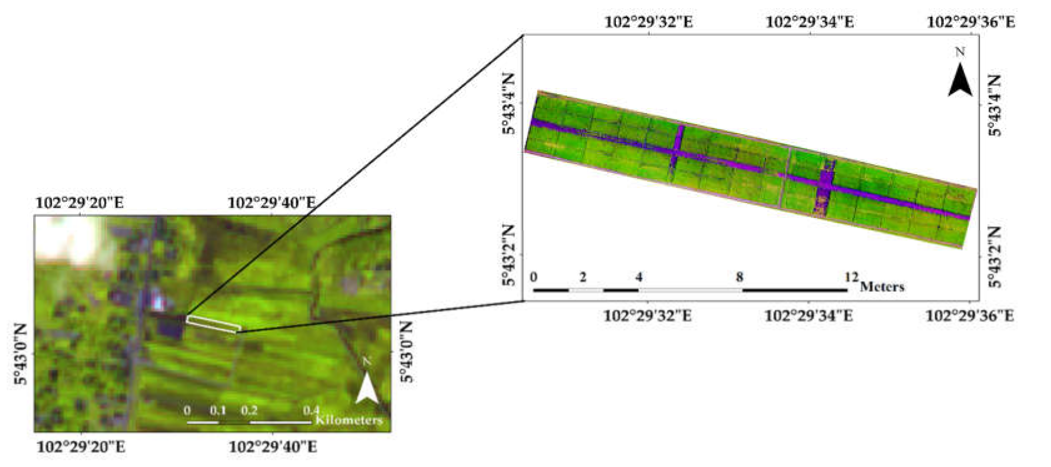
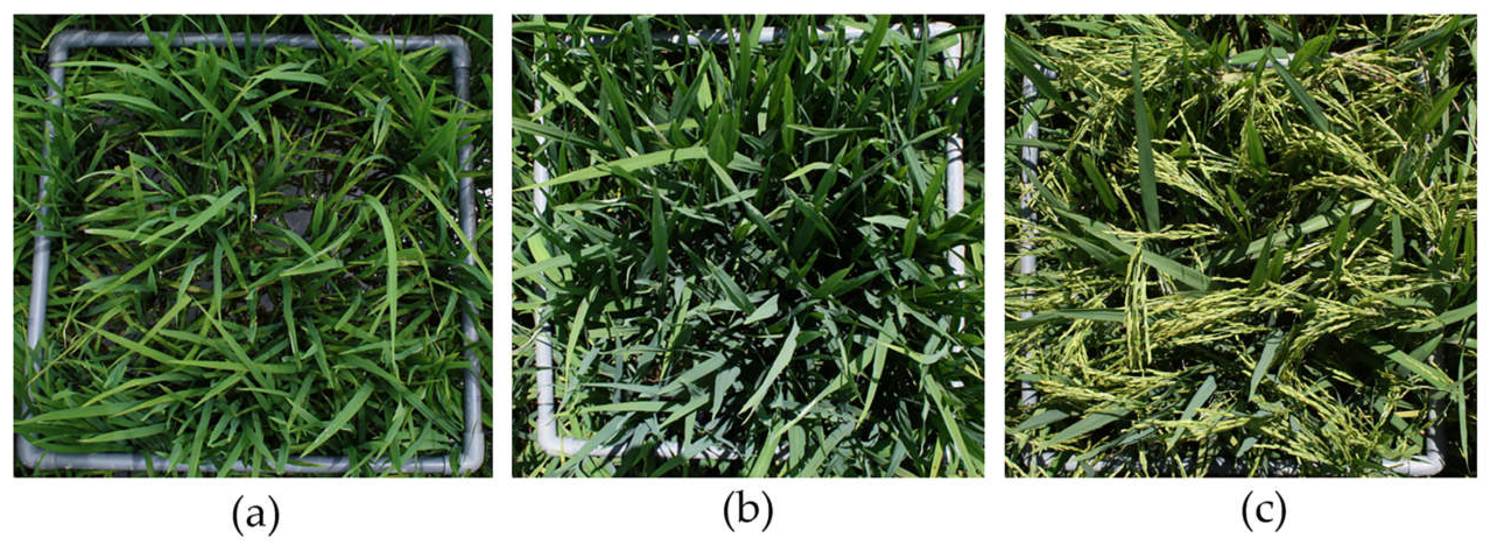
2.1. Experimental Sites and Design

This study was conducted at a farmer’s field in IADA KETARA, Lubuk Kawah, Jerteh Terengganu (5°43′4″ N, 102°29′33″ E (World Geodetic System (WGS) 1984)) (Figure 1) during the off-season from February to June 2018. The experimental design was a split plot in a randomized complete block design (RCBD), with the nitrogen (N) rates as the main effect and cultivar as the sub-effect. Five cultivars, MR269, MR220 CL2, MR219, MR297, and UPUTRA, were chosen based on their frequency of usage in Malaysian granaries (MR220 CL2 at about 50%, MR219 at 24%, MR263 at 13%, MR220 at 5%, MR269 at 3% and other cultivars at 5% [32], while UPUTRA is the most recent cultivar). They were broadcasted in each N plot in 60 experimental units of 11 m × 5 m. All the subplots were seeded between 17 to 20 February 2018. Tilling prior to the seed broadcast was conducted manually to ensure the safety of the plastic bunds separating the main N plots, hence, the seeding days were conducted over several days. N fertilizer rates were applied as follows: 76, 109, and 142 kg ha⁻¹, and henceforth, will be referred to as N1, N2, and N3, respectively, and these were replicated in four blocks. The 109 kg ha⁻¹ rate is the best farmers’ practice rate, and 30% of the N input was reduced or added to formulate N1 and N3, respectively, in order to induce differences in plant trait characteristics. Application of N fertilizer was made in three split applications as practiced by the best farmers in the granary areas according to development of the vegetative phase: 39% at the germination stage (18 days after seeding (DAS)), 42% at the end of effective tillering (39 DAS), and 19% at the panicle initiation stage (55 DAS). Other nutrients were applied as standard agronomic practices. The bunds were constructed and covered with polyethylene polybags to separate the cultivars and reduce the risk of nitrogen seepage through the bunds. The water was kept constantly flooded between 5 to 10 cm until 15 days before harvesting.

2.2. Field Data Collection

2.2.1. Ground Data

Plant trait data was measured at four sampling campaigns: 34 to 37 DAS, 62 to 65 DAS, 83 to 86 DAS and 104 to 105 DAS. The crop growth stage at these sampling campaigns according to the principal growth stage of Biologische Bundesanstalt, Bundessortenamt and Chemical (BBCH)-scale was tillering, booting, milking, and harvesting, respectively [33]. The first three sampling campaigns were specifically chosen to represent vegetative, reproductive and maturing phases. Two sets of samples were taken from each experimental unit, resulting in a total of 120 samples per campaign and the sampling was limited to 30 samples per day. The first seeded plots were sampled first to accommodate the difference in the seeding dates. Plant traits collected were the number of plants (NOP) (unitless), maximum plant height (PH) (m), chlorophyll content (SPAD) (SPAD units), leaf color chart (LCC) (unitless), leaf area index (LAI) (unitless), green leaf (GL) biomass (g quadrant⁻¹), dead leaf (DL) biomass (g quadrant⁻¹), stem (STEM) biomass (g quadrant⁻¹), storage organ (SO) biomass (g quadrant⁻¹), total (TOTAL) biomass (g quadrant⁻¹), panicle yield (YIELD) biomass (g quadrant⁻¹) and foliar nitrogen content (NC) (%). Two quadrants of 0.5 m × 0.5 m were placed randomly in each experimental plot and their coordinate values were recorded using a Trimble R8 RTK with a maximum precision of up to 8 mm and 15 mm for vertical and horizontal accuracy, respectively. The UTM WGS 1984 zone 48 N was set as the coordinate reference system. The number of rice plants per quadrant was counted. Afterwards, above ground plant biomass was uprooted manually for each quadrant using a sickle. The maximum plant height for ten randomly selected plants was measured for each set of samples using a standard measuring tape, and then averaged. Further, SPAD meter readings were measured from the first ten fully expanded uppermost leaves of the same selected plants by using a Minolta SPAD 502 Chlorophyll Meter (Minolta Corp., Osaka, Japan). The readings were then averaged. Next, the level of leaf greenness from the previously selected leaf samples was measured based on four panel series from yellow–green to dark green as provided by the standard leaf color chart [34] and also averaged. However, for panicle yield, four quadrants were randomly sampled a day prior to the harvesting day in each experimental plot and averaged. Later, all the samples were packed and stored in iced coolers and transported to Universiti Putra Malaysia (UPM) (2.9998° N, 101.7121° E). Upon arrival, the plant samples were detached and classified according to green leaf blades, dead leaf blades, stem, and storage organs (if applicable). Then, the leaves were cleaned to remove contaminants such as water and soil and immediately scanned for leaf area using the Li-Cor 3100 C (Li-cor Inc., Lincoln, NE, USA). The leaf area index (LAI) was calculated using the Equation (1) as follows:

$$LAI=LA/Q$$

(1)

LA is the leaf area (cm²) and Q is the area of quadrant (cm²).

Then, all fragments of the samples were dried until achieving a constant weight. Further, the plant organ biomass was weighted using an analytical balance. For foliar N content analysis, green leaves were pulverized using the Cross Beater Mill SK 100 grinder until they could pass through a 1 mm sieve. Wet digestion, using sulfuric acid (H₂ SO₄) and hydrogen peroxide (H₂ O₂), was conducted to analyze the N content [35]. The digests were sent to the laboratory to determine the total N content (%) using the LACHAT quikChem FIA + 8000 series autoanalyzer (Danaher Corp., Loveland, CO, USA).

2.2.2. Spectral Data

Multispectral images were acquired simultaneously with the ground data collected at two hours before and after local solar noon. Four vertices coordinates were used to set up the flight path from the field. The flying altitude was set up approximately 50 m above the local terrain and resulted in a ground sample distance (GSD) of 3 cm. Side and front laps were approximately 75%. A MicaSense Red-Edge multispectral camera with a gimbal was mounted on a DJI Quadcopter drone. The sensor provides images in five narrow bands (455 to 880 nm) via five separate imaging sensors that operate nearly simultaneously. The gimbal was used to keep the vibration to a minimum and to ensure the camera point straight to the nadir. The sensor was calibrated using MicaSense Calibrated Reflectance Panel (CRP) model RP02 before and after each flight take-off or landing.

2.3. Image Pre-Processing

The Pix4 DMapper Pro (version 4.0, Pix4 D Lausanne, Switzerland) was used to align the five separated images. All geolocation and camera model information was loaded automatically from metadata to prevent band to band misalignment. A Ag Multispectral method was selected as the processing template to generate a reflectance map, index map and application map. In short, there were three image pre-processing stages as follows: (i) initial processing, (ii) point cloud and mesh (iii) Digital Surface Model (DSM), orthomosaic and index. In general, the first step was set following a default. Subsequently, the dense point cloud was generated using three parameters as follows: image scale: ½, point density: optimal, and minimum number of matches: 3. Then, for the third step, radiometric correction was set up, whereby each band was calibrated with known reflectance values from the CRP. The sequence of bands in Pix4 D was as follows: blue, green, red, near infrared and red-edge. Then, all bands were stored in GeoTiff format.

2.4. Data Processing

2.4.1. Raw and Indices Calculation and Extraction

Next, all the five bands from each sampling date were composited to a single raster using the ArcGIS software resulting in three single rasters. The bands were rearranged as follows: band 1 for blue, band 2 for green, band 3 for red, band 4 for red-edge and band 5 for NIR. For each single raster, areas of interest, i.e., the location of the 0.5 m × 0.5 m sampling quadrant were located based on their coordinates and their pixel values were extracted for each band. Extracted pixels were further divided into three different groups of raw bands, a combination of visible and NIR indices as well as a combination of red-edge and NIR indices. The raw bands and indices were tested are tabulated as in

Table 1. Summary of raw bands and vegetation indices.

Index	Equation	Reference
Raw bands
Blue
Green
Red
Red-Edge
NIR
Visible-NIR indices
Normalized Difference Vegetation Index (NDVI)	$\left(NIR-Red\right)/\left(NIR+Red\right)$	Rouse et al. [41]
Green Normalized Difference Vegetation Index (GNDVI)	$\left(NIR-Green\right)/\left(NIR+Green\right)$	Gitelson et al. [42]
Ratio Vegetative Index (RVI)	$NIR/Red$	Pearson and Miller [43]
Difference Vegetation Index (DVI)	$NIR-Red$	Birth and McVey [44]
Renormalized Difference Vegetation Index (RDVI)	$\left(NIR-Red\right)/\sqrt{\left(NIR+Red\right)}$	Roujean and Breon [45]
Red-edge-NIR indices
Normalized Difference Red-Edge Index (NDRE)	$\left(NIR-Red Edge\right)/\left(NIR+Red Edge\right)$	Barnes et al. [46]
Red-Edge Ratio Vegetation Index (RERVI)	$NIR/Red-Edge$	Gitelson et al. [47]
Red-Edge Difference Vegetation Index (REDVI)	$NIR-Red-Edge$	Cao et al. [36]
Red-Edge Renormalized Different Vegetation Index (RERDVI)	$\left(NIR-Red Edge\right)/\sqrt{\left(NIR+Red Edge\right)}$	Cao et al. [36]
Red-Edge Wide Dynamic Range Vegetation Index (REWDRVI)	$\left(0.12\times NIR-Red Edge\right)/\left(0.12\times NIR+Red Edge\right)$	Cao et al. [36]
Red-Edge Soil Adjusted Vegetation Index (RESAVI)	$1.5\times \left(\left(NIR-Red Edge\right)/\left(NIR+Red Edge+0.5\right)\right)$	Cao et al. [36]
Red-Edge Optimized Soil Adjusted Vegetation Index (REOSAVI)	$\left(1+0.16\right)\times \left(\left(NIR-Red Edge\right)/\left(NIR+Red Edge+0.16\right)\right)$	Cao et al. [36]

. The selected indices are commonly evaluated indices in rice experiments [6,8,9,11,12,36,37,38,39,40] with varying degrees of performance for estimating plant traits.

2.4.2. Machine Learning Algorithm

The Scikit-learn package [48], which is an open-source python module, was implemented to interpret and test the data between three groups of indices and twelve plant traits collected at three crop growth stages. The testing involved individual plant traits collected at individual growth stages as the dependent variable, and individual indices as the independent variable. In total, 595 combinations of plant traits, indices and growth stages were tested. Each ground-collected plant trait was associated with the pixel values from the UAV images according to their date of acquisition, with the exception of the yield. Rather than ‘estimation’ of yield, the yield values were paired with the UAV images taken prior to the harvesting date, and thus, the term ‘prediction’ was used. The variables collected the two quadrants from each plot were then averaged, resulting in 60 data points for each sampling date. Calibration was then set up randomly at 60% for training (n = 36) and 40% for testing (n = 24) [17,49]. In addition, all the data were transformed from 0 to 1 as a pre-processing method to standardize the data.

Random Forest-AdaBoost (RFA) Regressor

In general, random forest (RF) is a collection of regression decision trees, each of which is grown on a separate bootstrap sample derived from the original dataset. Each new bootstrap sample is generated based on a random and redundant sampling. Hence, each of the data points in the dataset may be used multiple times in different single trees, but at the same time, certain input data might not be selected. The error between unused data, which is referred as the out-of-bag (OOB) data, and prediction by the regression tree, is measured using mean squared residual error formulae. Typically, two-thirds of the data are used for the construction of a single tree, while the remainder is used as OOB data. The OOB, or bagging technique, is designed to obtain unbiased estimates of regression tree and hyperparameters used for the construction of each single tree.

To construct each tree, hyperparameters are used to improve the model performance and decrease computational speed. There are five majors tuning hyperparameters for RF which are n_estimator, max_feature, max_depth, min_sample_split and min_sample_leaf.

Table 2. Summary of hyperparameter for Random Forest-Adaboost regression model.

Parameter	Description	Randomize Search Value
n_estimators	The number of regression trees in the forest. The higher the n_estimator parameter, the larger is the number of trees created.	10–200
max_features	The maximum number of features for splitting the node.	Auto, sqrt, log2
max_depth	The maximum depth of each regression tree.	10–200
min_samples_split	The minimum number of samples for splitting an internal node.	2–10
min_samples_leaf	The minimum number of samples needed to be at a leaf node.	1–4

lists the hyperparameters, their descriptions and their range values. To optimize these five tuning parameters in order to avoid data overfitting, random search algorithms were employed based on Mao et al. [50]. Random search algorithms are iterations of different numbers of combinations for controlling the performance of data. The other parameters of the RF model were set as default values.

Although RF subtrees grow based on the training dataset through bagging, the average for all single trees is trained via parallel processing, which focuses only on a combination of strong prediction models [51], leading to data bias. Bagging, despite its widespread use in machine learning models to improve overfitting and reduce the variance of the data [52], suffers from the limitations of a small data quantity, data distribution and data quality issues. For example, when the input data are not well distributed or have too much noise, sampling replacement performed during subtree splitting or the data generalization process could cause bias [53] through the repetition use of data in different groups of trees or completely unused data [54]. This collectively causes the RF algorithm to overestimate or underestimate when the observed data are too large or small [55]. Additionally, the RF model is not very sensitive to the tuning parameter for obtaining optimal accuracy of prediction model such as the size of tree that can be in any number.

Given to the limitation of the RF algorithms previously addressed, adaptive boosting, i.e., the AdaBoost regressor was introduced in order to overcome bias estimation by calculating the error and weighting the data to enhance the prediction [29]. The AdaBoost algorithm is similar to the RF given its capability as an ensemble learner. The AdaBoost enhances the weak learner by combining the weak learner output via a weighted $\left(\mathsf{\omega }\right)$ technique and forming a strong learner by adding the sequential weak learners [56]. In practice, the first data splitting in AdaBoost is the same as that in RF. However, during training, the AdaBoost trains both training samples from the RF trees and original datasets. The need for the training samples from the RF is due to the AdaBoost attempting to adapt to a new environment and learn new tasks that have not yet been discovered. Specifically, AdaBoost evaluates each tree from the previous bootstrapped sample by recalculating and updating the weightage of each tree of the original training datasets. The prediction error is then compared with a threshold value: if the prediction error is smaller than the threshold value then the tree is considered to be incorrectly classified. Hence, the sampling weightage of incorrectly predicted samples will be increased in the next iteration. After each tree is reweighted, the average of the new prediction is calculated. Hence, as explained, the inputs from RF that were wrongly predicted during the tree purification are later boosted using the AdaBoost method. In this study, the combined algorithms, referred to as Random Forest-Adaboost (RFA), are expected to produce a strong regressor to increase the accuracy of the prediction model.

2.5. Performance Evaluation

The performance of the machine-learned regression models was evaluated through the coefficient of determination (R²) and root mean square error (RMSE) between the observed and predicted values of training and testing datasets; in total, there were 595 R² and RMSE values in the training and 595 R² and RMSE values in the testing dataset. The R² and RMSE were derived following the Equations (2) and (3), respectively as follows:

$${\mathrm{R}}^2=1-\frac{{\sum }_{i=1}^{n_{sample}}{\left(y_i-{\widehat{y}}_i\right)}^2}{{\sum }_{i=1}^{n_{sample}}{\left(y_i-{\overline{y}}_i\right)}^2 }$$

(2)

$$\mathrm{RMSE}=\sqrt{\frac{1}{{\mathrm{n}}_{\mathrm{sample}}}\sum _{\mathrm{i}=1}^{{\mathrm{n}}_{\mathrm{sample}}}{\left({\mathrm{y}}_{\mathrm{i}}-{ \mathrm{y} \text{^}}_{\mathrm{i}}\right)}^2},$$

(3)

where n is the total sample (either for training or testing dataset),$y_i$ is the actual or measured plant trait value, ${\widehat{y}}_i$ is the predicted plant trait value and ${\overline{y}}_i$ is the mean value of plant traits. Adapting from Chin [57], we considered R² ≥ 0.70 as strong, R² ≥ 0.50 and < 0.70 as moderate, R² ≥ 0.30 and < 0.50 as weak and R² < 0.30 as very weak. Further, in order to evaluate the best index or indices and growth stage to estimate all the plant traits across the growth stages, an index score of 1 was assigned to the index that produced an R² value ≥ 0.80 for testing datasets and the frequency of this score was then compared across the indices.

3. Results

3.1. Descriptive Statistics of Plant Traits

Descriptive analyses of twelve plant traits at different plant growth stages are shown in

Table 3. Descriptive analysis (DA) for the twelve plant traits.

Growth Stage	Plant Trait
	DA	NOP	PH	SPAD	LCC	LAI	GL	DL	STEM	SO	TOTAL	NC	YIELD
Tillering	MEAN	38.70	0.50	32.80	3.00	3.20	33.90	2.60	37.30	-	74.20	2.30	-
	MIN	21.00	0.40	27.60	2.00	1.10	21.20	0.70	11.70	-	39.80	1.70	-
	MAX	64.50	0.70	36.80	3.50	6.00	53.50	5.80	58.60	-	117.80	2.90	-
	SD	8.90	0.10	2.00	0.30	1.00	7.10	1.10	8.40	-	15.40	0.20	-
Booting	MEAN	39.80	0.70	35.70	3.20	6.60	72.80	13.90	145.30	6.10	238.30	2.10	-
	MIN	27.50	0.60	31.30	3.00	3.70	44.60	5.30	101.00	0.00	168.40	0.80	-
	MAX	53.50	0.90	39.90	4.00	11.30	102.10	28.90	174.50	34.60	297.60	2.60	-
	SD	6.20	0.10	2.00	0.30	1.80	15.00	5.10	17.30	9.20	30.30	0.30	-
Milking	MEAN	31.10	0.90	35.60	3.60	5.20	51.30	26.30	115.60	112.30	306.30	1.90	-
	MIN	17.50	0.80	29.30	3.00	1.90	22.50	13.60	74.60	60.00	215.90	1.30	-
	MAX	43.00	1.00	40.60	4.00	8.70	83.90	52.10	179.10	180.20	422.10	2.40	-
	SD	5.50	0.10	2.60	0.40	1.50	12.80	7.70	22.20	31.50	48.80	0.20	-
Maturing	MEAN	-	-	-	-	-	-	-	-	-	-	-	128.40
	MIN	-	-	-	-	-	-	-	-	-	-	-	80.00
	MAX	-	-	-	-	-	-	-	-	-	-	-	173.50
	SD	-	-	-	-	-	-	-	-	-	-	-	16.90

MIN, MAX, SD and MEAN denotes the minimum, maximum, standard deviation and mean, respectively. Number of plants (NOP) (unitless), maximum plant height (PH) (m), chlorophyll content (SPAD) (SPAD units), leaf color chart (LCC) (unitless), leaf area index (LAI) (unitless), green leaf (GL) biomass (g quadrant⁻¹), dead leaf (DL) biomass (g quadrant⁻¹), stem (STEM) biomass (g quadrant⁻¹), storage organ (SO) biomass (g quadrant⁻¹), total (TOTAL) biomass (g quadrant⁻¹), panicle yield (YIELD) biomass (g quadrant⁻¹) and foliar nitrogen content (NC) (%).

. The mean NOP slightly increased from 38.7 at tillering to 39.8 at booting, before decreasing to the lowest mean at milking, 31.1. For SPAD, the mean value at the tillering was 32.8 and it later reached a constant value at around 35.6 to 35.7 at booting and milking. On the other hand, LAI, GL, and STEM biomass depicted the same trend of a rapid increment from tillering (3.2, 33.9 g quadrant⁻¹ and 37.3 g quadrant⁻¹, respectively) to booting (6.6, 72.8 g quadrant⁻¹ and 145.3 g quadrant⁻¹, respectively) before decreasing slightly at the milking stage (5.2, 51.3 g quadrant⁻¹ and 115.6 g quadrant⁻¹, respectively). In contrast, a consistent increasing pattern was observed throughout the season for the remaining of traits, i.e., PH, LCC, DL, SO and TOTAL biomass. A gradual increasing trend was noticeable for PH and LCC (0.5 to 0.9 m and 3.0 to 3.6, respectively), while a much more rapid inclination was noticed for DL, SO and TOTAL biomass (2.6 to 26.3 g quadrant⁻¹, 6.1 to 112.3 g quadrant⁻¹ and 74.2 to 306.3 g quadrant⁻¹, respectively). A total of four traits peaked at the booting stage: NOP, SPAD, LAI, STEM and GL biomass, while five others at the milking: PH, LCC, DL, SO and TOTAL biomass. On other hand, NC kept decreasing gradually from the tillering to milking stages, i.e., 2.3% to 1.9% as the season progressed.

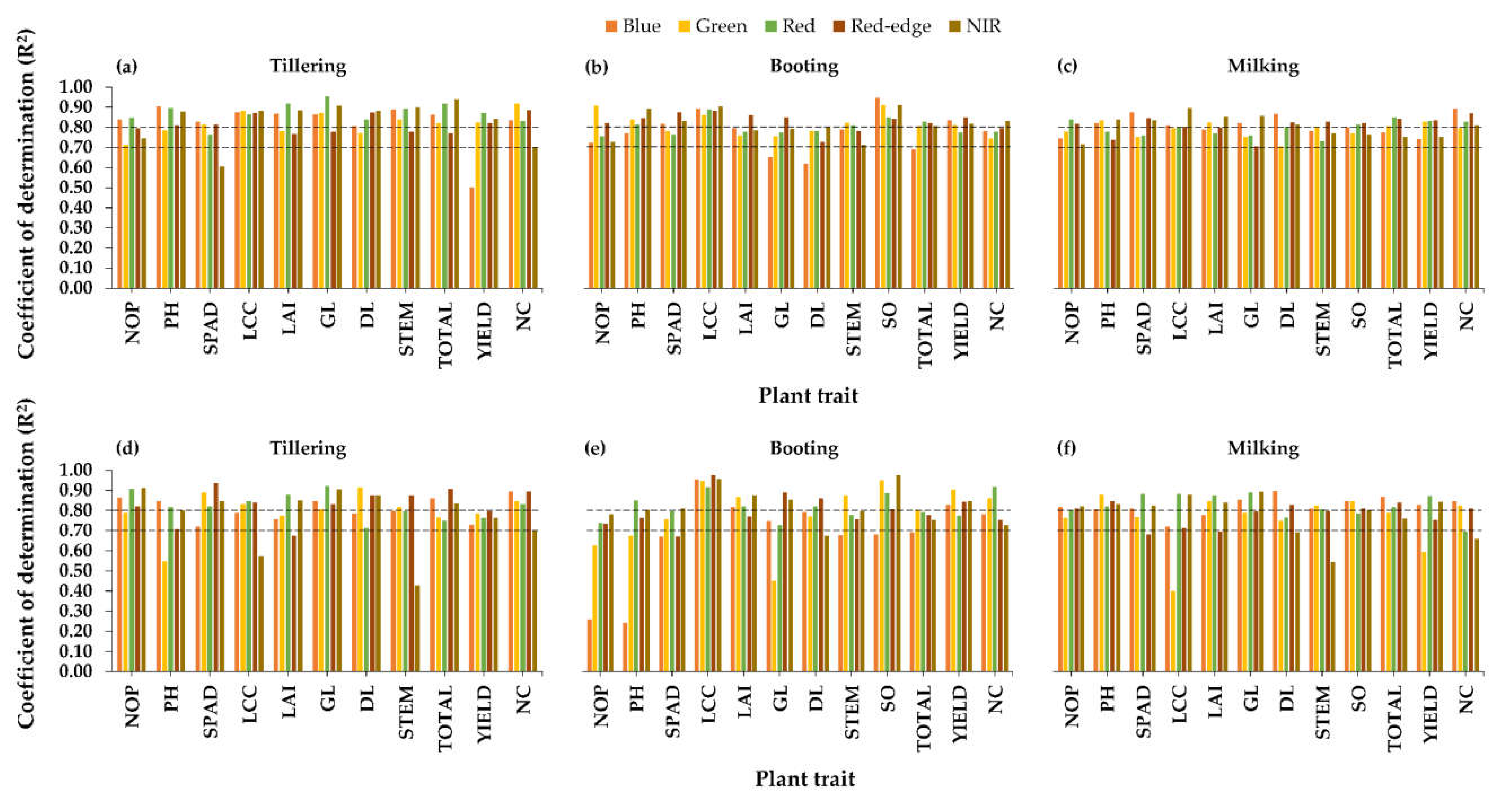
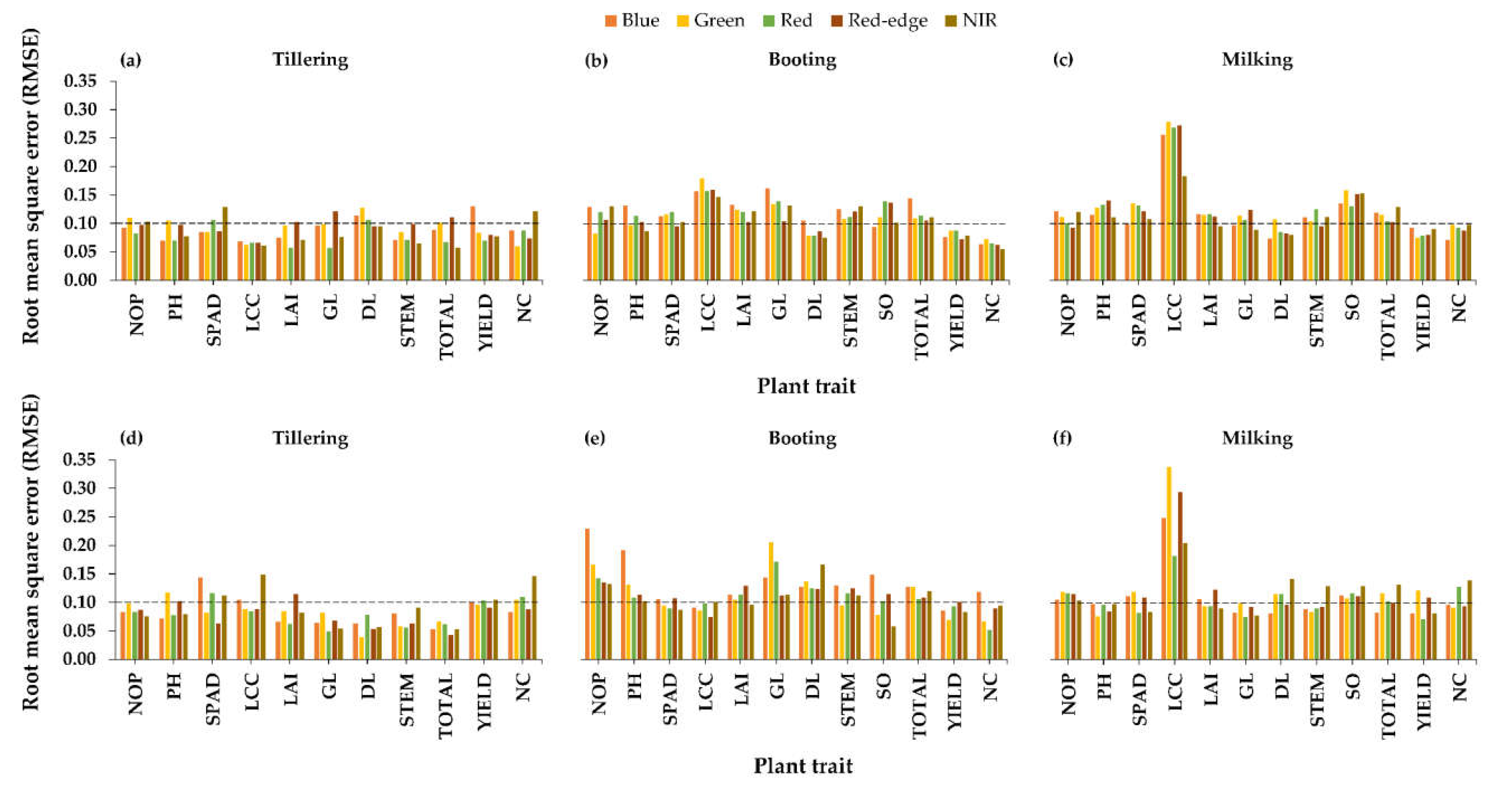
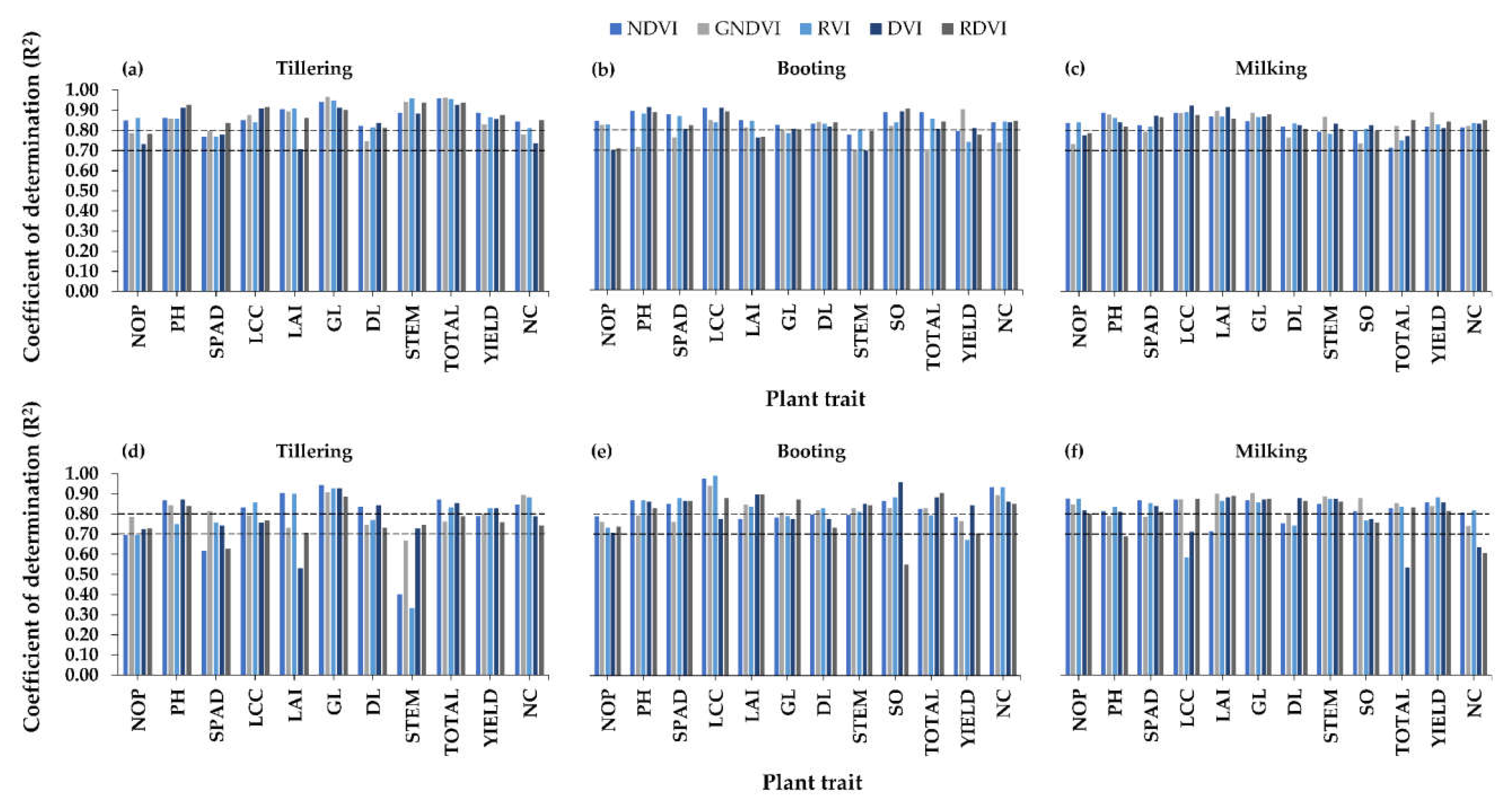
3.2. Relationships between Multispectral Images and Plant Traits

The R² and RMSE values obtained in this study signified that the use of multispectral UAV sensor integrated with machine learning algorithms could produce strong estimations of rice plant traits across rice growth stages (Figure 2, Figure 3, Figure 4, Figure 5, Figure 6 and Figure 7). Figure 2, Figure 4 and Figure 6 visually display that out of 1190 combinations of plant traits, indices, growth stages and datasets (training or testing) tested, 92.02% plant traits obtained an R² of > 0.70. Additionally, Figure 3, Figure 5 and Figure 7 portray that 54.87% of the RMSEs were below 0.10.

3.2.1. Relationships between Raw Bands and Plant Traits

The R² and RMSE values generated between plant traits and raw bands for all rice growth stages are tabulated in Figure 2a–f and Figure 3a–f for training and testing, respectively. At the tillering stage, regardless of plant traits except for the YIELD, PH, LCC and STEM biomass, all raw bands resulted in R² values ≥ 0.60 and RMSE values ≤ 0.15, with red and red-edge bands exhibiting R² values ≥ 0.68 with similar RMSE values ≤ 0.12, respectively. On the other hand, both booting and milking stages recorded R² values ≥ 0.62 and RMSE ranging from 0.05–0.30 for all plant traits and bands, with a few exceptions as follows: the blue band for NOP and PH (booting stage, testing datasets), green band for GL (booting stage, testing datasets), LCC and YIELD readings (milking stage, testing datasets), and NIR for STEM biomass (milking stage, testing datasets).

At the tillering stage, across the raw bands, five plant traits, i.e., NOP, GL, DL, TOTAL biomass, and NC obtained high R² values, i.e., 0.70–0.95 (RMSE ≤ 0.15) (Figure 2 and Figure 3). Moderate R² (0.50–0.94) and comparable RMSE (≤0.15) values were obtained for PH, SPAD, LCC, LAI and YIELD for all raw bands. At the booting stages, the models’ performance for all plant traits depicted R² values of 0.62–0.97 (RMSE ≤ 0.17), including a group of plant traits that obtained higher accuracies, i.e., LCC, LAI, YIELD and NC (R² = 0.73–0.98, RMSE ≤ 0.18), except for a group of plant traits that had extremely low testing accuracies, i.e., NOP (blue band), PH (blue band) and GL (green band). Nevertheless, at the milking stage, the models’ performance for all plant traits depicted a decreasing trend compared to its performance at tillering and booting, i.e., R² values of 0.66–0.90 and RMSE values of 0.07–0.30 with the exclusion of LCC and YIELD (red band, testing datasets) and STEM (NIR band, testing datasets). NOP, PH, GL, SO and TOTAL biomass illustrated strong R² values for both training and testing datasets, i.e., 0.71–0.89 (RMSE ≤ 0.16).

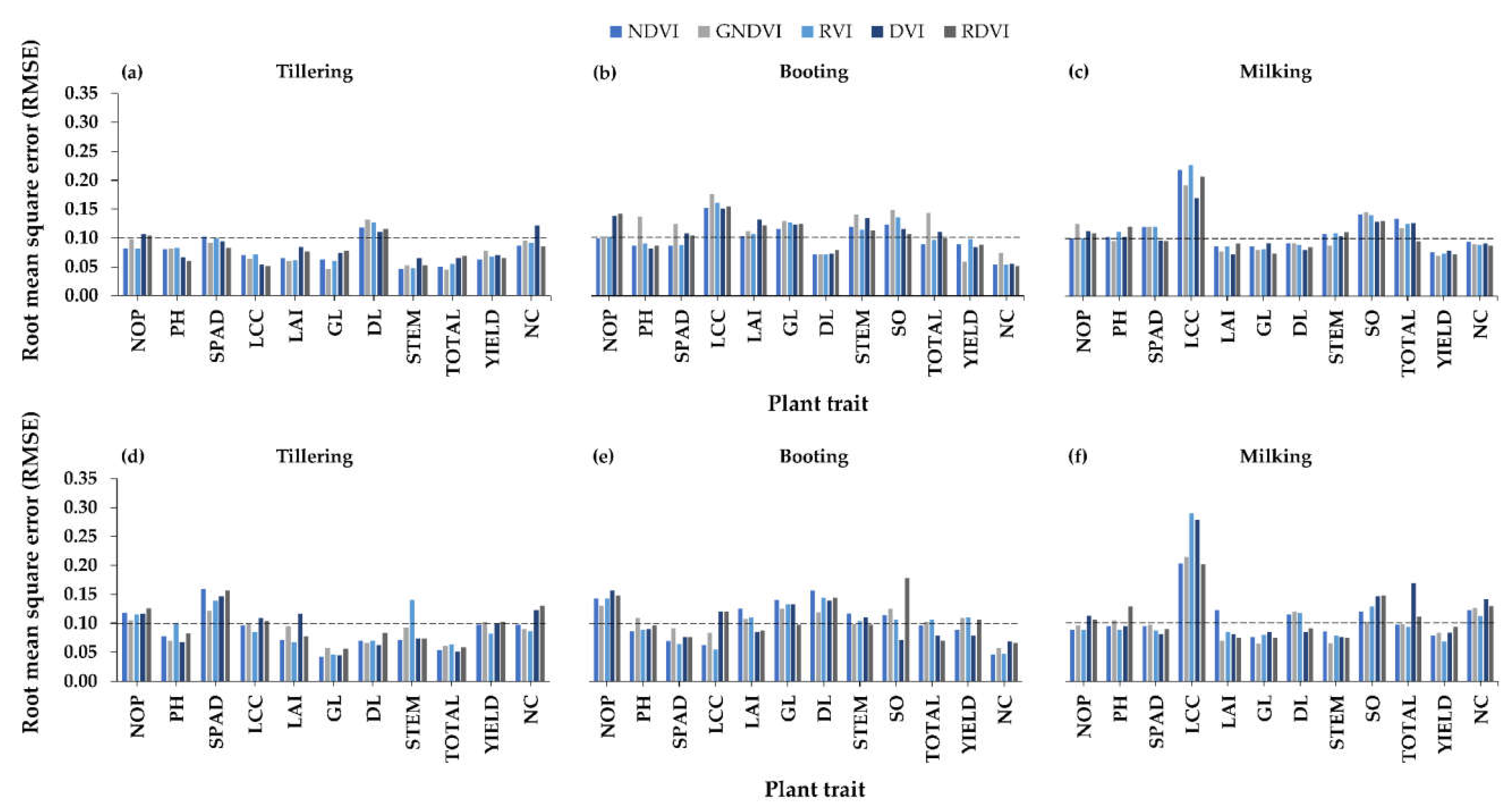
3.2.2. Relationships between Visible-NIR Indices and Plant Traits

Figure 4a–f and Figure 5a–f depict the evaluation of visible and NIR indices for estimating plant trait values at different rice growth stages for training and testing datasets, respectively. In general, all indices illustrated the ability to model all tested plant traits with R² values ≥ 0.61 and RMSE ≤ 0.30 for all growth stages with a few exclusions as follows: NDVI and RVI for STEM (tillering stage, testing dataset), DVI for LAI (tillering stage, testing dataset), RDVI for SO (booting stage, testing dataset), RVI for LCC (milking stage, testing dataset) and DVI for TOTAL biomass (milking stage, testing dataset). On the other hand, only one index, i.e., GNDVI (R² = 0.67–0.97 and RMSE = 0.05–0.21) demonstrated consistent model performance for both training and testing datasets for all tested plant traits and growth stages.

At the tillering stage, for both training and testing datasets, GL models yielded the highest model performance for all indices (R² = 0.89–0.97, RMSE ≤ 0.07), while STEM biomass and LAI were the worst performing models, especially those evaluated with NDVI and RVI (R² = 0.33–0.96, RMSE ≤ 0.12) and DVI (R² = 0.53–0.90, RMSE ≤ 0.12), respectively (Figure 4 and Figure 5). The remaining plant traits illustrated moderate to strong model accuracies (R² = 0.61–0.99, RMSE ≤ 0.29). A contrasting observation could be made at the booting stage where many plant traits illustrated a strong relationship (R² values ≥ 0.70 and RMSE ≤ 0.17) with visible-NIR indices, i.e., NOP, PH, SPAD, LCC, LAI, GL, DL and NC. Nonetheless, it was noted that the model performance for NC was substantially higher during the testing stage (R² = 0.85–0.94, RMSE ≤ 0.07) than during the training (R² = 0.74–0.84, RMSE ≤ 0.07). Finally, at the milking stage, only two plant traits, i.e., GL and YIELD demonstrated model R² values ≥ 0.81 for all indices (RMSE ≤ 0.09), while other plant traits were modelled satisfactorily with all indices as previously mentioned.

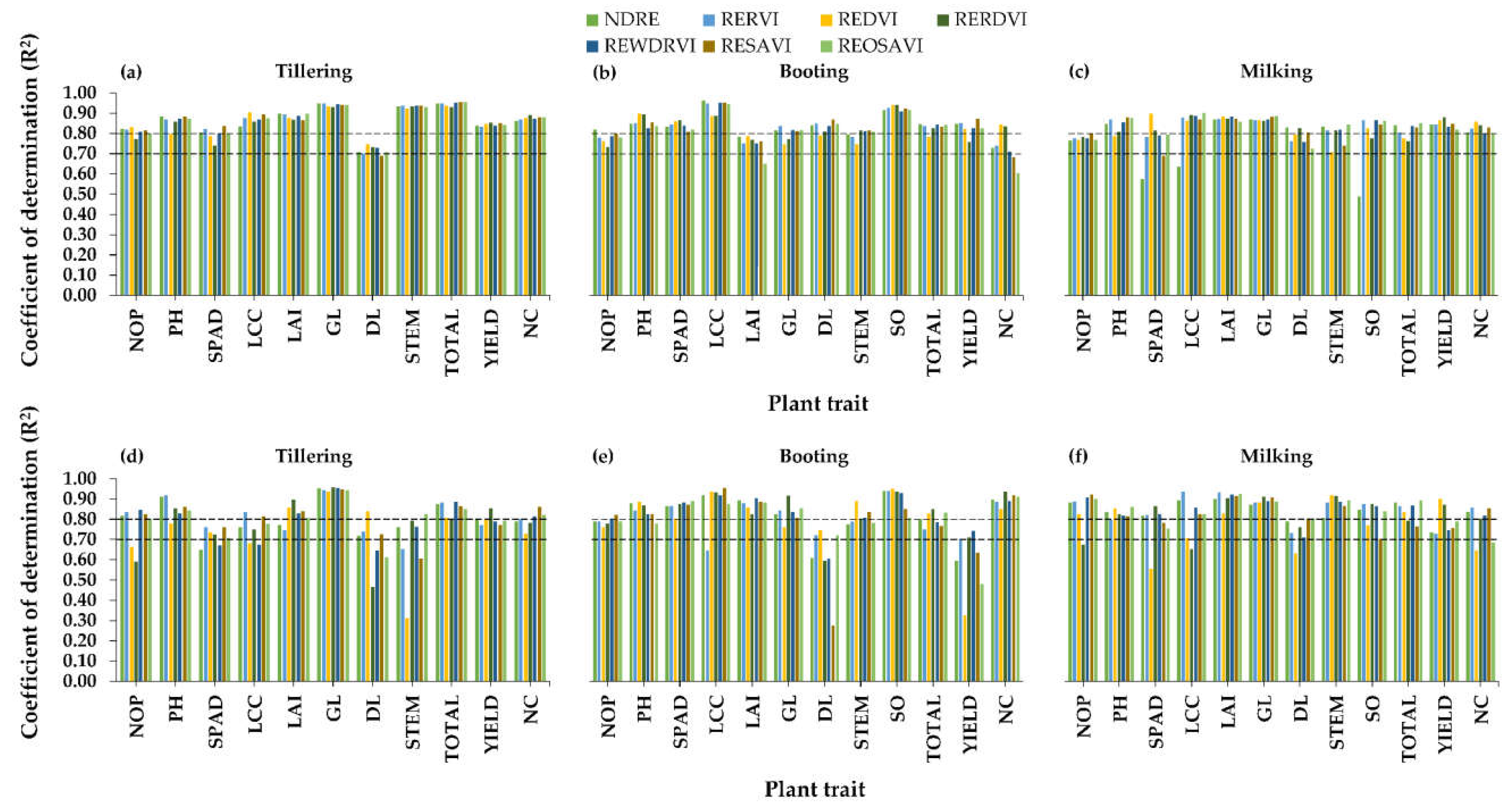
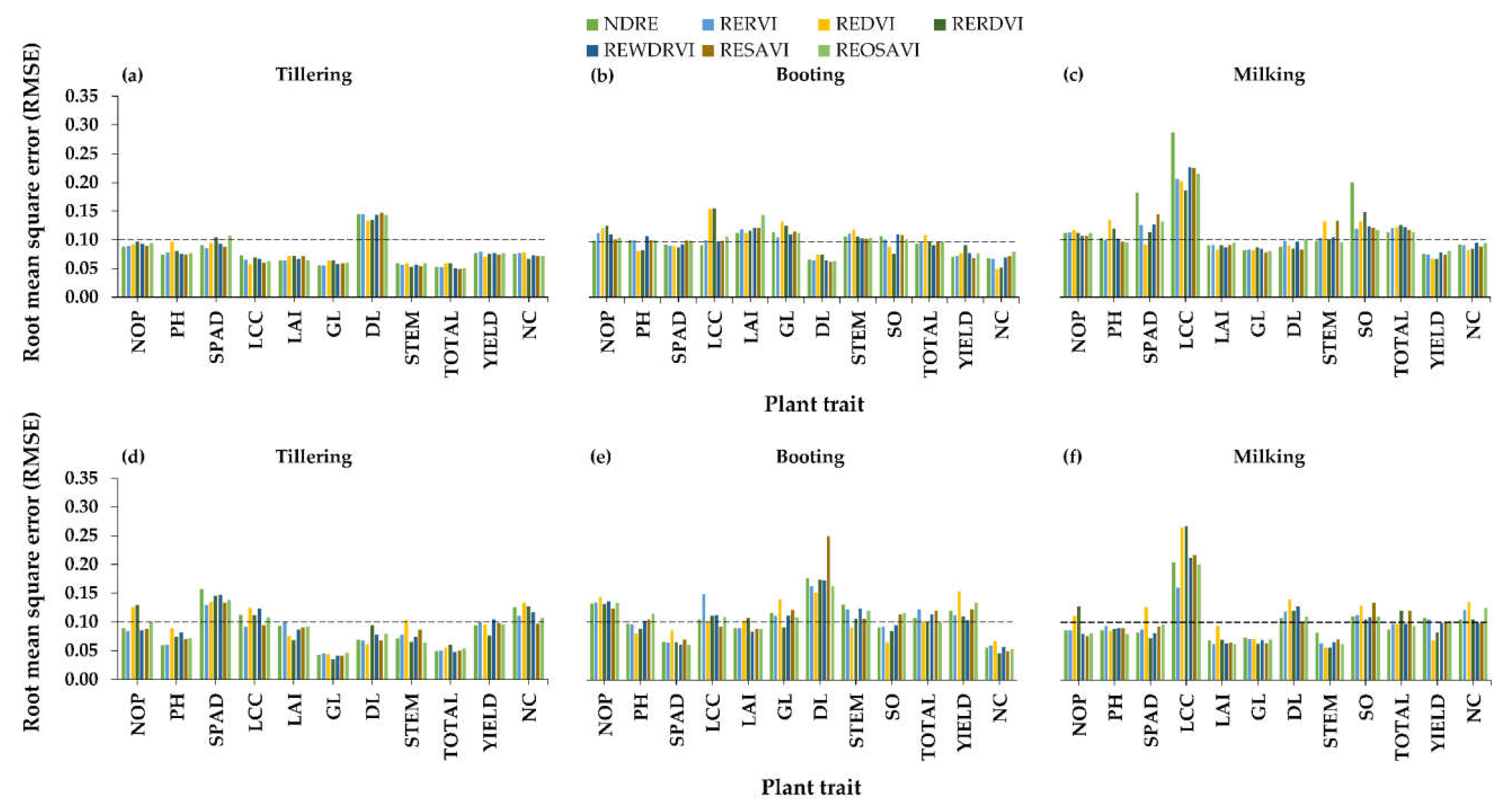
3.2.3. Relationships between Red-Edge-NIR Indices and Plant Traits

Figure 6a–f and Figure 7a–f show the R² and RMSE values for the relationship modelled between the red-edge and NIR indices and plant traits for the training and testing datasets for all growth stages. All seven red-edge indices examined demonstrated reasonable model performance (R² = 0.60–0.96 and RMSE ≤ 0.31) for all plant traits and growth stages across the training and testing datasets. Nevertheless, lower accuracies (R² = 0.27–0.59 and RMSE ≤ 0.25) were observed for these occasions: REDVI for STEM biomass (tillering stage, testing dataset), RERDVI for NOP and DL (tillering stage, testing dataset), NDRE, REDVI and REOSAVI for YIELD (booting stage, testing dataset), RERDVI and RESAVI for DL (booting stage, testing dataset), NDRE for SPAD and SO (milking stage, training dataset) and REDVI for SPAD (milking, testing dataset).

At the tillering stage, six plant traits, i.e., PH, LAI, GL biomass, TOTAL biomass, YIELD and NC exhibited strong R² values = 0.73–0.96 for all indices (RMSE ≤ 0.13) (Figure 7 and Figure 8), with a GL that consistently illustrated the highest R² values, i.e., 0.93–0.96. With the exception previously mentioned, other remaining plant traits had moderate to strong model accuracies (R² = 0.60–0.96, RMSE ≤ 0.16) for both training and testing models. At the booting stage, NOP, PH, SPAD, and four type of biomass, i.e., GL, STEM, SO and TOTAL biomass models illustrated strong performances for both training and testing datasets, i.e., R² values ≥ 0.74 for all indices (RMSE ≤ 0.14). On the other hand, other plant traits, i.e., LCC, LAI, DL, YIELD and NC showed low to strong accuracies for all indices (R² = 0.27–0.97, RMSE ≤ 0.25). At the milking stage, LAI and GL biomass depicted consistent models for all indices for both training and testing with R² ≥ 0.83 (RMSE ≤ 0.10), and followed by other plant traits such as PH, STEM and TOTAL biomass, and YIELD (R² = 0.71–0.92, RMSE ≤ 0.13).

3.3. Performance of the Random Forest-AdaBoost Algorithms

As regards the machine learning algorithms, Figure 8 shows that the residuals between the training and testing R² and RMSE across plant traits and growth stages were positive and negative in an almost equal measure and were very close to the 0 value, despite the fact that there was a slight tendency towards the positive direction that was reflected through the outliers.

4. Discussion

4.1. Performance of Plant Traits Estimations

Further investigations on the testing datasets trait score (R² ≥ 0.80) (

Table 4. Index and trait score for all plant traits and indices at tillering.

Growth Stage	Plant Trait	Raw Band					Visible-NIR Indices					Red-Edge-NIR Indices							Trait Score
		Blue	Green	Red	Red-edge	NIR	NDVI	GNDVI	RVI	DVI	RDVI	NDRE	RERVI	REDVI	RERDVI	REWDRVI	RESAVI	REOSAVI
Tillering	NOP	1	0	1	1	1	0	0	0	0	0	1	1	0	0	1	1	0	8
	PH	1	0	1	0	0	1	1	0	1	1	1	1	0	1	1	1	1	12
	SPAD	0	1	1	1	1	0	1	0	0	0	0	0	0	0	0	0	0	5
	LCC	0	1	1	1	0	1	0	1	0	0	0	1	0	0	0	1	0	7
	LAI	0	0	1	0	1	1	0	1	0	0	0	0	1	1	1	1	1	9
	GL	1	1	1	1	1	1	1	1	1	1	1	1	1	1	1	1	1	17
	DL	0	1	0	1	1	1	0	0	1	0	0	0	1	0	0	0	0	6
	STEM	0	1	0	1	0	0	0	0	0	0	0	0	0	0	0	0	1	3
	TOTAL	1	0	0	1	1	1	0	1	1	0	1	1	1	0	1	1	1	12
	YIELD	0	0	0	0	0	0	1	1	1	0	1	0	1	1	0	0	0	6
	NC	1	1	1	1	0	1	1	1	0	0	0	1	0	0	1	1	1	11
	Index score	5	6	7	8	6	7	5	6	5	2	5	6	5	4	6	7	6

,

Table 5. Index and trait score for all plant traits and indices at booting.

Growth Stage	Plant Trait	Raw Band					Visible-NIR Indices					Red-Edge-NIR Indices							Trait Score
		Blue	Green	Red	Red-edge	NIR	NDVI	GNDVI	RVI	DVI	RDVI	NDRE	RERVI	REDVI	RERDVI	REWDRVI	RESAVI	REOSAVI
Booting	NOP	0	0	0	0	0	0	0	0	0	0	0	0	0	0	1	1	0	2
	PH	0	0	1	0	1	1	0	1	1	1	1	1	1	1	1	1	0	12
	SPAD	0	0	0	0	1	1	0	1	1	1	1	1	1	1	1	1	1	12
	LCC	1	1	1	1	1	1	1	1	0	1	1	0	1	1	1	1	1	15
	LAI	1	1	1	0	1	0	1	1	1	1	1	1	1	1	1	1	1	15
	GL	0	0	0	1	1	0	1	0	0	1	1	1	0	1	1	1	1	10
	DL	0	0	1	1	0	0	1	1	0	0	0	0	0	0	0	0	0	4
	STEM	0	1	0	0	0	0	1	1	1	1	0	0	1	1	1	1	0	9
	SO	0	1	1	1	1	1	1	1	1	0	1	1	1	1	1	1	1	15
	TOTAL	0	0	0	0	0	1	1	0	1	1	0	0	1	1	0	0	1	7
	YIELD	1	1	0	1	1	0	0	0	1	0	0	0	0	0	0	0	0	5
	NC	0	1	1	0	0	1	1	1	1	1	1	1	1	1	1	1	1	14
	Index score	3	6	6	5	7	6	8	8	8	8	7	6	8	9	8	8	7

and

Table 6. Index and trait score for all plant traits and indices at milking.

Growth Stage	Plant Trait	Raw Band					Visible Indices					Red-Edge-NIR Indices							Trait Score
		Blue	Green	Red	Red-edge	NIR	NDVI	GNDVI	RVI	DVI	RDVI	NDRE	RERVI	REDVI	RERDVI	REWDRVI	RESAVI	REOSAVI
Milking	NOP	1	0	1	1	1	1	1	1	1	0	1	1	1	0	1	1	1	14
	PH	1	1	1	1	1	1	0	1	1	0	1	0	1	1	1	1	1	14
	SPAD	1	0	1	0	1	1	0	1	1	1	1	1	0	1	1	0	0	11
	LCC	0	0	1	0	1	1	1	0	0	1	1	1	0	0	1	1	1	10
	LAI	0	1	1	0	1	0	1	1	1	1	1	1	1	1	1	1	1	14
	GL	1	0	1	0	1	1	1	1	1	1	1	1	1	1	1	1	1	15
	DL	1	0	0	1	0	0	1	0	1	1	0	0	0	0	0	1	1	7
	STEM	1	1	1	0	0	1	1	1	1	1	1	1	1	1	1	1	1	15
	SO	1	1	0	1	0	1	1	0	0	0	1	1	0	1	1	0	1	10
	TOTAL	1	0	1	1	0	1	1	1	0	1	1	1	1	0	1	0	1	12
	YIELD	1	0	1	0	1	1	1	1	1	1	0	0	1	1	0	0	0	10
	NC	1	1	0	1	0	1	0	1	0	0	1	1	0	1	1	1	0	10
	Index score	10	5	9	6	7	10	9	9	8	8	10	9	7	8	10	8	9
TOTAL SCORE		18	17	22	19	20	23	22	23	21	18	22	21	20	21	24	23	22

) illustrated that four plant traits could be estimated at all growth stages using most of the indices with R² ≥ 0.80, i.e., PH (12, 12 and 14), GL biomass (17, 10, 15), SO biomass (15 and 10) and NC (11, 14 and 10). A general observation that could be made is that these four traits are sensitive to a variety of indices, while the remaining plant traits are limitedly sensitive to a few indices.

Good estimates of PH using the indices suggest that this approach may be an alternative to the robust DSM or CSM [13,14], and this finding warrants further investigation. The maximum R² values obtained across the season (0.89 to 0.92) were in agreement with those found by Jiang et al. [13] (R² < 0.85, the highest was 0.91), yet with much lower RMSE values (0.06–0.19 m versus 0.27 m). The GL biomass estimation, while satisfactory for tillering and milking stages, was slightly lower during the booting stage. The low trait score at the booting stage for this plant trait was hypothesized to be due to increased greenness (high SPAD and LCC readings) and biomass which saturated most of the indices, especially in the raw bands and visible-NIR indices groups (Table 3 and Figure 9) [37,38]. The LAI findings are contradictory to the findings of GL biomass; this plant trait demonstrated high accuracy estimations during booting and milking stages. This observation could be attributed to the higher LAI at these two stages, as compared to tillering. At tillering, since the LAI was still low, the surrounding inundated water might contribute to the observed signals (Figure 9).

In this study, the SO estimations were better than the YIELD prediction, given the presence of the storage organ during the booting and milking stages (Figure 9). The YIELD prediction, on the hand, was best conducted during the milking (trait score = 10), compared to the tillering and booting stages (trait score = 6 and 5, respectively), due to the closer date to actual harvesting, and thus, the presence of mature storage organs. Among the plant traits examined, the previous literature showed that the estimation of NC with high accuracy is often not straightforward [36,40]. For instance, Zheng et al. [40], in a study to estimate rice leaf NC using multispectral UAV images, achieved RMSEs ranging from 0.17–0.27% for individual growth stages that they tested. On the other hand, our study obtained RMSEs ranging from 0.05–0.15% for the NC for most of the raw bands and indices tested across individual growth stages. It is worth noting that the NC in this study had a narrow range, indicating that the indices and algorithms tested were sensitive for differentiating the small variations in the NC.

It was also found that the trait scores of LCC were higher than the SPAD, especially during tillering and booting, despite both being indicators of leaf greenness, relative chlorophyll content, or nitrogen content. Both SPAD and LCC readings displayed a sensitivity towards growth stages, given the highest trait scores during booting, followed by milking and tillering stages. Their readings are known to be influenced by different crop growth stages, nitrogen treatments, crop cultivars and the point of measurement on a leaf blade, as emphasized by Furuya [58], Lin et al. [59] and Islam et al. [60]. On the other hand, throughout the growth stages, the estimation of DL biomass and NOP could be conducted using only eight indices or less, except for NOP during the milking stage. Additionally, STEM estimation at the tillering stage and TOTAL biomass estimation at the booting stage were also unsatisfactory; three and seven indices, respectively. The limitation in estimating the DL and STEM biomass might be due to the location of the dead leaves and stems, which are deeper in the canopy, while the response of the optical sensor is mostly sensible from the top layer of canopy rather than the entire canopy [61]. Furthermore, poor NOP estimations might be due to the broadcasting method that possibly caused the non-uniformed distributions of seeds, and thus, rice canopies. Compared to the study conducted by Wu et al. [15], our best R² for NOP estimation (testing, during the milking) was slightly lower, i.e., 0.92 versus 0.94.

4.2. Best Vegetation Indices for Plant Traits Estimations

Overall, the total index score demonstrated that the raw bands and indices were stage-specific, However, red from the raw bands group (total index score: 22), NDVI and RVI from the visible indices group (total index score: 23), and REWDRVI and RESAVI from the red-edge indices group (total index score: 24 and 23, respectively) had the best performance in estimating all plant traits across growth stages (Table 4, Table 5 and Table 6). These index scores implied that 70% of the plant traits across three growth stages could be estimated robustly with an R² ≥ 0.80. A single band was observed, i.e., a red band was depicted with comparable performance to the indices, especially during tillering and milking (Table 4 and Table 6). Throughout the stages, the red band displayed sensitivities, especially for non-biomass traits. This result contradicts the findings reported by other researchers [11], who found that the red wavelength is prone to LAI and biomass saturation in comparison to the green and red-edge. We hypothesize that this might be due to plant conditions, whereby at the vegetative stages—especially the tillering and early booting stages—young plants are photosynthetically active and chlorophyll filling, thus, absorbing more red lights.

Furthermore, the NDVI and RVI illustrated better performance than other indices in the visible indices group, especially at tillering. While these two indices were sensitive for greenness indicators, i.e., LCC and NC, their sensitivity towards the biomass component appeared to be random. On the other hand, the performance of NDVI was the poorest at the booting stage (Table 5), especially for LAI and GL biomass given the highest values of these two traits, although RVI performed best at this stage. In this study, the poor performance of the NDVI might be due to the red band, considering that the sensitivities were slightly lower compared to NIR (Table 5). The inconsistency of NDVI was reported by Cheng et al. [39], whereby the index performed the best for estimating leaf biomass (R² = 0.76) but demonstrated a slightly lower performance for stem and total biomass (R² = 0.68). Din et al. [62] also found that the performance of RVI and NDVI for the LAI estimation was subject to the different crop stages tested; for the RVI, R² = 0.92 and 0.72 at elongation, 0.94 and 0.49 at booting and 0.80 and 0.39 at heading and for the NDVI, R² = 0.89 and 0.77 at elongation, 0.67 and 0.69 at booting and 0.75 and 0.48 at heading. Zhou et al. [11] also illustrated that rice yield estimation from NDVI and RVI varied according to differences in growth stages; with the highest found at initial booting and booting stages (r = 0.42–0.66) compared to other stages (r = 0.21–0.61). On the other hand, other indices in the group performed well at both booting and milking stages.

From the red-edge-NIR index group, REWDRVI and RESAVI performed slightly better than the others. The REWDRVI was found to be more sensitive than the other red-edge indices at milking and tillering, despite its consistent insensitivity to DL biomass and YIELD prediction. RESAVI, on the hand, performed consistently throughout all growth stages, with limited ability to predict YIELD, and estimate DL biomass and SPAD. Kanke et al. [38] attributed the differences in accuracy among the red-edge band and indices such as RERVI, NDRE, RERDVI, REDVI and RESAVI, obtained from a spectroradiometer, to the transformation of the red-edge and NIR reflectance, i.e., ratio or normalized form that could affect the sensitivity of the indices due to narrowing or widening effects. Although researchers such as Cao et al. [36] reported the better performance of the red-edge based index compared to the visible-NIR indices, due to the lower level of signal saturation in comparison to the red wavelength, this study observed that the visible-NIR indices generally performed equally satisfactorily to the red-edge-NIR indices. This finding is advantageous given the absence of red-edge bands, the conventional NDVI and RVI could serve as an alternative.

Among the bands and indices tested, two bands, i.e., blue and green, and one index, i.e., RDVI, demonstrated ≤50% performances or total index scores below 18 in estimating plant traits. The remaining bands or indices, i.e., red-edge, NIR, NDVI, GNDVI, DVI, NDRE, RERVI, REDVI, RERDVI, and REOSAVI performed reasonably, with a total index score ranging from 19 to 22. A striking similarity between these poor and reasonably performing indices was that they were insensitive to NOP, DL and STEM biomass, and YIELD at the tillering stage (Table 4).

4.3. Best Rice Growth Stage for Plant Trait Estimations

Although plant trait estimations were trait-stage dependent, according to the trait scores, milking is the best growth stage for conducting plant phenotyping or obtaining the maximum plant trait estimation number. This is followed by booting and tillering (Table 4, Table 5 and Table 6). The trait score for all plant traits at milking was 10 or above, except for the NOP that could be estimated using only seven indices. Five plant traits could be estimated using almost all the indices with an R² ≥ 0.80, i.e., NOP, PH, LAI, GL biomass and STEM biomass. The trait score for plant traits during the milking and booting stages were also comparable for these plant traits: PH, SPAD, LAI and DL biomass. Nevertheless, three plant traits were better estimated at the booting stage, i.e., LCC, SO biomass and NC. Although at tillering, only four plant traits could be estimated with ≥10 indices with an R² ≥ 0.80, i.e., PH, GL biomass, TOTAL biomass and NC scores were either comparable or better than milking. These accuracy trends were believed to be affected by the crop physiological state (Figure 9). At tillering, seven traits had a score below 10, and the presence of inundated water possibly contributed to these low trait scores (Figure 9a). Nevertheless, the GL and TOTAL biomass estimation at this stage was highly desirable, owing to the greenness of the plants, as can be seen in Figure 9a and the dominance of GL biomass that was almost 46% of the TOTAL biomass. However, during booting, the accuracy of the GL and TOTAL biomass estimation slightly decreased, perhaps due to saturation of the signals resulting from the greatest biomass and also the higher proportions of non-leaf biomass components (Table 3). At milking, the accuracies were slightly decreased, perhaps due to the domination of storage organs and stems (Table 3). The biomass result contradicts that determined by Zheng et al. [7] and Lu et al. [6], who reported the best result at the pre-heading and panicle initiation stages, respectively.

LCC and NC estimations were the best at the booting stage, perhaps due to the strongest green color being observed for plants at this stage (Figure 9b). This result is comparable to the findings of Zheng et al. [7], who best estimated LNA at the same growth stage. Zheng et al. [40], on the other hand, illustrated that the best growth stage to estimate rice leaf - and plant N concentrations depend on the season; at the filling stage (for both traits) in one of the two tested years, while at the heading stage for leaf N, and the filling stage for plant N in another year. In our study, LAI was best estimated at both the booting and milking stages. This is similar to the findings by Lu et al. [6], who illustrated that the optimal stage for LAI estimation was panicle initiation, where both stages occur in the reproductive stage. Finally, of equal importance, YIELD prediction was best conducted during the milking stage, whereby the presence of storage organs was the maximum (Table 3, Figure 9c). This result, nevertheless, contradicted the findings by Zhou et al. [11], who demonstrated that grain yield estimation was best conducted at the booting stage.

4.4. Performance of the Random Forest-AdaBoost Algorithms

Box plot analysis suggested the stability of the RFA performance between the training and testing models in avoiding general model overfitting or underfitting. These low errors were possibly due to the optimization of Adaboost-supported hyperparameters such as the split sample predictor that accurately predicted the data across all stages, plant traits and indices. Additionally, the re-weighting technique by the AdaBoost could have produced more uncorrelated trees that maximize the generalization performance. The ($\ln \frac{1}{{\mathsf{\omega }}_i}$) weightage of the AdaBoost was able to reduce the OOB data (or unused data) to close to zero and eventually, this will help the weak learners to learn better in order to improve model performance [29]. In comparison, RF produces high values of OOB that are approximately one third (or 36%) of the actual data total, which could reduce the prediction accuracy. The ability of AdaBoost to minimize the prediction error is further supported by the high accuracies of plant trait estimation. As previously mentioned, only 7.98% of the estimations of plant traits obtained an R² < 0.70. The low accuracy estimation of certain plant traits could be due to the large margin errors between the RF learning algorithms and random data from the AdaBoost. Specifically, the former will continuously grow in complexity with the size of training dataset but the continuous iterations can compromise the latter. Furthermore, the performance of the RFA in this study could be considered better than other algorithms, such as PLS and ANN, which reported R² values of 0.64 and 0.73, respectively, for LAI estimation across rice growth stages [21] (our study obtained the highest testing R² value of 0.93) or RF for estimating rice biomass and panicle biomass, for which R² values of 0.90 and 0.64 were determined, respectively [10] (our study obtained the highest testing R² = 0.90 and 0.97, respectively). The same is true for stepwise MLR algorithms, which obtained R² = 0.70 for rice foliar NC [40] (our study obtained the highest testing R² = 0.94).

5. Conclusions

Significant progress has been made in terms of the combination of remote sensing and machine learning technologies for plant phenotyping. However, significant limitations persist as regards prediction accuracy and data overfitting/underfitting. Additionally, few studies have comprehensively evaluated many plant traits from multispectral cameras onboard UAV platforms.

Our study attempted to, firstly, evaluate twelve rice plant traits that could effectively be estimated or predicted from aerial unmanned vehicle (UAV) based multispectral images. Secondly, we attempted to introduce RFA algorithms as an optimization approach to reduce data overfit/underfitting for estimating plant traits. Among the plant traits, PH, GL and SO biomass, and NC were well estimated with a coefficient of determination (R²) above 0.80 and root mean square error (RMSE) below 0.22. In comparing the bands and indices, red, NDVI, RVI, REWDRVI and RESAVI were remarkable in estimating all plant traits at tillering to milking stages with R² ranging from 0.80–0.92 (RMSE = 0.05–0.18), 0.80–0.97 (RMSE = 0.04–0.20), 0.81–0.99 (RMSE = 0.05–0.15), 0.80–0.95 (RMSE = 0.04–0.21) and 0.80–0.96 (RMSE = 0.04–0.22), respectively. Milking was found to be the best growth stage for conducting an estimation of plant traits. Additionally, this study found that the RFA algorithm has a high potential to estimate rice plant traits with high R² values (92.02% of the plant traits estimations obtained R² > 0.70) and low residuals (RMSE = 0.03–0.34) for the training and testing models, confirming its ability to reduce error without overfitting or underfitting. Collectively, these results signify a new opportunity for rice phenotyping via integration of the UAV-multispectral method and machine learning.

The limitations of this study include the sample size which does not address the effects of cultivars or nitrogen. In the future, research could be undertaken to classify the effects of cultivars and nitrogen treatments on plant traits for further phenotyping studies. This study also did not consider the uptake of technology by the machine learning tools developed, as was done in the study by Vecchio et al. [63].

References

1. Kefauver, S.C.; Vicente, R.; Vergara-Díaz, O.; Fernandez-Gallego, J.A.; Kerfal, S.; Lopez, A.; Melichar, J.P.; Serret Molins, M.D.; Araus, J.L. Comparative UAV and field phenotyping to assess yield and nitrogen use efficiency in hybrid and conventional barley. Front. Plant Sci. 2017, 8, 1733. [Google Scholar] [CrossRef] [PubMed]
2. Tattaris, M.; Reynolds, M.P.; Chapman, S.C. A direct comparison of remote sensing approaches for high-throughput phenotyping in plant breeding. Front. Plant Sci. 2017, 7, 1131. [Google Scholar] [CrossRef] [PubMed]
3. Yang, G.; Liu, J.; Zhao, C.; Li, Z.; Huang, Y.; Yu, H.; Xu, B.; Yang, X.; Zhu, D.; Zhang, X.; et al. Unmanned aerial vehicle remote sensing for field-based crop phenotyping: Current status and perspectives. Front. Plant Sci. 2017, 8, 1111. [Google Scholar] [CrossRef]
4. Watanabe, K.; Guo, W.; Arai, K.; Takanashi, H.; Kajiya-Kanegae, H.; Kobayashi, M.; Yano, K.; Tokunaga, T.; Fujiwara, T.; Tsutsumi, N.; et al. High-throughput phenotyping of sorghum plant height using an unmanned aerial vehicle and its application to genomic prediction modeling. Front. Plant Sci. 2017, 8, 421. [Google Scholar] [CrossRef] [Green Version]
5. Chawade, A.; van Ham, J.; Blomquist, H.; Bagge, O.; Alexandersson, E.; Ortiz, R. High-throughput field-phynotyping tools for plant breeding and precision agriculture. Agronomy 2019, 9, 258. [Google Scholar] [CrossRef] [Green Version]
6. Lu, J.; Miao, Y.; Huang, Y.; Shi, W.; Hu, X.; Wang, X.; Wan, J. Evaluating an Unmanned Aerial Vehicle-Based Remote Sensing System for Estimation of Rice Nitrogen Status. In Proceedings of the 4th International Conference on Agro-Geoinformatics (Agro-geoinformatics), Istanbul, Turkey, 20–24 July 2015; pp. 198–203. [Google Scholar] [CrossRef]
7. Zheng, H.; Cheng, T.; Li, D.; Zhou, X.; Yao, X.; Tian, Y.; Cao, W.; Zhu, Y. Evaluation of RGB, color-infrared and multispectral images acquired from unmanned aerial systems for the estimation of nitrogen accumulation in rice. Remote Sens. 2018, 10, 824. [Google Scholar] [CrossRef] [Green Version]
8. Li, S.; Ding, X.; Kuang, Q.; Ata-UI-Karim, S.T.; Cheng, T.; Liu, X.; Tian, Y.; Zhu, Y.; Cao, W.; Cao, Q. Potential of UAV-based active sensing for monitoring rice leaf nitrogen status. Front. Plant Sci. 2018, 14, 1834. [Google Scholar] [CrossRef] [Green Version]
9. Zheng, H.; Cheng, T.; Zhou, M.; Li, D.; Yao, X.; Tian, Y.; Cao, W.; Zhu, Y. Improved estimation of rice aboveground biomass combining textural and spectral analysis of UAV imagery. Precis. Agric. 2019, 20, 611. [Google Scholar] [CrossRef]
10. Cen, H.; Wan, L.; Zhu, J.; Li, Y.; Li, X.; Zhu, Y.; Weng, H.; Wu, W.; Yin, W.; Xu, C.; et al. Dynamic monitoring of biomass of rice under different nitrogen treatments using a lightweight UAV with dual image-frame snapshot cameras. Plant Methods 2019, 15, 32. [Google Scholar] [CrossRef] [PubMed]
11. Zhou, X.; Zheng, H.B.; Xu, X.Q.; He, J.Y.; Ge, X.K.; Yao, X.; Cheng, T.; Zhu, Y.; Cao, W.X.; Tian, Y.C. Predicting grain yield in rice using multi-temporal vegetation indices from UAV-based multispectral and digital imagery. ISPRS J. Photogramm. Remote Sens. 2017, 130, 246. [Google Scholar] [CrossRef]
12. Duan, B.; Fang, S.; Zhu, R.; Wu, X.; Wang, S.; Gong, Y.; Peng, Y. Remote estimation of rice yield with unmanned aerial vehicle (UAV) data and spectral mixture analysis. Front. Plant Sci. 2019, 10, 204. [Google Scholar] [CrossRef] [Green Version]
13. Jiang, Q.; Fang, S.; Peng, Y.; Gong, Y.; Zhu, R.; Wu, X.; Ma, Y.; Duan, B.; Liu, J. UAV-based biomass estimation for rice-combining spectral, TIN-based structural and meteorological features. Remote Sens. 2019, 11, 890. [Google Scholar] [CrossRef] [Green Version]
14. Kawamura, K.; Asai, H.; Yasuda, T.; Khanthavong, P.; Soisouvanh, P.; Phongchanmixay, S. Field phenotyping of plant height in an upland rice field in Laos using low-cost small unmanned aerial vehicles (UAVs). Plant Prod. Sci. 2020, 23, 452. [Google Scholar] [CrossRef]
15. Wu, J.; Yang, G.; Yang, X.; Xu, B.; Han, L.; Zhu, Y. Automatic counting of in situ rice seedlings from UAV images based on a deep fully Convolutional Neural Network. Remote Sens. 2019, 11, 691. [Google Scholar] [CrossRef] [Green Version]
16. Saberioon, M.M.; Gholizadeh, A. Novel approach for estimating nitrogen content in paddy fields using low altitude remote sensing system. Int. Arch. Photogramm. Remote Sens. Spat. Inf. Sci. Isprs Arch. 2016, 1011–1015. [Google Scholar] [CrossRef] [Green Version]
17. Colorado, J.D.; Cera-Bornacelli, N.; Caldas, J.S.; Petro, E.; Rebolledo, M.C.; Cuellar, D.; Calderon, F.; Mondragon, I.F.; Jaramillo-Botero, A. Estimation of nitrogen in rice crops from UAV-captured images. Remote Sens. 2020, 12, 3396. [Google Scholar] [CrossRef]
18. Yuan, S.; Peng, S.; Li, T. Evaluation and application of the ORYZA rice model under different crop managements with high-yielding rice cultivars in central China. Field Crop. Res. 2017, 212, 115. [Google Scholar] [CrossRef]
19. Liu, X.J.; Qiang, C.A.O.; Yuan, Z.F.; Xia, L.I.U.; Wang, X.L.; TIan, Y.C.; Cao, W.X.; Yan, Z.H.U. Leaf area index based nitrogen diagnosis in irrigated lowland rice. J. Integr. Agric. 2018, 17, 111. [Google Scholar] [CrossRef] [Green Version]
20. Tian, G.; Gao, L.; Kong, Y.; Hu, X.; Xie, K.; Zhang, R.; Ling, N.; Shen, Q.; Guo, S. Improving rice population productivity by reducing nitrogen rate and increasing plant density. PLoS ONE 2017, 12, e0182310. [Google Scholar] [CrossRef] [PubMed] [Green Version]
21. Wang, L.; Chang, Q.; Yang, J.; Zhang, X.; Li, F. Estimation of paddy rice leaf area index using machine learning methods based on hyperspectral data from multi-year experiments. PLoS ONE 2018, 13, e0207624. [Google Scholar] [CrossRef] [Green Version]
22. Ndikumana, E.; Ho Tong Minh, D.; Nguyen, D.; Thu, H.; Baghdadi, N.; Courault, D.; Hossard, L.; El Moussawi, I. Estimation of rice height and biomass using multitemporal SAR Sentinel-1 for Camargue, Southern France. Remote Sens. 2018, 10, 1394. [Google Scholar] [CrossRef] [Green Version]
23. Zha, H.; Miao, Y.; Wang, T.; Li, Y.; Zhang, J.; Sun, W.; Feng, Z.; Kusnierek, K. Improving unmanned aerial vehicle remote sensing-based rice nitrogen nutrition index prediction with machine learning. Remote Sens. 2020, 12, 215. [Google Scholar] [CrossRef] [Green Version]
24. Liang, L.; Di, L.; Huang, T.; Wang, J.; Lin, L.; Wang, L.; Yang, M. Estimation of leaf nitrogen content in wheat using new hyperspectral indices and a Random Forest regression algorithm. Remote Sens. 2018, 10, 1940. [Google Scholar] [CrossRef] [Green Version]
25. Sun, J.; Yang, J.; Shi, S.; Chen, B.; Du, L.; Gong, W.; Song, S. Estimating rice leaf nitrogen concentration: Influence of regression algorithms based on passive and active leaf reflectance. Remote Sens. 2017, 9, 951. [Google Scholar] [CrossRef] [Green Version]
26. Yuan, H.; Yang, G.; Li, C.; Wang, Y.; Liu, J.; Yu, H.; Feng, H.; Xu, B.; Zhao, X.; Yang, X. Retrieving soybean leaf area index from unmanned aerial vehicle hyperspectral remote sensing: Analysis of RF, ANN, and SVM regression models. Remote Sens. 2017, 9, 309. [Google Scholar] [CrossRef] [Green Version]
27. Apolo-Apolo, O.E.; Pérez-Ruiz, M.; Martínez-Guanter, J.; Egea, G. A mixed data-based deep neural network to estimate leaf area index in wheat breeding trials. Agronomy 2020, 10, 175. [Google Scholar] [CrossRef] [Green Version]
28. Jeong, J.H.; Resop, J.P.; Mueller, N.D.; Fleisher, D.H.; Yun, K.; Butler, E.E.; Timlin, D.J.; Shim, K.M.; Gerber, J.S.; Reddy, V.R.; et al. Random Forests for global and regional crop yield predictions. PLoS ONE 2016, 11. [Google Scholar] [CrossRef]
29. Mishra, S.; Mishra, D.; Santra, G.H. Adaptive Boosting of weak regressors for forecasting of crop production considering climatic variability: An empirical assessment. J. King Saud Univ. Comp. Info. Sci. 2017, 32, 949. [Google Scholar] [CrossRef]
30. Sun, C.; Feng, L.; Zhang, Z.; Ma, Y.; Crosby, T.; Naber, M.; Wang, Y. Prediction of end-of-season tuber yield and tuber set in potatoes using in-season UAV-based hyperspectral imagery and machine learning. Sensors 2020, 20, 5293. [Google Scholar] [CrossRef]
31. El Bilali, A.; Taleb, A. Prediction of irrigation water quality parameters using machine learning models in a semi-arid environment. J. Saudi Soc. Agric. Sci. 2020, 19, 439. [Google Scholar] [CrossRef]
32. Department of Agriculture (DOA). Paddy Statistics of Malaysia 2014; Statistics Unit, Planning, Information Technology and Communications Division, DOA: Putrajaya, Malaysia, 2015. Available online: http://www.doa.gov.my/index/resources/aktiviti_sumber/sumber_awam/maklumat_pertanian/perangkaan_tanaman/perangkaan_padi_2015.pdf (accessed on 15 January 2021).
33. Meier, U. Growth Stages of Mono- and Dicotyledonous Plants: BBCH Monograph, 2nd ed.; Federal Biological Research Centre for Agriculture and Forestry: Braunschweigh, Germany, 2001; pp. 66–70. [Google Scholar]
34. IRRI-CREMNET (Crop and Resource Management Network). Use of Leaf Colour Chart (LCC) for N Management in Rice; International Rice Research Institute (IRRI) Network Technology: Los Baños, Philippines, 1996. [Google Scholar]
35. Miller, G.L.; Miller, E.E. Determination of nitrogen in biological materials. Anal. Chem. 1948, 20, 481–488. [Google Scholar] [CrossRef]
36. Cao, Q.; Miao, Y.; Wang, H.; Huang, S.; Cheng, S.; Khosla, R.; Jiang, R. Non-destructive estimation of rice plant nitrogen status with Crop Circle multispectral active canopy sensor. Field Crop. Res. 2013, 154, 133. [Google Scholar] [CrossRef]
37. Tian, Y.C.; Gu, K.J.; Chu, X.; Yao, X.; Cao, W.X.; Zhu, Y. Comparison of different hyperspectral vegetation indices for canopy leaf nitrogen concentration estimation in rice. Plant Soil 2014, 376, 193. [Google Scholar] [CrossRef]
38. Kanke, Y.; Tubana, B.; Dalen, M.; Harrell, D. Evaluation of red and red-edge reflectance-based vegetation indices for rice biomass and grain yield prediction models in paddy fields. Precis. Agric. 2016, 17, 507. [Google Scholar] [CrossRef]
39. Cheng, T.; Song, R.; Li, D.; Zhou, K.; Zheng, H.; Yao, X.; Tian, Y.; Cao, W.; Zhu, Y. Spectroscopic estimation of biomass in canopy components of paddy rice using dry matter and chlorophyll indices. Remote Sens. 2017, 9, 319. [Google Scholar] [CrossRef] [Green Version]
40. Zheng, H.; Ma, J.; Zhou, M.; Li, D.; Yao, X.; Cao, W.; Cheng, T. Enhancing the nitrogen signals of rice canopies across critical growth stages through the integration of textural and spectral information from unmanned aerial vehicle (UAV) multispectral imagery. Remote Sens. 2020, 12, 957. [Google Scholar] [CrossRef] [Green Version]
41. Rouse, J.W.; Haas, R.H.; Schell, J.A.; Deering, D.W. Monitoring the Vernal Advancement and Retrogradation (Green Wave Effect) of Natural Vegetation; NASA/GSFC Type III Final Report; Goddard Space Flight Center: Greenbelt, MD, USA, 1973; p. 371. [Google Scholar]
42. Gitelson, A.A.; Kaufman, Y.J.; Merzlyak, M.N. Use of a green channel in remote sensing of global vegetation from EOS-MODIS. Remote Sens. Environ. 1996, 58, 289. [Google Scholar] [CrossRef]
43. Pearson, R.L.; Miller, L.D. Remote Mapping of Standing Crop Biomass for Estimation of the Productivity of the Short-Grass Prairie, Pawnee National Grasslands, Colorado. In Proceedings of the 8th International Symposium on Remote Sensing of Environment, Ann Arbor, MI, USA, 2–6 October 1972; p. 1355. Available online: https://ui.adsabs.harvard.edu/abs/1972rse.conf.1355P/abstract (accessed on 15 January 2021).
44. Birth, G.S.; McVey, G.R. Measuring the color of growing turf with a reflectance spectrophotometer. Agron. J. 1968, 60, 640. [Google Scholar] [CrossRef]
45. Rougean, J.L.; Breon, F.M. Estimating PAR absorbed by vegetation from bidirectional reflectance measurements. Remote Sens. Environ. 1995, 51, 375. [Google Scholar] [CrossRef]
46. Barnes, E.; Clarke, T.; Richard, S.; Colaizzi, P.; Harberland, J.; Kostrzewski, M.; Waller, P.; Choi, C.; Riley, E.; Thompson, T.; et al. Coincident Detection of Crop Water Stress, Nitrogen Status and Canopy Density Using Ground Based Multispectral Data. In Proceedings of the 5th International Conference on Precision Agriculture, Bloomington, IN, USA, 16–19 July 2000. [Google Scholar]
47. Gitelson, A.A.; Merzlyak, M.N.; Lichtenthaler, H.K. Detection of red edge position and chlorophyll content by reflectance measurement near 700 nm. J. Plant Physiol. 1996, 148, 501. [Google Scholar] [CrossRef]
48. Pedregosa, F.; Varoquaux, G.; Gramfort, A.; Michel, V.; Thirion, B.; Grisel, O.; Blondel, M.; Prettenhofer, P.; Weiss, R.; Dubourg, V.; et al. Scikit-Learn: Machine Learning in Python. J. Mach. Learn. Res. 2011, 12, 2825. [Google Scholar]
49. Zhou, C.; Ye, H.; Hu, J.; Shi, X.; Hua, S.; Yue, J.; Xu, Z.; Yang, G. Automated counting of rice panicle by applying deep learning model to images from unmanned aerial vehicle platform. Sensors 2019, 19, 3106. [Google Scholar] [CrossRef] [Green Version]
50. Mao, H.; Meng, J.; Ji, F.; Zhang, Q.; Fang, H. Comparison of machine learning regression algorithms for cotton leaf area index retrieval using Sentinel-2 spectral bands. Appl. Sci. 2019, 9, 1459. [Google Scholar] [CrossRef] [Green Version]
51. Zhang, H.; Song, Y.; Jiang, B.; Chen, B.; Shan, G. Two-stage bagging pruning for reducing the ensemble size and improving the classification performance. Math. Probl. Eng. 2019, 2019, 8906034. [Google Scholar] [CrossRef]
52. Bühlmann, P. Bagging, boosting and ensemble methods. In Handbook of Computational Statistics; Springer: Berlin/Heidelberg, Germany, 2012; pp. 985–1022. [Google Scholar] [CrossRef]
53. Strobl, C.; Boulesteix, A.L.; Zeileis, A.; Hothorn, T. Bias in Random Forest variable importance measures: Illustrations, sources and a solution. Bmc Bioinform. 2007, 8, 25. [Google Scholar] [CrossRef] [PubMed] [Green Version]
54. Breiman, L. Random Forests. Mach Learn. 2001, 45, 5–32. [Google Scholar] [CrossRef] [Green Version]
55. Song, J. Bias corrections for Random Forest in regression using residual rotation. J. Korean Stat. Soc. 2015, 44, 321. [Google Scholar] [CrossRef]
56. Freund, Y.; Schapire, R.E. Experiments with a New Boosting Algorithm. In Proceedings of the Thirteenth International Conference on International Conference on Machine Learning, Bari, Italy, 3–6 July 1996; Morgan Kaufmann Publishers Inc.: San Francisco, CA, USA, 1996; p. 148. [Google Scholar]
57. Chin, W.W. The Partial Least Squares approach for structural equation modeling. In Methodology for Business and Management. Modern Methods for Business Research; Marcoulides, G.A., Ed.; Lawrence Erlbaum Associates Publishers: Mahwah, NJ, USA, 1998; pp. 295–336. [Google Scholar]
58. Furuya, S. Growth diagnosis of rice plants by means of leaf color. JPM. Agric. Res. Q. 1987, 20, 147. [Google Scholar]
59. Lin, F.F.; Deng, J.S.; Shi, Y.Y.; Chen, L.S.; Wang, K. Investigation of SPAD meter-based indices for estimating rice nitrogen status. Comput. Electron. Agric. 2010, 71 (Supp. 1), S60–S65. [Google Scholar] [CrossRef]
60. Islam, M.R.; Haque, K.S.; Akter, N.; Karim, M.A. Leaf chlorophyll dynamics in wheat based on SPAD meter reading and its relationship with grain yield. Sci. Agric. 2014, 8, 13. [Google Scholar] [CrossRef]
61. Muharam, F.M.; Maas, S.J.; Bronson, K.F.; Delahunty, T. Estimating cotton nitrogen nutrition status using leaf greenness and ground cover information. Remote Sens. 2015, 7, 7007. [Google Scholar] [CrossRef] [Green Version]
62. Din, M.; Zheng, W.; Rashid, M.; Wang, S.; Shi, Z. Evaluating hyperspectral vegetation indices for leaf area index estimation of Oryza sativa L. at diverse phenological stages. Front. Plant Sci. 2017, 8, 820. [Google Scholar] [CrossRef] [PubMed] [Green Version]
63. Vecchio, Y.; Agnusdei, G.P.; Miglietta, P.P.; Capitanio, F. Adoption of precision farming tools: The case of Italian farmers. Int. J. Environ. Res. Public Health 2020, 17, 869. [Google Scholar] [CrossRef] [PubMed] [Green Version]
Figure 1. Study area in Sentinel-2 (R:5, G:8, B:5) and UAV-mounted MicaSense Red-Edge multispectral camera (R:4, G:5, B:3) images.
Agronomy 11 00915 g001
Figure 2. R2 values for the raw band’s training (ac) and testing (df) models for all plant traits at different rice growth stages.
Agronomy 11 00915 g002
Figure 3. RMSE values for the raw band’s training (ac) and testing (df) models for all plant traits at different rice growth stages.
Agronomy 11 00915 g003
Figure 4. R2 values for the visible-NIR indices’ training (ac) and testing (df) models for all plant traits at different rice growth stages.
Agronomy 11 00915 g004
Figure 5. RMSE values for the visible-NIR indices’ training (ac) and testing (df) models for all plant traits at different rice growth stages.
Agronomy 11 00915 g005
Figure 6. R2 values for the red-edge-NIR indices’ training (ac) and testing (df) models for all plant traits at different rice growth stages.
Agronomy 11 00915 g006
Figure 7. RMSE values for the red-edge-NIR indices’ training (ac) and testing (df) models for all plant traits at different rice growth stages.
Agronomy 11 00915 g007
Figure 8. Boxplot for the residual between pooled training and testing RMSE and R2.
Agronomy 11 00915 g008
Figure 9. Paddy crop conditions at (a) tillering, (b) booting and (c) milking stage.
Agronomy 11 00915 g009